Adaptive and Iterative Methods for Simulations of Nanopores with the PNP-Stokes Equations

Abstract

We present a 3D finite element solver for the nonlinear Poisson-Nernst-Planck (PNP) equations for electrodiffusion, coupled to the Stokes system of fluid dynamics. The model serves as a building block for the simulation of macromolecule dynamics inside nanopore sensors.

We add to existing numerical approaches by deploying goal-oriented adaptive mesh refinement. To reduce the computation overhead of mesh adaptivity, our error estimator uses the much cheaper Poisson-Boltzmann equation as a simplified model, which is justified on heuristic grounds but shown to work well in practice. To address the nonlinearity in the full PNP-Stokes system, three different linearization schemes are proposed and investigated, with two segregated iterative approaches both outperforming a naive application of Newton’s method. Numerical experiments are reported on a real-world nanopore sensor geometry.

We also investigate two different models for the interaction of target molecules with the nanopore sensor through the PNP-Stokes equations. In one model, the molecule is of finite size and is explicitly built into the geometry; while in the other, the molecule is located at a single point and only modeled implicitly – after solution of the system – which is computationally favorable. We compare the resulting force profiles of the electric and velocity fields acting on the molecule, and conclude that the point-size model fails to capture important physical effects such as the dependence of charge selectivity of the sensor on the molecule radius.

1 Introduction

Nanopore sensors are biotechnological devices designed to mimic the functionality of ion channels that occur in organic cells. They have shown promise as a tool to detect and analyze single molecules in an electrolyte solution. This has enabled fast and cheap DNA sequencing [3, 52] – recently put to practice for surveillance of the Ebola virus in West Africa [48] –, and is also finding applications in protein detection and sequencing [26]. The basic principle of a nanopore sensor is illustrated in Figure 1. Since nanopore technology is in an experimental state, researchers need to be able to investigate new sensor designs rapidly, and simulations play an important role in this process.

The main continuum model for nanopores are the steady-state Poisson-Nernst-Planck (PNP) equations [9, 33, 40], which capture the electrodiffusion of various ion species in solution. They can be augmented by the Navier-Stokes equation to include effects of electroosmotic flow, resulting in the Poisson-Nernst-Planck-Stokes (PNPS) equations, which will be the focus of our work. Pioneered by Rubinstein [50], they have been used to model, for example, lab-on-chip devices [16, 15], biological ion channels [59, 8] and solid-state nanopores [56, 31, 23].

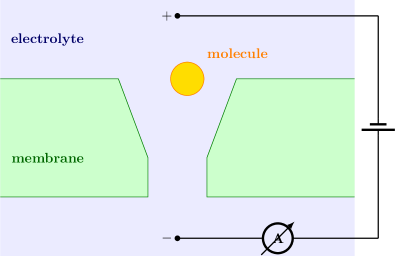
Figure 1: Schematic of a nanopore sensor. The pore connects two large electrolyte reservoirs (blue) separated by a membrane (green). A transmembrane voltage is applied (illustrated by two electrodes in a circuit diagram), triggering an ionic current through the pore. Target molecules (yellow) can be detected based on modulation of the current as they enter the nanopore.

Given the importance of the PNPS model in engineering, relatively few papers have addressed the numerical approach in detail. Splitting schemes for the time-dependent formulation have been analysed in [47, 51, 44]; but our interest lies in the steady-state distributions which can be obtained more efficiently directly, without time-stepping. Most works related to nanopore modeling rely on a black-box implementation provided by the commercial Comsol Multiphysics package [58, 57, 38, 35, 41]. In the microfluidic community, special-purpose finite difference codes have been shown to give better performance [29]. For our work, however, we prefer the flexibility of unstructured meshes to account for complex real-world nanopore geometries, which are defined, for instance, by the shapes of biological channel proteines like $\alpha$-hemolysin [54]. Therefore, finite elements will be used for discretization.

Our goal in this work was to create a state-of-the-art PNPS solver that overcomes the limitations of both off-the-shelf commercial solutions and highly structured geometries. The two main contributions to the numerical literature are

• a detailed investigation of linearization schemes for PNPS, and

• a fast adaptive mesh refinement scheme based on goal-oriented error estimation.

The adaptivity part is specifically tailored towards fast and reliable evaluation of the electrophoretic force on particles surrounded by the fluid, which we consider important for nanopore sensor modeling. The novelty compared to previous applications of goal-oriented adaptivity [4, 2], besides being the first for PNPS, is that we base the estimator not on the full PDE system but on a simplified model inspired by physics, namely, the linear Poisson-Boltzmann equation. Since solving the latter equation takes only a fraction of the time compared to the full system, this essentially renders the whole iterative mesh refinement procedure a cheap preprocessing step to be performed before the actual simulation. While by computing the estimator for a different equation we necessarily leave the realm of theoretical validity (where sometimes convergence of adaptive methods can be proved rigorously [19, 18, 7]), numerical results indicate that our approach does work surprisingly well (Section 4.3). The estimator not only qualitatively picks the correct regions for refinement, but also drives down the error in quantities of interest of the full model with the theoretically optimal rate $O(h^{2})$.

Our findings on linearization are of general interest for steady-state PNPS related models. To solve the PNPS equations – which form a nonlinear system of seven coupled equations –, we consider three linearization schemes: a monolithic Newton method applied to the whole system, a Gummel-type fixed-point method, and a hybrid scheme where Newton’s method is only applied to the PNP part. The fixed-point method uses a novel corrected Poisson equation which lowers iteration count significantly compared to similar approaches in the literature [39]. In our numerical comparisons, the fixed-point and hybrid methods both reveal some strengths and weaknesses, but clearly outperform the Newton method.

A third contribution of this work lies in modeling and is more specifically tied to the simulation of nanopore sensors. For sensor prototyping, solution of the PNPS system is just one building block to obtain the force which drives the transport of target molecules through the sensor. We investigate two different models for the force where the molecule is either finite-sized or point-sized. In the point-size model, the molecule has no influence on its surrounding electric field and fluid flow; this is a strong simplification, since the force on the whole domain can be obtained from a single PNPS solve. Indeed, we find that the two models deviate significantly from each other. However, we show how to calibrate the point-size model using a single evaluation of the finite-size model, to obtain a much better fit.

The remainder of the paper is organized as follows. The PNPS equations, including a description of boundary conditions and other modeling aspects are presented in Section 2. We also introduce a 2D version of the system in cylindrical coordinates that can simplify the simulation whenever the geometry is axisymmetric. Section 3 is devoted to numerical methods. Linearization of PNPS is discussed in 3.1, and further details of the numerical solver are given in Section 3.2. In Section 3.3 the goal-oriented adaptivity framework is introduced. We formulate an adaptive algorithm similar to [4, 49] which makes use of patch-wise extrapolation of the dual solution. Additionally, we propose a cheaper variant without extrapolation where the error estimator is based directly on the dual solution.

Numerical results are presented in Section 4. The geometry we use for experiments is modeled after the DNA-based nanopore sensor recently published in [5], where we carefully try to replicate the experimental set-up. In the Appendix, additional numerical results can be found which validate our solver against the exact solution on an idealized test problem. We conclude with Section 5.

2 Model

To start with a broad picture of what simulations of a nanopore sensor should achieve, consider the target molecule in Figure 1, and suppose the sensor is designed to detect exactly this molecule, which is of a certain shape and carries a certain charge. Two basic questions regarding the functionality of our sensor would be, first, whether the molecule can even enter the nanopore, and second, whether it would translocate the pore sufficiently slowly to be detected by measurements of ionic current. Both questions can for instance be addressed using the framework of the Langevin equation [34] for the dynamics of small particles.

In this or any similar framework, the specifics of the physical environment (i.e., sensor and molecule) enter through the electrophoretic force $\boldsymbol{F}(\boldsymbol{x})$ on the target molecule at any given position $\boldsymbol{x}$. Once the force is available in parametrized form, we can devise algorithms to compute quantities of interest such as mean translocation time and probability. The physical model underlying $\boldsymbol{F}(\boldsymbol{x})$ is encapsulated in the PNPS equations, which are the focus of our work and are discussed now.

2.1 PNPS equations

The steady-state Nernst-Planck (NP) equations for a 1:1 electrolyte with positive and negative ion concentrations $c^{+}$ and $c^{-}$, respectively, are given by

$$\nabla\cdot\boldsymbol{j}^{\pm} =0,$$ (1a)

$$\boldsymbol{j}^{\pm} =-D^{\pm}\nabla c^{\pm}\mp\frac{qD^{\pm}}{kT}c^{\pm}\nabla\phi+c^{\pm}\boldsymbol{u}.$$ (1b)

The quantity $\boldsymbol{j}^{\pm}$ is called the ionic flux; $D^{\pm}$ is the ion-specific diffusion coefficient; $q$ the elementary charge; $\phi$ the electric potential; and $\boldsymbol{u}$ the fluid velocity. This differs from the more well-known form of the Nernst-Planck equations [9] by the convective flux term $c^{\pm}\boldsymbol{u}$, which introduces coupling to the Stokes equation; the term describes transport of ions with the surrounding background medium, water. The ion concentrations $c^{\pm}$ are measured in molar units $\text{mol}/\text{m}^{3}$ and will therefore be multiplied by the Faraday constant $F=96485\text{ C}/\text{mol}$ to give rise to a charge concentration.

Notably, we will not assume that the diffusion coefficients $D^{\pm}$ are constant and equal to their bulk value. It has been recognized in the literature that the confining environment of a narrow channel can substantially reduce diffusivity [45, 46, 14, 10, 25, 32], so we have built this possibility into our solver. In the numerical experiments below, we use a bulk value of $D^{\pm}=1.9\text{ nm}^{2}/\text{ns}$ for both ions, which is lowered by a factor of $0.5$ inside nanopores. For absolute temperature we use $T=293$ K.

The Poisson equation for the electric potential $\phi$ is

$$-\nabla\cdot\left(\varepsilon\nabla\phi\right)=\rho_{0}+F(c^{+}-c^{-})$$ (2)

with $\varepsilon$ denoting the material-dependent electric permittivity and $\rho_{0}$ permanent charges present in the system, e.g. in target molecules and on the pore walls. Equivalently, permanent charges located on a surface are incorporated via Neumann boundary or interface conditions.

Finally, the fluid velocity field $\boldsymbol{u}$ and pressure $p$ are determined by the Stokes equations, which read, in conservative form,

$$-\nabla\cdot\left[\eta\left(\nabla\boldsymbol{u}+\nabla\boldsymbol{u}{}^{T}\right)-pI\right] = -F(c^{+}-c^{-})\nabla\phi,$$ (3a)

$$\nabla\cdot\boldsymbol{u} = 0.$$ (3b)

Here, $\eta=10^{-3}$ $\text{Pa}\cdot\text{s}$ is the viscosity and $I$ is the identity tensor. The right hand side is the force arising from ions which are pushed by the electric field, dragging along nearby water molecules. The nonlinear inertial term $\boldsymbol{u}\cdot\nabla\boldsymbol{u}$ usually present in the Navier-Stokes equations can be neglected, since the Reynolds number in nanopore-related systems is very low.

Taking together (1)–(3), the PNPS system consists of seven equations for the seven unknowns: the electric potential $\phi$, the two ion concentrations $c^{+}$ and $c^{-}$, the three components of the velocity $\boldsymbol{u}$ and the pressure $p$.

2.2 Geometry and boundary conditions

We solve PNPS on a space domain like that pictured in Figure 1 on page 1. It consists of an aqueous pore embedded in a solid membrane and possibly a solid sphere inside or near the pore which represents the target molecule. The membrane separates two cylindrical reservoirs of electrolyte which extend the computational domain to about $20$ nm in every direction; this has been empirically confirmed large enough to ensure that the physics inside the pore are not disturbed by artificial boundary conditions, by comparing with reservoir sizes of up to $1000$ nm.

The Stokes and Nernst-Planck equations for the velocity and ion concentrations are solved only in the fluid part of the domain; the Poisson equation, on the other hand, is solved on the whole domain including membrane and molecule. The pore/membrane may consist of several distinct dielectric materials depending on the exact sensor to be modeled. Details for a concrete application set-up are provided in Section 4.1.

Boundary conditions are specified as follows. For the ions, we fix concentrations on the top and bottom of the computational domain at a bulk value $c^{\pm}=c_{{\rm 0}}$ (Dirichlet condition), while on other boundaries we apply a no-flux (Neumann) condition, $n\cdot\boldsymbol{j}^{\pm}=0$, which models hard repulsion at the pore walls.

The external electric field is applied by setting the potential to $\phi=0$ on the top and to a suitable bias such as $\phi=-0.1$ V on the bottom. On the outer barrel of the cylindrical reservoirs, the Neumann condition $\partial_{n}\phi=0$ is applied, assuming that sufficiently far from the influence of the pore the potential varies only in the direction perpendicular to the membrane. Interface conditions are used to incorporate charges sitting on the pore walls, i.e. $[\varepsilon\partial_{n}\phi]=\rho$ where $[\,\cdot\,]$ denotes the jump across the interface and $\rho$ the surface charge density. Charges on the target molecule, on the other hand, are incorporated via a volume term $\rho_{0}$ on the right hand side of the Poisson equation (2); in this way, the electric force on the molecule can be evaluated consistently by integrating $-\rho_{0}\nabla\phi$ over the molecule.

For the fluid velocity, we use the no-slip condition $\boldsymbol{u}=0$ on fluid-solid interfaces and the natural stress-free boundary condition on the outer reservoir boundaries. In addition, we fix the pressure by setting it to zero on the reservoir top.

2.3 Axisymmetric reduction

Most nanopores can be modeled to a good approximation as symmetric around the central $z$ axis. In fact, all the 3D geometries we implemented can be generated by rotation of a two-dimensional cross-section about this axis. In such a setting, if the target molecule is either not present at all or sits on the central axis, all the equations will possess axial symmetry. By transforming to cylindrical coordinates $r,\ \varphi,\ z$ and using the fact that the solutions do not depend on the angular component $\varphi$, the PNPS equations become a system of PDEs in the two variables $r,\ z$. This 2D axisymmetric version is much faster to solve and was implemented in addition to the full 3D version to provide validation and rapid calculations for set-ups without off-centered molecules.

The idea of using axial symmetry to reduce computational effort is not new in the context of nanopores. In fact, [38, 35, 41, 42] – which are the publications most similar in scope to this one – all restrict themselves to axisymmetric settings, so the novelty of our implementation rather lies in the fact that we handle the full 3D case as well.

2.4 Physical Quantities of Interest

Since we want to describe translocation of target molecules through a nanopore, the primary output of our PNPS solver will be the mean force $\boldsymbol{F}$ acting on such a molecule, which we model as a sum of two contributions

$$\boldsymbol{F}=\boldsymbol{F}_{{\rm el}}+\boldsymbol{F}_{{\rm drag}}.$$ (4)

$\boldsymbol{F}_{{\rm el}}$ is the electric force induced by the electric field acting on charges on the molecule, and $\boldsymbol{F}_{{\rm drag}}$ is the drag force exerted on the molecule surface by the moving fluid.

Finite-sized molecule

For our main model, we build a spherical target molecule into the geometry by excluding its volume from the fluid domain and ensuring that the mesh aligns with the molecule boundaries. Then, the forces are given by

$$\boldsymbol{F}_{{\rm el}}=-\int_{M}\rho_{0}\nabla\phi$$ (5)

and

$$\boldsymbol{F}_{{\rm drag}}=\int_{\partial M}n\cdot\sigma$$ (6)

respectively, where $M$ is the part of the domain occupied by the molecule, $\rho_{0}$ the molecule surface charge density and $\sigma=\eta\left(\nabla\boldsymbol{u}+\nabla\boldsymbol{u}{}^{T}\right)-pI$ the fluid stress tensor.

Note that the drag force in formula (6) is expressed as a surface integral. In practice, we actually evaluate drag component-wise as the volume integral

$$F_{{\rm drag}}^{i}=\int_{\Omega_{F}}\sigma:\nabla\boldsymbol{z}_{i}-\boldsymbol{f}\cdot\boldsymbol{z}_{i}$$ (7)

where $\Omega_{F}$ is the fluid domain (excluding the molecule), $\boldsymbol{f}=-F(c^{+}-c^{-})\nabla\phi$ the volume force and $\boldsymbol{z}_{i}$ any vector field that satisfies $\boldsymbol{z}_{i}|_{\partial M}=\boldsymbol{e}_{i}$ where $\boldsymbol{e}_{i}$ is the $i$-th unit vector. This representation is equivalent to (6) if $\boldsymbol{u}$ and $p$ solve the Stokes equation exactly, as can be shown via integration by parts. Formula (7) was reported by others [4] and observed by ourselves to yield a more accurate numerical approximation. For $\boldsymbol{z}_{i}$ we use a piece-wise linear interpolation of $\boldsymbol{e}_{i}$ on the molecule boundary and zero elsewhere.

Point-sized molecule

If the PNPS equations are solved on a geometry without target molecule, we can still obtain an estimate for $\boldsymbol{F}_{{\rm el}}$ and $\boldsymbol{F}_{{\rm drag}}$ on every given position of the computational fluid domain. In this case, we neglect the influence that the charge and geometrical presence of the molecule has on the physical environment, and assume the molecule to be located at a single point. The electric force is then given by

$$\boldsymbol{F}_{{\rm el}}^{*}(x)=-Q\nabla\phi(x)$$ (8)

where $x$ is the molecule position and $Q$ the total charge on the molecule. The drag force is more difficult, since it would actually vanish for a point-sized molecule, but we still want a reasonable estimate for a spherical molecule of finite radius $r>0$. We approximate it by Stokes’ law

$$\boldsymbol{F}_{{\rm drag}}^{*}(x)=6\pi\eta r\boldsymbol{u}(x).$$ (9)

Because of confinement inside the pore, we anticipate that using equation (9) could lead to an underestimation of the drag force [46]. This is confirmed in Section 4.4, where the discrepancy between the two models $\boldsymbol{F}$ and $\boldsymbol{F}^{*}:=\boldsymbol{F}_{{\rm el}}^{*}+\boldsymbol{F}_{{\rm drag}}^{*}$ (finite-sized and point-sized molecule) is investigated. We shall also elaborate on possible improvements to the point-size model.

2.5 The Poisson-Boltzmann approximation

Close to equilibrium, ion concentrations are well approximated by the Boltzmann factors

$$c^{\pm}=c_{0}e^{\mp\frac{q}{kT}\phi}$$

where $c_{0}$ is the bulk concentration of both ion species. For zero voltage bias, this is the exact solution to the Nernst-Planck equations (1) without the convective flux term $c^{\pm}\boldsymbol{u}$ (in this case, $\boldsymbol{j}^{\pm}=0$ and the boundary condition $c^{\pm}=c_{0}$ is matched exactly if the potential is zero at the boundary). But even for low to moderate biases and with convective flux included, Boltzmann factors provide a useful estimate for the ion distributions near charged walls. By plugging the Boltzmann distribution into the Poisson equation (2), one obtains the Poisson-Boltzmann (PB) equation

$$-\nabla\cdot\left(\varepsilon\nabla\phi\right)+\chi_{F}2qc_{0}\sinh\frac{q\phi}{kT}=\rho_{0},$$

where $\chi_{F}$ denotes the characteristic function of the fluid domain. By using the linearization $\sinh(z)\approx z$, we arrive at the linear Poisson-Boltzmann equation

$$-\nabla\cdot\left(\varepsilon\nabla\phi\right)+\chi_{F}\frac{2q^{2}c_{0}}{kT}\phi=\rho_{0}.$$ (10)

This gives us a simplified model for the electric potential. In Section 3.3, we construct an error indicator solely based on solutions to the linear PB equation, which is orders of magnitude cheaper than solutions of the full PNPS model. Thus, we use equation (10) for mesh pre-refinement before the actual PNPS simulation. The linearity also makes it fit better into the framework of goal-oriented adaptivity.

In addition, the PB approximation can serve as initial guess for Newton iteration of the PNP equations. This helps with convergence issues caused by high surface charges, as shown in Section 4.2.

3 Numerical Method

We use a finite element discretization for all the equations of the PNPS system, which was implemented in Python on top of the open-source finite element package Fenics [36]. It allows us to easily handle unstructured meshes on irregular geometries and a wide variety of variational formulations and boundary conditions. The solver is released as a Python package, with all of our code made available online.

3.1 Linearization of PNPS

The PNPS system is nonlinear in the potential $\phi$, concentrations $c^{\pm}$ and velocity $\boldsymbol{u}$ and therefore has to be solved by some iterative linearization procedure. These procedures can be distinguished by whether they use Newton’s method, or fixed-point iteration, or a combination. Along these lines we will describe three different methods for the PNPS system. They will be compared numerically in Section 4.2.

Newton method

The first, black box approach to linearization is to apply Newton’s method to the whole system. Let us write our nonlinear equation in abstract variational form,

$$F(U)=0,$$

where $U=(\phi,c^{+},c^{-},\boldsymbol{u},p)$ represents the finite element solution and $F(U)$ is a linear functional on the discrete test space. Then, Newton’s method consists in successive linear solves of

$$DF(U)\delta U=-F(U),$$ (11)

followed by updates $U=U+\delta U$. As initial value, for instance, $U=(\phi,c^{+},c^{-},\boldsymbol{u},p)=(0,c_{0},c_{0},0,0)$ can be used. Written out, equation (11) amounts to solving the system

$$-\nabla\cdot(\varepsilon\nabla\delta\phi)-F(\delta c^{+}-\delta c^{-}) = \rho_{0}+\nabla\cdot(\varepsilon\nabla\phi)+F(c^{+}-c^{-}),$$ (12a)

$$\nabla\cdot\left[-D^{+}\nabla\delta c^{+}-\mu^{+}\delta c^{+}\nabla\phi+\delta c^{+}\boldsymbol{u}-\mu^{+}c^{+}\nabla\delta\phi+c^{+}\delta\boldsymbol{u}\right] = \nabla\cdot\left[D^{+}\nabla c^{+}+\mu^{+}c^{+}\nabla\phi-c^{+}\boldsymbol{u}\right],$$ (12b)

$$\nabla\cdot\left[-D^{-}\nabla\delta c^{-}+\mu^{-}\delta c^{-}\nabla\phi+\delta c^{-}\boldsymbol{u}+\mu^{-}c^{-}\nabla\delta\phi+c^{-}\delta\boldsymbol{u}\right] = \nabla\cdot\left[D^{-}\nabla c^{-}-\mu^{-}c^{-}\nabla\phi-c^{-}\boldsymbol{u}\right],$$ (12c)

$$-\eta\Delta\delta\boldsymbol{u}+\nabla\delta p+F(\delta c^{+}-\delta c^{-})\nabla\phi+F(c^{+}-c^{-})\nabla\delta\phi = \eta\Delta\boldsymbol{u}-\nabla p-F(c^{+}-c^{-})\nabla\phi,$$ (12d)

$$\nabla\cdot\delta\boldsymbol{u} = -\nabla\cdot\boldsymbol{u},$$ (12e)

which is a linearized version of PNPS in the unknowns $\delta U=(\delta\phi,\delta c^{+},\delta c^{-},\delta\boldsymbol{u},\delta p)$. Here we use $\mu^{\pm}:=\frac{qD^{\pm}}{kT}$ for readability. We will refer to this algorithm as the (full) Newton method:

Initialize $U=(\phi,c^{+},c^{-},\boldsymbol{u},p)$. Then:

1. Solve (12) for the Newton update $\delta U=(\delta\phi,\delta c^{+},\delta c^{-},\delta\boldsymbol{u},\delta p)$.

2. Update $U=U+\delta U$.

3. Let the relative error be defined by

   $$\text{error}:=\frac{\mathbb{\|}\delta U\|_{L^{2}(\Omega)}}{\mathbb{\|}U\|_{L^{2}(\Omega)}}.$$

   Check convergence (with tolerance $\tau>0$):

   1. If $\text{error}<\tau$, stop.

   2. Else, go back to 1.

Algorithm 1 Newton method for PNPS

Hybrid method

The full Newton method yields a single large system for linear solving. We suspected that computational effort could be saved by separating the equations into two smaller subsets, namely the PNP and Stokes systems, and solving them in an alternating fashion until convergence is reached, i.e., by a fixed-point iteration. Thus, the potential $\phi$ and concentrations $c^{\pm}$ will be obtained from the PNP part of the system, with the initial velocity set to zero. Then, Stokes will be solved for the velocity $\boldsymbol{u}$ and pressure $p$, with $\phi$, $c^{+}$, $c^{-}$ as input; the velocity will now be plugged into PNP, etc.

In this formulation, the Stokes part of the system is linear, but we still need to address the remaining nonlinearity in the PNP part (namely, the products $c^{\pm}\nabla\phi$). We could again simply apply Newton’s method to the PNP system only, or use an inner fixed-point loop. Both methods are well-established in the context of the PNP equations without velocity term [39, 37]; however, the fixed-point method is usually reported to require some form of under-relaxation, resulting in several hundreds of iterations until convergence [39].

In practice, we initially experimented with a naive, unrelaxed fixed-point iteration for PNP but found it to diverge in every case considered. Newton iteration, applied to the PNP part only, was seen to be quite robust, even with the constant initial guess $\phi=0$, $c^{\pm}=c_{0}$; in situations where it does not converge either, resources such as a better initial guess and under-relaxation (damped Newton) can still be used. Regarding the fixed-point iteration between PNP and Stokes, convergence was always observed; the coupling between these two systems, which stems from the convective flux term $c^{\pm}\boldsymbol{u}$ in the Nernst-Planck equation (1), seems to be sufficiently weak.

Taking this into consideration, the second method we propose consists of an outer fixed-point loop decoupling the system into a PNP and a Stokes part, and an inner Newton iteration to solve the PNP part. As a further refinement, it was found beneficial not to solve the PNP equations to full convergence in every step, but only to perform a single Newton iteration for every linear Stokes solve. We call this version of the algorithm the hybrid method:

Initialize $U_{\text{PNP}}=(\phi,c^{+},c^{-})$ and $U_{\text{Stokes}}=(\boldsymbol{u},p)$. The Newton update equation for the PNP system is

$$-\nabla\cdot(\varepsilon\nabla\delta\phi)-F(\delta c^{+}-\delta c^{-}) = \rho_{0}+\nabla\cdot(\varepsilon\nabla\phi)+F(c^{+}-c^{-}),$$ (13a)

$$\nabla\cdot\left[-D^{+}\nabla\delta c^{+}-\mu^{+}\delta c^{+}\nabla\phi+\delta c^{+}\boldsymbol{u}-\mu^{+}c^{+}\nabla\delta\phi\right] = \nabla\cdot\left[D^{+}\nabla c^{+}+\mu^{+}c^{+}\nabla\phi-c^{+}\boldsymbol{u}\right],$$ (13b)

$$\nabla\cdot\left[-D^{-}\nabla\delta c^{-}+\mu^{-}\delta c^{-}\nabla\phi+\delta c^{-}\boldsymbol{u}+\mu^{-}c^{-}\nabla\delta\phi\right] = \nabla\cdot\left[D^{-}\nabla c^{-}-\mu^{-}c^{-}\nabla\phi-c^{-}\boldsymbol{u}\right].$$ (13c)

Now,

1. Solve (13) for the Newton update $\delta U_{\text{PNP}}=(\delta\phi,\delta c^{+},\delta c^{-})$.

2. Update $U_{\text{PNP}}=U_{\text{PNP}}+\delta U_{\text{PNP}}$.

3. Save $U_{\text{Stokes},0}=U_{\text{Stokes}}$ from the last iteration.
   Solve the Stokes equation (3) for $U_{\text{Stokes}}$.

4. Set $\delta U_{\text{Stokes}}=U_{\text{Stokes}}-U_{\text{Stokes},0}$. Let the relative error be defined by

   $$\text{error}:=\frac{1}{2}\left(\frac{\mathbb{\|}\delta U_{\text{PNP}}\|_{L^{2}(\Omega)}}{\mathbb{\|}U_{\text{PNP}}\|_{L^{2}(\Omega)}}+\frac{\mathbb{\|}\delta U_{\text{Stokes}}\|_{L^{2}(\Omega)}}{\mathbb{\|}U_{\text{Stokes}}\|_{L^{2}(\Omega)}}\right).$$

   Check convergence (with tolerance $\tau>0$):

   1. If $\text{error}<\tau$, stop.

   2. Else, go back to 1.

Algorithm 2 Hybrid method for PNPS

Fixed-point method

Regardless of initial failure, we still wanted to see if a fast fixed-point solution was possible. We took inspiration from a practice common in the semiconductor community, which is to introduce the so-called Slotboom variables [53]

$$\tilde{c}^{\pm}=c^{\pm}e^{\pm\frac{q}{kT}\phi}.$$

For motivation, note that in equilibrium – when the Boltzmann distribution applies – $\tilde{c}^{\pm}$ reduce to constants. Plugging these new variables into the classical Nernst-Planck equations (without velocity) renders them in purely self-adjoint form, which is usually emphasized [39]. But, more importantly for us, it also alters the form of the Poisson equation:

$$-\nabla\cdot\left(\varepsilon\nabla\phi\right)=F(\tilde{c}^{+}e^{-\frac{q}{kT}\phi}-\tilde{c}^{-}e^{\frac{q}{kT}\phi}).$$

Note that the potential $\phi$ now appears also on the right hand side, in the charge distribution term. The Poisson equation becomes nonlinear in the potential. If this would be solved in a fixed-point loop, where $\tilde{c}^{\pm}$ are taken from the last iteration, the new potential would not only give rise to a new charge distribution, but would already reflect part of the impact this change has on itself. This is just the correction that is needed to prevent the fixed-point iteration from exploding. In semiconductor device modeling, this type of iteration is known as Gummel’s method [24, 30].

With this new insight, we can actually change back to the old variables $c^{\pm}$, by using $\tilde{c}^{\pm}=c^{\pm}e^{\pm\frac{q}{kT}\phi_{0}}$ with $\phi_{0}$ being the potential from the last iteration, to find

$$-\nabla\cdot\left(\varepsilon\nabla\phi\right)=F(c^{+}e^{-\frac{q}{kT}(\phi-\phi_{0})}-c^{-}e^{\frac{q}{kT}(\phi-\phi_{0})}).$$

In the limit of convergence of the fixed-point iteration we have $\phi=\phi_{0}$ and the exponential terms vanish. Since those are artificial correction terms anyway, we might as well make our life easier and linearize them as

$$e^{\pm\frac{q}{kT}(\phi-\phi_{0})}\approx 1\pm\frac{q}{kT}(\phi-\phi_{0}).$$

Reordering, we arrive at a corrected Poisson equation which is again linear in the unknown $\phi$ and features the previous potential $\phi_{0}$ on the right hand side:

$$-\nabla\cdot\left(\varepsilon\nabla\phi\right)+\frac{Fq}{kT}\phi(c^{+}+c^{-})=F(c^{+}-c^{-})+\frac{Fq}{kT}\phi_{0}(c^{+}+c^{-}).$$ (14)

Alternating the corrected Poisson equation (14) with the unmodified Nernst-Planck and Stokes equations yields our proposed fixed-point method, summarized in Algorithm 3. To ensure convergence of the method, we recommend to start with two pure PNP iterations and only afterwards include the Stokes equation in the iteration.

Initialize $\phi$, $c^{+}$, $c^{-}$ and $U_{\text{Stokes}}=(\boldsymbol{u},p)$. Set the iteration count to $i=0$. Then:

1. Save the solutions from the previous iteration: $\phi_{0}=\phi$, $c_{0}^{+}=c^{+}$, etc.

2. Solve the corrected Poisson equation (14) for $\phi$.

3. Solve both the Nernst-Planck equations (1) for $c^{+}$, $c^{-}$.

4. If $i<2$, set $i=i+1$ and go back to 1.

5. Solve the Stokes equation (3) for $U_{\text{Stokes}}$.

6. Define the updates $\delta\phi=\phi-\phi_{0}$, etc. Let the relative error be defined by

   $$\text{error}:=\frac{1}{4}\left(\frac{\mathbb{\|}\delta\phi\|_{L^{2}(\Omega)}}{\mathbb{\|}\phi\|_{L^{2}(\Omega)}}+\frac{\mathbb{\|}\delta c^{+}\|_{L^{2}(\Omega)}}{\mathbb{\|}c^{+}\|_{L^{2}(\Omega)}}+\frac{\mathbb{\|}\delta c^{-}\|_{L^{2}(\Omega)}}{\mathbb{\|}c^{-}\|_{L^{2}(\Omega)}}+\frac{\mathbb{\|}\delta U_{\text{Stokes}}\|_{L^{2}(\Omega)}}{\mathbb{\|}U_{\text{Stokes}}\|_{L^{2}(\Omega)}}\right).$$

   Check convergence (with tolerance $\tau>0$):

   1. If $\text{error}<\tau$, stop.

   2. Else, go back to 1.

Algorithm 3 Fixed-point method for PNPS

3.2 Details of the numerical solver

Variational formulations for the PNPS related systems were obtained by integration by parts of equations (1)–(3), (10), (12)–(14) respecting their conservative structure; this was done for both the full 3D and 2D axisymmetric cases. The formulation of the Stokes system in cylindrical coordinates can be found in [12]. Dirichlet boundary conditions are enforced strongly, while Neumann conditions are incorporated naturally via boundary terms on the right hand side. For subequations of the PNP system, a standard $P^{1}$ finite element discretization is employed, while for the Stokes system, the consistent stabilized $P^{1}-P^{1}$ formulation by Hughes and Franca [27] is used to ensure inf-sup stability; for some of the numerical experiments below, we had to switch to a (more expensive) Taylor-Hood $P^{2}-P^{1}$ formulation for Stokes to enforce higher numerical accuracy.

In the 2D case, we always use a direct algebraic solver based on LU decomposition. This quickly turned out to introduce a memory and speed bottleneck in the 3D case, so we started experimenting with iterative solvers based on Krylov subspace methods for both the PNP and Stokes subsystems. The following choices are used subsequently for the 3D solver with the hybrid method: The PNP system (13) and PB equation (10), which are elliptic, are solved with BiCGstab [55] preconditioned by an incomplete LU factorization, and the Stokes system with the transpose-free quasi-minimal residual (TFQMR) method [20] preconditioned by the block preconditioner by Mardal and Winther [43]. For both solvers, the Fenics interface to PETSc [1] was employed, with the ILU implementation taken from the Hypre package [17].

For the PNP system, the iterative approach drastically improves computational speed in 3D even for moderately large meshes. For the Stokes system however, a large number (hundreds to thousands) of iterations are needed which renders the iterative approach quite slow, but at least the memory barrier is removed. Further research will have to shed light on constructing the right preconditioner for the Stokes system in a nanopore context, and explain why an established method [43] seems to fail here.

Meshes were generated with Gmsh [22] and the Python-Gmsh interface written by Schlömer. Curved boundaries, as present in all our pore geometries, were approximated by polygons. For mesh refinement, we modified the implementation in Fenics so that refined meshes respect the curved geometry.

3.3 Goal-oriented adaptivity

Solutions to the PNPS system generally exhibit multiscale features such as thin boundary layers near a charged surface. Overall simulation accuracy depends on whether these layers are resolved by a sufficiently fine mesh. However, since the main output of the simulation are scalar quantities of interest like the force on a target molecule (Section 2.4), the mesh has to be fine only in the locations that directly influence this quantity. Especially in 3D, the simulation time can quickly explode and get untractable if mesh refinement is applied too broadly.

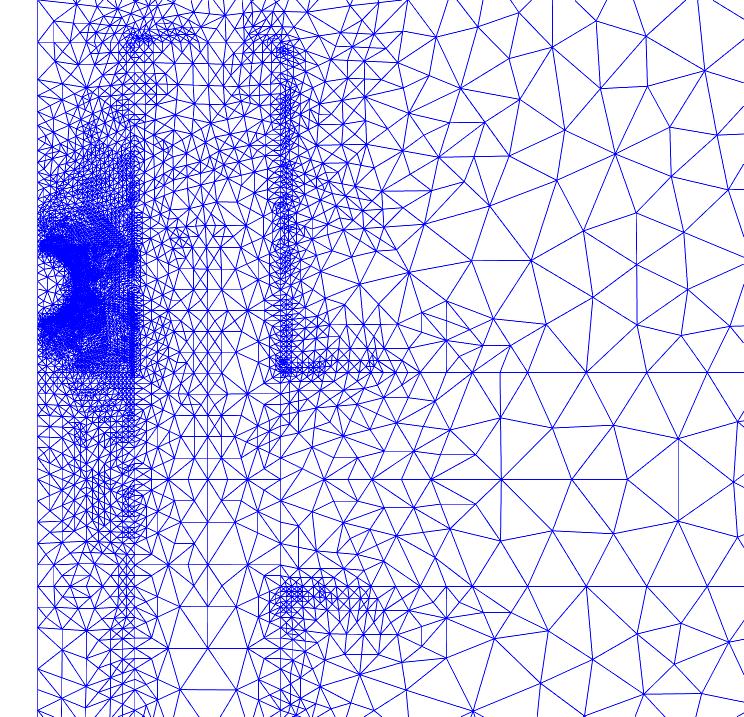
Figure 2: Refined mesh produced by the goal-oriented adaptive algorithm.

Figure 2 shows an example mesh on an axisymmetric pore geometry that fulfills these objectives: strong refinement at the boundary layers with emphasis on the positions around the molecule, but a coarse mesh outside the pore and far from the molecule. Clearly, such an approach to mesh refinement would be cumbersome to implement by hand and difficult to generalize. The method which accomplishes this automatically is adaptive refinement based on goal-oriented error estimation [4, 2], and will be described in this section.

General framework

To present the general ideas of goal-oriented adaptivity, suppose we want to solve a linear PDE in variational form

$$a(u,v)=L(v).$$ (15)

Goal-oriented means that we are interested in a quantity $F(u)\in\mathbb{R}$, where $F$ is a functional on the solution space and assumed to be linear. The Galerkin discretization of (15) yields a solution $u_{h}$ in a discrete subspace, and we want to refine the mesh such that the error in the goal functional compared to the true solution is small, i.e. decrease $|F(u-u_{h})|$. To analyze this error we introduce the dual solution $w$ which solves

$$a(v,w)=F(v).$$ (16)

Note that the arguments in the bilinear form have been swapped and the right hand side is now the goal functional. Equations (15) and (16) can be combined to give an error representation:

$$F(u-u_{h})=a(u-u_{h},w)=L(w)-a(u_{h},w)=:R(w).$$

The right-hand side is simply the residual of the Galerkin problem, evaluated at the dual solution $w$, and can in principle be computed once we have an approximation $w_{h}$ of $w$. Care must be taken at this point, however, because choosing $w_{h}$ from the same discrete space as $u_{h}$ yields $R(w_{h})=0$ due to Galerkin orthogonality, which is hardly a useful error estimate. One possible solution is to extrapolate $w_{h}$ patchwise to a higher-order function space [49, 2]. In the case when $w_{h}$ and $u_{h}$ are $P^{1}$ and the extrapolation $Ew_{h}$ is $P^{2}$, for example, one can expect that [2]

$$F(u-u_{h})=R(w)=O(h^{2})\quad\text{while}\quad R(Ew_{h})=R(w)+O(h^{3}).$$

This shows that $F(u-u_{h})\approx R(Ew_{h})$ produces an accurate estimate of the true error. A local error indicator is obtained by expanding the residual into a sum of local contributions,

$$R(w)=\sum_{T}R_{T}(w)+R_{\partial T}(w).$$

The local terms can be found by integration by parts on every mesh element $T$. Their absolute values

$$\eta_{T}:=\left|R_{T}(\tilde{w})+R_{\partial T}(\tilde{w})\right|$$ (17)

are the element-wise error indicators. Here we will use $\tilde{w}=Ew_{h}-w_{h}$ to make the residuals as small and the upper bound $|F(u-u_{h})|\leq\sum\eta_{T}$ as tight as possible. The error indicators $\eta_{T}$ (17) are used to decide which mesh elements will be refined, as outlined in the following classical adaptive algorithm.

Starting with an initial coarse mesh, do:

1. Solve the primal (15) and dual (16) problems for $u_{h}$, $w_{h}$.

2. Extrapolate $w_{h}$ to a higher-order approximation $Ew_{h}$.

3. Compute the error indicators (17).

4. Produce a refined mesh by bisecting the elements with the highest indicators.

5. Based on some criterion, either stop or go back to 1.

Algorithm 4 Adaptive algorithm

The patchwise extrapolation in step 2 is done using the Fenics implementation detailed by Rognes and Logg [49]. The number of elements to be refined in step 4 is determined by Dörfler marking [13]. As for the termination criterion in step 5, we will usually stop after a critical amount of elements is reached corresponding to a maximal work load.

Faster error estimation without extrapolation

In our implementation of the adaptive Algorithm 4, the most computationally expensive step is extrapolation of the dual solution to a higher-order function space. We expect this observation to hold independently of the precise extrapolation method, due to the blow-up of degrees of freedom when switching from a $P^{1}$ to a $P^{2}$ representation. As discussed, the extrapolation is done to avoid Galerkin orthogonality, improving the useless global estimate $F(u-u_{h})\approx R(w_{h})=0$ to an estimate of (sometimes provable) high accuracy $F(u-u_{h})\approx R(Ew_{h})$. However, that this also leads to local error indicators of high quality remains largely a heuristic, according to current wisdom about adaptive methods Feischl et al. [19].

In any case, we will apply error estimation only in an approximate way to a simplified model (explained below). One consequence is that the global error estimate we would get from the adaptive algorithm has no relevance to our actual quantities of interest. Once we dispense with a global error estimate and only want to compute local indicators, there is no longer a clear theoretical motivation to use the extrapolated dual solution $Ew_{h}$ rather than $w_{h}$. Consequently, we propose to exchange the indicators (17) for

$$\eta_{T}^{{\rm cheap}}:=\left|R_{T}(w_{h})+R_{\partial T}(w_{h})\right|.$$ (18)

Thus, we simply skip the extrapolation step and calculate our error indicators directly from the dual Galerkin solution. This leads to the following alternative adaptive Algorithm 5, which is both faster and simpler to implement than Algorithm 4.

Starting with an initial coarse mesh, do:

1. Solve the primal (15) and dual (16) problems for $u_{h}$, $w_{h}$.

2. Compute the cheap error indicators (18).

3. Produce a refined mesh by bisecting the elements with the highest indicators.

4. Based on some criterion, either stop or go back to 1.

Algorithm 5 Cheap adaptive algorithm without extrapolation

Interestingly, we are not aware of any publication that makes use of this simple idea, although it has also been proposed in the unpublished work [28]. The performance with respect to quantities of interest for our particular problem remains to be examined in Section 4.3.

Adaptivity for the Poisson-Boltzmann equation

Because two systems of equations have to be solved in every iteration of Algorithms 4 and 5, running it for the full PNPS model would be costly. Besides, as a nonlinear system it does not fit neatly into the framework sketched above (but see [2] for goal-oriented adaptivity in the nonlinear case). However, we expect a good deal of the error information to be already contained in a simplified physical model, namely, the linear PB equation. In our simulations, we will therefore proceed as follows:

1. Refine the mesh several times by goal-oriented adaptivity for the linear PB equation (10).

2. Solve the PNPS equations (1)–(3) once on the final mesh.

When we apply the general adaptivity framework to the linear PB equation, the bilinear form becomes

$$a(\phi,\psi)=\int_{\Omega}\varepsilon\nabla\phi\cdot\nabla\psi+\int_{\Omega}\kappa\phi\psi$$

with $\kappa:=\chi_{F}\frac{2q^{2}c_{0}}{k_{B}T}$ and $\chi_{F}$ the characteristic function of the fluid domain. The right hand side stems from a composition of volume and surface charges

$$L(\psi)=\int_{\Omega}\rho_{0}\psi+\int_{\Gamma}\rho\psi$$

with $\Gamma$ denoting all charged interfaces, e.g., pore walls. Both trial and test functions are restricted to vanish on the Dirichlet part of $\partial\Omega$. That is, even if the full PNPS model is specified with non-zero voltage bias, we always solve the auxiliary PB equation with zero voltage bias, since applying a non-zero bias would violate the assumptions underlying the PB model, leading to an unphysical, exponential behaviour of the potential at the Dirichlet boundary and an overestimation of error near this boundary.

The important remaining question is how to choose the goal functional. Ideally, our quantity of interest would be the force $\boldsymbol{F}$ on the target molecule (4), but computing it requires the full PNPS solution. Still, we may find a functional of the linear PB potential that roughly preserves the properties of the PNPS force, such as higher relevance of the region near the molecule. We aim to achieve this by defining

$$F(\phi):=-\int_{M}\rho_{0}\partial_{z}\phi$$ (19)

as our goal functional; $M$ is the molecule region and $\rho_{0}$ its charge density. This is a direct analogue of the electrical force (5) from the PNPS model; the electric field $-\nabla\phi$ is restricted to the $z$-direction because we need a scalar-valued functional. The hydrodynamic contribution to the force is neglected for lack of a reasonable analogue in the PB model.

It has to be emphasized that (19) shall not provide a quantitative estimate of the actual force $\boldsymbol{F}$ or its electrical part $\boldsymbol{F}_{\text{el}}$. The only purpose of the goal functional is to guide the adaptive mesh refinement process, and we must hope that the parts of the domain where the discretization error $F(\phi-\phi_{h})$ is high are the same parts where also the error in the actual quantity of interest $\boldsymbol{F}$ would be high. That this is indeed the case is verified experimentally in Section 4.3.

With these specializations of the general goal-adaptive framework, let $w$ denote the dual solution as before. The local error contributions can be obtained from the residual $R(w)$ via element-wise integration by parts by calculating

$$R(w)=-a(\phi_{h},w)+L(w)= \sum_{T}-\int_{T}\left(\varepsilon\nabla\phi\cdot\nabla w+\kappa\phi w\right)+\int_{T}\rho_{0}w+\frac{1}{2}\int_{\partial T}\rho w$$

$$= \sum_{T}\int_{T}\left(\varepsilon\nabla^{2}\phi-\kappa\phi+\rho_{0}\right)w+\frac{1}{2}\int_{\partial T}\left(\rho-[\varepsilon\partial_{n}\phi]\right)w$$

$$=: \sum_{T}(r_{T},w)_{T}+(r_{\partial T},w)_{\partial T}.$$

The strong cell and facet residuals are given by

$$r_{T} = \varepsilon\nabla^{2}\phi-\kappa\phi+\rho_{0},$$

$$r_{\partial T} = \frac{1}{2}\left(\rho-[\varepsilon\partial_{n}\phi]\right),$$

where $[\varepsilon\partial_{n}\phi]$ denotes the jump over a facet in normal direction. Here, $\rho$ is understood to be zero on uncharged facets, and on boundary facets $[\varepsilon\partial_{n}\phi]=\varepsilon\partial_{n}\phi$. The error indicators $\eta_{T}$, defined abstractly in (17) and (18), can now be explicitly written as

$$\eta_{T}=\left|(r_{T},\tilde{w})_{T}+(r_{\partial T},\tilde{w})_{\partial T}\right|$$

with either $\tilde{w}=(Ew_{h}-w_{h})$ or $\tilde{w}=w_{h}$. Goal-oriented adaptivity is implemented according to Algorithms 4 and 5. Once the adaptive loop has produced a mesh sufficiently resolving the regions of interest, the final Poisson-Boltzmann solution is used as an initial guess for the iteration solving the nonlinear PNPS equations.

4 Results and Discussion

In this section, we want to assess our numerical approach in detail and gain further insights into the modeling and simulation. To embed numerical experiments in a real-world application setting, we introduce a 3D model of the nanopore sensor recently published in [5].

For a basic validation of the correctness of our implementation, we also carried out experiments on an idealized test problem where a semi-analytical solution is possible. They can be found in the Appendix A.1.

4.1 DNA-based nanopore sensor

We describe the DNA-based nanopore sensor model inspired by [5]. The pore consists of six vertically aligned $9$ nm short DNA strands arranged in a circle, forming a hole of width approximately $5$ nm. As shown in Fig. 3, we modeled the DNA pore wall and hole by two concentric cylinders of radii $2.5$ and $1\text{ nm}$, respectively (thus assuming the DNA thickness to be $1.5$ nm on average). The pore resides in a lipid bilayer membrane of thickness $2.2$ nm, and the whole system is placed in the center of a cylindrical electrolyte reservoir of height $20$ nm and radius $10$ nm. We use relative electrical permittivities $\varepsilon_{r}=80.2$ for water, $\varepsilon_{r}=2$ for the lipid bilayer and $\varepsilon_{r}=12$ for DNA. In some of the following numerical experiments, we also include a spherical target molecule, as depicted in Fig. 3, which has $\varepsilon_{r}=12$. Without an off-centered molecule, the domain is axisymmetric and simulations can optionally be done with the 2D solver.

Concerning boundary conditions, the DNA surface (inner and outer pore wall, except the outer part which touches the membrane) is equipped with a uniform negative surface charge density $\rho_{\text{DNA}}$, while the membrane was assumed uncharged; a potential bias $\Delta V$ is applied on the bottom of the domain; and both ion concentrations are fixed to a bulk value $c_{0}$ on the top and bottom. If not stated otherwise, the numerical values used are $\rho_{\text{DNA}}=-0.25$$q/\text{nm}^{2}$, $\Delta V=-100$ mV and $c_{0}=300$ $\text{mol}/\text{m}^{3}$. The molecule is equipped with a fixed total charge of $-q$, which is spread uniformly across the volume occupied by the discretized molecule.

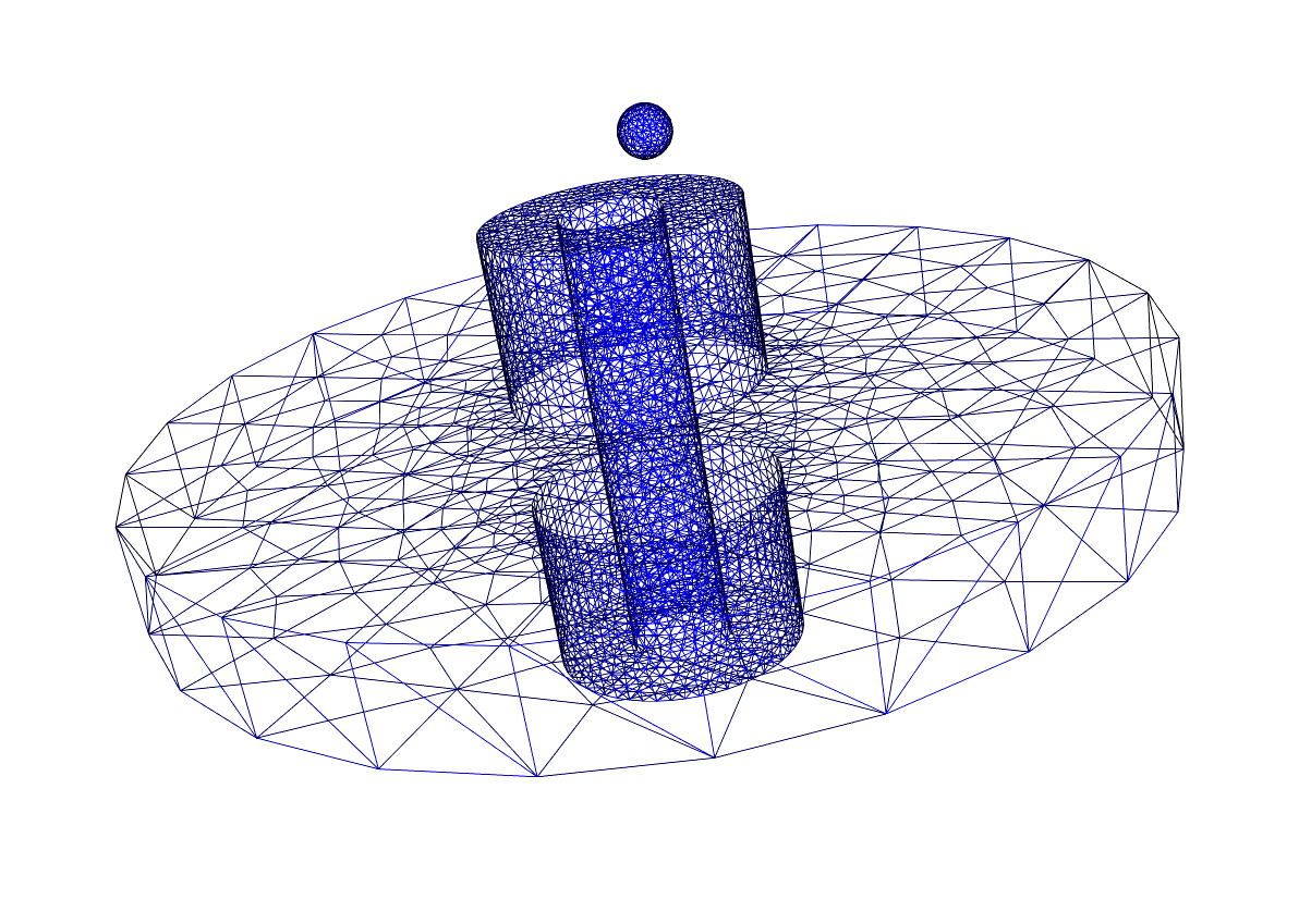
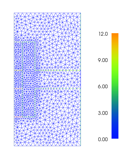
Figure 3: DNA nanopore model. Shown are the 3D mesh of the pore, membrane and molecule, and the 2D mesh of a half-plane on which the problem is solved in the axisymmetric formulation. The geometry is inspired by [5].

4.2 Comparison of linearization schemes

In Section 3.1, we proposed three approaches for linearization of the PNPS system, which we now compare regarding convergence speed and robustness. We consider the axisymmetric (2D) formulation without target molecule as pictured in Fig. 3 (right), with a fixed quasi-uniform mesh size with $h\approx 0.1$ nm.

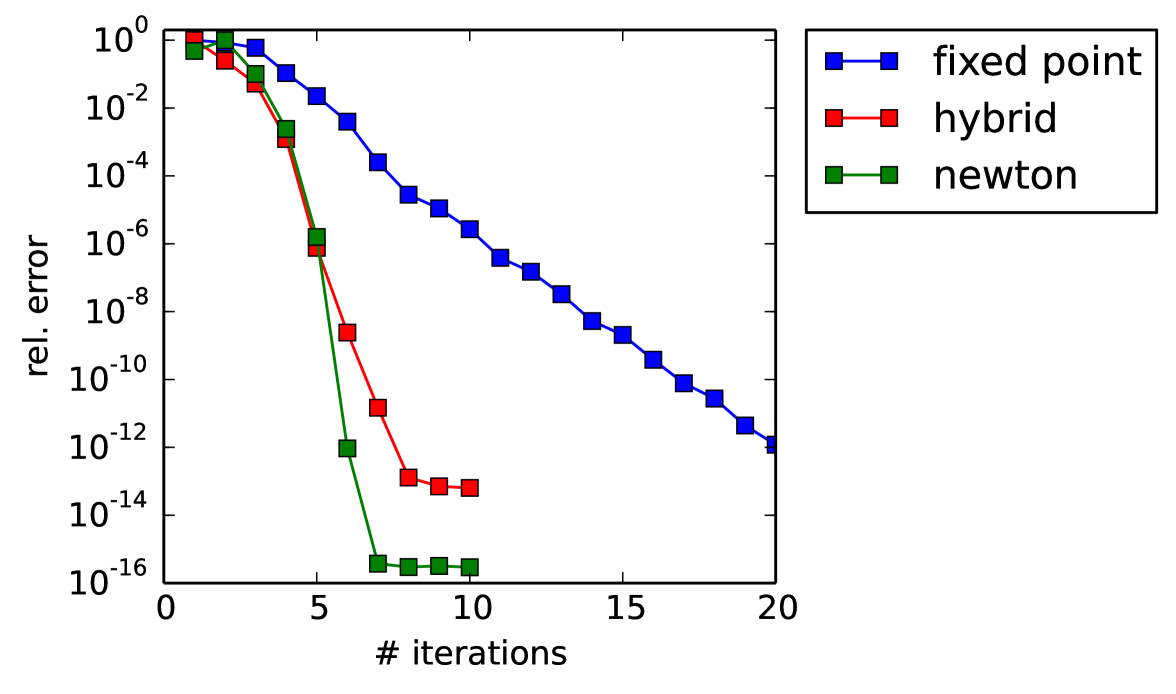
(a) Linearization error vs. iteration count

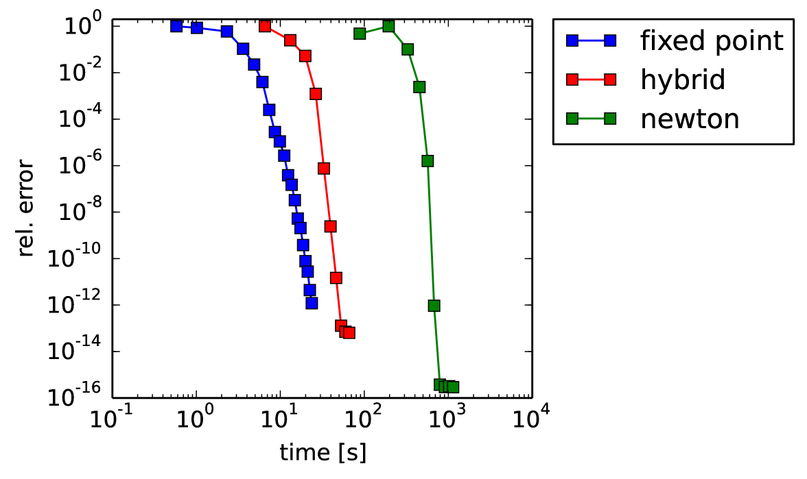
(b) Linearization error vs. CPU time

Figure 4: Comparison of the linearization error between the Newton, hybrid and fixed-point methods. The error is computed as defined in Algorithms 1, 2 and 3, respectively.

Comparison of convergence speed

Figure 4(a) compares convergence speed of the Newton, hybrid and fixed-point methods in terms of the number of iterations. The voltage bias was lowered to $-50$ mV in this example to ensure convergence of all three schemes. The two Newton-based methods exhibit fast, superlinear convergence at first; the hybrid method deviates from this only in the last few steps and settles for the expected linear asymptotic rate. For the fixed-point method, a slower linear convergence rate can be observed. This indicates that the nonlinearity in the PNP system is far stronger than the coupling between PNP and Stokes, and the iteration between the latter two converges very fast.

In terms of computational time, the picture is turned upside down, because a single iteration of the fixed point scheme is much faster than for the other schemes. All in all, as shown in Figure 4(b), the fixed point method clearly wins in terms of convergence speed. If we compare the times when an accuracy of $4$ digits is first reached, fixed-point (with $8.6$ seconds) is $3.8\times$ faster than hybrid ($33$ seconds) and $67\times$ faster than Newton (over $9$ minutes) in this particular example. On smaller meshes than shown in the figure, all three methods are closer, meaning the segregated approaches scale better with mesh size.

To put these results into the right perspective, let us note that in Figure 4(b), computational times are dominated by the algebraic linear solver, and that we used a direct method for solving – which has $O(N^{3/2})$ complexity in the number of variables [21] and thus gives an inherent advantage to decoupled systems, as $2(N/2)^{3/2}<N^{3/2}$. This could be considered an unfair comparison and raises the question whether the advantage remains if an iterative solver of optimal complexity $O(N)$ is used. However, choosing a good preconditioner for the full Newton system seems a more difficult task than for the segregated solvers. For the hybrid and fixed-point methods, the PNP and Stokes subsystems can be treated separately, which makes them more convenient when an iterative solver is used.

In the case that an LU solver is used, like here, there is an additional tweak for the fixed-point and hybrid method that we have not mentioned: Since the bilinear form of the Stokes equations is not changing, the system matrix has to be assembled and factorized only once. This makes the dominance of the fixed point method even more pronounced, but for comparison’s sake it was not used in Figure 4(b).

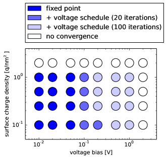
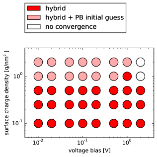
Figure 5: Robustness of convergence of hybrid and fixed-point schemes with respect to voltage bias/surface charge. The colored circles represent values of voltage and surface charge where the respective iteration converges. Convergence is defined as the linearization error (see Figure 4) falling below $\text{tol}=10^{-3}$; in case of non-convergence the solution either exploded or, for of the fixed-point methods with voltage schedule, an allowed number of iterations was exceeded. Lighter colors are meant to subsume darker colors; i.e. the hybrid method + PB initial guess converges for same values as the hybrid method (red) plus additional values which are colored in light red. A white circle indicates that none of the respective methods converged.

Comparison of convergence robustness

Next, we compare robustness of convergence with respect to variations of the model parameters. In the speed comparison, parameters where chosen deliberately so that all three linearization methods converged. But, as we will show, either of the methods diverges if some input parameters are made large enough. We want to explore and be aware of these convergence boundaries, as far as they are relevant to realistic models.

The two parameters we identified as critical for convergence are surface charge and voltage bias. Interestingly, the hybrid method is mainly sensitive to surface charge but not to voltage bias, while for the fixed-point method the opposite is true. In Figure 5, we illustrate the region of convergence for these two methods in the 2D plane of DNA surface charge and voltage bias parameters, with the (negative) surface charge density ranging up to $2q/\text{nm}^{2}$ and the (negative) voltage up to $2$ V. We disregard the full Newton method at this point because of its unfavourable speed performance, and because we observed its robustness properties to be similar to the hybrid method.

The parameter values for which convergence is achieved are colored in Figure 5 in bright blue and red for the fixed-point and hybrid method, respectively. As can be seen, the fixed-point method has problems even for a moderate voltage bias of $-0.1$ V, while the hybrid method converges for all voltage biases. On the other hand, the hybrid method has trouble with a (realistic) DNA charge density of $-q/\text{nm}^{2}$.

In light of these observations, we propose a simple modification to either of the two methods to migitate convergence issues. For the fixed-point method, the idea is to slowly ramp up the voltage during the iteration, beginning with zero and increasing the voltage bias by a fixed small amount per step until the desired value is reached. Until the iteration has arrived at the full voltage, only the PNP equations are solved. A step-wise increase of $0.025$ V has been found to work well; higher values can cause the iteration to become unstable and diverge. With this modification, the fixed-point method converges for every considered voltage bias, but the number of iterations can become unsatisfyingly high if a large number of steps is needed to divide the voltage by $0.025$ V. Therefore, in Figure 5, we only count the iteration as converged if the desired tolerance of $10^{-3}$ was reached during a specified number of iterations, $20$ or $100$ respectively. The modified fixed-point algorithm is denoted as fixed point + voltage schedule in the figure.

For the hybrid method, which has problems with high surface charge, we modify it by first solving the nonlinear Poisson-Boltzmann equation and using that as an initial guess. This makes sense because the stationary exponential distribution of ions inside the Debye layer is well captured by the PB model, and is exactly what causes the Newton method for PNP to diverge. The PB equation is solved with zero voltage bias; the resulting potential $\phi$ and the ion concentrations $c^{\pm}=c_{0}e^{\mp\frac{q}{kT}\phi}$ provide the initial guess; the Stokes variables $\boldsymbol{u}$ and $p$ are initialized to zero as before. The additional nonlinear PB solve adds only small computation overhead to the much larger PNPS system. As we can see in Figure 5, this modification greatly enhances the robustness of the hybrid method: the hybrid method + PB initial guess converges for almost all parameter values considered. It is more robust than any variant of the fixed-point method and is arguably the method of choice if a large range of voltage biases is needed.

Both linearization methods could be made even more robust by using some form of damping or under-relaxation, which we avoided here because damping inherently increases the number of iterations. An adaptive scheme, for example in case of the Newton iteration that is part of the hybrid method, to using damping only when required and the solution is in danger of diverging would definitely be useful to further increase robustness.

In the remaining numerical experiments, the hybrid method is always used.

4.3 Assessment of goal-adaptive refinement strategy

Next, we investigate the goal-oriented adaptive scheme from Section 3.3. We use the same geometry as in the last subsection, but with a spherical target molecule of radius $0.5$ nm inserted at $z=2$ nm, inside the pore, slightly above the center. The initial mesh is coarse and quasi-uniform, similar to the ones depicted in Fig. 3.

We are interested if the force on the target molecule from the PNPS system is computed with increasing accuracy on the meshes produced by our adaptive algorithms. A priori, this is not clear because the estimator is tailored towards the auxiliary linear PB model with an unphysical pseudo-force as goal functional; it does not necessary yield good results when applied to the full PNPS model. For computation of the error, we created a very fine reference solution with the axisymmetric 2D solver; the actual experiments were carried out with both the 2D and 3D solvers.

Since our geometry has curved parts (spherical molecule and, in 3D, cylindrical pore) whose polygonial discretization influences the numerical values of goal functionals, we adapt the mesh in such a way that new vertices created on boundary facets lie on the actual curved boundaries rather than on the initial discrete polygons. In other words, after mesh bisection the geometry of the problem is slightly altered in every step of the adaptive loop. This is necessary to ensure convergence of a 3D discretization to an axisymmetric 2D reference solution (and, finally, to the actual continuum solution). On the other hand, the geometric error cannot be captured by our error estimator, so performance of the adaptive algorithm may be worse than predicted by theory. Another remark concerning the adaptation process is that we always choose volume and surface charge densities so that the total charge on molecule and pore wall are the same as they would be for the exact curved geometry (i.e., we change the densities in every step), because this makes more sense from a physical point of view.

For the PNPS force in 3D, it turned out that we could not exhibit satisfying convergence when using the stabilized $P^{1}-P^{1}$ formulation of the Stokes system (results not shown). This was remedied by switching to a Taylor-Hood ($P^{2}-P^{1}$) formulation; the additional error introduced by the stabilization seems to dominate the pure discretization error on coarse meshes. The results shown in Figure 6 were obtained with the Taylor-Hood formulation.

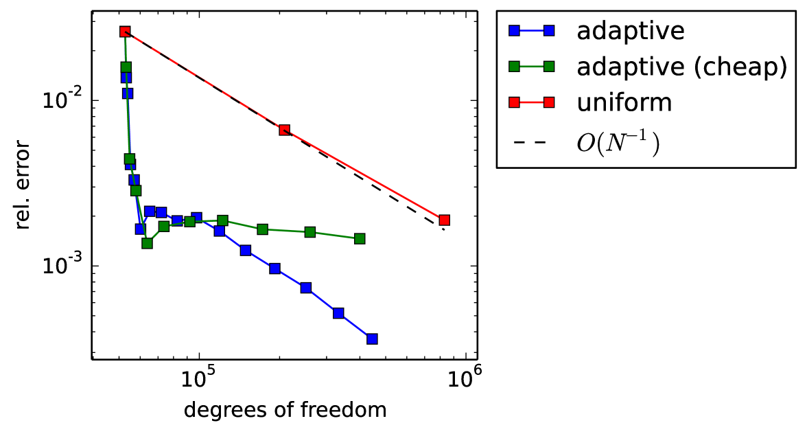
(a) Convergence of force: 2D

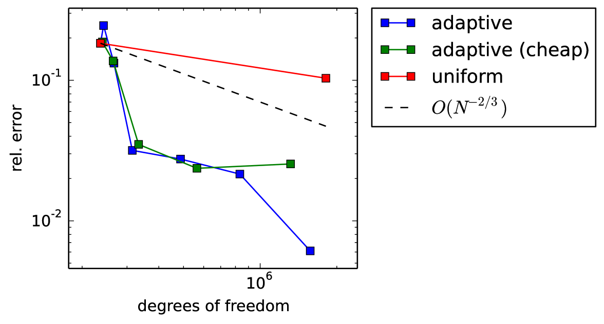
(b) Convergence of force: 3D

Figure 6: Performance of different refinement strategies with respect to the force (4) in axisymmetric 2D (left) and 3D (right). Starting from the same initial mesh, we compare the classical adaptive Algorithm 4, the cheap adaptive Algorithm 5 and uniform refinement of all elements. Shown is the error relative to a fine 2D reference solution, defined as

$${\rm error}:=\frac{|\boldsymbol{F}_{{\rm el},z}-\boldsymbol{F}_{{\rm el},z}^{{\rm ref}}|}{|\boldsymbol{F}_{{\rm el},z}^{{\rm ref}}|}+\frac{|\boldsymbol{F}_{{\rm drag},z}-\boldsymbol{F}_{{\rm drag},z}^{{\rm ref}}|}{|\boldsymbol{F}_{{\rm drag},z}^{{\rm ref}}|}.$$

We compare only the $z$-components of the forces since the radial components are zero by design in the axisymmetric formulation (the molecule sits on the central axis). The reason we sum absolute values of electrical and drag error components is to avoid a “lucky cancellation” that was observed in several data points and would make the errors shown in this figure unreliable.

In Figure 6, we compare the different refinement strategies proposed in Section 3.3, the classical goal-adaptive algorithm with extrapolation and the proposed cheaper variant without extrapolation, as well as uniform refinement as a baseline. Both in 2D (left) and 3D (right), the adaptive schemes are clearly superior to uniform refinement, especially in the first couple of steps when the error gets quickly reduced by about one order of magnitude. After that, however, the cheap estimator degrades in performance, while the classical estimator seems to enter an asymptotic phase where a well-defined convergence rate of is assumed, which can be heuristically derived from theory using a priori estimates.

Practically speaking, we see that both adaptive schemes make it possible to drive the approximation error of our main quantities of interest down to a few percent, in the full 3D problem, with a single CPU core on a desktop machine as used for creating Figure 6. In case the axisymmetric 2D formulation can be applied, even much lower tolerances can be achieved more quickly. Regarding the choice of adaptive algorithm, from our results we would recommend to stick with the more expensive Algorithm 4 (which is still cheap compared to solving the PNPS system). This algorithm does surprisingly well given that it only uses information from solutions to the linear Poisson-Boltzmann equation, and despite inexact discretization of the curved geometry. The cheaper variant (Algorithm 5) seems to capture the rough regions of interest during the first few refinement steps but may not be valid in the asymptotic limit.

4.4 Finite-sized vs. point-sized target molecule

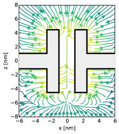
(a) Electric force

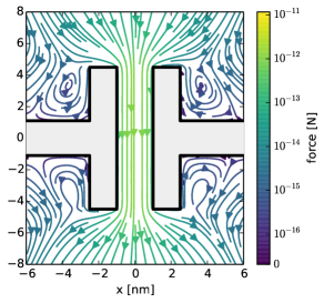
(b) Drag force

Figure 7: Streamline plots of PNPS force fields from the point-sized molecule model. The molecule has a radius $r=0.5$ nm and a negative total charge of $-q$.

After having obtained a good picture of the numerical accuracy of our adaptive PNPS solvers, we want to address the modeling question put forward in Section 2.4: whether to model the target molecule as finite-sized and explicitly part of the geometry or only implicitly (point-sized), i.e., simulate without molecule and only afterwards calculate the forces on a virtual molecule from the electric and flow fields.

The point-sized molecule approach – albeit less accurate – is computationally attractive, since the whole force field is obtained from a single simulation, while in the finite-sized approach one has to compute the force on a different mesh for every distinct molecule position. In Figure 7, we show the electric and hydrodynamic force fields obtained from the point-size model and an axisymmetric simulation.

Qualitatively, the following physical phenomena can be observed in Figure 7: As the molecule is negatively charged, and the applied electric field is pointing downwards, the net electrical force $\boldsymbol{F}_{\text{el}}$ inside the pore is in the upper direction (Fig. 7, left). On the other hand, the negative surface charge of DNA (which makes up the pore wall) leads to crowding of the pore by positive ions; the positive ions move downwards, causing electroosmotic drag $\boldsymbol{F}_{\text{drag}}$ in the downward direction (Fig. 7, right). From these two competing effects, it is a priori not clear whether the net force on the molecule will be upwards or downwards. Outside the pore, the molecule is repelled away by $\boldsymbol{F}_{\text{el}}$ due to the equally signed charges, which leads to an energy barrier for entering the pore from either direction.

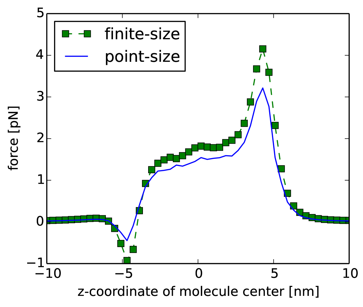
(a) Electric force along pore

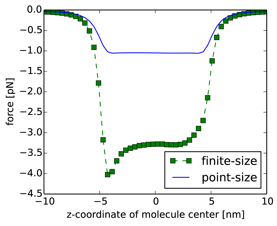
(b) Drag force along pore

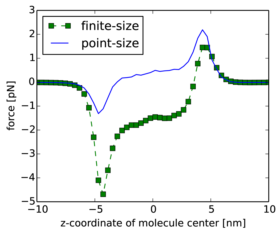
(c) Total force along pore

Figure 8: Force profiles along DNA nanopore, finite-size vs. point-size model. The $z$-component of forces is plotted along the central pore axis, where for the finite-size approach every data point corresponds to a distinct geometry and thus simulation; for the point-sized approach the whole curve is obtained from a single simulation. A negative total force in some region means that the target molecule is, on average, driven downward through the pore. In the point-size model, the magnitude of drag force is underestimated to such an extent that the net total force has a different direction than in the finite-size model.

Force profiles

In Figure 8, force profiles along the pore are compared for the finite- and point-size formulation. For the point-sized molecule, we calculate drag using Stokes’ law $\boldsymbol{F}_{\text{drag}}^{*}(x)=6\pi\eta r\boldsymbol{u}(x)$ which is valid for a particle in bulk water. As we can see (Fig. 8, center), this leads to a strong underestimation of drag force inside the pore. In the finite-size model, the drag force actually dominates the electric force by a factor $2$, but is weakened by a factor $3$–$4$ in the point-size model; so the net total force comes out in the wrong direction. For the electric force, agreement between both models looks more reasonable, yet the point-size model fails to capture an additional repelling force at the edges which can possibly be attributed to the dielectric self-energy of the molecule [11].

Improving the point-size model

Looking at Figure 8, it is clear that the point-size model could be improved a lot by simply scaling the drag force by a constant factor inside the pore. More generally, we propose to modify the calculation of the force on a point-sized molecule by using

$$\boldsymbol{F}^{*}(x)=\alpha(x)\boldsymbol{F}_{\text{el}}^{*}(x)+\beta(x)\boldsymbol{F}_{\text{drag}}^{*}(x).$$

Here, $\alpha(x)$ and $\beta(x)$ are corrective factors yet to be determined and $\boldsymbol{F}_{\text{el}}^{*}(x)$, $\boldsymbol{F}_{\text{drag}}^{*}(x)$ are the point-sized molecule forces given by (8) and (9). The corrections $\alpha$ and $\beta$ will be obtained by some parametrization of the finite-size model, for instance by evaluating the finite-size forces $\boldsymbol{F}_{\text{el}}(x)$ and $\boldsymbol{F}_{\text{drag}}(x)$ on a small number of points $x_{1},\ldots,x_{n}$ and constructing $\alpha$ and $\beta$ by interpolation to satisfy

$$\alpha(x_{i})=\frac{\boldsymbol{F}_{\text{el}}(x_{i})}{\boldsymbol{F}_{\text{el}}^{*}(x_{i})},\qquad\beta(x_{i})=\frac{\boldsymbol{F}_{\text{drag}}(x_{i})}{\boldsymbol{F}_{\text{drag}}^{*}(x_{i})},\qquad i=1,\ldots,n.$$

In this way we ensure $\boldsymbol{F}^{*}(x_{i})=\boldsymbol{F}(x_{i})$ at the interpolation points. The idea is that the expensive finite-size model has to be evaluated only at a few points instead of hundreds or thousands, since the rough overall shape of $\boldsymbol{F}^{*}$ is correctly determined by the point-size model. Thus we hope to get the best of both models, efficiency as well as accuracy.

For demonstration, we apply this approach – which we dub the hybrid-size model – using only a single interpolation point at the pore center. The resulting correction factor $\beta(x)$ to the drag force is shown in Figure 9(a), for molecules of different charges. We constructed $\beta$ so that is has the same (interpolated) value throughout the pore; outside the pore, we set $\beta=1$ (assuming that the point-size model is correct under bulk conditions), and in the transition region near the pore edges, we interpolate linearly between those two values. For $\alpha(x)$ the procedure is the same.

By using only one interpolation point, we deliberately ignore possible edge effects captured by the finite- but not the point-size model. Still, as shown in Figure 9(b), 9(c), this approach significantly improves on the pure point-size model for molecules of both positive and negative charge, with only twice the computational cost. This may be in part due to our specific nanopore geometry, which has a constant radius along the entire pore; but the approach is general enough to be applicable to irregularly shaped pore proteins such as $\alpha$-hemolysin, by using more than one interpolation point.

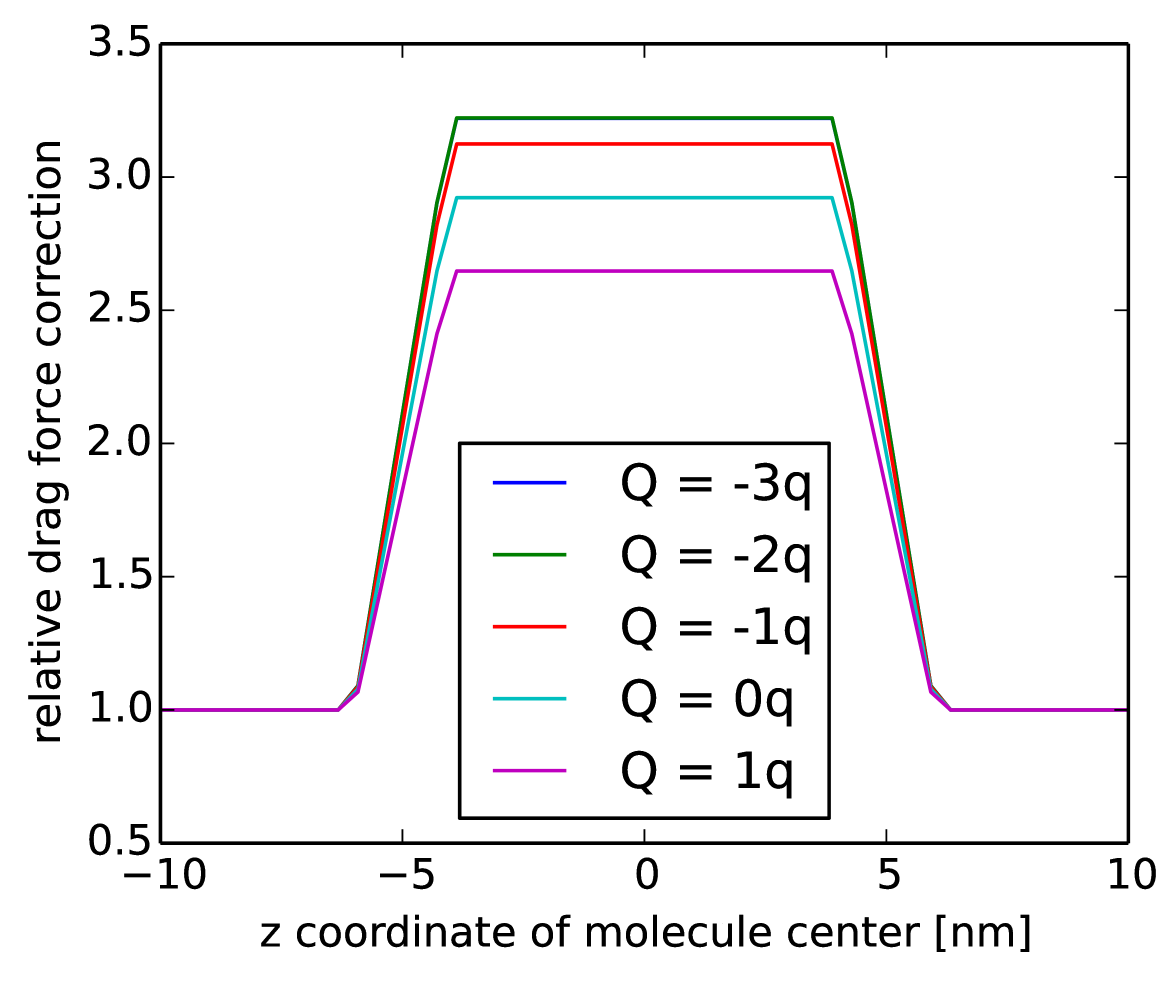
(a) Correction of drag force $\beta$(x) for different molecule charges

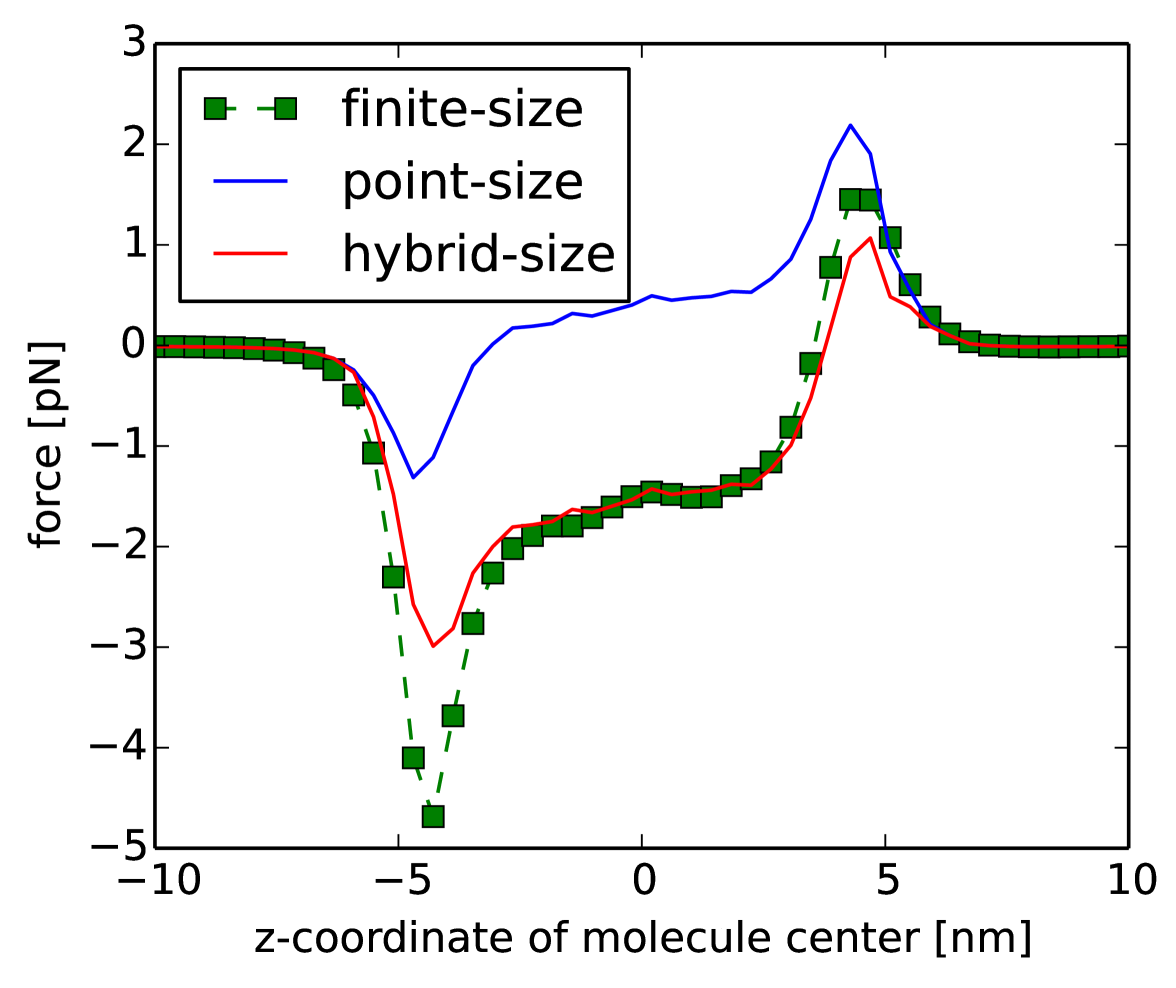
(b) Total force, molecule charge $-q$

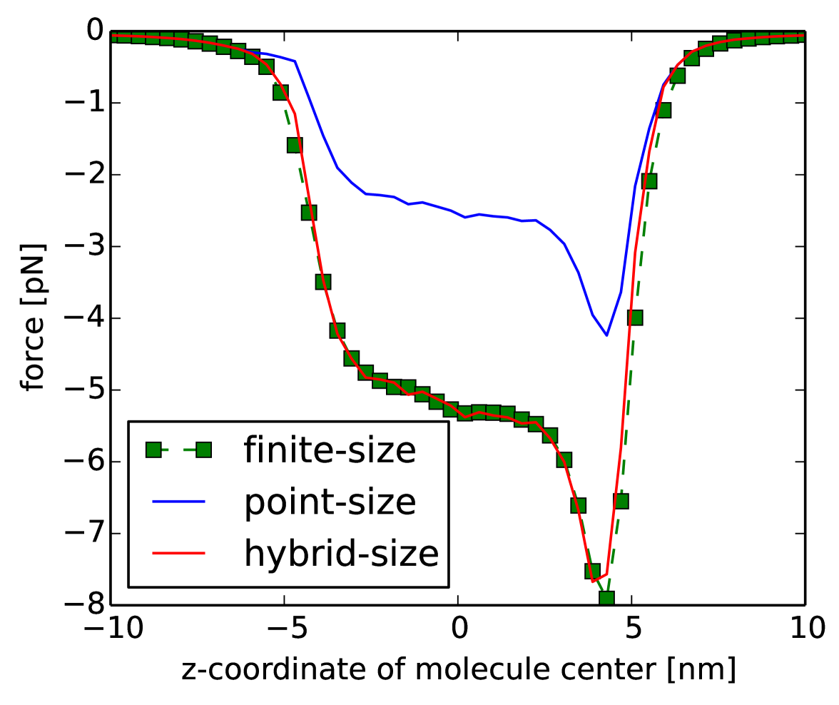
(c) Total force, molecule charge $+q$

Figure 9: Demonstration of the hybrid-size model for approximating the finite-size model with minimal computational effort. Left: Correction factor computed for the drag force, which measures by how much the finite-size model is underestimated by the point-size model. Center/right: Corrected force profiles for molecules with negative and positive unit charge, respectively.

Comparison of molecule flux

Finally, we want to provide a more succinct way of relating our three models (finite-, point- and hybrid-size). In the end, we are interested in how the PNPS force influences selectivity between different molecule species. Therefore, the single number that represents each model best is the flux of target molecules, i.e., the number of molecules translocating the pore in a given time interval. We model transport along the $z$-direction by a 1D diffusion equation $\frac{dc}{dt}=\frac{d}{dz}(-D\frac{dc}{dz}+\frac{D}{kT}Fc)$; the molecules start out in the upper reservoir and diffuse through the force field in the pore region. Details on the equation and how we solve it are given in Appendix A.3. The term inside the brackets $(-D\frac{dc}{dz}+\frac{D}{kT}Fc)$ is the flux density; multiplied by the crosssectional area of the pore, it gives the total molecule flux through the pore. We have computed the flux after a time of $1\mu{\rm s}$ for many different molecule charges and sizes, with results shown in Figure 10.

In Figure 10, looking at molecule fluxes from the finite-size model (green), we see that our sensor exhibits non-trivial selectivity between molecules of different charges. Strongly negatively charged molecules struggle to make their way through the pore against the direction of voltage bias. This is more pronounced for smaller molecules; for large molecules of radius $r=0.75$ nm, there is almost no differentiation, as the charge-agnostic drag force dominates. The latter effect is captured well by the hybrid-size model, but not by the uncorrected point-size model. However, the hybrid-size model as implemented with a single interpolation point underestimates the energy barrier at the pore entrance for large molecules of charge $-3q$, and therefore overstimates the flux there (Fig. 10, right). This effect vanishes for larger timescales, which is why we stopped after $1\ \mu{\rm s}$ to reveal the limitations of our proposed hybrid-size model.

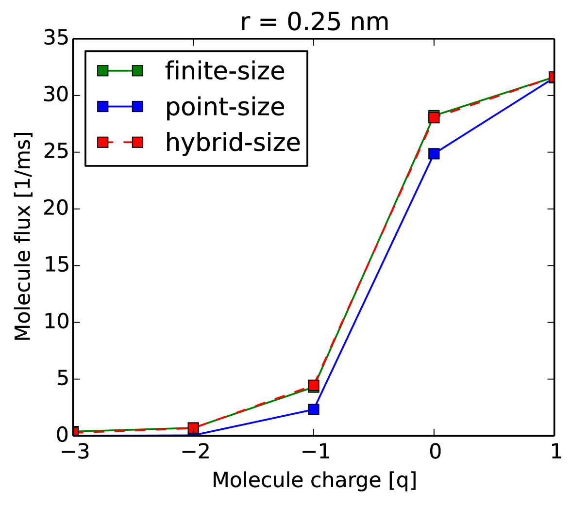
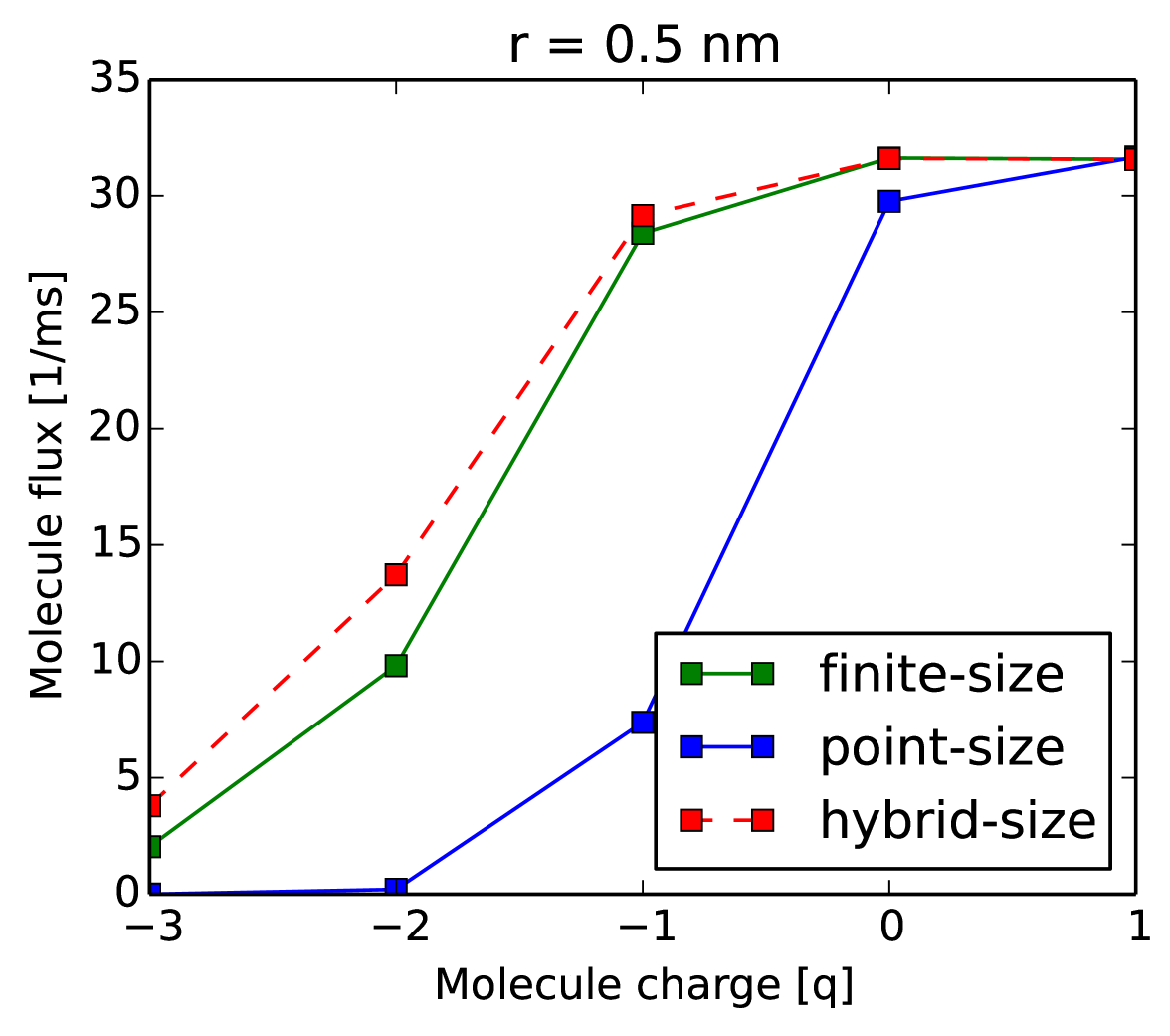
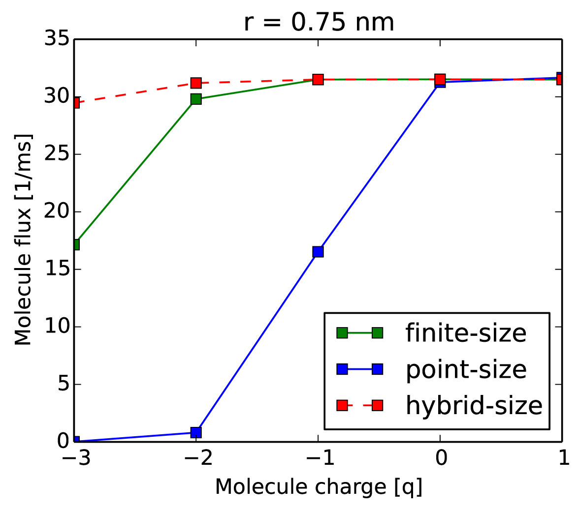
Figure 10: Molecule flux after $1\mu{\rm s}$ for different molecule charges and sizes and different models of the force. From left to right, the radii are $r=0.25$, $0.5$, $0.75$ nm. The point-size model does not match the results of the (expensive and more accurate) finite-size model. For most setups however, the (cheap) hybrid-size model comes relatively close.

5 Conclusion

We have implemented a 2D/3D finite element solver for the steady-state Poisson-Nernst-Planck-Stokes system for the simulation of nanopore sensors. To solve the nonlinear equations, we proposed three different schemes for linearization in an attempt to clarify the amount of system segregation that leads to the most efficient and robust solver. Two methods emerged as roughly equal candidates, with the pure fixed-point method being faster for small voltages and the hybrid method, if initialized from the Poisson-Boltzmann equation, better suited to work across a large range of voltages. For the fixed-point method, a new correction to the Poisson equation was proposed that prevents blow-up and – for small voltages – enables convergence in less than $10$ iterations without the need for damping.

The goal-adaptive mesh refinement schemes we proposed can efficiently allocate computational resources towards the prediction of output functionals. This proved indispensable to evaluate the electrophoretic force on particles in 3D with accuracies of over $99\%$ on non-HPC architectures. We experimented with a cheaper alternative to the goal-oriented error estimation procedure established in [2] by skipping the extrapolation step, but conclude that the extrapolation-based algorithm remains the more robust choice. Interestingly, we have shown that adaptivity can work in practice even if a radically simplified model is used to compute the error indicators. This gives a total speedup of roughly $50\%$, because we essentially save the effort to compute all the solutions on coarser meshes that are not needed in the end. The idea should be applicable to a variety of computational problems where model simplifications are available.

For the modeling of selectivity in nanopore sensors, we find that assuming a point-sized target molecule, although computationally attractive, severely reduces the predictiveness of our simulations. For practical applications, it is therefore recommended to model the molecule explicitly and calculate the force for each possible molecule position separately. However, if this is too expensive, a carefully calibrated hybrid model that we proposed may also capture most features of the force field and give results similar to the full finite-size model.

Appendix

A.1 Semi-analytical test problem

To validate our 2D and 3D solvers, we look at a simple model problem where the whole PNPS system can be reduced analytically to the solution of a scalar 1D boundary value problem. Since the 1D problem can be solved to high accuracy with negligible effort, it serves our purpose just as well as an exact analytical solution would. Unlike manifactured test problems often employed in academia, we do not introduce artificial right hand side terms. The problem actually describes, albeit simplified, a physically relevant situation: that of a nanopore where the pore length is large compared to the radius and the applied voltage is sufficiently low to have negligible influence on the ion distribution.

The domain is a plain cylindrical tube of radius $R=1$ nm and length $L=4$ nm and is meant to represent an inner part of the nanopore (far away from the pore entrances on either side); the only dielectric material is water. Using axial symmetry, we write the PNPS solutions as functions of the radial component $r$ and the height $z$. The exact potential is prescribed as

$$\phi(r,z)=U_{T}\phi^{*}(r)-E_{0}z,$$

where $E_{0}$ is a given constant external field strength, $U_{T}=kTq^{-1}$ is the thermal voltage and the dimensionless potential $\phi^{*}(r)$ solves a 1D radial Poisson-Boltzmann equation

$$\frac{1}{r}\frac{d}{dr}\left(r\frac{d\phi^{*}}{dr}\right)=\frac{1}{\lambda_{D}^{2}}\sinh(\phi^{*}).$$

Here $\lambda_{D}=\sqrt{\frac{\varepsilon kT}{2Fc_{0}q}}$ is the Debye length; the potential is subject to the boundary condition $U_{T}\frac{d\phi^{*}}{dr}(R)=\rho$ for a given constant surface charge density $\rho$. This equation is readily solved e.g. by 1D FEM.

The other unknowns depend only on $r$ and can all be obtained from $\phi^{*}(r)$: Ion concentrations are given by the Boltzmann factors

$$c^{\pm}(r)=c_{0}\exp\left(\mp\phi^{*}(r)\right)$$

for any given bulk concentration $c_{0}$; the velocity is of the form $\boldsymbol{u}=(0,0,u)^{T}$ with

$$u(r)=\frac{\varepsilon E_{0}}{\eta}U_{T}\left[\phi^{*}(r)-\phi^{*}(R)\right];$$

and the pressure is

$$p(r)=-2Fc_{0}U_{T}\cosh(\phi^{*}(r))+p_{0}$$

with an arbitrary constant $p_{0}$, which we fix by requiring $p(0)=0$. A mathematical derivation of this exact solution can be found in Appendix A.2.

Numerical results

We solve the problem both in 3D and in axisymmetric 2D variables. Dirichlet or Neumann boundary conditions are applied to match the exact solutions; we have tried to encode as little information about the exact solutions as possible into the boundary conditions. For instance, for the Stokes equation it suffices to enforce the usual no-slip condition $\boldsymbol{u}=0$ on the wall, the Neumann-type condition $n\cdot\nabla\boldsymbol{u}=0$ at the upper and lower ends, and the no pressure condition $p=0$ somewhere in the center. The numerical values used for the free parameters were $E_{0}=-100$ mV, $\rho=-0.05$ $\text{C}/\text{m}^{2}$ and $c_{0}=300$ $\text{mol}/\text{m}^{3}$, respectively. The Debye length, which determines the width of the double layer and thus the multiscale nature of the problem, is $\lambda_{D}=0.56$ nm in this case. Comparing this with the pore radius of $R=1$ nm, we see that we have posed ourselves a rather easy problem numerically (in the sense that a coarse mesh will suffice to resolve all features). Our test problem can be turned into a challenging benchmark problem by increasing the pore radius such that $R/\lambda_{D}$ is large.

In Fig. 11 we compare cross-sectional plots of ion concentrations and the velocity profile coming from the three different numerical formulations: the 1D Poisson-Boltzmann equation – which we take as the exact solution –, the axisymmetric 2D model and the full 3D PNPS system. We used a uniform mesh width of $h=0.1$ nm in these calculations, which corresponds to about $1$k mesh elements in 2D and $50$k in 3D. It is reassuring that the three results in Fig. 11 are almost indistinguishable.

For a quantitative assessment of the solver accuracy, we calculate the total ion current through the pore, defined as

$$J=F\int\left(j_{z}^{+}-j_{z}^{-}\right),$$

where $j_{z}^{\pm}$ is the $z$ component of the ion flux defined in (1); the integral is taken over any horizontal cross-section of the pore. In practice, it is more robust to average over many crosssections by taking a volume integral, which is what we do. The ion current involves the potential, both ion concentrations and the velocity and therefore provides a suitable measure of accuracy. In Fig. 12(a) we show the relative error of $J$ compared to the exact solution against number of iterations of our hybrid Newton/fixed-point scheme, with fixed mesh size $h=0.2$ nm. After about five iterations a converged state is reached where the error stops changing; at this point, the linearization error is dominated by the discretization error.

To study the discretization error, in Fig. 12(b) the mesh is refined uniformly starting from a coarse initial mesh, and the resulting error curve compared to the number of degrees of freedom is shown. Note that every data point in the latter figure corresponds to the final converged state of Fig. 12(a). Different asymptotic slopes for 2D and 3D arise as derived in Section 4.3, confirming that the error in $J$ is $O(h^{2})$. This provides a strong validation for the correctness of our implementation. More generally speaking, the results also indicate that for the current we should attain high numerical accuracy quite easily in simulations similar to this test problem, without any goal-specific adaptivity.

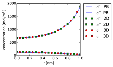
(a) Ion concentrations

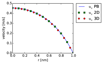
(b) Velocity profile

Figure 11: Cross-sectional plots for the analytical test problem with three different numerical methods: the 1D PB equation and the 2D and 3D PNPS solvers.

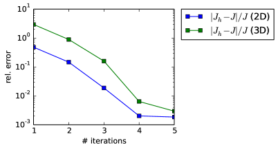
(a) Convergence with nonlinear iteration

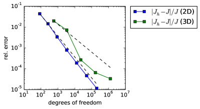
(b) Convergence with mesh refinement

Figure 12: Convergence to exact solution. The relative error is defined as $|J_{h}-J|/|J|$ where $J$ is the exact current from the 1D model and $J_{h}$ is the output of the PNPS solvers. 12(a) Error against number of iterations in the hybrid linearization scheme. 12(b) Error against degrees of freedom $N$ for uniform mesh refinement. The theoretical $N$ dependency is $O(N^{-1})$ in 2D and $O(N^{-2/3})$ in 3D, indicated by dashed lines.

A.2 Derivation of test problem

First, assume that the potential $\phi(r,z)$ is a superposition of a part resulting from a given constant external field $E_{0}$ in the $z$-direction and a part which depends only on the radius. Thus,

$$\phi(r,z)=\psi(r)-E_{0}z.$$

Second, the ion concentrations are assumed to depend only on $r$ and to be given by Boltzmann factors

$$c^{\pm}(r)=c_{0}\exp\left(\mp\frac{q\psi(r)}{kT}\right).$$

Third, for the Stokes equation we assume the velocity is of the form $\boldsymbol{u}=(0,0,u_{z})^{T}$ with $u_{z}=u_{z}(r)$ and pressure $p=p(r)$, i.e., the velocity field points only in the $z$-direction but is constant in this direction.

These three assumptions, which can be encoded in the boundary conditions, determine a solution to the PNPS system as follows. Since the second derivatives of the external part of the potential $-E_{0}z$ vanish and because of the assumed form of the ion concentrations, the Poisson equation reduces to a 1D Poisson-Boltzmann equation in radial direction

$$\varepsilon\frac{1}{r}\partial_{r}(r\partial_{r}\psi)=2Fc_{0}\sinh\left(\frac{q\psi}{kT}\right)$$

with Neumann boundary condition $\partial_{r}\psi(R)=\rho$ for some given (constant) surface charge density $\rho$. The permittivity $\varepsilon$ is constant since our domain only consists of fluid.

The Stokes equation splits into a $x$, $y$ part only for the pressure (since $u_{x}=u_{y}=0$) and a $z$ part only for the velocity (since $\partial_{z}p=0$),

$$\partial_{r}p = -F(c^{+}-c^{-})\partial_{r}\psi,$$ (20)

$$-\eta\frac{1}{r}\partial_{r}(r\partial_{r}u_{z}) = -F(c^{+}-c^{-})E_{0}.$$ (21)

Equation (20) can be solved by noting that the right hand side can be written as a derivative

$$-F(c^{+}-c^{-})\partial_{r}\psi=-2Fc_{0}\sinh\left(\frac{q\psi}{kT}\right)\partial_{r}\psi=\partial_{r}\left[-2Fc_{0}\frac{kT}{q}\cosh\left(\frac{q\psi}{kT}\right)\right],$$

which is equal to $\partial_{r}p$, thus yielding

$$p(r)=-2Fc_{0}\frac{kT}{q}\cosh\left(\frac{q\psi(r)}{kT}\right)+p_{0}$$

for some arbitrary constant $p_{0}$. For equation (21), we write on the other hand

$$-F(c^{+}-c^{-})=\varepsilon\frac{1}{r}\partial_{r}(r\partial_{r}\psi)$$

and obtain

$$\partial_{r}(r\partial_{r}u_{z})=-\frac{\varepsilon E_{0}}{\eta}\partial_{r}(r\partial_{r}\psi),$$

which combined with the no-slip condition $u(R)=0$ yields the solution

$$u(r)=\frac{\varepsilon E_{0}}{\eta}\left[\psi(R)-\psi(r)\right].$$

Finally, the form of these solutions can be simplified by writing the potential as $\psi(r)=\frac{kT}{q}\phi^{*}(r)$, where $\phi^{*}(r)$ is dimensionless.

A.3 Diffusion equation for molecule flux

We show how to compute the flux of target molecules for the results in Figure 10, Section 4.4. For simplicity, we model flux only in the $z$-direction. Given a force profile $F(z)$ which is obtained from the PNPS model (e.g. Fig. 8), the time-dependent diffusion equation for target molecules reads

$$j = -D\frac{dc}{dz}+\frac{D}{kT}Fc,$$ (22a)

$$\frac{dj}{dz} = \frac{dc}{dt}.$$ (22b)

Here, $c(z,t)$ is the molecule concentration; $j(z,t)$ is the molecule flux density; and $D(z)$ is the position-dependent diffusion coefficient. We solve this equation on the symmetric interval $|z|\leq 1\ \mu{\rm m}$, with $|z|\leq 4.5\ {\rm nm}$ defining the pore region. For the initial condition, we use

$$c(z,0)=\begin{cases}c_{0},&z>4.5\ \text{nm,}\\ 0,&\text{elsewhere,}\end{cases}$$

with $c_{0}=1\text{ mol}/\text{m}^{3}$. Thus, the molecules start out uniformly distributed in the upper reservoir, and will diffuse downwards through the pore region. At the reservoir boundaries $z=\pm 1\ \mu{\rm m}$, Neumann conditions $\frac{dj}{dz}=0$ are applied, modeling hard walls. The diffusion coefficient is modeled by a generalized Stokes-Einstein relation

$$D(z)=\frac{kT}{6\pi\eta r}d(z)\qquad\text{where }d(z)=\begin{cases}d_{r}<1&\text{in the pore,}\\ 1&\text{in bulk.}\end{cases}$$

Here, $r$ denotes the molecule radius. The reduced relative diffusivity $d_{r}$ inside the pore depends on $r$ and is taken from the tables in [46].

We solve (22) using backward Euler in time applied to a $P^{1}$ finite element space discretization on a uniform grid. For the results in Fig. 10, we used a grid spacing of $h=0.2$ nm ($10$k nodes), a timestep of $dt=10$ ns and stopped after $100$ steps or $t=1\ \mu{\rm s}$. The final-time downwards flux density $-j(\cdot,t)$ was averaged over the pore region and multiplied by the cross-sectional pore area $A=\pi(1{\rm nm})^{2}$ and the Avogrado constant $N_{A}$ to yield the molecule flux in numbers per second.

References

- Balay and et al. [2014] Balay, S., et al., 2014. PETSc users manual revision 3.5. Argonne National Laboratory (ANL).
-
Bangerth and Rannacher [2003]
Bangerth, W., Rannacher, R., 2003. Adaptive finite element methods for
differential equations. Birkhäuser.
URL http://www.springer.com/birkhauser/mathematics/book/978-3-7643-7009-1 -
Bayley [2015]
Bayley, H., 2015. Nanopore sequencing: From imagination to reality. Clinical
Chemistry 61 (1), 25–31.
URL http://www.clinchem.org/content/61/1/25.full -
Becker and Rannacher [2003]
Becker, R., Rannacher, R., jan 2003. An optimal control approach to a
posteriori error estimation in finite element methods. Acta Numerica
10 (January 2003), 1–102.
URL http://www.journals.cambridge.org/abstract_S0962492901000010 -
Burns et al. [2016]
Burns, J. R., Seifert, A., Fertig, N., Howorka, S., jan 2016. A biomimetic
DNA-based channel for the ligand-controlled transport of charged molecular
cargo across a biological membrane. Nature Nanotechnology advance on (2),
1–16.
URL http://dx.doi.org/10.1038/nnano.2015.279 -
Burns et al. [2013]
Burns, J. R., Stulz, E., Howorka, S., jul 2013. Self-assembled DNA nanopores
that span lipid bilayers. Nano Letters 13 (6), 2351–2356.
URL http://dx.doi.org/10.1021/nl304147f - Carstensen et al. [2014] Carstensen, C., Feischl, M., Page, M., Praetorius, D., 2014. Axioms of adaptivity. Computers and Mathematics with Applications 67 (6), 1195–1253.
-
Chen et al. [1995]
Chen, D. P., Eisenberg, R. S., Jerome, J. W., Shu, C. W., dec 1995.
Hydrodynamic model of temperature change in open ionic channels.
Biophysical Journal 69 (6), 2304–22.
URL http://www.sciencedirect.com/science/article/pii/S0006349595801013 - Coalson and Kurnikova [2005] Coalson, R. D., Kurnikova, M. G., 2005. Poisson-Nernst-Planck theory approach to the calculation of current through biological ion channels. IEEE Transactions on Nanobioscience 4 (1), 81–92.
- Comer and Aksimentiev [2012] Comer, J., Aksimentiev, A., 2012. Predicting the DNA sequence dependence of nanopore ion current using atomic-resolution brownian dynamics. Journal of Physical Chemistry C 116 (5), 3376–3393.
- Corry et al. [2003] Corry, B., Kuyucak, S., Chung, S.-H., 2003. Dielectric self-energy in Poisson-Boltzmann and Poisson-Nernst-Planck models of ion channels. Biophysical Journal 84 (6), 3594–3606.
- Deparis [2004] Deparis, S., 2004. Numerical Analysis of Axisymmetric Flows and Methods for Fluid-Structure Interaction Arising in Blood Flow Simulation. Ph.D. thesis, École Polytechnique Fédérale de Lausanne.
-
Dörfler [1996]
Dörfler, W., 1996. A convergent adaptive algorithm for Poisson’s
equation. SIAM Journal on Numerical Analysis 33 (3), 1106–1124.
URL http://epubs.siam.org/doi/abs/10.1137/0733054 -
Egwolf et al. [2010]
Egwolf, B., Luo, Y., Walters, D. E., Roux, B., mar 2010. Ion selectivity of
alpha-hemolysin with beta-cyclodextrin adapter. II. multi-ion effects studied
with grand canonical monte carlo/brownian dynamics simulations. Journal of
Physical Chemistry B 114 (8), 2901–2909.
URL http://www.pubmedcentral.nih.gov/articlerender.fcgi?artid=2843906&tool=pmcentrez&rendertype=abstract -
Erickson and Li [2002a]
Erickson, D., Li, D., mar 2002a. Influence of surface
heterogeneity on electrokinetically driven microfluidic mixing. Langmuir
18 (5), 1883–1892.
URL http://dx.doi.org/10.1021/la015646z -
Erickson and Li [2002b]
Erickson, D., Li, D., nov 2002b. Microchannel flow with patchwise
and periodic surface heterogeneity. Langmuir 18 (23), 8949–8959.
URL http://dx.doi.org/10.1021/la025942r -
Falgout and Yang [2002]
Falgout, R. D., Yang, U. M., 2002. hypre: A Library of High Performance
Preconditioners. Computational Science – ICCS 2002, 632–641.
URL http://link.springer.com/10.1007/3-540-47789-6 - Feischl et al. [2014] Feischl, M., Führer, T., Mitscha-Eibl, G., Praetorius, D., Stephan, E. P., 2014. Convergence of adaptive BEM and adaptive FEM-BEM coupling for estimators without h-weighting factor. Computational Methods in Applied Mathematics 14 (4), 485–508.
-
Feischl et al. [2016]
Feischl, M., Praetorius, D., van der Zee, K. G., 2016. An abstract analysis of
optimal goal-oriented adaptivity. SIAM Journal on Numerical Analysis 54 (3),
1423–1448.
URL http://dx.doi.org/10.1137/15M1021982 -
Freund [1993]
Freund, R. W., 1993. A Transpose-Free Quasi-Minimal Residual Algorithm for
Non-Hermitian Linear Systems. SIAM Journal on Scientific Computing 14 (2),
470–482.
URL http://epubs.siam.org/doi/abs/10.1137/0914029 - George et al. [1994] George, A., Liu, J., Ng, E., 1994. Computer Solution of Sparse Linear Systems. Prentice-Hall Series in Computational Mathematics. Prentice-Hall.
-
Geuzaine and Remacle [2009]
Geuzaine, C., Remacle, J. F., sep 2009. Gmsh: A 3-D finite element mesh
generator with built-in pre- and post-processing facilities. International
Journal for Numerical Methods in Engineering 79 (11), 1309–1331.
URL http://doi.wiley.com/10.1002/nme.2579 -
Ghosal [2006]
Ghosal, S., oct 2006. Electrophoresis of a polyelectrolyte through a
nanopore. Physical Review E 74 (4 Pt 1), 041901.
URL http://journals.aps.org/pre/abstract/10.1103/PhysRevE.74.041901 -
Gummel [1964]
Gummel, H. K., oct 1964. A Self-Consistent Iterative Scheme for
One-Dimensional Steady State Transistor Calculations. IEEE Transactions on
Electron Devices 11 (10), 455–465.
URL http://ieeexplore.ieee.org/lpdocs/epic03/wrapper.htm?arnumber=1473752 -
Heitzinger and Ringhofer [2011]
Heitzinger, C., Ringhofer, C., 2011. A transport equation for confined
structures derived from the Boltzmann equation. Communications in
Mathematical Sciences 9 (3), 829–857.
URL http://intlpress.com/site/pub/files/_fulltext/journals/cms/2011/0009/0003/CMS-2011-0009-0003-a008.pdf -
Howorka and Siwy [2012]
Howorka, S., Siwy, Z. S., jun 2012. Nanopores as protein sensors. Nature
Biotechnology 30 (6), 506–507.
URL http://dx.doi.org/10.1038/nbt.2264 -
Hughes and Franca [1987]
Hughes, T. J. R., Franca, L. P., nov 1987. A new finite element formulation
for computational fluid dynamics: VII. The stokes problem with various
well-posed boundary conditions: Symmetric formulations that converge for all
velocity/pressure spaces. Computer Methods in Applied Mechanics and
Engineering 65 (1), 85–96.
URL http://www.sciencedirect.com/science/article/pii/0045782587901848 - Jansson et al. [2013] Jansson, J., Hoffman, J., Degirmenci, C., 2013. Adaptive error control in finite element methods using the error representation as error indicator. Tech. rep., KTH Royal Institute of Technology.
-
Karatay et al. [2015]
Karatay, E., Druzgalski, C. L., Mani, A., may 2015. Simulation of chaotic
electrokinetic transport: Performance of commercial software versus
custom-built direct numerical simulation codes. Journal of Colloid and
Interface Science 446, 67–76.
URL http://www.sciencedirect.com/science/article/pii/S0021979714010510 -
Kerkhoven [1988]
Kerkhoven, T., 1988. On the Effectiveness of Gummel’s Method. SIAM Journal on
Scientific and Statistical Computing 9 (1), 48–60.
URL http://epubs.siam.org/doi/abs/10.1137/0909005 -
Keyser et al. [2010]
Keyser, U. F., van Dorp, S., Lemay, S. G., mar 2010. Tether forces in DNA
electrophoresis. Chemical Society Reviews 39 (3), 939–47.
URL http://www.ncbi.nlm.nih.gov/pubmed/20179816 -
Khodadadian and Heitzinger [2015]
Khodadadian, A., Heitzinger, C., 2015. A transport equation for confined
structures applied to the OprP, Gramicidin A, and KcsA channels. Journal of
Computational Electronics 14 (2), 524–532.
URL http://link.springer.com/article/10.1007/s10825-015-0680-6 -
Kuyucak et al. [2001]
Kuyucak, S., Andersen, O. S., Chung, S.-H., nov 2001. Models of permeation in
ion channels. Reports on Progress in Physics 64 (11), 1427–1472.
URL http://iopscience.iop.org/article/10.1088/0034-4885/64/11/202 - Langevin [1908] Langevin, P., 1908. Sur la theorie du mouvement Brownien. Comptes Rendus de l’Académie des Sciences (Paris) 146 (530-533), 530–533.
-
Laohakunakorn and Keyser [2015]
Laohakunakorn, N., Keyser, U. F., jul 2015. Electroosmotic flow rectification
in conical nanopores. Nanotechnology 26 (27), 275202.
URL http://www.ncbi.nlm.nih.gov/pubmed/26087132 - Logg et al. [2011] Logg, A., Mardal, K.-A., Wells, G. N., 2011. Automated Solution of Differential Equations by the Finite Element Method. Vol. 84. Springer Science & Business Media.
-
Lu et al. [2010]
Lu, B., Holst, M. J., Andrew McCammon, J., Zhou, Y. C., sep 2010.
Poisson-Nernst-Planck equations for simulating biomolecular
diffusion-reaction processes I: Finite element solutions. Journal of
Computational Physics 229 (19), 6979–6994.
URL http://www.pubmedcentral.nih.gov/articlerender.fcgi?artid=2922884&tool=pmcentrez&rendertype=abstract -
Lu et al. [2012]
Lu, B., Hoogerheide, D. P., Zhao, Q., Yu, D., jul 2012. Effective driving
force applied on DNA inside a solid-state nanopore. Physical Review E
86 (1), 011921.
URL http://journals.aps.org/pre/abstract/10.1103/PhysRevE.86.011921 -
Lu et al. [2007]
Lu, B., Zhou, Y. C., Huber, G. A., Bond, S. D., Holst, M. J., McCammon, J. A.,
oct 2007. Electrodiffusion: A continuum modeling framework for biomolecular
systems with realistic spatiotemporal resolution. Journal of Chemical
Physics 127 (13), 135102.
URL http://scitation.aip.org/content/aip/journal/jcp/127/13/10.1063/1.2775933 -
Maffeo et al. [2012]
Maffeo, C., Bhattacharya, S., Yoo, J., Wells, D., Aksimentiev, A., dec 2012.
Modeling and simulation of ion channels. Chemical Reviews 112 (12),
6250–6284.
URL http://dx.doi.org/10.1021/cr3002609 -
Mao et al. [2013]
Mao, M., Ghosal, S., Hu, G., jun 2013. Hydrodynamic flow in the vicinity of a
nanopore induced by an applied voltage. Nanotechnology 24 (24), 245202.
URL http://www.pubmedcentral.nih.gov/articlerender.fcgi?artid=3738177&tool=pmcentrez&rendertype=abstract -
Mao et al. [2014]
Mao, M., Sherwood, J. D., Ghosal, S., may 2014. Electro-osmotic flow through a
nanopore. Journal of Fluid Mechanics 749, 167–183.
URL http://www.journals.cambridge.org/abstract_S0022112014002146 -
Mardal and Winther [2011]
Mardal, K.-A., Winther, R., jan 2011. Preconditioning discretizations of
systems of partial differential equations. Numerical Linear Algebra with
Applications 18 (1), 1–40.
URL http://eprints.maths.ox.ac.uk/1499/ -
Metti et al. [2016]
Metti, M. S., Xu, J., Liu, C., feb 2016. Energetically stable discretizations
for charge transport and electrokinetic models. Journal of Computational
Physics 306, 1–18.
URL http://www.sciencedirect.com/science/article/pii/S0021999115007305 -
Noskov et al. [2004]
Noskov, S. Y., Im, W., Roux, B., oct 2004. Ion permeation through the
alpha-hemolysin channel: theoretical studies based on Brownian dynamics and
Poisson-Nernst-Plank electrodiffusion theory. Biophysical Journal 87 (4),
2299–2309.
URL http://www.pubmedcentral.nih.gov/articlerender.fcgi?artid=1304654&tool=pmcentrez&rendertype=abstract -
Paine and Scherr [1975]
Paine, P. L., Scherr, P., oct 1975. Drag coefficients for the movement of
rigid spheres through liquid-filled cylindrical pores. Biophysical Journal
15 (10), 1087–1091.
URL http://dx.doi.org/10.1016/S0006-3495(75)85884-X -
Prohl and Schmuck [2010]
Prohl, A., Schmuck, M., feb 2010. Convergent finite element discretizations of
the Navier-Stokes-Nernst-Planck-Poisson system. ESAIM: Mathematical
Modelling and Numerical Analysis 44 (3), 531–571.
URL http://www.esaim-m2an.org/10.1051/m2an/2010013 -
Quick and et al. [2016]
Quick, J., et al., 2016. Real-time, portable genome sequencing for Ebola
surveillance. Nature 530 (7589), 228–32.
URL http://www.nature.com/doifinder/10.1038/nature16996 -
Rognes and Logg [2013]
Rognes, M. E., Logg, A., apr 2013. Automated Goal-Oriented Error Control I:
Stationary Variational Problems. SIAM Journal on Scientific Computing
35 (3), C173–C193.
URL http://epubs.siam.org/doi/abs/10.1137/10081962X - Rubinstein [1990] Rubinstein, I., 1990. Electro-Diffusion of Ions. SIAM.
-
Sacco et al. [2015]
Sacco, R., Airoldi, P., Mauri, A. G., Jerome, J. W., sep 2015.
Three-Dimensional Simulation of Biological Ion Channels Under Mechanical,
Thermal and Fluid Forces. arXiv preprint, 1–38.
URL http://arxiv.org/abs/1509.07301 -
Schneider and Dekker [2012]
Schneider, G. F., Dekker, C., apr 2012. DNA sequencing with nanopores. Nature
Biotechnology 30 (4), 326–328.
URL http://dx.doi.org/10.1038/nbt.2181 -
Slotboom [1973]
Slotboom, J. W., aug 1973. Computer-Aided Two-Dimensional Analysis of Bipolar
Transistors. IEEE Transactions on Electron Devices 20 (8), 669–679.
URL http://ieeexplore.ieee.org/lpdocs/epic03/wrapper.htm?arnumber=1477384 -
Song et al. [1996]
Song, L., Hobaugh, M. R., Shustak, C., Cheley, S., Bayley, H., Gouaux, J. E.,
dec 1996. Structure of staphylococcal alpha-hemolysin, a heptameric
transmembrane pore. Science 274 (5294), 1859–66.
URL http://www.ncbi.nlm.nih.gov/pubmed/8943190 - van der Vorst [1992] van der Vorst, H. A., 1992. Bi-CGStab: a fast and smoothly converging variant of Bi-CG for the solution of nonsymmetric linear systems. SIAM Journal on Scientific and Statistical Computing 13 (2), 631–644.
-
van Dorp et al. [2009]
van Dorp, S., Keyser, U. F., Dekker, N. H., Dekker, C., Lemay, S. G., 2009.
Origin of the electrophoretic force on DNA in solid-state nanopores. Nature
Physics 5 (5), 347–351.
URL http://dx.doi.org/10.1038/nphys1230 -
Vlassiouk et al. [2008a]
Vlassiouk, I., Smimov, S., Siwy, Z., aug 2008a. Nanofluidic ionic
diodes. Comparison of analytical and numerical solutions. ACS Nano 2 (8),
1589–1602.
URL http://dx.doi.org/10.1021/nn800306u -
Vlassiouk et al. [2008b]
Vlassiouk, I., Smirnov, S., Siwyt, Z., jul 2008b. Ionic
selectivity of single nanochannels. Nano Letters 8 (7), 1978–1985.
URL http://dx.doi.org/10.1021/nl800949k - Wei et al. [2012] Wei, G.-W. W., Zheng, Q., Chen, Z., Xia, K., jan 2012. Variational multiscale models for charge transport. SIAM Review 54 (4), 699–754.