Quasinormal Modes and Thermodynamics of Linearly Charged BTZ Black holes in Massive Gravity in (Anti)de Sitter Space Time

Abstract

In this work we study the Quasi Normal Modes(QNMs) under massless scalar perturbations and the thermodynamics of linearly charged BTZ black holes in massive gravity in the (Anti)de Sitter((A)dS) space time. It is found that the behavior of QNMs changes with the massive parameter and also with the charge of the black hole. The thermodynamics of such black holes in the (A)dS space time is also analyzed in detail. The behavior of specific heat with temperature for such black holes gives an indication of a phase transition that depends on the massive parameter and also on the charge of the black hole.

1 Introduction

Einstein’s General Theory of Relativity(GTR) helped us to understand the dynamics of the universe. But there are some fundamental issues that could not be addressed in GTR eref1 and several attempts are being made to modify the GTR to find solutions to these fundamental issues. GTR is a theory based on massless gravitons with two degrees of freedom. A way of modifying GTR essentially implies giving mass to the graviton and in the present study we consider massive gravity. The attempts to modify GTR resulted in the so called ‘Alternative Theories of Gravity’1 . Theories concerning the breaking up of Lorentz invariance and spin had been explored in depth2 . The first attempt towards constructing a theory of massive gravity was done by Fierz and Pauli3 in 1939. Only by 1970s researchers showed interests in this formulation. van Dam and Veltman4 and Zhakharov5 in 1970 showed that a theory of massive gravity could never resemble GTR in the massless limit and this is known as vDVZ discontinuity. Later Vainshtein6 proposed that the linear massive gravity can be recovered to GTR through the ‘Vainshtein Mechanism’  at small scales by including non-linear terms in the hypothetical massive gravity action. But this model suffers from a pathology called ‘Boulware-Deser’(BD) ghost and was ruled out on the basis of solar system tests7 . Later a class of massive gravity was proposed by de Rham, Gahadadze and Tolley called ‘dRGT massive gravity’  that evades the BD ghost8 ; 9 . In this theory the mass terms were produced by a reference metric. A class of black hole solutions in the dRGT model and their thermodynamic behavior were studied later10 ; 11 ; 12 . Vegh13 proposed another type of massive gravity theory. This theory was similar to dRGT except that the reference metric was a singular one. Using this theory he showed that graviton behaves like a lattice and showed Drude peak. This theory was found to be ghost-free and stable for arbitrary singular metric.

It was Hawking14 who first showed that black holes thermally radiate and calculated its temperature. Thereafter the thermodynamics of black holes got wide acceptance and interests among researchers. The question of thermal stability is one of the important aspects of black hole thermodynamics15 ; 16 . The thermodynamics and phase transition shown by black holes have been largely explored for almost all space times17 ; 18 ; 19 ; 20 and references cited therein. In the realm of massive gravity also, the thermodynamics and phase transitions have been studied for different black hole space time21 ; 22 .

Recently there has been a growing interest in the asymptotically Anti de Sitter(AdS) spacetimes. The black hole solution proposed by Banados-Teitelboim-Zanelli (BTZ) in $(2+1)$ dimensions deal with asymptotically AdS space time and has got well defined charges at infinity, mass, angular momentum and makes a good testing ground especially when one would like to go beyond the asymptotic flatness23 . Another interesting aspect of the black hole solution is related to the AdS/CFT (Conformal Field Theory) correspondence. In $(2+1)$ dimensions, the BTZ black hole solution is a space time of constant negative curvature and it differs from the AdS space time in its global properties24 . The thermodynamic phase transitions and area spectrum of the BTZ black holes are studied in detail25 ; 26 ; 27 . Also, the charged BTZ black hole solutions are studied for the phase transition in Ref.28 ; 29 .

Another important aspect of a black hole is its Quasi Normal Modes (QNMs). QNMs can be found out as a solution to the perturbed field equation corresponding to the scalar, gravitational and electromagnetic perturbations of black hole space time. It comes out as a natural response to these perturbations. The existence of QNMs was first found by Visweshwara30 and attempts were made to find out QNMs for different space times. QNMs of black holes were first numerically computed by Chandrasekhar and Detweiler31 . It was Cardoso and Lemos32 who first calculated the exact QNMs of the BTZ black holes. They have found out both analytical and numerical solutions to the BTZ black hole perturbation for non-rotating BTZ black holes. It is interesting to note that they got exact analytical solutions to the wave equation that made BTZ an important space time where one can prove or disprove the conjectures relating to QNMs, critical phenomena or area quantization.

Electromagnetic field can be a good choice of source for getting deep insights into the 3 dimensional massive gravity. In this paper the QNMs, the associated phase transition and thermodynamics of BTZ black hole in massive gravity in the presence of Maxwell’s field has been studied. The paper is organized as follows: In section $2$ the QNMs of a linearly charged BTZ black holes in massive gravity are studied for different values of the massive parameter and charge for de Sitter and Anti de Sitter space-times. The behavior of quasi normal frequencies and phase transition are also dealt with. Section $3$ deals with the thermodynamics of such black holes. The influence of the massive parameter and charge of the black hole on the various thermodynamic factors are studied. Section $4$ concludes the paper.

2 Quasi normal modes of a linearly charged BTZ black hole in massive gravity

In this section, we first look into the perturbation of black hole space time by a scalar field. For a linearly charged black hole, the Einstein-Maxwell action in $(2+1)$ dimension is given by33 ,

$$S_{EM}=\frac{1}{16\pi G}\int d^{3}x\sqrt{-g}\left[R+\frac{2}{l^{2}}-4\pi GF_{\mu\nu}F^{\mu\nu}\right],$$ (1)

where $R$ is the Ricci scalar, $F_{\mu\nu}=\partial_{\mu}A_{\nu}-\partial_{\nu}A_{\mu}$ is the Faraday tensor, $A_{\mu}$ is the gauge potential, and $F^{\mu\nu}F_{\mu\nu}$ is the Maxwell invariant. The action given above can be generalized to include the massive gravity for the de Sitter space time as34 ,

$$\begin{split}S&=\frac{-1}{16\pi}\int d^{3}x\sqrt{-g}[R+2\Lambda+L(\mathcal{F})+\\ &\,\,\,\,\,\,m^{2}\sum_{i}^{4}c_{i}\mathcal{U}_{i}(g,f)],\end{split}$$ (2)

where $\mathcal{F}=F^{\mu\nu}F_{\mu\nu}$, $L$ is an arbitrary Lagrangian of electrodynamics, $\frac{1}{l^{2}}=\Lambda$, the cosmological constant in the de Sitter (dS) space time, $\mathcal{U}_{i}$ is the effective potential, $m$ is the massive parameter and $c_{i}$s are constants. Varying $(2)$ with respect to the metric $g_{\mu\nu}$, we can obtain the gravitation field equation as,

$$G_{\mu\nu}+\Lambda g_{\mu\nu}-\frac{1}{2}g_{\mu\nu}L(\mathcal{F})-2L_{\mathcal{F}}F_{\mu\rho}F^{\rho}_{\nu}+m^{2}\mathcal{K}_{\mu\nu}=0,$$ (3)

where,

$G_{\mu\nu}=R_{\mu\nu}-\frac{1}{2}g_{\mu\nu}R,$ $L_{\mathcal{F}}=\frac{dL(\mathcal{F})}{d\mathcal{F}}$, $\mathcal{K}^{\mu}_{\nu}=\sqrt{g^{\mu\alpha}f_{\alpha\nu}},$

and,

$$\begin{split}\mathcal{K}_{\mu\nu}&=\frac{-c_{1}}{2}(\mathcal{U}g_{\mu\nu}-\mathcal{K}_{\mu\nu})-\frac{c_{2}}{2}(\mathcal{U}_{2}g_{\mu\nu}-2\mathcal{U}_{1}\mathcal{K}_{\mu\nu}+\\ &2\mathcal{K}_{\mu\nu}^{2})-\frac{-c_{3}}{2}(\mathcal{U}_{3}g_{\mu\nu}-4\mathcal{U}_{3}\mathcal{K}_{\mu\nu}+\\ &12\mathcal{U}_{2}\mathcal{K}_{\mu\nu}^{2}-24\mathcal{U}_{1}\mathcal{K}_{\mu\nu}^{3}+24\mathcal{K}_{\mu\nu}^{4}).\end{split}$$ (4)

To obtain static charged black hole solution we consider the $3$ dimensional metric,

$$ds^{2}=-f(r)dt^{2}+f^{-1}(r)dr^{2}+r^{2}d\theta^{2}.$$ (5)

To get an exact solution for this metric, the following ansatz is employed13 ,

$$f_{\mu\nu}=diag(0,0,c^{2}h_{ij}),$$ (6)

where $c$ is a positive constant. One of the solutions after proper rescaling leads to the metric function in the dS space as33 ; 34 ,

$$f(r)=\Lambda r^{2}-m_{0}-2Q\ln{\frac{r}{\alpha}}+m^{2}cc_{1}r,$$ (7)

where $m_{0}$ is related to the mass of the black hole, $Q$ is the charge parameter, $\alpha$ is an arbitrary constant and $c_{1}$ is a constant. For an Anti de Sitter space, $\Lambda$ will take negative values. From the metric function, it can be understood that the contribution of the massive term depends on the sign of $c_{1}$. In this Section, we look into the behavior of QNMs of the linearly charged BTZ black hole with metric function given by $(7)$. A massless scalar field perturbation in this space time satisfies the Klein-Gordon equation,

$$\frac{1}{\sqrt{-g}}\frac{\partial}{\partial x^{a}}\left((g^{ab}\sqrt{-g}\frac{\partial}{\partial x^{b}}\right)\Phi=0,\\$$ (8)

which on expanding gives,

$$\frac{1}{f(r)}\frac{\partial^{2}\Phi}{\partial t^{2}}-\frac{\partial}{\partial r}f(r)\frac{\partial\Phi}{\partial r}-\frac{1}{r^{2}}\frac{\partial^{2}\Phi}{\partial\phi^{2}}=0.$$ (9)

The metric function $f(r)$ is given by $(7)$. To separate the angular variables, we make use of the ansatz,

$$\Phi=\frac{R(r)}{r}e^{-i\omega t}e^{im_{l}\phi},$$ (10)

where $\omega$ is the frequency, $m_{l}$ is the angular momentum quantum number. Using the above ansatz, the Klein-Gordon equation can be re-written as,

$$\frac{d^{2}R}{dr^{2}}+\frac{f^{\prime}(r)}{f(r)}\frac{dR}{dr}+\left[\frac{\omega^{2}}{f(r)^{2}}-\frac{(\frac{m_{l}^{2}}{r^{2}}-\frac{2Q}{r^{2}}+\frac{cc_{1}m}{r})}{f(r)}\right]R=0.$$ (11)

Quasi normal modes are in going waves at the event horizon and outgoing waves at the cosmological horizon, leading to the boundary condition,

$$R\rightarrow\begin{cases}e^{i\omega x},&\text{as }x\rightarrow\infty\\ e^{-i\omega x},&\text{as }x\rightarrow-\infty\end{cases}$$ (12)

Making a variable change $r\rightarrow 1/\xi$, the wave equation becomes,

$$\frac{d^{2}R}{d\xi^{2}}+\frac{p^{\prime}}{p}\frac{dR}{d\xi}+\left[\frac{\omega^{2}}{p^{2}}-\frac{2Q+\frac{2\Lambda}{\xi^{2}}-\frac{cc_{1}m}{\xi}-m_{l}^{2}}{p}\right]R=0,$$ (13)

where,

$$p = M\xi^{2}-cc_{1}m\xi+2Q\xi^{2}\ln{(\frac{1}{\alpha\xi})}+\Lambda,$$ (14)

$$p^{\prime} = 2(M-Q)\xi-cc_{1}m+4Q\xi\ln{(\frac{1}{\alpha\xi})}.$$ (15)

The wave equation given by $(13)$ has got the singularities at the event horizon and at an outer horizon. In order to solve the wave equation, the singularities have to be scaled out. Here, we first scale out the divergent behavior at the outer horizon and then re-scale to avoid the event horizon. To scale out the divergence at outer horizon, we take35 ,

$$R(\xi)=e^{i\omega\xi}u(\xi),$$ (16)

where,

$$e^{i\omega\xi}=(\xi-\xi_{1})^{\frac{i\omega}{2\kappa_{1}}}(\xi-\xi_{2})^{\frac{i\omega}{2\kappa_{2}}},$$ (17)

and,

$$\kappa_{i}=\frac{1}{2}\frac{\partial f}{\partial r}\mid r\rightarrow r_{i},$$ (18)

is the surface gravity at each horizon. The master equation then will take the form,

$$pu^{\prime\prime}+(p^{\prime}-2i\omega)u^{\prime}-\left(2Q-\frac{2\Lambda}{\xi^{2}}-\frac{cc_{1}m}{\xi}-m_{l}^{2}\right)u=0$$ (19)

This can be viewed as,

$$u^{\prime\prime}=\lambda_{0}(\xi)u^{\prime}+s_{0}(\xi)u,$$ (20)

with,

$$\lambda_{0} = -\frac{(p^{\prime}-2i\omega)}{p},$$ (21)

$$s_{0} = \frac{\left(2Q-\frac{2\Lambda}{\xi^{2}}-\frac{cc_{1}m}{\xi}-m_{l}^{2}\right)}{p}.$$ (22)

We employ the Improved Asymptotic Iteration Method (Improved AIM) explained in Ref.36 ; 37 ; 38 . The coefficients are found out upto $(n+2)^{th}$ derivative of $u$. It is assumed that when $n$ is large the ratio of the derivatives, $\frac{u^{n+2}}{u^{n+1}}=\frac{\lambda_{n-1}}{\lambda_{n}}$ converges to a constant value, $\alpha$. This makes the quantization condition given by,

$$\lambda_{n}(x)s_{n-1}(x)-\lambda_{n-1}(x)s_{n}(x)=0,$$ (23)

a possible one. It can be seen from $(21)$ that $\lambda_{0}$ contains the quasi normal frequencies. So, the quantization condition given by $(23)$ can be used to determine the quasinormal frequencies of the black hole.

Table 1: QNMs of linearly charged BTZ black hole for different values of the massive parameter for dS space time with $Q=0.25$

	$m=1$		$m=1.05$		$m=1.1$
$\Lambda$	$\omega=\omega_{R}+\omega_{I}$	$\Lambda$	$\omega=\omega_{R}+\omega_{I}$	$\Lambda$	$\omega=\omega_{R}+\omega_{I}$
0.05	1.10826 - 0.11372 i	0.13	2.34196 - 0.20795 i	0.19	4.17236 - 1.06710 i
0.06	1.11679 - 0.12335 i	0.15	2.44520 - 0.20739 i	0.21	4.27438 - 1.24924 i
0.07	1.12571 - 0.13415 i	0.17	2.54513 - 0.20066 i	0.23	4.36708 - 1.46493 i
0.08	1.13484 - 0.14622 i	0.19	2.63890 - 0.19441 i	0.25	4.44633 - 1.71966 i
0.09	1.14390 - 0.15966 i	0.21	2.72810 - 0.19347 i	0.27	4.50586 - 2.02037 i
0.10	1.15262 - 0.17447 i	0.21	2.72810 - 0.19347 i	0.28	4.52540 - 2.19059 i
0.11	1.57071 - 0.17563 i	0.22	2.77213 - 0.19538 i	0.29	0.54837 - 2.25384 i
0.12	1.57561 - 0.17204 i	0.23	2.81604 - 0.19882 i	0.30	0.50212 - 2.32018 i
0.13	1.58260 - 0.16856 i	0.25	2.90460 - 0.20967 i	0.31	0.45065 - 2.39119 i
0.14	1.59172 - 0.16559 i	0.27	2.99477 - 0.22423 i	0.32	0.39409 - 2.46833 i
0.15	1.60312 - 0.16277 i	0.29	3.08568 - 0.24039 i	0.33	0.33391 - 2.55151 i
0.16	1.61655 - 0.16277 i	0.31	3.25912 - 0.27670 i	0.34	0.26958 - 2.63657 i

In Table $1$ we list the Quasi normal frequencies of the black hole in the de Sitter space time for $m=1$, $m=1.05$ and $m=1.1$ for different values of the cosmological constant. We have used the parameter values $Q=0.25$, $m_{l}=1$, $\alpha=1$, $c=1$ and $c_{1}=1$. In the numerical calculations we have used $15$ iterations. It is observed that the behavior of the quasi normal frequencies change after a particular $\Lambda$ value. This change in behavior is shown in the table by a horizontal line as a separator. This sudden change in behavior happens at $\Lambda=0.1$ for $m=1$, at $\Lambda=0.21$ for $m=1.05$ and at $\Lambda=0.28$ for $m=1.1$. The variation of the QNMs with $\Lambda$ is shown in Fig. $1$.

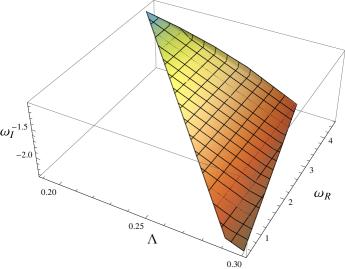
Figure 1: The behavior of QNMs with $\Lambda$ for $m=1.1$

The behavior of the QNMs for $m=1,0.05$ and $1.1$ given by Table $1$ are plotted in Fig. $2$.

Figure 2: QNM behavior for linearly charged BTZ black hole for the massive parameter value $m=1,1.05,1.1$. The sudden change in the slope can be treated as an indicative of a possible phase transition.

From the figures it can be clearly seen that the slope of the curve changes suddenly at some transition point for $m=1,1.05,1.1$. This behavior can be treated as a clear indication of a phase transition. However for the same values of the constant parameters this phase transition occurs at different values of $\Lambda$ for the different $m$ values. The higher the value of $m$, the larger the value of $\Lambda$ at which the phase transition occurs.

Table 2: QNMs of linearly charged BTZ black holefor different values of the massive parameter for dS space time with $Q=0.35$

	$m=0.9$		$m=0.95$		$m=1.0$
$\Lambda$	$\omega=\omega_{R}+\omega_{I}$	$\Lambda$	$\omega=\omega_{R}+\omega_{I}$	$\Lambda$	$\omega=\omega_{R}+\omega_{I}$
0.09	.898571 - .0783066i	0.05	1.16072 - .0686295i	0.01	1.68971 - .172263i
0.10	.901026 - .0798863i	0.06	1.18398 - .0690504i	0.015	1.69779 - .581786i
0.11	.902855 - .0851571i	0.07	1.20614 - .0630027i	0.02	1.70293 - .198065i
0.12	.902565 - .0947457i	0.08	1.21651 - .0514301i	0.025	1.70506 - .214255i
0.13	1.03909 - .107478i	0.09	1.21431 - .0415960i	0.03	1.70405 - .232616i
0.14	1.01865 - .0859070i	0.10	1.20180 - .0347956i	0.04	1.69178 - .27573i
0.15	1.00159 - .0683552i	0.11	1.17941 - .0303883i	0.05	1.66379 - .327079i
0.16	.983281 - .0666629i	0.12	1.14639 - .0274678i	0.06	1.61649 - .386106i
0.17	.961166 - .0464981i	0.13	1.10110 - .0251206i	0.07	1.54442 - .451769i
0.18	.933873 - .0396936i	0.14	1.04093 - .0224859i	0.08	1.43902 - .521872i

In Table $2$, we have shown the Quasi normal frequencies for $Q=0.35$ for $m=0.9$, $m=0.95$ and $m=1.0$ with the parameter values $m_{l}=c=c_{1}=1$. The behavior of these QNMs are shown in Figure $3$. Just like in the case where $Q=0.25$, here also there is a sudden change in the slope of the curve after a particular $\Lambda$ indicating that of a phase transition.

Figure 3: QNM behavior for linearly charged BTZ black hole for dS spece time with $Q=0.35$ for the massive parameter value $m=0.9,0.95,1.0$. The sudden change in the slope can be treated as an indicative of a possible phase transition.

Thus for both values of $Q$ the black hole shows phase transition. We can see that for the value $m=1.0$ the phase transition happens at a different value of $\Lambda$ compared to $Q=0.25$ and $Q=0.35$ cases.

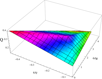
Figure 4: Variation of QNMs with charge $Q$ for the dS space time

In Table $3$ we show the QNMs for an AdS space time for the parameter values $Q=0.1$, $\alpha=1$, $c=1$, $c_{1}=1$ and $m=1,1.05,1.1$. From the table, it can be observed that the $\omega_{R}$ and $\omega_{I}$ continuously decrease and after reaching a particular point $(\Lambda=0.12)$, the real part suddenly increases and then continuously decrease whereas the imaginary part continues to decrease. This jump can be treated as an indication of an inflection point.

Table 3: QNMs of linearly charged BTZ black hole for different values of the massive parameter for AdS space time with $Q=0.1$

	$m=1.0$		$m=1.05$		$m=1.1$
$\Lambda$	$\omega=\omega_{R}+\omega_{I}$	$\Lambda$	$\omega=\omega_{R}+\omega_{I}$	$\Lambda$	$\omega=\omega_{R}+\omega_{I}$
-0.06	1.83077 - 5.78701 i	-0.05	1.39873 - 7.68495 i
-0.07	1.70014 - 5.33444 i	-0.06	1.29210 - 7.27705 i	-0.04	0.75408 - 9.41718 i
-0.08	1.53828 - 4.92198 i	-0.07	1.14457 - 6.93423 i	-0.05	0.63741 - 9.08170 i
-0.09	1.34563 - 4.54476 i	-0.08	0.95604 - 6.62556 i	-0.06	0.48892 - 8.73203 i
-0.10	1.11762 - 4.20206 i	-0.09	0.72592 - 6.35819 i	-0.07	0.21318 - 8.39613 i
-0.11	0.84041 - 3.89983 i	-0.95	0.58718 - 6.23146 i
-0.12	0.48197 - 3.66706 i	-0.10	0.40624 - 6.12793 i
-0.13	0.81813 - 4.06506 i	-0.11	1.57334 - 7.10865 i	-0.08	2.18254 - 10.2207 i
-0.135	0.75562 - 3.41486 i	-0.13	1.12639 - 5.99601 i	-0.09	1.44272 - 10.1043 i
-0.14	0.32251 - 2.91165 i	-0.14	0.86214 - 5.07753 i	-0.10	1.41871 - 9.40952 i

The $\omega_{R}$ versus $\omega_{I}$ is plotted in Fig. $3$. It can be seen from the figure that there is no drastic change in the slope and the behavior of the QNMs are same. Hence it can be inferred that there will be no phase transition.

Figure 5: QNM behavior for linearly charged BTZ black hole with charge Q =0.1 for AdS space time for the massive parameter value $m=1,1.05,1.1$. The dotted line represents the behavior of QNMs after the inflection point. The behavior of QNMs are seen to be the similar in the plots. There is no much difference in the slope of the curves

In Table $4$ we have calculated the QNMs for the AdS space time for the charge $Q=0.25$. Fig. $6$ shows the behavior of quasi normal frequencies for the above case. It can be seen that there is a sudden change in slope of the curve after reaching a particular $\Lambda$ indicating a phase transition. For $Q=0.1$ the AdS black hole space time did not show any phase transition behavior but for $Q=0.25$ it is found to be showing a phase transition behavior. Hence, it can be inferred that the phase transition behavior depends on the charge $Q$.

Table 4: QNMs of linearly charged BTZ black hole for different values of the massive parameter for AdS space time with $Q=0.25$

	$m=0.95$		$m=1.0$		$m=1.05$
$\Lambda$	$\omega=\omega_{R}+\omega_{I}$	$\Lambda$	$\omega=\omega_{R}+\omega_{I}$	$\Lambda$	$\omega=\omega_{R}+\omega_{I}$
0.01	.292587 - 9.19482i	0.13	.820054 - 4.96149i	0.29	1.01098 - .0351877i
0.02	.772162 - 8.39220i	0.15	.431983 - 3.38060i	0.31	1.02868 - .0148701i
0.03	.844245 - 7.75702i	0.17	.00879691 - .0348464i	0.32	1.04119 - .00215093i
0.04	.820904 - 7.24016i	0.19	1.72429 - .0660172i	0.33	1.62431 - .102106i
0.05	.759655 - 6.75177i	0.20	1.73419 - .0561830i	0.34	1.62400 - .083530i
0.07	.551068 - 5.89321i	0.21	1.74461 - .043151i	0.35	1.61905 - .067770i
0.09	.390010 - 4.86350i	0.22	1.75581 - .0330092i	0.36	1.60957 - .060276i
0.11	.243717 - 3.77402i	0.23	1.76769 - .0186321i

Figure 6: QNM behavior for linearly charged BTZ black hole for $Q=0.25$ the massive parameter value $m=0.95,1.0,1.05$.

Now, it would be interesting to check the variation of QNMs with $Q$. Table $5$ shows the variation of quasi normal frequencies with charge $Q$ for dS space time. It can be seen that the behavior of quasi normal frequency changes frequently. The phase transition behavior is highly dependent on the charge. The phase does not remain the same for a wide range of charge and hence phase transition is found to happen frequently over a range of charges.

Table 5: Table showing the variation of QNMs with $Q$ for dS space time

Q	$\omega$
0.15	4.47348 - 0.19884 i
0.20	4.33915 - 0.108836 i
0.25	0.0930679 - 0.0668980 i
0.30	1.54638 - 0.132502 i
0.35	1.68971 - 0.172263 i
0.40	0.0325096 - 0.466834 i

The variation of QNMs with charge for the AdS case is shown in Table $6$.

Table 6: Table showing the variation of QNMs with $Q$ for the AdS space

Q	$\omega$
0.05	1.12930 - 9.66585 i
0.10	1.14048 - 9.54589 i
0.15	2.42998 - 12.8629 i
0.20	3.49176 - 14.0316 i
0.25	3.64711 - 13.9835 i
0.30	0.294699 - 9.56518 i
0.35	0.557735 - 9.42807 i
0.40	0.792729 - 9.21181 i
0.45	0.940783 - 9.04476 i
0.50	1.03930 - 8.88485 i

It can be seen that compared to the dS case, phase transition does not happen frequently, ie., the phases remain the same for most of the values of charge and a transition happens only for certain small range of charge values. This behavior can be seen in Fig $7$.

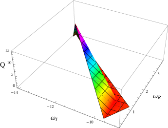
Figure 7: Variation of QNMs with charge $Q$ for AdS space time

3 Thermodynamics of the black hole

In this section, we study the thermodynamics of the linearly charged BTZ black hole in the (Anti)de Sitter space time in massive gravity. The mass of the black hole, $m_{0}$, is given by the solution of the condition $f(r)|_{r\rightarrow r_{H}}=0$ as,

$$m_{0}=m^{2}cc_{1}r_{H}+\Lambda r_{H}^{2}-2Q\ln{(\frac{r_{H}}{\alpha})}.$$ (24)

The temperature of the black hole is given by $\frac{1}{4\pi}f^{\prime}(r)|_{r\rightarrow r_{H}}$ which gives,

$$T=\frac{cc_{1}m^{2}}{4\pi}-\frac{Q}{2\pi r_{H}}+4Pr_{H}.$$ (25)

where $P=\frac{\Lambda}{8\pi}$. Finally, the entropy is evaluated from the expression $S=\int_{0}^{r_{H}}\frac{1}{T}\frac{\partial m_{0}}{\partial r}dr$ which gives,

$$S=4\pi r_{H}.\\$$ (26)

Then the equation of state, $P(V,T)$ can be obtained from the expression for temperature, $(25)$, as,

$$P=\frac{Q}{8\pi r_{H}^{2}}+\frac{-cc_{1}m^{2}+4\pi T}{16\pi r_{H}}.$$ (27)

For an $(n+2)$ dimensional massive gravity, the volume is given by39 , $V=(\frac{\partial H}{\partial P})_{S,Q}=\frac{V_{n}}{n+1}r^{n+1}$. With, $n=1$, the calculation gives the horizon radius in terms of its volume as, $r_{H}=(\frac{V}{8\pi})^{1/2}$.

To specify the phase transition it will be useful to introduce the Gibbs free energy as a Legendre transformation of enthalpy as,

$$G=H-TS,$$ (28)

where $H$ is the enthalpy, $T$ is the temperature given by $(25)$ and $S$ is the entropy given by $(26)$. We use the black hole mass $m_{0}$ as the enthalpy since $H\equiv m_{0}$ rather than the internal energy of the gravitational system21 . Substituting $(24)$, $(25)$ and $(26)$ in $(28)$, we get an expression for the Gibbs free energy as,

$$G(T,\Lambda)=2Q+\Lambda r_{H}^{2}-2Q\ln{(\frac{r_{H}}{\alpha})}.\\$$ (29)

Fig. $8$ shows the variation of Gibbs free energy with temperature plotted using $(25)$ and $(29)$. Top of the figure shows the G-T plot for $P=\frac{\Lambda}{8\pi}=0.001$. It can be seen that the upper branch which lies in the positive Gibbs free energy region moves towards the lower branch which lies in the ‘positive temperature-negative Gibbs free energy’  region which indicates a possible phase transition. The bottom plot shows variation of G with T for $P=-0.001$. The plot lies in the positive Gibbs free energy region and shows a cusp like behavior.

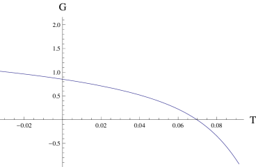
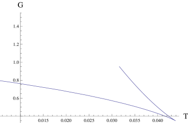
Figure 8: Variation of Gibbs free energy with temperature for the dS space time (top) and AdS space tome (bottom).

Fig. $9$ shows the variation of pressure, $P$ and temperature, $T$ with the horizon radius, $r_{H}$, for fixed values of temperature and pressure respectively. Top of the Fig. $9$, shows the variation of temperature with $r_{h}$ given by $(25)$ for the pressure values $P=-0.003$, $-0.002,$ $-0.001,$ $0.001,$ and $0.002$. The bottom of the Fig. $9$ shows the variation of pressure with $r_{h}$ given by $(27)$ for the fixed values of temperature, $T=-0.3,$ $-0.2,$ $-0.1,$ $0.1,$ and $0.2$.

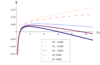
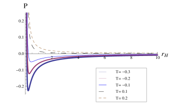
Figure 9: Top : Variation of $T$ with $r_{H}$. Bottom : Variation of $P$ with $r_{H}.$

More details regarding the phase transition can be extracted form the entropy of the system. The temperature-entropy relation would be worth looking at. For that the expression for $r_{H}$ derived from $(26)$ is substituted into $(25)$ so that we get an expression relating the entropy and temperature as,

$$T=-\frac{2Q}{S}+\frac{2\pi cc_{1}m^{2}+\Lambda\,S}{8\pi^{2}}.$$ (30)

Fig. $10$ shows the $S-T$ plots for the values $\Lambda=0.1$ and $\Lambda=-0.1$, with the parameter values $m_{0}=c=c_{1}=1$, $\alpha=1$, $Q=0.25$ and $m=1$. It can be seen that $S$ remains positive only for a small range of temperature and both of them show phase transition behavior.

Figure 10: The variation of thermal entropy with temperature for the $\Lambda=0.1$(top) and $-0.1$(bottom) in dS space time

Now, in order to study the stability of the phases or the feasibility of the above phase transitions, it may be worth looking at the behavior of specific heat with temperature. If the behavior of heat capacity indicates that as the temperature varies the heat capacity makes a transition from negative values to positive values the system undergoes a phase transition. Negative heat capacity represents unstable state while positive value of specific heat implies a stable state. The specific heat is given by,

$$C_{Q}=\frac{T}{(\frac{\partial T}{\partial S})_{Q}},$$ (31)

which from $(26)$ and $(30)$ leads to,

$$C_{Q}=2\pi r_{h}\frac{\left(-2Q+r_{h}\left(m^{2}+2r_{h}\Lambda\right)\right)}{Q+r_{h}^{2}\Lambda}.$$ (32)

The plots of specific heat versus temperature for $\Lambda=0.1$ and $\Lambda=-0.1$ is given in Fig. $11$ for the parameter values $m=c=c_{1}=1$ and $Q=0.25$ . From the plot it can be clearly understood that for $\Lambda=0.1$, the specific heat changes from negative to positive values indicating a phase transition from unstable to stable configuration. For $\Lambda=-0.1$, from the figure we can say that it somewhat shows a phase transition behavior however, it is observed that for given constant parameter values, the black holes in AdS space time show this phase transition behavior only for a very small range of $\Lambda$ values whereas in dS space time it shows phase transition for a wide range of $\Lambda$ values.

Figure 11: Figure showing the variation of specific heat with temperature for $\Lambda=0.1$(top) and $\Lambda=-0.1$(bottom).

It would also be worth noting that the variation of the behavior of specific heat with $Q$. For this, we have plotted variation of specific heat with temperature for $Q=0.1,0.25,0.5,0.6$ for dS space time; the other parameters remaining the same and is shown in Fig $12$.

Figure 12: The variation of thermal entropy with temperature for $Q=0.1,0.25,0.5,0.6$ respectively from top left in dS space time

It can be seen that upto $Q=0.5$ it shows a phase transition and then after reaching $Q=0.6$, it no more shows any phase transition. Also it is found that above this value no phase transition is observed.

The variation of the behavior of specific heat with $Q$ for the AdS space time for the values $Q=0.1,0.25,0.3,0.4$ is shown in FIg $13$.

Figure 13: The variation of thermal entropy with temperature for $Q=0.1,0.25,0.3,0.4$ respectively from top left in AdS space time

It can be seen that for $Q=0.1$ it does not show any phase transition and upto $Q=0.3$ it shows a phase transition and then after reaching $Q=0.4$, it no more shows any phase transition. Also it is found that above this value no phase transition is observed. From this it can also be concluded that AdS space time shows phase transition only for a small range of $Q$ when compared with the dS space time.

4 Conclusion

In this paper we have calculated the QNMs for a linearly charged BTZ black hole in massive gravity. The values of the parameters are so chosen that in the metric function, the massive parameter dominates. It is found that in the de Sitter space time as the cosmological constant $\Lambda$ is increased, the quasi normal frequencies varied continuously and then after reaching a particular value of $\Lambda(=0.1)$, their behavior is found to be abruptly changing afterwards. This is shown in the $\omega_{I}-\omega_{R}$ plot where there is a drastic change in the slope of the curve after a particular value of $\Lambda$. This can be seen as a strong indication of a possible phase transition occurring in the system. When the massive parameter $m$ is increased, a similar behavior is found but the $\Lambda$ at which the change of behavior of QNMs is found to be shifted to a higher value$(\Lambda=0.28)$. Also, it can be inferred that the variation of the massive parameter will only alter the point at which the phase transition happens. For different values of $Q$ the phase transition occurs for different values of $\Lambda$.

The QNMs for an (Anti)de Sitter space time is also calculated and the behavior of their quasi normal frequencies are analyzed. For $Q=0.1$ the behavior of QNMs showed an inflection point but no phase transition. However for $Q=0.25$ it showed a phase transition. Thus it is seen that the phase transition behavior is found dependent on $Q$ for the AdS case. It is also observed by studying the variation of QNMs with $Q$ that AdS space time shows phase transition only for certain limited ranges of $Q$ compared to the dS case.

The thermodynamics of such black holes in the dS space is then looked into. The behavior of specific heat showed phase transition for the dS case for a wide range of $Q$ whereas for AdS space time phase transition is shown only for a limited range of $Q$.

References

- (1) Salvatore Capozziello and Mariafelicia De Laurentis, Phys. Rep. 509,167(2011)(arXiv:1108.6266)
- (2) Timothy Clinton,Phys.Rep.513,1(2012)
- (3) Mattingly, D.,Liv.Rev.Rel.8,lrr-2005-5(2005)
- (4) Fierz, M. and Pauli, W.,Proc. R.Soc.Lond.Ser.A. 173, 211232(1939)
- (5) van Dam H.and Veltman M.J.G., Nucl.Phys.B, 22,397(11970)
- (6) Zakharov V. I.,JETP Lett.,12,312(1970)
- (7) Vainshtein, A. I.,Phys. Lett. B.39,393(1972)
- (8) Boulware,D.G.and Deser S., Phys. Rev. D6,3368(1972)
- (9) de Rham, C., Gabadadze, G. and Tolley, A.J.,Phys.Rev.Lett.106,231101(2011)
- (10) Volkov, M. S., Class. Quantum Grav. 30 184009 (2013)
- (11) Kodama H. and Arraut I,Prog.Theor.Exp.Phys.023E0(2014)(arXiv:1312.0370)
- (12) S. G. Ghosh, L.Tannukij and P. Wongjun, Eur. Phys. J. C. 76 (2016) 119.
- (13) P.Prasia and V.C.Kuriakose, Gen. Rel.Gravit.48,89(2016)
- (14) D.Vegh,CERN-PH-TH/2013-357(2013) [arXiv:1301.0537].
- (15) Hawking,S.W.and Page,D.N., Commun. Math. Phys. 87,577(1983)
- (16) P.C.W.Davies,Rep. Prog. Phys. 41,1313(1978)
- (17) Gross D.J.,Perry M.J. and Yaffe L.G., Phys. Rev.D25,330(1982)
- (18) S.Carlip arXiv 1410.1486
- (19) Brian P Dolan.,Class. Quantum Grav.28,125020(2011)
- (20) K.Ghaderi and B.Malakolkalami., Nucl. Phys.B,903,10(2016)
- (21) Jishnu Suresh, R. Tharanath, Nijo Varghese and V.C. Kuriakose, Eur. Phys. J C., 74, 2819(2014)
- (22) Fabio Capelaa and Peter G. Tinyakov., JHEP 1104:042(2011) (arXiv:1102.0479)
- (23) R.G. Cai, Y. P. Hu, Q. Y. Pan and Y. L. Zhang, Phys. Rev. D.91,024032(2015)
- (24) M. Banados, C. Teitelboim, and J. Zanelli, Phys. Rev. Lett.69,1849 (1992).
- (25) M. Banados, M. Henneaux,C. Teitelboim and J. Zanelli, Phys. RevD.48,1506 (1992).
- (26) Norman Cruz and Samuel Lepe, Phys. Lett.B,593,235(2004)
- (27) Mariano Cadoni and Maurizio Melis, Found. Phys. 40,638(2010) (arXiv:0907.1559)
- (28) A. Chamblin, R. Emparan, C. Johnson, and R. Myers, Phys.Rev. D60,064018(1999)
- (29) M. Cadoni, M. Melis and M.R. Setare, Class. Quantum Grav. 25,195022(2008)
- (30) M.R. Setare and H. Adami, Phys. RevD, 91, 104039(2015)
- (31) Vishveswara, C.V., Nature 227, 936(1970)
- (32) S.Chandrasekhar and S. Detweiler, Proc. R. Soc. London A344,441(1975).
- (33) V. Cardoso and J. P. S. Lemos, Phys. Rev. D 63, 124015(2001)
- (34) Debaprasad Maity et al., Nucl. Phys. B839:526,(2010) (arXiv:0909.4051v2).
- (35) S. H. Hendi, B. Eslam Panah and S. Panahiyan, JHEP 05,029(2016)(arXiv:1604.00370v1)
- (36) Moss I. G. and Norman J. P., Class. Quant. Grav.19,2323(2002)
- (37) Ciftci H.,Hall R.L. and Saad, N.,Phys. Lett. A,340,388(2005)
- (38) Cho H.T.,Cornell, A.S., Jason, D., Huang, T.R.and Wade N., Adv. Math. Phys.,doi:10.1555/2012/281705(2012)
- (39) Cho H.T.,Cornell, A.S.,Jason, D. and Wade N., Class. Quantum Grav.27,155004(2010)
- (40) J Xi, L Cao and Y-P Hu, Phys. RevD.,91,124033(2015)