Effects of interactions on periodically driven dynamically localized systems

Abstract

It is known that there are lattice models in which non-interacting particles get dynamically localized when periodic $\delta$-function kicks are applied with a particular strength. We use both numerical and analytical methods to study the effects of interactions in three different models in one dimension. The systems we have considered include spinless fermions with interactions between nearest-neighbor sites, the Hubbard model of spin-1/2 fermions, and the Bose Hubbard model with on-site interactions. We derive effective Floquet Hamiltonians up to second order in the time period of kicking. Using these we show that interactions can give rise to a variety of interesting results such as two-body bound states in all three models and dispersionless few-particle bound states with more than two particles for spinless fermions and bosons. We substantiate these results by exact diagonalization and stroboscopic time evolution of systems with a few particles. We derive a pseudo-spin-1/2 limit of the Bose Hubbard system in the thermodynamic limit and show that a special case of this has an exponentially large number of degenerate eigenstates of the effective Hamiltonian. Finally we study the effect of changing the strength of the $\delta$-function kicks slightly away from perfect dynamical localization; we find that a single particle remains dynamically localized for a long time after which it moves ballistically.

I Introduction

Periodically driven quantum systems have been studied extensively for many years as they exhibit a wide variety of interesting phenomena. These include the coherent destruction of tunneling grossmann91 ; kayanuma94 , the generation of defects mukherjee08 ; mukherjee09 , dynamical freezing das10 , dynamical saturation russomanno12 and localization alessio13 ; bukov14 ; nag14 ; nag15 ; agarwala16 , dynamical fidelity sharma14 , edge singularity in the probability distribution of work russomanno15 and thermalization lazarides14a (for a review see Ref. dutta15, ). There have also been proposals of Floquet driving of graphene by radiation gu11 ; kitagawa11 ; morell12 ; sentef15 , Floquet topological insulators and the generation of topologically protected edge states kitagawa10 ; lindner11 ; jiang11 ; trif12 ; gomez12 ; dora12 ; cayssol13 ; liu13 ; tong13 ; rudner13 ; katan13 ; lindner13 ; kundu13 ; basti13 ; schmidt13 ; reynoso13 ; wu13 ; manisha13 ; perez1 ; perez2 ; perez3 ; reichl14 ; manisha14 ; some of these aspects have been experimentally studied kitagawa12 ; rechtsman13a ; rechtsman13b ; rechtsman14 ; tarruell12 ; jotzu14 .

The effects of interactions between electrons in periodically driven systems have received much attention in recent times Eckardt05 ; Rapp12 ; Zheng14 ; Greschner14 ; lazarides14b ; rigol14 ; ponte15a ; lazarides14c ; ponte15b ; Eckardt15 ; BukovPRL16 ; lazarides14d ; keyser16 ; else16a ; else16b . It has been shown that a sinusoidal perturbation of the Hubbard model can lead to coherent destruction of tunneling, creation of gauge fields, and density-dependent tunneling Itin15 . The effects of interactions on Floquet topological insulators have been examined in Ref. mikami16, . It has been shown that interactions can lead to a chaotic and topologically trivial phase in the periodically driven Kitaev model su16 . The impact of such driving on the stability of a bosonic fractional Chern insulator has been investigated Raciunas16 . Interestingly some of these systems have been realized experimentally demonstrating correlated hopping in the Bose Hubbard model Meinert2016 and many-body localization BordiaPRL16 ; Bordia16 , and realizing bound states for two particles in driven photonic systems Mukherjee16 .

A particularly interesting phenomenon which can arise due to driving is dynamical localization. Here the particles become perfectly localized in space due to periodic driving of some parameter in the Hamiltonian. Examples of systems showing dynamical localization include driven two-level systems grossmann91 , classical and quantum kicked rotors chirikov81 ; fishman82 ; ammann98 ; tian11 ; nieuwenburg12 , the Kapitza pendulum kapitza51 ; broer04 , and bosons in an optical lattice horstmann07 . It has been shown that remnants of dynamical localization may survive even in the presence of strong disorder Roy15 .

In this paper, we will study the effects of periodic driving on a number of systems with interacting particles. The motivation for this is as follows. Suppose we consider a system without any interactions and subject it to a periodic driving which dynamically localizes the particles. This means that the effective Floquet Hamiltonian of the system has no kinetic energy; for instance, in a tight-binding model, the effective hopping amplitude is zero. We now add interaction terms to the Hamiltonian. We may then expect that the properties of the system will be entirely dominated by these terms. Systems which are dominated by interactions often have interesting ground states, such as fractional quantum Hall systems and fractional Chern insulators in general regnault11 ; sheng11 ; neupert11 ; wang11 ; tang11 . We will therefore look at the effects of interactions on systems which are dynamically localized in the absence of interactions. We will consider only one-dimensional models here although many of our results can be easily generalized to higher dimensions. As will become clear, new effective hopping terms are generated by the interactions; these lead to dispersing two-particle bound states and dispersionless bound states with more than two particles. We will mainly study systems with a few particles rather than a finite density of particles. However, for the Bose Hubbard model we will study the eigenstates of the effective Hamiltonian of a large system with a finite particle density in a particular limit.

The plan of our paper is as follows. In Sec. II, we will show that particles moving in a bipartite lattice with a non-interacting Hamiltonian can become dynamically localized if periodic $\delta$-function kicks with a particular strength given by $\alpha=\pi$ are applied to the sublattice potential. (The advantage of looking at periodic $\delta$-function kicks, in contrast to sinusoidal driving nag15 , is that the problem can be studied analytically to a large extent nag14 ; dasgupta14 ; agarwala16 ). The dynamical localization becomes clear when we view the system stroboscopically, at intervals of time given by $2T$, where $T$ is the time period of the kicking. We find that the effective Hamiltonian which evolves the system for time $2T$ is exactly zero for this non-interacting problem. In Sec. III, we will show how a generic model with interactions can be studied by computing the effective Hamiltonian. This Hamiltonian can be derived as an expansion in powers of $T$, and we will carry out the expansion up to order $T^{2}$. In Sec. IV, we will consider a model of spinless fermions with nearest-neighbor interactions in one dimension. After deriving the effective Hamiltonian to order $T^{2}$, we will show that the system has two branches of two-body bound states; these states move slowly if $T$ is small in appropriate units. We will also show that there are bound states with three or more particles; these objects have zero dispersion and do not move. We will demonstrate these results both analytically and numerically. In Sec. V, we will consider the Hubbard model in one dimension, namely, a spin-1/2 model with on-site interactions. After deriving the effective Hamiltonian, we will show analytically and numerically that this has two branches of two-body bound states which are spin singlets. In Sec. VI, we will study the Bose Hubbard model with on-site interactions in one dimension. We will derive the effective Hamiltonian and show that there are again two dispersing branches of two-particle bound states and dispersionless bound states with more than two particles. We will then consider a limit in which the interactions have a two-fold degenerate ground state on each site. After defining a pseudo-spin-1/2 on each site, we derive an effective Hamiltonian for the system. This contains both two-spin and three-spin interactions. For a special case (one in which particle occupation numbers zero and 1 are degenerate on each site), we show that a class of degenerate eigenstates of the effective Hamiltonian can be found exactly and the number of such states grows exponentially with the system size. In Sec. VII, we will study the effects of two kinds of perturbations on dynamical localization when there are no interactions. First, we study what happens if the strength of the $\delta$-function kicks, $\alpha$, is slightly different from $\pi$. We show that a particle remains dynamically localized for a long time which is of the order of $1/|\pi-\alpha|$. After that time the particle begins to move ballistically with a maximum velocity which is of the order of $|\pi-\alpha|$. Second, we study what happens if $\alpha=\pi$ but there is some randomness in the nearest-neighbor hoppings. In this case, we find that a particle remains dynamically localized if we view at intervals of time $2T$. We end in Sec. VIII with a summary of our main results and some directions for future work.

II Dynamical Localization

In this section we will consider a general non-interacting Hamiltonian on a bipartite lattice which respects the sublattice symmetry. We will show that such a system exhibits dynamical localization when periodic $\delta$-function kicks with a particular strength are applied to the sublattice potential.

We consider a Hamiltonian on a bipartite lattice given by

$$H_{NI}~{}=~{}\sum_{ij}~{}t_{ij}~{}(c^{\dagger}_{iA}c_{jB}+H.c.),$$ (1)

where $i$ and $j$ represent site labels residing on the two sublattices $A$ and $B$. We now apply periodic $\delta$-function kicks to the sublattice potential as follows: the kicking part of the Hamiltonian, $H_{K}$, is given by

$$H_{K}~{}=~{}\alpha~{}\sum_{n=-\infty}^{\infty}\delta(t-nT)~{}\left(\sum_{i}n_{iA}~{}-~{}\sum_{j}n_{jB}\right),$$ (2)

where $n_{iA}=c^{\dagger}_{iA}c_{iA}$ and $n_{jB}=c^{\dagger}_{jB}c_{jB}$ denotes the number of particles on site $i$ on sublattice $A$ and site $j$ on sublattice $B$. We define the total number of particles on the two sublattices as

$$N_{A}~{}=~{}\sum_{i}n_{iA}~{}~{}~{}~{}{\rm and}~{}~{}~{}~{}N_{B}~{}=~{}\sum_{j}n_{jB}.$$ (3)

Without the kick the time evolution operator is given by

$$U_{NI}~{}=~{}e^{-iH_{NI}T}.$$ (4)

(We will set $\hbar=1$ in this paper). The time evolution corresponding to the kick is

$$U_{K}=e^{-i\alpha~{}(N_{A}~{}-~{}N_{B})}.$$ (5)

The total time evolution operator $U$ for a time period $T$ is the product of the two operators above. For $\alpha=\pi/2$, we obtain

$$U~{}=~{}U_{K}U_{NI}~{}=~{}e^{-\frac{i\pi}{2}~{}(N_{A}~{}-~{}N_{B})}~{}e^{-iH_{NI}T}.$$ (6)

Since the number operators of different sites commute, we can use the identities in Eqs. (118) and (123) to obtain

$$U = e^{-\frac{i\pi}{2}N_{A}}~{}\exp\left(-iT~{}\sum_{ij}~{}t_{ij}~{}(c^{\dagger}_{iA}e^{-\frac{i\pi}{2}}c_{jB}+e^{\frac{i\pi}{2}}c^{\dagger}_{jB}c_{iA})\right)~{}e^{\frac{i\pi}{2}N_{B}}$$ (7)

$$= \exp\left(-iT\sum_{ij}~{}t_{ij}~{}(c^{\dagger}_{iA}e^{-\frac{i\pi}{2}}e^{-\frac{i\pi}{2}}c_{jB}+e^{\frac{i\pi}{2}}e^{\frac{i\pi}{2}}c^{\dagger}_{jB}c_{iA})\right)~{}e^{-\frac{i\pi}{2}(N_{A}-N_{B})}$$

$$= e^{iH_{NI}T}~{}e^{-\frac{i\pi}{2}(N_{A}-N_{B})}.$$

Hence the kick converts

$$H_{NI}\rightarrow-H_{NI},$$ (8)

and the evolution operator for two time periods $2T$ is

$$U^{2} = e^{-\frac{i\pi}{2}(N_{A}-N_{B})}~{}e^{-iH_{NI}T}~{}e^{iH_{NI}T}~{}e^{-\frac{i\pi}{2}(N_{A}-N_{B})}$$ (9)

$$= e^{-i\pi(N_{A}-N_{B})}$$

$$= e^{-i\pi(N_{A}+N_{B})},$$

where the last line follows from the previous line because $N_{B}$ is an integer. Eq. (9) implies that after time $2T$, all wave functions remain exactly the same up to a factor of $\pm 1$. Hence if we view the system with any number of particles at intervals of $2T$, all the particles will appear to be localized. Note that this argument for dynamical localization works in exactly the same way for bosons, since the algebra leading up to Eq. (9) remains the same.

Eq. (9) shows that $U^{2}$ is equal to $I$ if the total number of particles $N_{tot}=N_{A}+N_{B}$ is even and $-I$ if $N_{tot}$ is odd. We can now define an effective Hamiltonian for evolution for time $2T$ as follows.

$$U^{2} = e^{-i2TH_{eff}},$$

$${\rm implying}~{}~{}H_{eff} = \frac{i}{2T}\ln(U^{2}).$$ (10)

Since $U^{2}=\pm I$, we see that

$$H_{eff} = 0~{}~{}{\rm if}~{}~{}N_{tot}~{}~{}{\rm is~{}even},$$ (11)

$$= \frac{\pi}{2T}~{}~{}{\rm if}~{}~{}N_{tot}~{}~{}{\rm is~{}odd}.$$

Hence, for a non-interacting problem, the effective Hamiltonian only depends on $N_{tot}$ and has no information about $H_{NI}$.

We note that $H_{eff}$ and therefore its eigenvalues (called quasienergies) are only defined up to multiples of $\omega=2\pi/T$. In the following sections we will derive $H_{eff}$ as an expansion in powers of $T$ in the limit that $\omega$ is much larger than all the other energy scales of the problem like the nearest-neighbor hopping amplitude $\gamma$. This implies that the band width, which is typically given by $4\gamma$, is much smaller than $\omega$. Since $\omega$ is much larger than the energy difference between any two states in the band, we will not need to consider the possibility of resonances.

The above analysis of dynamical localization by periodic $\delta$-function kicks can be generalized as follows. Consider a kicking Hamiltonian

$$H_{K}~{}=~{}\sum_{n=-\infty}^{\infty}~{}\delta(t-nT)~{}(\alpha N_{A}-\beta N_{B}).$$ (12)

where $\alpha+\beta=\pi$. The time evolution operator for one time period is now given by

$$U = e^{-i(\alpha N_{A}-\beta N_{B})}~{}\exp\left({-i\sum_{ij}t_{ij}\{c^{\dagger}_{iA}c_{jB}+c^{\dagger}_{jB}c_{iA}\}T}\right)$$ (13)

$$= \exp\left({-i\sum_{ij}t_{ij}\{c^{\dagger}_{iA}c_{jB}e^{-i(\alpha+\beta)}+c^{\dagger}_{jB}c_{iA}e^{i(\alpha+\beta)}\}T}\right)~{}e^{-i(\alpha N_{A}-\beta N_{B})}.$$

As we can see, this has the effect of converting $H_{NI}\to-H_{NI}$ for any $\alpha,~{}\beta$ which satisfy $\alpha+\beta=\pi$. Therefore the evolution operator for time $2T$ is

$$U^{2} = e^{-i2(\alpha N_{A}-\beta N_{B})}$$ (14)

$$= e^{-i2\alpha N_{tot}},$$

where we have used the facts that $\alpha+\beta=\pi$ and $N_{B}$ is an integer. The effective Hamiltonian is now

$$H_{eff}~{}=~{}\frac{\alpha}{T}~{}N_{tot}.$$ (15)

Thus, by changing the values of $\alpha,~{}\beta$ and the total number of particles $N_{tot}$ in the system, we can modulate the value of the quasienergy (the eigenvalue of $H_{eff}$) at which dynamical localization occurs.

In the rest of this paper, we will take $\alpha=\pi,~{}\beta=0$ so that the periodic $\delta$-function kicks are applied to only the $A$ sublattice; the kicking operator is therefore

$$U_{K}~{}=~{}e^{-i\pi N_{A}}.$$ (16)

Then the eigenvalue of the non-interacting effective Hamiltonian will always be zero. This will allow us to look at the effects of interactions more cleanly.

III Interactions

We will now consider what happens if we take the dynamically localized system considered in the previous section and turn on density-density interactions between the particles. We will first make some general remarks before turning to three examples of interacting systems. In each case, we will use perturbation theory to calculate the effective Hamiltonian for evolution by a time $2T$.

We consider a generic interaction term of the kind

$$H_{I}~{}=~{}U\sum_{ij}n_{i}n_{j},$$ (17)

where $n_{i}$ denotes the particle number at site $i$. This term commutes with the kicking Hamiltonian $H_{K}$. Hence, when we pass the unitary operator $U_{K}=e^{-iH_{K}T}$ across the Hamiltonian $H_{I}+H_{NI}$, the sign of $H_{I}$ does not flip while the sign of $H_{NI}$ flips. The effective Hamiltonian after two time periods is therefore

$$e^{-iH_{eff}2T}~{}=~{}e^{-i(-H_{NI}+H_{I})T}~{}e^{-i(H_{NI}+H_{I})T}.$$ (18)

Now we use Eqs. (121) and (122) to evaluate the above term. Setting $C=-iH_{I}T$ and $D=iH_{NI}T$ in those equations, we obtain

$$-iH_{eff}2T~{}=~{}-i2H_{I}T~{}+~{}[H_{NI},H_{I}]T^{2}~{}+~{}\frac{i}{3}\left(\left[H_{I},H_{NI}\right]H_{NI}~{}+~{}H_{NI}\left[H_{NI},H_{I}\right]\right)T^{3}~{}+~{}\cdots.$$ (19)

This implies that

$$H_{eff}~{}=~{}H_{I}~{}+~{}\frac{iT}{2}~{}[H_{NI},H_{I}]~{}-~{}\frac{T^{2}}{6}[H_{NI},[H_{NI},H_{I}]]~{}+~{}\cdots.$$ (20)

This equation is one of the central results of this work. It provides a perturbative expansion if we assume that $T$ is a small parameter.

We now prove another result which will be important in our analysis later. Namely, $H_{eff}$ only contains odd powers of $H_{I}$. This can be proved as follows. Let

$$\ln(e^{C+D}e^{C-D})=f(C,D).$$ (21)

Then

$$f(-C,D) = \ln(e^{-C+D}e^{-C-D})$$ (22)

$$= \ln\left((e^{C-D})^{-1}(e^{C+D})^{-1}\right)$$

$$= -\ln(e^{C+D}e^{C-D})$$

$$= -f(C,D).$$

This implies that $f(C,D)$ is an odd function of $C$. Now we recall that $C$ is proportional to $H_{I}$. This shows that $H_{eff}$ only contains odd powers of $H_{I}$.

To get an idea of the kinds of terms that can arise due to the commutators in Eq. (20), we consider a particular interaction term given by

$$H^{ij}_{I}~{}=~{}n_{i}n_{j}$$ (23)

where $i\neq j$, and a hopping term given by

$$H^{kl}_{NI}=c^{\dagger}_{k}c_{l}+c^{\dagger}_{l}c_{k}$$ (24)

where $k\neq l$. We now look at the commutator of these interacting and non-interacting terms. We find the following.

$$\begin{array}[]{|c|c|c|}\hline\cr i\neq k,l&j\neq k,l&[H^{kl}_{NI},H^{ij}_{I}]=0\\ i=k(l)&j=l(k)&[H^{kl}_{NI},H^{ij}_{I}]=0\\ i=k&l\neq j&[H^{kl}_{NI},H^{kj}_{I}]=n_{j}(-c^{\dagger}_{k}c_{l}+c^{\dagger}_{l}c_{k})\\ \hline\cr\end{array}$$ (25)

We note the interesting fact that the commutator with interactions leads to correlated hoppings where the hopping is proportional to the particle number at some site. In the next few sections we will look at some well-known interacting models in one dimension systems and find the effective Hamiltonian that is generated by periodic $\delta$-function kicks. The commutator manipulations were partly performed using Ref. zitko11, .

Before ending this section, we note that when the driving frequency $\omega=2\pi/T$ is large, a Floquet-Magnus expansion in powers of $1/\omega$ can be used to find the effective Floquet Hamiltonian bukov14 ; mikami16 . This works well when the time-dependent Hamiltonian $H(t)$ has only a few harmonics, namely, when only a few terms are non-zero in

$$H(t)~{}=~{}\sum_{n=-\infty}^{\infty}~{}H_{n}~{}e^{-in\omega t}.$$ (26)

For instance, if only $H_{0},~{}H_{1}$ and $H_{-1}$ are present in Eq. (26), we get

$$H_{eff}~{}=~{}H_{0}~{}+~{}\frac{[H_{-1},H_{1}]}{\omega}.$$ (27)

However, in the case of periodic $\delta$-function kicks, an infinite number of terms are present in (26) and the Floquet-Magnus expansion is not convenient.

IV Spinless fermions with nearest-neighbor interactions

In this section, we will consider a system of spinless fermions hopping on a one-dimensional chain with nearest-neighbor interactions and periodic boundary conditions. Given $N$ sites we have $2^{N}$ states which are labeled by the occupancies, zero or 1, of the different sites. The Hamiltonian is

$$H~{}=~{}\sum_{j=1}^{N}~{}[-\gamma(c_{j}^{\dagger}c_{j+1}+H.c.)~{}+~{}Vn_{j}n_{j+1}],$$ (28)

with $c_{N+1}\equiv c_{1}$. Note that the Hamiltonian does not mix the various sectors of total particle number $N_{tot}=\sum_{j=1}^{N}c_{j}^{\dagger}c_{j}$. Hence we can consider a state with a given number of particles and look at its time evolution. For the sector with $p$ particles the number of relevant states is given by ${}^{N}\!C_{p}$. In the absence of kicking, this model is exactly solvable by the Bethe ansatz and all its energy levels are known for any number of particles mattis93 ; sutherland04 .

Following the notation in the previous section we identify

$$H_{NI} = -~{}\gamma~{}\sum_{j=1}^{N}~{}(c_{j}^{\dagger}c_{j+1}+H.c.),$$

$$H_{I} = V~{}\sum_{j=1}^{N}~{}n_{j}n_{j+1}.$$ (29)

We now evaluate $[H_{NI},H_{I}]$. The relevant terms are of the kind

$$[c_{j}^{\dagger}c_{j+1}+c^{\dagger}_{j+1}c_{j},n_{j-1}n_{j}+n_{j}n_{j+1}+n_{j+1}n_{j+2}]$$

$$=~{}(c^{\dagger}_{j+1}c_{j}-c_{j}^{\dagger}c_{j+1})(n_{j-1}-n_{j+2}).$$ (30)

Next, we evaluate $[H_{NI},[H_{NI},H_{I}]]$ which involves terms like

$$-\gamma V[H_{NI},(c^{\dagger}_{j+1}c_{j}-c_{j}^{\dagger}c_{j+1})(n_{j-1}-n_{j+2})].$$ (31)

This gives

$$\gamma^{2}V~{}[2(n_{j}-n_{j+1})~{}(n_{j-1}-n_{j+2})$$

$$~{}~{}+~{}(c^{\dagger}_{j-1}c_{j+1}+c^{\dagger}_{j+1}c_{j-1})~{}(n_{j+2}-n_{j})~{}+~{}(c^{\dagger}_{j}c_{j+2}+c^{\dagger}_{j+2}c_{j})~{}(n_{j-1}-n_{j+1})$$

$$~{}~{}+~{}(c^{\dagger}_{j}c_{j+1}-c^{\dagger}_{j+1}c_{j})~{}(c^{\dagger}_{j-1}c_{j-2}-c^{\dagger}_{j-2}c_{j-1})~{}+~{}(c^{\dagger}_{j+1}c_{j}-c^{\dagger}_{j}c_{j+1})~{}(c^{\dagger}_{j+2}c_{j+3}-c^{\dagger}_{j+3}c_{j+2})].$$

Using Eq. (20), we see that the total effective Hamiltonian up to terms of order $\gamma^{2}T^{2}$ (this is a dimensionless parameter) is given by

$$H_{eff} = V~{}\sum_{j}n_{j}n_{j+1}~{}-~{}\frac{i\gamma TV}{2}~{}\sum_{j}~{}(c^{\dagger}_{j+1}c_{j}-c_{j}^{\dagger}c_{j+1})~{}(n_{j-1}-n_{j+2})$$ (33)

$$-\frac{\gamma^{2}T^{2}V}{3}~{}\sum_{j}\Big{(}(n_{j}-n_{j+1})(n_{j-1}-n_{j+2})$$

$$~{}~{}~{}~{}~{}~{}~{}~{}~{}~{}~{}~{}~{}~{}~{}~{}~{}~{}~{}+~{}\frac{1}{2}~{}(c^{\dagger}_{j-1}c_{j+1}+c^{\dagger}_{j+1}c_{j-1})~{}(n_{j+2}+n_{j-2}-2n_{j})$$

$$~{}~{}~{}~{}~{}~{}~{}~{}~{}~{}~{}~{}~{}~{}~{}~{}~{}~{}~{}-~{}(c^{\dagger}_{j-2}c_{j-1}-c^{\dagger}_{j-1}c_{j-2})~{}(c^{\dagger}_{j}c_{j+1}-c^{\dagger}_{j+1}c_{j})\Big{)}.$$

It is interesting to note the scales of the various terms in Eq. (33). We see that the first three terms in the effective Hamiltonian all have the same energy scale as $V$, and $\gamma T$ is the only tuning parameter. From the result we had proved using Eq. (22), we know that the next higher order terms will be of order $\gamma^{3}T^{3}V$ and $\gamma T^{3}V^{3}$.

For a system with only one particle located at, say, site $j$, it is clear from Eq. (33) that the hopping amplitude to any other site is zero, regardless of the value of $V$. This is expected since interactions only play a role if there are at least two particles.

IV.1 Two-particle bound states

We can use the Hamiltonian in Eq. (33) to find eigenstates of a system with two or more particles. In particular, we can look for bound states in which the wave function goes to zero when one or more of the particles goes far away from the other particles. For example consider the case of two particles. We look for a bound state solution of the form

$$|\psi_{k}\rangle~{}=~{}\sum_{j}~{}[ae^{ik(j+1/2)}|j,j+1\rangle~{}+~{}be^{ik(j+1)}|j,j+2\rangle],$$ (34)

where $a,~{}b$ are some complex numbers that we have to determine while $k$ represents the center-of-mass momentum. For periodic boundary conditions, we must have $k=2\pi m/N$, where $m=0,1,\cdots,N-1$.

We now want to solve the eigenvalue equations

$$H_{eff}|\psi_{k}\rangle~{}=~{}E|\psi_{k}\rangle.$$ (35)

To do this, we first look at the effect of each of the terms in the Hamiltonian in Eq. (33) on the two parts of the wave function in Eq. (34). This is shown in Tables I and II; a sum over $j$ from $1$ to $N$ is assumed in those tables.

Terms in $H_{eff}$	Acting on $ae^{ik(j+1/2)}|j,j+1\rangle$
$Vn_{j}n_{j+1}$	$Vae^{ik(j+1/2)}|j,j+1\rangle$
$-\frac{i\gamma TV}{2}(c^{\dagger}_{j+1}c_{j}-c_{j}^{\dagger}c_{j+1})(n_{j-1}-n_{j+2})$	$-\frac{i\gamma TV}{2}ae^{ik(j+1/2)}(|j,j+2\rangle+|j-1,j+1\rangle)$
$-\frac{\gamma^{2}T^{2}V}{3}(n_{j}-n_{j+1})(n_{j-1}-n_{j+2})$	$-\frac{2\gamma^{2}T^{2}V}{3}ae^{ik(j+1/2)}|j,j+1\rangle$
$-\frac{\gamma^{2}T^{2}V}{6}(c^{\dagger}_{j-1}c_{j+1}+c^{\dagger}_{j+1}c_{j-1})(n_{j+2}+n_{j-2}-2n_{j})$	$-\frac{\gamma^{2}T^{2}V}{6}ae^{ik(j+1/2)}(2|j-1,j\rangle+2|j+1,j+2\rangle$
	$+|j,j+3\rangle+|j-2,j+1\rangle)$
$-\frac{\gamma^{2}T^{2}V}{3}(c^{\dagger}_{j-1}c_{j-2}-c^{\dagger}_{j-2}c_{j-1})(c^{\dagger}_{j}c_{j+1}-c^{\dagger}_{j+1}c_{j})$	$-\frac{\gamma^{2}T^{2}V}{3}ae^{ik(j+1/2)}|j-1,j+2\rangle$

Table 1: Effect of various terms in $H_{eff}$ acting on the first term in $|\psi_{k}\rangle$.

Terms in $H_{eff}$	Acting on $be^{ik(j+1)}|j,j+2\rangle$
$Vn_{j}n_{j+1}$	$zero$
$-\frac{i\gamma TV}{2}(c^{\dagger}_{j+1}c_{j}-c_{j}^{\dagger}c_{j+1})(n_{j-1}-n_{j+2})$	$-\frac{i\gamma TV}{2}be^{ik(j+1)}(|j,j+1\rangle+|j+1,j+2\rangle)$
$-\frac{\gamma^{2}T^{2}V}{3}(n_{j}-n_{j+1})(n_{j-1}-n_{j+2})$	$\frac{2\gamma^{2}T^{2}V}{3}be^{ik(j+1)}|j,j+2\rangle$
$-\frac{\gamma^{2}T^{2}V}{6}(c^{\dagger}_{j-1}c_{j+1}+c^{\dagger}_{j+1}c_{j-1})(n_{j+2}+n_{j-2}-2n_{j})$	$zero$
$-\frac{\gamma^{2}T^{2}V}{3}(c^{\dagger}_{j-1}c_{j-2}-c^{\dagger}_{j-2}c_{j-1})(c^{\dagger}_{j}c_{j+1}-c^{\dagger}_{j+1}c_{j})$	$\frac{\gamma^{2}T^{2}V}{3}be^{ik(j+1)}(|j-1,j+1\rangle+|j+1,j+3\rangle)$

Table 2: Effect of various terms in $H_{eff}$ acting on the second term in $|\psi_{k}\rangle$.

By inspection, we see that a particular solution of Eq. (35) is given by $b=0$, $k=\pi$ and $E=V$; the corresponding wave function is

$$|\psi_{k}\rangle~{}=~{}\sum_{j}~{}(-1)^{j}|j,j+1\rangle.$$ (36)

Note that this is an exact eigenstate of the Hamiltonian in Eq. (28); a state like this is called a singular solution of the Bethe ansatz nepomechie13 ; giri15 . In fact, the state in Eq. (36) is an exact eigenstate of the kicking problem. This is because the number of particles on sublattice $A$ is given by $N_{A}=1$; hence this state is an eigenstate with eigenvalue $-1$ of the kicking operator $U_{K}$ in Eq. (16).

We will now look for solutions of Eq. (35) with arbitrary values of $k$ based on the terms of order $\gamma^{2}T^{2}V$ coming from Tables I and II. To do this consistently, we have to keep both the terms of order $\gamma^{2}T^{2}V$ as they are and add the effect of the terms of order $\gamma TV$ to second order in perturbation theory, taking the first term in Eq. (33), $Vn_{j}n_{j+1}$, as the unperturbed Hamiltonian.

From Table I, we find that the term of order $\gamma TV$ takes an initial state $|j,j+1\rangle$ with amplitude $ae^{ik(j+1/2)}$ to an intermediate state $|j,j+2\rangle$ and then back to the state $|j,j+1\rangle$. The numerator of this second order process is given by

$$\frac{\gamma^{2}T^{2}V^{2}}{4}~{}ae^{ik(j+1/2)}(1+e^{ik})~{}(|j+1,j+2\rangle+|j,j+1\rangle)$$ (37)

$$= \frac{\gamma^{2}T^{2}V^{2}}{4}~{}ae^{ik(j+1/2)}(1+e^{ik})(e^{-ik}+1)~{}|j,j+1\rangle.$$

Dividing this by the energy denominator which is the difference of the unperturbed energies of the initial state $|j,j+1\rangle$ and the intermediate state $|j,j+2\rangle$, namely, $V-0=V$, we obtain a contribution equal to

$$\frac{\gamma^{2}T^{2}V}{2}ae^{ik(j+1/2)}(1+\cos k)~{}|j,j+1\rangle.$$ (38)

Next we see from Table I that the three terms of order $\gamma^{2}T^{2}V$ acting on the state $|j,j+1\rangle$ gives

$$-\frac{2\gamma^{2}T^{2}V}{3}(1+\cos k)~{}|j,j+1\rangle,$$ (39)

where we have used the fact that $j$ is summed over, and we have ignored states which are not of the form $|j,j+1\rangle$.

The total contribution is therefore

$$\Big{(}V+\gamma^{2}T^{2}V(\frac{1}{2}-\frac{2}{3})(1+\cos k)\Big{)}~{}ae^{ik(j+1/2)}~{}|j,j+1\rangle$$ (40)

$$= \Big{(}V-\frac{\gamma^{2}T^{2}V}{3}\cos^{2}\left(\frac{k}{2}\right)\Big{)}~{}ae^{ik(j+1/2)}~{}|j,j+1\rangle.$$

Similarly, from Table II we find that the term of order $\gamma TV$ takes an initial state $|j,j+2\rangle$ with amplitude $be^{i(j+1)k}$ to an intermediate state $|j,j+1\rangle$ and then back to the state $|j,j+2\rangle$. The numerator of this second order process is

$$\frac{\gamma^{2}T^{2}V^{2}}{4}be^{ik(j+1)}(1+e^{-ik})~{}(|j,j+2\rangle+|j-1,j+1\rangle)$$ (41)

$$= \frac{\gamma^{2}T^{2}V^{2}}{4}be^{ik(j+1)}(1+e^{ik})(1+e^{-ik})~{}|j,j+2\rangle.$$

The denominator is the difference of the unperturbed energies of the states $|j,j+2\rangle$ and $|j,j+1\rangle$, namely, $0-V=-V$. We therefore find the contribution from this process to be

$$-\frac{\gamma^{2}T^{2}V}{2}be^{ik(j+1)}(1+\cos k)~{}|j,j+2\rangle.$$ (42)

The total contribution is therefore

$$\gamma^{2}T^{2}V(-\frac{1}{2}+\frac{2}{3})(1+\cos k)be^{ik(j+1)}~{}|j,j+2\rangle$$ (43)

$$= \frac{\gamma^{2}T^{2}V}{3}\cos^{2}\left(\frac{k}{2}\right)be^{ik(j+1)}~{}|j,j+2\rangle.$$

Thus we find two branches of bound states: one branch has the dispersion

$$E_{1k}~{}=~{}V-\frac{\gamma^{2}T^{2}V}{3}\cos^{2}\left(\frac{k}{2}\right),$$ (44)

in which the wave function has a large component in states of the form $|j,j+1\rangle$ and a small component in the states $|j,j+2\rangle$, and the other branch has the dispersion

$$E_{2k}~{}=~{}\frac{\gamma^{2}T^{2}V}{3}\cos^{2}\left(\frac{k}{2}\right),$$ (45)

in which the wave function is large for the states $|j,j+2\rangle$ and small for the states $|j,j+1\rangle$. We note that in both cases, the group velocity is given by $v_{g}=|dE_{ak}/dk|=(\gamma^{2}T^{2}V/6)|\sin k|$. Hence these bound states move slowly if $\gamma T$ is small.

We find that these are the only two-particle bound states. All other two-particle states have a distance of three or more lattice spacings between the two particles, and all such states are completely localized and have zero quasienergy. We have verified these results numerically. In Fig. 1 we compare the numerically obtained Floquet eigenvalues of a two-particle system with the analytical expressions given in Eqs. (44-45) for $V=1,~{}T=0.5$, and $\gamma=1$. The agreement is seen to be extremely good.

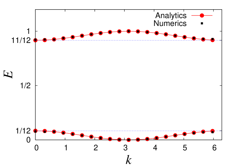
Figure 1: Numerically obtained eigenvalues of the Floquet operator as compared with the analytical expressions in Eqs. (44-45), for $V=1,~{}T=0.5$, and $\gamma=1$. All other eigenvalues are zero. We have two particles on 20 sites.

In Figs. 2-3, we show the time evolution of two particles placed on a ring of 20 sites, with various initial conditions, interaction strengths and kicking; this system has 190 states. The time evolution is found by numerically evaluating the Floquet operator $U$ given in Eq. (6); we have taken $\gamma=1$ and $T=0.5$ in all these studies. We discuss below our numerical results and how they compare with what we expect from the effective Hamiltonian up to order $\gamma^{2}T^{2}V$ that we have derived above.

In Fig. 2, we consider the time evolution when the initial state has the two particles on adjacent sites. The first two rows of this figure show that the particles spread out over the ring if there is no kicking; there is no major difference between the interacting and non-interacting cases. The third row shows that the particles are dynamically localized if there is kicking but no interaction. The fourth row shows that there is no dynamical localization if there is both kicking and interaction; however, since $\gamma T=0.5$ is small, the two particle bound state dispersion is almost flat which implies that the group velocity is small. Hence the particles spread out over the ring more slowly compared to the first two rows where there is no kicking. (In the fourth row, the eigenstates have large components on states of the form $|j,j+1\rangle$).

In Figs. 3, we show the time evolution of two particles on 20 sites in the presence of kicking. In Figs. 3 (i)-(ii), the initial state has two particles which are separated by two lattice spacings. Figure (i) shows dynamical localization in the absence of interactions ($V=0$). The behavior in Fig. 3 (ii) (where interactions are present with $V=1$) is similar to that in Fig. 2 (iv), except that the eigenstates now have large components on states of the form $|j,j+2\rangle$. In Figs. 3 (iii) and (iv), the initial state has two particles which are separated by three and four lattice spacings, namely, states of the form $|j,j+3\rangle$ and $|j,j+4\rangle$ respectively. In these cases, the states has no overlap with the two-particle bound states and therefore do not disperse. In the presence of interactions the particles seem to be localized. Looking more closely, we find that the particles do spread a little bit when they are initially separated by three lattice spacings but not for four lattice spacings. This occurs because the wave function in the case of three lattice spacings has a small overlap with the two-particle bound states when we go to terms in the effective Hamiltonian which are of higher order than $\gamma^{2}T^{2}V$.

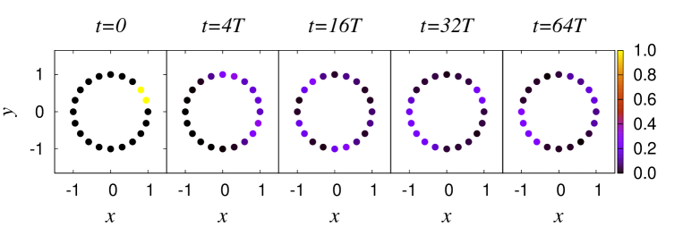
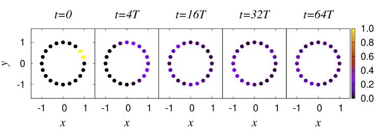
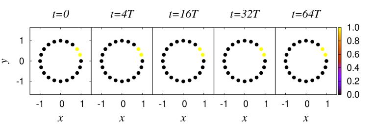
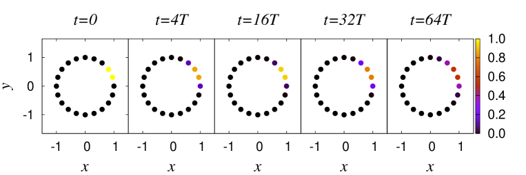
Figure 2: Time evolution of a two-particle state for four cases: (i) $V=0$, no kicking, (ii) $V=1$, no kicking, (iii) $V=0$, with kicking, and (iv) $V=1$, with kicking. In all cases $\gamma=1$ and $T=0.5$. There are two particles on $20$ sites, and they are initially located at two adjacent sites. The color shows the expectation value of the particle number at different sites.

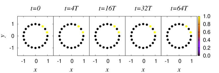
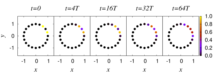
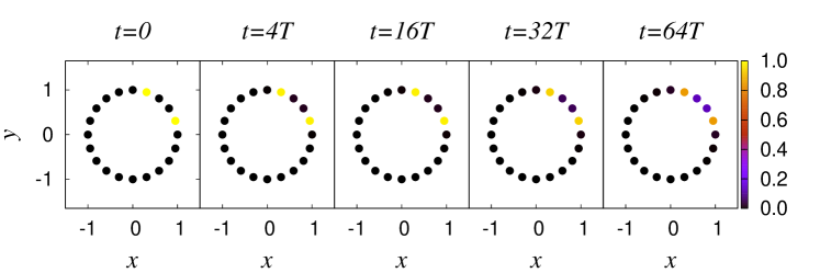
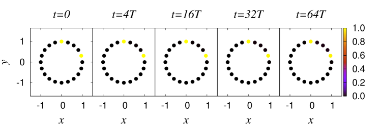
Figure 3: Time evolution of a state with two particles on 20 sites in the presence of kicking, for four cases. In (i) the two particles are initially on adjacent sites and there is no interaction ($V=0$). The state is dynamically localized due to kicking. In (ii)-(iv) the initial distance between the particles is progressively increased from two to four lattice spacings, and interactions are present with $V=1$. The color shows the expectation value of the particle number at different sites. Note that with increasing initial spacing the overlap with the two-particle bound states gets reduced, and the states get more localized.

IV.2 States with three or more particles

We will now study what happens when there are more than two particles. We begin with the case of three particles. Assuming that they are on three neighboring sites, Table III shows the action of the different terms in Eq. (33) on the state $|j,j+1,j+2\rangle$.

Terms in $H_{eff}$	Acting on $|j,j+1,j+2\rangle$
$Vn_{j}n_{j+1}$	$2V|j,j+1,j+2\rangle$
$-\frac{i\gamma TV}{2}(c^{\dagger}_{j+1}c_{j}-c_{j}^{\dagger}c_{j+1})(n_{j-1}-n_{j+2})$	$-\frac{i\gamma TV}{2}(|j-1,j+1,j+2\rangle$
	$+|j,j+1,j+3\rangle)$
$-\frac{\gamma^{2}T^{2}V}{3}(n_{j}-n_{j+1})(n_{j-1}-n_{j+2})$	$-\frac{2\gamma^{2}T^{2}V}{3}|j,j+1,j+2\rangle$
$-\frac{\gamma^{2}T^{2}V}{6}(c^{\dagger}_{j-1}c_{j+1}+c^{\dagger}_{j+1}c_{j-1})(n_{j+2}+n_{j-2}-2n_{j})$	$-$
$-\frac{\gamma^{2}T^{2}V}{3}(c^{\dagger}_{j-1}c_{j-2}-c^{\dagger}_{j-2}c_{j-1})(c^{\dagger}_{j}c_{j+1}-c^{\dagger}_{j+1}c_{j})$

Table 3: Effect of various terms in $H_{eff}$ acting on the state $|j,j+1,j+2\rangle$. The $-$ symbol in the right column means we have states which only contribute to the bound state at orders higher than $\gamma^{2}T^{2}V$.

A second order process involving the second term in $H_{eff}$ brings an initial state $|j,j+1,j+2\rangle$ back to itself, with an amplitude $\frac{\gamma^{2}T^{2}V^{2}}{4(2V-V)}=\gamma^{2}T^{2}V/4$; the denominator $2V-V$ is the difference in the unperturbed energies of the initial state and the intermediate states given by $|j-1,j+1,j+2\rangle$ and $|j,j+1,j+3\rangle$. This process can happen in two ways since there are two possible intermediate states; hence this contribution is equal to $\gamma^{2}T^{2}V/2$. The total contribution is therefore, $(\frac{1}{2}-\frac{2}{3})\gamma^{2}T^{2}V=-\gamma^{2}T^{2}V/6$. Therefore, we find non-dispersing eigenstates with quasienergy $2V-(\gamma^{2}T^{2}V/6)$. The number of such states is equal to the number of sites $N$, since the index $j$ of the first particle can take any value from 1 to $N$.

In fact, there is an interesting solution for any number of particles $n$, where $N-2>n>2$. Consider a state where $n$ particles are located next to each other. Due to the second order process described above, this is an eigenstate of $H_{eff}$ with quasienergy

$$E_{n}~{}=~{}(n-1)V~{}-~{}\frac{\gamma^{2}T^{2}V}{6}.$$ (46)

Thus we have non-dispersing states of clustered particles; the number of such states is $N$. These multi-particle states are dynamically localized due to the kicking, and this remains true even when interactions are taken into account. The flat dispersion for these states is shown in Fig. 4 for some representative cases; we find that the eigenvalues of the Floquet operator obtained numerically agree very well with the analytical expression.

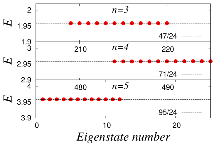
Figure 4: Numerically obtained eigenvalues of the Floquet operator as compared with the analytical expression in Eq. (46), for $V=1,~{}T=0.5$ and $\gamma=1$, for $n=3,~{}4,~{}5$ particles on $12$ sites. Note that for each $n$ we have $N=12$ eigenvalues which are non-dispersing.

As a striking demonstration of the dynamical localization of multi-particle systems, we show the time evolution of a system with four particles on 12 sites in Fig. 5. We see that the particles remain dynamically localized when they are initially located on four adjacent sites.

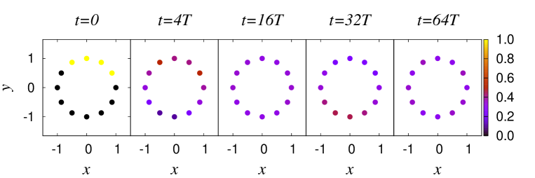
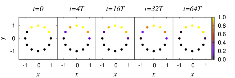
Figure 5: Time evolution of a four-particle state: (i) $V=1$, no kicking, (ii) $V=1$, with kicking. In both cases $\gamma=1$ and $T=0.5$. There are four particles on 12 sites, and they are initially located on four adjacent sites. The second row shows that the particles do not move even in the presence of interactions.

V Spin-$1/2$ fermions with on-site interactions

We now look at the one-dimensional model of spin-1/2 interactions with on-site interactions between spin-up and spin-down electrons. This is called the Hubbard model and it is also exactly solvable by the Bethe ansatz mattis93 ; sutherland04 . The Hamiltonian of the model is

$$H~{}=-\gamma~{}\sum_{j,\sigma}(c_{j\sigma}^{\dagger}c_{j+1~{}\sigma}+H.c.)~{}+~{}U~{}\sum_{j}~{}n_{j\uparrow}n_{j\downarrow}.$$ (47)

We naturally identify the first term as $H_{NI}$ and the second term as $H_{I}$. As before, we first evaluate $[H_{NI},H_{I}]$ which has relevant terms,

$$= [c_{j\sigma}^{\dagger}c_{j+1~{}\sigma}+c^{\dagger}_{j+1~{}\sigma}c_{j\sigma},n_{j\uparrow}n_{j\downarrow}+n_{j+1~{}\uparrow}n_{j+1~{}\downarrow}]$$

$$= (c^{\dagger}_{j+1~{}\uparrow}c_{j\uparrow}-c_{j\uparrow}^{\dagger}c_{j+1~{}\uparrow})(n_{j\downarrow}-n_{j+1~{}\downarrow})+(c^{\dagger}_{j+1~{}\downarrow}c_{j\downarrow}-c_{j\downarrow}^{\dagger}c_{j+1~{}\downarrow})(n_{j\uparrow}-n_{j+1~{}\uparrow}).$$

Next we find

$$[H_{NI},[H_{NI},H_{I}]]~{}=~{}\gamma^{2}T^{2}U$$ (49)

$$\times \Big{[}4~{}\Big{(}(n_{j\uparrow}-n_{j+1~{}\uparrow})(n_{j\downarrow}-n_{j+1~{}\downarrow})+(c^{\dagger}_{j\uparrow}c_{j+1~{}\uparrow}-c^{\dagger}_{j+1~{}\uparrow}c_{j\uparrow})(c^{\dagger}_{j\downarrow}c_{j+1~{}\downarrow}-c^{\dagger}_{j+1~{}\downarrow}c_{j\downarrow})\Big{)}$$

$$~{}+\Big{(}\big{(}(c^{\dagger}_{j\uparrow}c_{j+2~{}\uparrow}+c^{\dagger}_{j+2~{}\uparrow}c_{j\uparrow})(n_{j\downarrow}-n_{j+1~{}\downarrow})$$

$$~{}~{}~{}~{}~{}~{}~{}+(c^{\dagger}_{j\uparrow}c_{j+1~{}\uparrow}-c^{\dagger}_{j+1~{}\uparrow}c_{j\uparrow})(c^{\dagger}_{j+2~{}\downarrow}c_{j+1~{}\downarrow}-c^{\dagger}_{j+1~{}\downarrow}c_{j+2~{}\downarrow})\big{)}+\big{(}\uparrow\leftrightarrow\downarrow\big{)}\Big{)}$$

$$~{}+\Big{(}\big{(}(c^{\dagger}_{j+1~{}\uparrow}c_{j-1~{}\uparrow}+c^{\dagger}_{j-1~{}\uparrow}c_{j+1~{}\uparrow})(-n_{j\downarrow}+n_{j+1~{}\downarrow})$$

$$~{}~{}~{}~{}~{}~{}~{}+(c^{\dagger}_{j\uparrow}c_{j+1~{}\uparrow}-c^{\dagger}_{j+1~{}\uparrow}c_{j\uparrow})(c^{\dagger}_{j\downarrow}c_{j-1~{}\downarrow}-c^{\dagger}_{j-1~{}\downarrow}c_{j\downarrow})\big{)}+\big{(}\uparrow\leftrightarrow\downarrow\big{)}\Big{)}\Big{]}.$$

The effective Hamiltonian in (20) therefore takes the form

$$H_{eff} = U~{}\sum_{j}~{}n_{j\uparrow}n_{j\downarrow}$$

$$-\frac{i\gamma TU}{2}\sum_{j,\sigma}(c^{\dagger}_{j+1~{}\sigma}c_{j\sigma}-c_{j\sigma}^{\dagger}c_{j+1~{}\sigma})(n_{j\bar{\sigma}}-n_{j+1~{}\bar{\sigma}})$$

$$-\frac{\gamma^{2}T^{2}U}{6}\sum_{j}\Big{[}4\big{(}(n_{j\uparrow}-n_{j+1~{}\uparrow})(n_{j\downarrow}-n_{j+1~{}\downarrow})$$

$$~{}~{}~{}~{}~{}~{}~{}~{}~{}~{}~{}~{}~{}~{}~{}~{}~{}+(c^{\dagger}_{j\uparrow}c_{j+1~{}\uparrow}-c^{\dagger}_{j+1~{}\uparrow}c_{j\uparrow})(c^{\dagger}_{j\downarrow}c_{j+1~{}\downarrow}-c^{\dagger}_{j+1~{}\downarrow}c_{j\downarrow})\big{)}$$

$$~{}~{}~{}~{}~{}~{}~{}~{}~{}~{}~{}~{}~{}~{}~{}~{}~{}+\left((c^{\dagger}_{j\uparrow}c_{j+2~{}\uparrow}+c^{\dagger}_{j+2~{}\uparrow}c_{j\uparrow})(n_{j\downarrow}-n_{j+1~{}\downarrow})+(\uparrow\leftrightarrow\downarrow)\right)$$

$$~{}~{}~{}~{}~{}~{}~{}~{}~{}~{}~{}~{}~{}~{}~{}~{}~{}-\left((c^{\dagger}_{j-1~{}\uparrow}c_{j+1~{}\uparrow}+c^{\dagger}_{j+1~{}\uparrow}c_{j-1~{}\uparrow})(n_{j\downarrow}-n_{j+1~{}\downarrow})+(\uparrow\leftrightarrow\downarrow)\right)$$

$$~{}~{}~{}~{}~{}~{}~{}~{}~{}~{}~{}~{}~{}~{}~{}~{}~{}+\Big{(}2(c^{\dagger}_{j\uparrow}c_{j+1~{}\uparrow}-c^{\dagger}_{j+1~{}\uparrow}c_{j\uparrow})(c^{\dagger}_{j+2~{}\downarrow}c_{j+1~{}\downarrow}-c^{\dagger}_{j+1~{}\downarrow}c_{j+2~{}\downarrow})+(\uparrow\leftrightarrow\downarrow)\Big{)}\Big{]}.$$

We now use the effective Hamiltonian in Eq. (LABEL:eq:effHspin) to look at two-particle states. In particular, we will again search for bound states. In the Hubbard model, two particles can interact with each other only if they have opposite spins. We will therefore take the two particles to have spins $\uparrow$ and $\downarrow$.

We first look at a state where the two particles are at the same site $j$. (This is a spin singlet state). A momentum eigenstate will be of the form

$$|\psi_{k}\rangle~{}=~{}\sum_{j}~{}e^{ikj}|j\uparrow,j\downarrow\rangle.$$ (51)

(For $k=\pi$, this is again an exact eigenstate of both the Hamiltonian in Eq. (47) and of the kicking problem since $N_{A}=0$ or 2 implies that $U_{K}|\psi_{k}\rangle=|\psi_{k}\rangle$). We will look at the effect of each of the terms in Eq. (LABEL:eq:effHspin) on the state $|j\uparrow,j\downarrow\rangle$. This is shown in Table IV, with a sum over $j$ being assumed.

Terms in $H_{eff}$	Acting on $e^{ikj}|j\uparrow,j\downarrow\rangle$
$Un_{j\uparrow}n_{j\downarrow}$	$Ue^{ikj}|j\uparrow,j\downarrow\rangle$
$-\frac{i\gamma TU}{2}(c^{\dagger}_{j+1~{}\sigma}c_{j\sigma}-c_{j\sigma}^{\dagger}c_{j+1~{}\sigma})(n_{j\bar{\sigma}}-n_{j+1~{}\bar{\sigma}})$	$-\frac{i\gamma TU}{2}e^{ikj}(|j\uparrow,j+1~{}\downarrow\rangle+|j\uparrow,j-1~{}\downarrow\rangle$
	$+|j+1~{}\uparrow,j\downarrow\rangle+|j-1~{}\uparrow,j\downarrow\rangle)$
$-\frac{\gamma^{2}T^{2}U}{6}\Big{[}4\big{(}(n_{j\uparrow}-n_{j+1~{}\uparrow})(n_{j\downarrow}-n_{j+1~{}\downarrow})$	$-\frac{2\gamma^{2}T^{2}U}{3}e^{ikj}(2|j\uparrow,j\downarrow\rangle$
$+(c^{\dagger}_{j\uparrow}c_{j+1~{}\uparrow}-c^{\dagger}_{j+1~{}\uparrow}c_{j\uparrow})(c^{\dagger}_{j\downarrow}c_{j+1~{}\downarrow}-c^{\dagger}_{j+1~{}\downarrow}c_{j\downarrow})\big{)}$	$+|j+1~{}\uparrow,j+1~{}\downarrow\rangle+|j-1~{}\uparrow,j-1~{}\downarrow\rangle)$
$+\left((c^{\dagger}_{j\uparrow}c_{j+2~{}\uparrow}+c^{\dagger}_{j+2~{}\uparrow}c_{j\uparrow})(n_{j\downarrow}-n_{j+1~{}\downarrow})+(\uparrow\leftrightarrow\downarrow)\right)$	$-$
$-\left((c^{\dagger}_{j-1~{}\uparrow}c_{j+1~{}\uparrow}+c^{\dagger}_{j+1~{}\uparrow}c_{j-1~{}\uparrow})(n_{j\downarrow}-n_{j+1~{}\downarrow})+(\uparrow\leftrightarrow\downarrow)\right)$
$+\Big{(}2(c^{\dagger}_{j\uparrow}c_{j+1~{}\uparrow}-c^{\dagger}_{j+1~{}\uparrow}c_{j\uparrow})(c^{\dagger}_{j+2~{}\downarrow}c_{j+1~{}\downarrow}-c^{\dagger}_{j+1~{}\downarrow}c_{j+2~{}\downarrow})$
$+(\uparrow\leftrightarrow\downarrow)\Big{)}\Big{]}$

Table 4: Effect of various terms in $H_{eff}$ on the state $e^{ikj}|j\uparrow,j\downarrow\rangle$. The $-$ symbol in the right column means we have states which only contribute to the bound state at orders higher than $\gamma^{2}T^{2}U$.

From Table IV, we see that the terms of order $\gamma TU$ can give rise to a second order process where an initial state $|j\uparrow,j\downarrow\rangle$ can go to intermediate states $|j\uparrow,j\pm 1~{}\downarrow\rangle$ and then return to $|j\uparrow,j\downarrow\rangle$. The contribution of this is

$$\frac{\gamma^{2}T^{2}U^{2}}{4}~{}2e^{ikj}(1+e^{ik})(1+e^{-ik})~{}|j\uparrow,j\downarrow\rangle$$ (52)

divided by the energy difference between the initial and intermediate states which is $U$. We therefore get

$$\gamma^{2}T^{2}U(1+\cos k).$$ (53)

To this we add the contribution of the terms of order $\gamma^{2}T^{2}U$ which is equal to

$$-\frac{4\gamma^{2}T^{2}U}{3}(1+\cos k).$$ (54)

The total quasienergy is therefore

$$E_{1k} = U~{}+~{}\gamma^{2}T^{2}U~{}(1-\frac{4}{3})~{}(1+\cos k)$$ (55)

$$= U~{}-~{}\frac{2\gamma^{2}T^{2}U}{3}~{}\cos^{2}\left(\frac{k}{2}\right).$$

This is the quasienergy for a wave function in which there is a large amplitude for the particles with up and down spins to be at the same site.

We now look at a different case where the two particles with opposite spins (to be denoted as $\sigma$ and $\bar{\sigma}$) are at adjacent sites $j$ and $j+1$. The wave function with momentum $k$ is then

$$|\psi_{k}\rangle~{}=~{}\sum_{j\sigma}e^{ik(j+1/2)}s_{\sigma}|j\sigma,j+1~{}\bar{\sigma}\rangle,$$ (56)

where $s_{\sigma}=+1$ if $\sigma=\uparrow$ and $-1$ if $\sigma=\downarrow$. (This is again a spin singlet state). The action of the different terms in Eq. (LABEL:eq:effHspin) on the wave function in Eq. (56) is shown in Table V, with a sum over $j$ and $\sigma$ being assumed.

Terms in $H_{eff}$	Acting on $e^{ik(j+1/2)}s_{\sigma}|j\sigma,j+1~{}\bar{\sigma}\rangle$
$Un_{j\uparrow}n_{j\downarrow}$	$zero$
$-\frac{i\gamma TU}{2}(c^{\dagger}_{j+1~{}\sigma}c_{j\sigma}-c_{j\sigma}^{\dagger}c_{j+1~{}\sigma})(n_{j\bar{\sigma}}-n_{j+1~{}\bar{\sigma}})$	$i\gamma TUe^{ik(j+1/2)}(|j\uparrow,j\downarrow\rangle$
	$+|j+1~{}\uparrow,j+1~{}\downarrow\rangle)$
$-\frac{\gamma^{2}T^{2}U}{6}\Big{[}4\big{(}(n_{j\uparrow}-n_{j+1~{}\uparrow})(n_{j\downarrow}-n_{j+1~{}\downarrow})$	$\frac{4\gamma^{2}T^{2}U}{3}e^{ik(j+1/2)}s_{\sigma}|j\sigma,j+1~{}\bar{\sigma}\rangle$
$+(c^{\dagger}_{j\uparrow}c_{j+1~{}\uparrow}-c^{\dagger}_{j+1~{}\uparrow}c_{j\uparrow})(c^{\dagger}_{j\downarrow}c_{j+1~{}\downarrow}-c^{\dagger}_{j+1~{}\downarrow}c_{j\downarrow})\big{)}$
$+\left((c^{\dagger}_{j\uparrow}c_{j+2~{}\uparrow}+c^{\dagger}_{j+2~{}\uparrow}c_{j\uparrow})(n_{j\downarrow}-n_{j+1~{}\downarrow})+(\uparrow\leftrightarrow\downarrow)\right)$	$\frac{2\gamma^{2}T^{2}U}{3}e^{ik(j+1/2)}s_{\sigma}~{}\times$
$-\left((c^{\dagger}_{j-1~{}\uparrow}c_{j+1~{}\uparrow}+c^{\dagger}_{j+1~{}\uparrow}c_{j-1~{}\uparrow})(n_{j\downarrow}-n_{j+1~{}\downarrow})+(\uparrow\leftrightarrow\downarrow)\right)$	$(|j+1~{}\sigma,j+2~{}\bar{\sigma}\rangle+|j-1~{}\sigma,j\bar{\sigma}\rangle)$
$+\Big{(}2(c^{\dagger}_{j\uparrow}c_{j+1~{}\uparrow}-c^{\dagger}_{j+1~{}\uparrow}c_{j\uparrow})(c^{\dagger}_{j+2~{}\downarrow}c_{j+1~{}\downarrow}-c^{\dagger}_{j+1~{}\downarrow}c_{j+2~{}\downarrow})$
$+(\uparrow\leftrightarrow\downarrow)\Big{)}\Big{]}$

Table 5: Effect of various terms in $H_{eff}$ on the state $e^{ik(j+1/2)}s_{\sigma}|j\sigma,j+1~{}\bar{\sigma}\rangle$.

Table V shows that the term of order $\gamma TU$ takes an initial state $s_{\sigma}|j\sigma,j+1\bar{\sigma}\rangle$ to an intermediate state $|j\sigma,j\bar{\sigma}\rangle$ and then back to the initial state. This gives a contribution equal to

$$\frac{\gamma^{2}T^{2}U^{2}}{4}~{}2e^{ik(j+1/2)}(1+e^{ik})(1+e^{-ik})s_{\sigma}|j\sigma,j+1~{}\bar{\sigma}\rangle.$$ (57)

Dividing by a denominator $-U$ equal to the energy difference of the two states, we get

$$-\gamma^{2}T^{2}U~{}(1+\cos k).$$ (58)

Adding the contribution from the terms of order $\gamma^{2}T^{2}U$, we get a total contribution equal to

$$E_{2k} = (\frac{4}{3}-1)\gamma^{2}T^{2}U~{}(1+\cos k)$$ (59)

$$= \frac{2\gamma^{2}T^{2}U}{3}~{}\cos^{2}\left(\frac{k}{2}\right).$$

In Fig. 6 we compare the numerically obtained eigenvalues of the Floquet operator for two particles with spins $\uparrow$ and $\downarrow$ with the analytical expressions in Eqs. (55) and (59). The agreement can be seen to be excellent.

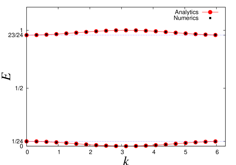
Figure 6: Numerically obtained eigenvalues of the effective Hamiltonian as compared with the analytical expressions in Eqs. (55) and (59), for $U=1,~{}T=0.25$ and $\gamma=1$. All other eigenvalues are zero. We have one $\uparrow$ and one $\downarrow$ particle on $20$ sites.

In Fig. 7, we show the time evolution of a system with two particles, with spins $\uparrow$ and $\downarrow$, on 20 sites; the particles are initially at the same site. The third row shows that the particles are dynamically localized when there is kicking but no interactions. The fourth row shows that when interactions are turned on, the particles move but very slowly; this is because the group velocity for the dispersion in Eq. (55) is small when $\gamma^{2}T^{2}$ is small.

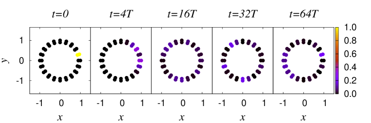
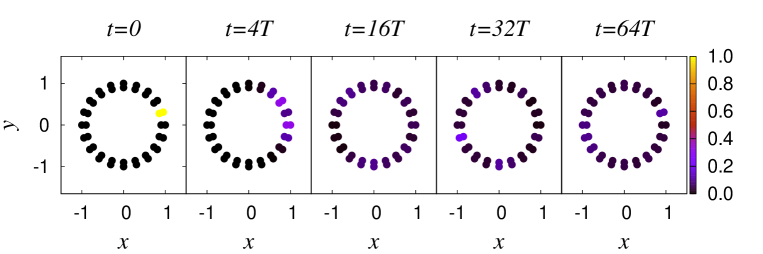
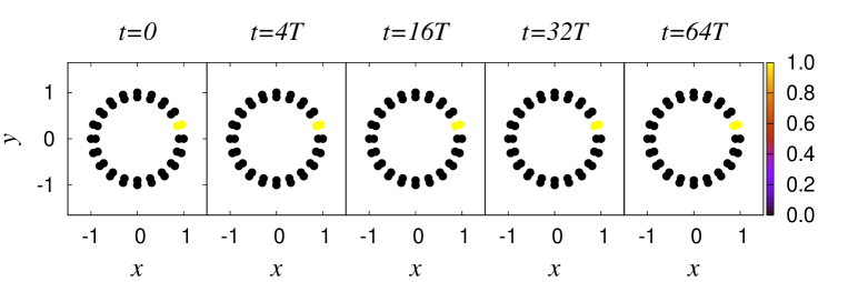
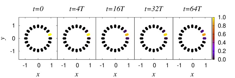
Figure 7: Time evolution of a two-particle state for four cases: (i) $U=0$, no kicking, (ii) $U=1$, no kicking, (iii) $U=0$, with kicking, (iv) $U=1$, with kicking. In all cases $\gamma=1$ and $T=0.25$. There are two particles, with spins $\uparrow$ and $\downarrow$, on 20 sites, and they are initially located at the same site. The colors of the dots on the outer (inner) ring show the expectation values of the number of up (down) spin particles at different sites.

VI Bosons with on-site interactions

As our final example of an interacting system, we will consider a system of bosons with on-site interactions in one dimension. This is called the Bose Hubbard model. For a system with $N$ sites and periodic boundary conditions, the Hamiltonian is

$$H~{}=~{}\sum_{j=1}^{N}~{}[-\gamma(b_{j}^{\dagger}b_{j+1}+H.c.)~{}+~{}\frac{U}{2}n_{j}(n_{j}-1)],$$ (60)

where $n_{j}=b_{j}^{\dagger}b_{j}$ is the particle number at site $j$.

As before we first evaluate

$$[H_{NI},H_{I}] = -\gamma U\left((b^{\dagger}_{j+1}n_{j}b_{j}-b^{\dagger}_{j}n_{j}b_{j+1})-(b^{\dagger}_{j+1}n_{j+1}b_{j}-b^{\dagger}_{j}n_{j+1}b_{j+1})\right)$$ (61)

$$= -\gamma U\left(b^{\dagger}_{j+1}(n_{j}-n_{j+1})b_{j}-b^{\dagger}_{j}(n_{j}-n_{j+1})b_{j+1}\right).$$

The next term is

$$[H_{NI},[H_{NI},H_{I}]] = \gamma^{2}T^{2}U\Big{[}2\Big{(}n_{j}(n_{j}-1)+n_{j+1}(n_{j+1}-1)-4n_{j}n_{j+1}\Big{)}$$ (62)

$$+2\Big{(}b^{\dagger}_{j}b_{j+1}b^{\dagger}_{j}b_{j+1}+H.c.\Big{)}$$

$$+\Big{(}b^{\dagger}_{j}(n_{j}-2n_{j+1})b_{j+2}+H.c.\Big{)}+\Big{(}b^{\dagger}_{j}b_{j+1}b^{\dagger}_{j+2}b_{j+1}+H.c.\Big{)}$$

$$+\Big{(}b^{\dagger}_{j-1}(n_{j+1}-2n_{j})b_{j+1}+H.c.\Big{)}+\Big{(}b^{\dagger}_{j-1}b_{j}b^{\dagger}_{j+1}b_{j}+H.c.\Big{)}\Big{]}.$$

Putting all this together, the effective Hamiltonian in Eq. (20) takes the form

$$H_{eff} = \frac{U}{2}~{}\sum_{j}~{}n_{j}(n_{j}-1)$$ (63)

$$- \frac{i\gamma TU}{2}~{}\sum_{j}~{}\left(b^{\dagger}_{j+1}(n_{j}-n_{j+1})b_{j}-b^{\dagger}_{j}(n_{j}-n_{j+1})b_{j+1}\right)$$ (64)

$$- \frac{\gamma^{2}T^{2}U}{3}~{}\sum_{j}~{}\Big{[}2n_{j}(n_{j}-1)-4n_{j}n_{j+1}$$ (65)

$$+ \Big{(}b^{\dagger}_{j}b_{j+1}(b^{\dagger}_{j}+b^{\dagger}_{j+2})b_{j+1}+H.c.\Big{)}~{}+~{}\frac{1}{2}\Big{(}b^{\dagger}_{j}(n_{j+2}+n_{j}-4n_{j+1})b_{j+2}+H.c.\Big{)}\Big{]}.$$ (66)

We can again look for two-particle bound states just as in the previous sections. We first look for a state with momentum $k$ which consists mainly of states in which both the particles are at site $j$, namely,

$$|\psi_{1k}\rangle~{}=~{}\sum_{j}~{}e^{ikj}|j,j\rangle.$$ (67)

(For $k=\pi$, this is an exact eigenstate of the Hamiltonian in Eq. (60)) and of the kicking problem since $U_{K}|\psi_{1k}\rangle=|\psi_{1k}\rangle$. The action of $H_{eff}$ on the state in (67) is given in Table VI.

Terms in $H_{eff}$	Acting on $e^{ikj}|j,j\rangle$
$\frac{U}{2}~{}n_{j}(n_{j}-1)$	$Ue^{ikj}|j,j\rangle$
$-\frac{i\gamma TU}{2}~{}\left(b^{\dagger}_{j+1}(n_{j}-n_{j+1})b_{j}-b^{\dagger}_{j}(n_{j}-n_{j+1})b_{j+1}\right)$	$-\frac{i\gamma TU}{2}\sqrt{2}e^{ikj}\left(|j,j+1\rangle+|j-1,j\rangle\right)$
$-\frac{\gamma^{2}T^{2}U}{3}~{}\Big{[}2n_{j}(n_{j}-1)-4n_{j}n_{j+1}$	$-\frac{4\gamma^{2}T^{2}U}{3}e^{ikj}|j,j\rangle$
$+\Big{(}b^{\dagger}_{j}b_{j+1}(b^{\dagger}_{j}+b^{\dagger}_{j+2})b_{j+1}+H.c.\Big{)}$	$-\frac{2\gamma^{2}T^{2}U}{3}e^{ikj}(|j-1,j-1\rangle+|j+1,j+1\rangle)$
$+~{}\frac{1}{2}\Big{(}b^{\dagger}_{j}(n_{j+2}+n_{j}-4n_{j+1})b_{j+2}+H.c.\Big{)}\Big{]}$	$-$

Table 6: Effect of various terms in $H_{eff}$ on the state $e^{ikj}|j,j\rangle$.

The terms in the second line in Table VI take $|j,j\rangle$ to an intermediate state $|j,j\pm 1\rangle$ and act again to take it back to $|j,j\rangle$ with a contribution

$$\frac{\gamma^{2}T^{2}U^{2}}{4}~{}2e^{ikj}(1+e^{ik})(1+e^{-ik})|j,j\rangle.$$ (68)

Dividing by the energy difference between the initial and intermediate states, $U$, gives the contribution

$$\gamma^{2}T^{2}U(1+\cos k).$$ (69)

The third and fourth lines in Table VI give a diagonal contribution of the form

$$-~{}\frac{4\gamma^{2}T^{2}U}{3}~{}(1+\cos k).$$ (70)

The total contribution to the quasienergy is therefore

$$E_{1k} = U~{}+~{}\gamma^{2}T^{2}U~{}(1-\frac{4}{3})~{}(1+\cos k)$$ (71)

$$= U~{}-~{}\frac{2\gamma^{2}T^{2}U}{3}~{}\cos^{2}\left(\frac{k}{2}\right).$$

We now look at the second kind of two-particle bound states which consists mainly of states where the particles are on sites $j$ and $j+1$, namely,

$$|\psi_{2k}\rangle~{}=~{}\sum_{j}~{}e^{ik(j+1/2)}~{}|j,j+1\rangle.$$ (72)

The action of $H_{eff}$ on this state is given in Table VII.

Terms in $H_{eff}$	Acting on $e^{ik(j+1/2)}|j,j+1\rangle$
$\frac{U}{2}~{}n_{j}(n_{j}-1)$	$zero$
$-\frac{i\gamma TU}{2}~{}\left(b^{\dagger}_{j+1}(n_{j}-n_{j+1})b_{j}-b^{\dagger}_{j}(n_{j}-n_{j+1})b_{j+1}\right)$	$\frac{i\gamma TU}{2}\sqrt{2}e^{ik(j+1/2)}\left(|j,j\rangle+|j+1,j+1\rangle\right)$
$-\frac{\gamma^{2}T^{2}U}{3}~{}\Big{[}2n_{j}(n_{j}-1)-4n_{j}n_{j+1}$	$\frac{4\gamma^{2}T^{2}U}{3}e^{ik(j+1/2)}|j,j+1\rangle$
$+\Big{(}b^{\dagger}_{j}b_{j+1}(b^{\dagger}_{j}+b^{\dagger}_{j+2})b_{j+1}+H.c.\Big{)}$	$-$
$+~{}\frac{1}{2}\Big{(}b^{\dagger}_{j}(n_{j+2}+n_{j}-4n_{j+1})b_{j+2}+H.c.\Big{)}\Big{]}$	$\frac{2\gamma^{2}T^{2}U}{3}e^{ik(j+1/2)}(|j-1,j\rangle+|j+1,j+2\rangle)$

Table 7: Effects of various terms in $H_{eff}$ on the state $e^{ik(j+1/2)}|j,j+1\rangle$.

The second line in Table VII takes $|j,j+1\rangle$ to intermediate states $|j,j\rangle$ and $|j+1,j+1\rangle$, and acts again to take it back to $|j,j+1\rangle$ with a contribution

$$\frac{\gamma^{2}T^{2}U^{2}}{4}~{}2e^{ikj}(1+e^{ik})(1+e^{-ik})|j,j+1\rangle.$$ (73)

Dividing by the energy difference between the initial and intermediate states, $-U$, gives the contribution

$$-\gamma^{2}T^{2}U(1+\cos k).$$ (74)

To this we have to add the contributions from the third and fifth lines of Table VII. The total quasienergy is therefore

$$E_{2k} = \gamma^{2}T^{2}U~{}(\frac{4}{3}-1)~{}(1+\cos k)$$ (75)

$$= \frac{2\gamma^{2}T^{2}U}{3}~{}\cos^{2}\left(\frac{k}{2}\right).$$

We note that the dispersions given in Eqs. (71) and (75) are identical to Eqs. (55) and (59). A comparison between the numerically obtained eigenvalues of the effective Hamiltonian and the analytical expressions in Eqs. (71) and (75) therefore looks exactly the same as in Fig. 6 if we take the same values of $U,~{}T$ and $\gamma$.

Finally, we find that just as in the case of spinless fermions, we have $n$-particle bound states which are dynamically localized and which do not disperse if $n\geq 3$; such bound states consist mainly of states in which all the $n$ particles are on the same site $j$. For a system of $N$ sites, there are $N$ such bound states corresponding to the different possible values of $j$. The quasienergy of these states is given by

$$E_{n}~{}=~{}\frac{U}{2}n(n-1)~{}\left(1~{}-~{}\frac{\gamma^{2}T^{2}}{3}\right).$$ (76)

We have verified that our numerical results for $n$-particle states match this analytical expression.

VI.1 Effective Hamiltonian when each site has a double degeneracy

We will now consider what happens if a uniform potential is applied at all sites (this is equivalent to applying a chemical potential $\mu$) in such a way that, in the absence of periodic driving, the ground state of the interaction part of the Hamiltonian has a two-fold degeneracy at each site corresponding to occupancies $p$ and $p+1$; here $p$ can be $0,1,2,\cdots$. (These are the points where the Mott lobes meet in the phase diagram of the Bose Hubbard model in the limit of zero hopping freericks94 ). Namely, we modify the interaction term in Eq. (60) to

$$\frac{U}{2}(n_{j}-c)^{2},~{}~{}{\rm where}~{}~{}c~{}=~{}p~{}+~{}\frac{1}{2},$$ (77)

so that the states with $n_{j}=p$ and $p+1$ are degenerate with energy $U/8$. We then find that the effective Hamiltonian is given by Eqs. (63-66) except that Eq. 63 is now replaced by $\frac{U}{2}~{}\sum_{j}~{}(n_{j}-p-\frac{1}{2})^{2}$.

We will now assume $U$ is so large that the energies of the states with $n_{j}=p$ and $p+1$ are well separated from the energies of states with any other value of $n_{j}$. With this assumption, we will turn on the periodic driving and derive an effective Hamiltonian $H_{eff}$ in the space of states in which $n_{j}=p$ or $p+1$ at each site. To this end, we introduce pseudo-spin Pauli matrices $\sigma^{a}_{j}$ at each site (where $a=x,y,z$), so that the states with $n_{j}=p$ and $p+1$ correspond to $\sigma^{z}_{j}=-1$ and $+1$ respectively. Hence

$$n_{j}~{}=~{}p~{}+~{}\frac{1+\sigma^{z}_{j}}{2}.$$ (78)

Further, within the space of these two states, we have the identities

$$b_{j}^{\dagger}~{}=~{}\sqrt{p+1}~{}\sigma_{j}^{+}~{}~{}~{}~{}{\rm and}~{}~{}~{}~{}b_{j}~{}=~{}\sqrt{p+1}~{}\sigma_{j}^{-}.$$ (79)

We will derive $H_{eff}$ up to order $\gamma^{2}T^{2}U$. As before there are two kinds of contributions: those coming from second order processes induced by the terms of order $\gamma TU$ in Eq. (64), and those coming directly from the terms of order $\gamma^{2}T^{2}U$ in Eqs. (65-66). The second order processes can lead to terms in $H_{eff}$ which involve either two sites or three sites. We present the details of the calculation in Appendix B. The effective Hamiltonian is found to be

$$H_{eff} = \frac{\gamma^{2}T^{2}U}{12}~{}\sum_{j}~{}\Big{[}2(p+1)\sigma^{z}_{j}~{}+~{}\sigma^{z}_{j}\sigma^{z}_{j+1}~{}+~{}(p+1)(p+1+\sigma^{z}_{j+1})(\sigma^{+}_{j}\sigma^{-}_{j+2}+H.c.)$$ (80)

$$~{}~{}~{}~{}~{}~{}~{}~{}~{}~{}~{}~{}~{}~{}~{}~{}~{}~{}+~{}(2p^{2}+4p+1)\Big{]}.$$

VI.2 Highly degenerate eigenstates for the case $p=0$

We now consider the special case $p=0$ for the effective Hamiltonian in Eq. (80), namely, the states with $n_{j}=0$ and $1$ are degenerate for the interaction part of the Hamiltonian in (60). We then get

$$H_{eff} = \frac{\gamma^{2}T^{2}U}{12}~{}\sum_{j}~{}\left[(1+\sigma_{j}^{z})(1+\sigma_{j+1}^{z})~{}+~{}(1+\sigma^{z}_{j+1})(\sigma^{+}_{j}\sigma^{-}_{j+2}+\sigma^{-}_{j}\sigma^{+}_{j+2})\right].$$ (81)

It turns out that this has an exponentially large number of degenerate eigenstates with zero quasienergy. This can be shown as follows.

We first consider a local Hamiltonian defined as

$$H_{j}~{}=~{}(1+\sigma^{z}_{j})\left[\frac{1}{2}(1+\sigma^{z}_{j-1})~{}+~{}\frac{1}{2}(1+\sigma^{z}_{j+1})~{}+~{}\sigma_{j-1}^{+}\sigma^{-}_{j+1}~{}+~{}\sigma_{j-1}^{-}\sigma^{+}_{j+1}\right].$$ (82)

It is easy to find the eigenvalues of $H_{j}$ since it only involves three spins and therefore eight states. We find that the eigenstates have a six-fold degeneracy with eigenvalue zero and a two-fold degeneracy with eigenvalue 4. Further, all the states in which two neighboring sites (either $j-1,~{}j$ or $j,~{}j+1$) do not both have $\sigma^{z}_{n}=+1$ are eigenstates with zero eigenvalue.

Next, we note that the Hamiltonian in (81) can be written as a sum of the Hamiltonians in (82),

$$H_{eff}~{}=~{}\frac{\gamma^{2}T^{2}U}{12}~{}\sum_{j}~{}H_{j}.$$ (83)

Given this structure, it can be shown that if there is a state which is an eigenstate of each of the $H_{j}$’s simultaneously, then it is also an eigenstate of $H_{eff}$; further, the eigenvalue of $H_{eff}$ is equal to the sum of the eigenvalues of all the $H_{j}$’s. (The opposite is not necessarily true; an eigenstate of $H_{eff}$ need not be an eigenstate of each of the $H_{j}$’s). It follows from this and the statement made above about the eigenstates of $H_{j}$ that any state in which no two neighboring sites have $\sigma^{z}_{n}=+1$ is an eigenstate state of $H_{eff}$, and the corresponding eigenvalue (quasienergy) is zero.

If the number of sites $N$ is large, one can use the transfer matrix method pathria96 to find the number of states in which two sites with $\sigma_{n}^{z}=+1$ are not next to each other. Consider the one-dimensional Ising model in a magnetic field whose strength is such that the Hamiltonian takes the form

$$H_{Ising}~{}=~{}J~{}\sum_{j}~{}(1+\sigma_{j}^{z})~{}(1+\sigma_{j+1}^{z}),$$ (84)

where $J>0$. The four possible states for two neighboring sites $j$ and $j+1$ have the energies $4J$ when both sites have $\sigma_{n}^{z}=+1$ and zero for the other three cases. Hence the eigenstates of Eq. (84) also have the property that two neighboring sites must not both have $\sigma_{n}^{z}=+1$. The partition function of this system at an inverse temperature $\beta$ is given by

$$Z(\beta)~{}=~{}tr\left[\left(\begin{array}[]{cc}e^{-4\beta J}&1\\ 1&1\end{array}\right)^{N}\right]$$ (85)

for a periodic system with $N$ sites. In the limit $\beta\to\infty$, the partition function gives the number of eigenstates. For large $N$, we see that the number of eigenstates grows exponentially as

$$Z(\infty)~{}=~{}tr\left[\left(\begin{array}[]{cc}0&1\\ 1&1\end{array}\right)^{N}\right]~{}\simeq~{}\tau^{N},$$ (86)

where $\tau=(\sqrt{5}+1)/2$ is the golden ratio. This is a lower bound on the eigenstate degeneracy since there may be other eigenstates of $H_{eff}$ which are not of the form described above.

Before ending this section, we note that our analysis of the large number of degenerate eigenstates that we have found for the effective Hamiltonian derived up to order $\gamma^{2}T^{2}U$ is only valid up to some finite time scale; beyond that time, higher order effects will become important and the system may eventually heat up bilitewski15 ; genske15 ; kuwahara16 .

VII Effects of perturbations on dynamical localization

In this section, we will consider various perturbations and study how far the phenomenon of dynamical localization is robust against them. We will ignore the effects of interactions in this section. Hence the discussion below will be the same for bosons and fermions.

We consider non-interacting spinless particles in one dimension with nearest-neighbor hopping. This is a bipartite system with the Hamiltonian

$$H~{}=~{}~{}-~{}\gamma~{}\sum_{n=1}^{N}~{}[c_{n}^{\dagger}c_{n+1}~{}+~{}H.c.],$$ (87)

where we have assumed that the system has $N$ sites (we will take $N$ to be even), and we use periodic boundary conditions. We Fourier transform to momentum space as

$$c_{k} = \frac{1}{\sqrt{N}}~{}\sum_{n=1}^{N}~{}e^{-ikn}~{}c_{n},$$

$$c_{n} = \frac{1}{\sqrt{N}}~{}\sum_{-\pi<k\leq\pi}~{}e^{ikn}~{}c_{k},$$ (88)

where $k$ goes from $-\pi$ to $+\pi$ in steps of $2\pi/N$. Then Eq. (87) can be written as

$$H~{}=~{}\sum_{-\pi<k\leq\pi}~{}(-2\gamma~{}\cos k)~{}c_{k}^{\dagger}c_{k}.$$ (89)

As one example of a perturbation, we consider what happens if this system is kicked by an operator of the form in Eq. (16),

$$U_{K}~{}=~{}e^{-i\alpha N_{A}},$$ (90)

where $\alpha$ can be different from $\pi$. If we take the $A$ sublattice to be the sites corresponding to even values of $n$, we have

$$N_{A} = \sum_{even~{}n}~{}c_{n}^{\dagger}c_{n}~{}=~{}\sum_{all~{}n}~{}\frac{1}{2}~{}(1~{}+~{}(-1)^{n})~{}c_{n}^{\dagger}c_{n}$$ (91)

$$= \sum_{-\pi<k\leq\pi}~{}\frac{1}{2}~{}(c_{k}^{\dagger}c_{k}~{}+~{}c_{k+\pi}^{\dagger}c_{k}).$$

In the two-level space given by $k$ and $k+\pi$, we can write Eqs. (89) and (91) as

$$H = \sum_{0\leq k<\pi}~{}\left(\begin{array}[]{cc}c_{k}^{\dagger}&c_{k+\pi}^{\dagger}\end{array}\right)~{}(-2\gamma\cos k)~{}\sigma^{z}~{}\left(\begin{array}[]{c}c_{k}\\ c_{k+\pi}\end{array}\right),$$ (95)

$$N_{A} = \sum_{0\leq k<\pi}~{}\left(\begin{array}[]{cc}c_{k}^{\dagger}&c_{k+\pi}^{\dagger}\end{array}\right)~{}\frac{1}{2}~{}(I~{}+~{}\sigma^{x})~{}\left(\begin{array}[]{c}c_{k}\\ c_{k+\pi}\end{array}\right),$$ (99)

respectively, where $I,~{}\sigma^{x}$ and $\sigma^{z}$ denote identity and Pauli matrices in pseudo-spin space. Since the pair of modes $(k,k+\pi)$ (where $0\leq k<\pi$) corresponding to different values of $k$ are decoupled from each other, we can consider the different values of $k$ separately. Following Eq. (99) we define two matrices

$$h_{k}~{}=~{}(-2\gamma\cos k)~{}\sigma^{z}~{}~{}~{}~{}{\rm and}~{}~{}~{}~{}n_{ak}~{}=~{}\frac{1}{2}~{}(I~{}+~{}\sigma^{x}).$$ (100)

The Floquet operator for one time period for momentum $k$ is then given by

$$U_{k}~{}=~{}\exp[-~{}\frac{i\alpha}{2}~{}(I~{}+~{}\sigma^{x})]~{}\exp[i2\gamma T\cos k~{}\sigma^{z}].$$ (101)

Writing the eigenvalues of $U_{k}$ in Eq. (101) as $e^{\pm i\epsilon_{k}T}$, where $\epsilon_{k}$ is the quasienergy, we find that

$$\epsilon_{k}~{}=~{}-~{}\frac{1}{T}~{}\cos^{-1}[\cos(\frac{\alpha}{2})\cos(2\gamma T\cos k)]~{}+~{}\frac{\alpha}{2T}.$$ (102)

For $\alpha=0$ (no kicking), we recover the usual dispersion $\epsilon_{k}=-2\gamma\cos k$ with group velocity given by $v_{g}=|d\epsilon_{k}/dk|=2\gamma\sin k$, while for $\alpha=\pi$ (dynamical localization), we obtain $\epsilon_{k}=0$ with group velocity $v_{g}=0$ for all $k$. In general we have

$$v_{g}(k)~{}=~{}\frac{2\gamma\cos(\frac{\alpha}{2})~{}|\sin(2\gamma T\cos k)\sin k|}{\sqrt{1~{}-~{}\cos^{2}(\frac{\alpha}{2})\cos^{2}(2\gamma T\cos k)}}.$$ (103)

For some given values of $\alpha$ and $\gamma T$, it is convenient to define a quantity $v_{max}$ as the maximum value of $v_{g}$ in the range $0\leq k\leq\pi$. This has the physical meaning of being the maximum velocity (called the Lieb-Robinson bound) with which information can propagate in the system lieb72 . We will see below that $v_{max}$ plays an important role. For $\alpha$ close to $\pi$, we can see from Eq. (103) that $v_{max}$ is of order $|\pi-\alpha|$.

In Fig. 8 the solid red line shows a plot of $v_{max}$ versus $\alpha$ for $T=0.5$ and $\gamma=1$ as obtained from Eq. (103); we see that $v_{max}$ smoothly goes from 2 to zero as $\alpha$ goes from zero to $\pi$. The black squares in Fig. 8 show the maximum velocity derived from a numerical study of the propagation of a particle at long times as discussed below.

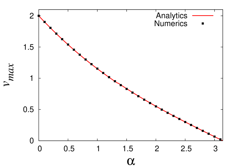
Figure 8: Plot of $v_{max}$ versus $\alpha$ for $T=0.5$ and $\gamma=1$. The solid red line shows the analytical result obtained from Eq. (103), while the black squares show the result obtained numerically from a study of the propagation of a particle as discussed in the text.

We now study the time evolution of a one-particle state, where the particle is initially at one particular site in the middle of a long chain with $N$ sites. Taking this site to be $n=0$, the initial state is given by

$$|\psi(0)\rangle~{}=~{}\int_{-\pi}^{\pi}~{}\frac{dk}{2\pi}~{}|k\rangle,$$ (104)

where we have taken the limit $N\to\infty$ so that $k$ is now a continuous variable. Upon evolving this for a time $T$ (but before acting with a $\delta$-function kick), $|k\rangle\to e^{i2\gamma T\cos k}|k\rangle$. The wave function at site $n$ is then

$$\psi_{n}(T)~{}=~{}\int_{-\pi}^{\pi}~{}\frac{dk}{2\pi}~{}e^{i(kn+2\gamma T\cos k)}.$$ (105)

This integral gives a Bessel function abram72 and we find that the probability of finding the particle at site $n$ is

$$|\psi_{n}(T)|^{2}~{}=~{}|J_{|n|}(2\gamma T)|^{2}.$$ (106)

This probability remains unchanged when the particle is then given a kick with an arbitrary strength $\alpha$, since a kick only changes the phase of $\psi_{n}$ by $e^{-i\alpha}$ on sites belonging to the $A$ sublattice. We therefore conclude that Floquet evolution for one time period spreads out the probability from the initial value of 1 at site $n=0$ to the expression given in Eq. (106).

For a given value of $2\gamma T$, it is known that $J_{|n|}(2\gamma T)$ rapidly goes to zero when $|n|$ becomes much larger than $2\gamma T$. Namely, abram72

$$J_{|n|}(2\gamma T)~{}\sim~{}\frac{1}{\sqrt{2\pi|n|}}~{}\left(\frac{e\gamma T}{|n|}\right)^{|n|}$$ (107)

for $|n|\gg 2\gamma T$. Eq. (106) therefore implies that the particle spreads out a distance of the order of $2\gamma T$ in time $T$; this is consistent with the fact that $v_{max}=2\gamma$ for a particle with the dispersion $\epsilon_{k}=2\gamma\cos k$. To make this more precise, we calculate the square of the width of the wave function at time $t$,

$$m_{2}(t)~{}\equiv~{}\sum_{n=-\infty}^{\infty}~{}n^{2}~{}|\psi_{n}(t)|^{2}.$$ (108)

Using the identity $\sum_{n=1}^{\infty}n^{2}[J_{n}(x)]^{2}=x^{2}/4$ for real $x$, we see from Eq. (106) that

$$m_{2}(T)~{}=~{}\frac{1}{2}~{}v_{max}^{2}T^{2},$$ (109)

where $v_{max}=2\gamma$.

We now study what happens to $m_{2}$ at integer multiples of $T$ up to very large times. Fig. 9 shows a plot of $m_{2}$ versus $t=nT$ for $\alpha=3.12$, $T=0.5$ and $\gamma=1$. Since $\alpha$ is close to $\pi$, the particle should be almost dynamically localized. We indeed see that $m_{2}$ remains of order 1 up to a large time $t$ although there are pronounced oscillations between odd and even integer values of $t/T$. Beyond that large time, however, odd and even integer values of $t/T$ give the same values of $m_{2}$. For such large times, a fit of the form

$$m_{2}~{}=~{}A~{}t^{p}$$ (110)

gives $p=2.0$. Fig. 8 compares the dependence of $v_{max}$ on $\alpha$ as obtained analytically from Eq. (103) (solid red line) and the dependence of $\sqrt{2A}$ on $\alpha$ as found numerically by fitting the large time behavior in Fig. 9 to the form in Eq. (110) (black squares), for $\gamma=1$ and $T=0.5$. The fact that the two match perfectly means that the parameter $A$ in Eq. (110) is equal to $v_{max}^{2}/2$ for all values of $\alpha$.

We can understand the time-dependence of $m_{2}$ for both small and large times as follows. We begin with Eq. (101). For $\alpha$ close to $\pi$, the leading order form of $U_{k}$ is given by

$$U_{k} \simeq \exp[-~{}\frac{i\pi}{2}~{}(I~{}+~{}\sigma^{x})]~{}\exp[i2\gamma T\cos k~{}\sigma^{z}]$$ (111)

$$= -~{}\cos(2\gamma T\cos k)~{}\sigma^{x}~{}-~{}\sin(2\gamma T\cos k)~{}\sigma^{y}.$$

Acting with $U_{k}$ on the column $(1,1)^{T}$ (which corresponds to the initial wave function $|k\rangle+|k+\pi\rangle$ given in Eq. (104)), we get $(-e^{-i2\gamma T\cos k},-e^{i2\gamma T\cos k})^{T}$ which corresponds to the wave function $-e^{-i2\gamma T\cos k}|k\rangle-e^{i2\gamma T\cos k}|k+\pi\rangle$. This is the same as the wave function in Eq. (105); this implies that $m_{2}(T)=(2\gamma T)^{2}/2$. Next, Eq. (111) implies that $U_{k}^{2}\simeq I$. We therefore have $U_{k}^{2p+1}\simeq U_{k}$ while $U_{k}^{2p}~{}\simeq I$ for any integer $p$. This would imply that $\psi((2p+1)T)\simeq\psi(T)$ so that $m_{2}((2p+1)T)\simeq(2\gamma T)^{2}/2$, while $\psi(2pT)\simeq\psi(0)$ so that $m_{2}(2pT)\simeq 0$. Thus $m_{2}$ is expected to alternate between $(2\gamma T)^{2}/2$ and a small number as $t/T$ alternates between odd and even integers. This agrees with what we see in Fig. 9 till $t/T$ reaches a large value of about 90; beyond this time $m_{2}$ has the same value for odd and even integer values of $t/T$ and increases quadratically with $t$. We can estimate the value of $t/T$ where this behavior begins as follows.

For $\alpha=\pi-\eta$, where $\eta$ is small, we find from Eq. (101) that

$$U_{k}^{2}~{}=~{}e^{i\eta}~{}\exp[i\eta\cos(2\gamma T\cos k)~{}\{\cos(2\gamma T\cos k)~{}\sigma^{x}~{}+~{}\sin(2\gamma T\cos k)~{}\sigma^{y}\}]$$ (112)

up to first order in $\eta$. We can compare this with the value of $U_{k}$ for $\alpha=\pi$ which, from Eq. (111), is given by

$$U_{k}~{}=~{}i~{}\exp[\frac{i\pi}{2}~{}\{\cos(2\gamma T\cos k)~{}\sigma^{x}~{}+~{}\sin(2\gamma T\cos k)~{}\sigma^{y}\}].$$ (113)

We have seen above, time evolution with $U_{k}$ gives $m_{2}(T)=(2\gamma T)^{2}/2$. Ignoring the $k$-independent phases in Eqs. (112-113) which do not affect the value of $m_{2}$, we see that the form of $U_{k}^{2p}$ will become identical to the form of $U_{k}$ when $2p=t/T$ is given by

$$p\eta\cos(2\gamma T\cos k)~{}=~{}\frac{\pi}{2}.$$ (114)

It is clear that the value of $p$ depends on $k$. However, the ballistic motion that is visible for $t\gtrsim 90$ in Fig. 9 is dominated by the values of $k$ where $v_{g}(k)=v_{max}$. For $\alpha=3.12$ (hence $\eta=\pi-3.12$), $T=0.5$ and $\gamma=1$, we find from Eq. (103) that $v_{g}=v_{max}$ for $k=0.829$ and $2.313$ (these add up to $\pi$). At these values of $k$, we have $\cos(2\gamma T\cos k)=0.780$; we then get $p=(\pi/2)/(0.780\times\eta)=93$. We see from Fig. 9 that $t\simeq 2\times 93\times T=93$ does approximately give the point at which the values of $m_{2}$ for odd and even integer values of $t/T$ merge and the ballistic motion begins.

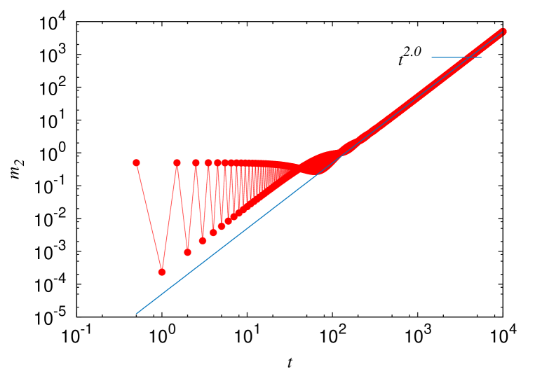
Figure 9: Plot of $m_{2}$ versus $t$ for $\alpha=3.12$, $T=0.5$ and $\gamma=1$. The particle is initially at a site in the middle of a system with 2000 sites. At short times, $m_{2}$ alternates between two values depending on whether $t/T$ is an odd or even integer. At long times, a power law fit between $m_{2}$ and $t$ shows that $m_{2}$ increases as $t^{2.0}$, implying that the particle is moving ballistically.

We conclude that for $\alpha$ close to $\pi$, a single particle remains dynamically localized up to a large time of order $1/|\pi-\alpha|$; up to this time $m_{2}$ alternates between two values, one of order $(2\gamma T)^{2}/2$ and the other of order zero, for odd and even values of $t/T$. Beyond that large time, $m_{2}$ increases quadratically with time indicating that the particle moves ballistically with a velocity $v_{max}$ which is of order $|\pi-\alpha|$. (The initial oscillations in $m_{2}$ are similar to those seen for other quantities in some recent papers on Floquet time crystals lazarides14d ; keyser16 ; else16a ; else16b ).

As another example of a perturbation, we consider what happens if there is disorder in the hopping amplitudes and the system is given $\delta$-function kicks with $\alpha=\pi$. Namely, the Hamiltonian is

$$H~{}=~{}\sum_{n=1}^{N}~{}t_{n,n+1}~{}(c_{n}^{\dagger}c_{n+1}~{}+~{}H.c.),$$ (115)

where $t_{n,n+1}$ can have some randomness. If this is kicked with an operator of the form $U_{K}=e^{-i\pi N_{A}}$, we find that the time evolution operator for two time periods is given by

$$U^{2} = e^{-i\pi N_{A}}~{}e^{-iHT}~{}e^{-i\pi N_{A}}~{}e^{-iHT}$$ (116)

$$= I$$

since $e^{-i\pi N_{A}}$ anticommutes with $(c_{n}^{\dagger}c_{n+1}+H.c.)$. Hence a particle will be dynamically localized after every integer multiple of $2T$.

VIII Concluding remarks

In this paper, we have examined the effects of interactions in bipartite lattice systems where periodic $\delta$-function kicks applied to the sublattice potential with a strength $\alpha=\pi$ lead to dynamical localization if we view the system stroboscopically. We have shown that interactions can generate new kinds of hoppings between nearest- and next-nearest-neighbor sites which depend on the occupation numbers on some nearby sites. These hoppings give rise to a variety of interesting effects.

We began by describing a formalism for calculating the effective Floquet Hamiltonian in an expansion in powers of $T$. We then calculated the Hamiltonian to second order in $T$ in three different models in one dimension. For spinless fermions with a nearest-neighbor interaction $V$, we showed that the two-particle sector has two branches of bound states: one branch which has a dispersion lying around $V$ and another branch with a dispersion around zero. We further showed that there are $n$-body bound states, with $n\geq 3$, which are dispersionless; hence they do not move with time. For the Hubbard model of spin-1/2 fermions with an on-site interaction $U$, we showed that the two-particle spin singlet sector has two branches of bound states with dispersions lying close to $U$ and zero respectively. In this model we do not find any $n$-body bound states if $n\geq 3$. For the Bose Hubbard model of bosons with on-site interaction $U$, we again found two branches of two-particle bounds states with quasienergies close to $U$ and zero, and dispersionless $n$-body bound states if $n\geq 3$. We also studied a special case of this model in which the interactions make states with occupancies $p$ and $p+1$ degenerate at each site. This allowed us to define a pseudo-spin-1/2 degree of freedom at each site, and we found an effective Hamiltonian which lies in the subspace of these states. For $p=0$, we obtained a particularly simple form of the effective Hamiltonian. We showed that a class of eigenstates of the effective Hamiltonian can be found exactly, and the degeneracy of the corresponding quasienergy grows exponentially with the system size. Finally, we showed that if the kicking strength $\alpha$ is slightly different from $\pi$, a particle remains dynamically localized for a long time of the order of $1/|\pi-\alpha|$ but then moves ballistically with a maximum velocity of the order of $|\pi-\alpha|$.

Turning to possible experimental realizations of the models studied in this paper, we note that a dynamical localization-to-delocalization transition has been observed in a quantum kicked rotor. Such a system is realized by placing cold atoms in a pulsed standing wave; the transition is detected by measuring the number of atoms which have zero velocity when a quasiperiodic driving is applied ringot00 . Given that cold atom systems provide a versatile platform for simulating a wide variety of condensed matter systems, our paper shows that a combination of periodic driving and interactions can lead to a variety of remarkable phenomena.

We would like to end by pointing out some possible directions for future studies.

(i) It would be interesting to study if dynamical localization induced by periodic driving along with interactions can give rise to topological phases. We note that in Ref. mikami16, , it was shown that circularly polarized light (which corresponds to simple harmonic driving) can give rise to transitions to topological phases; the effect of interactions was then studied within dynamical mean-field theory. One can similarly investigate if periodic $\delta$-function kicks and interactions can drive topological phase transitions.

(ii) A generalization of our results to bipartite lattice models in higher dimensions may be interesting. It is not difficult to carry out a perturbative expansion of the effective Hamiltonian in any dimension. However, it may be more difficult to find bound states of two or more particles and to study the time evolution of few-particle states in higher than one dimension.

(iii) We have mainly concentrated on the dynamics of systems with a small number of particles. (An exception to this was the analysis in Secs. VI A and B where we looked at systems with an arbitrary number of particles). It may be useful to study the thermodynamics of a system with a finite filling fraction of particles. In particular, one can look at the possible phases of such systems (for instance, if they are metals, superfluids or insulators) and the nature of the excitations in the different phases. We note that such a study requires us to couple the system to a thermal reservoir, and the phases of the system may depend on the form of the system-reservoir couplings iadecola15a ; iadecola15b . Some recent papers have studied scattering processes and heating effects in periodically driven systems with interactions bilitewski15 ; genske15 .

(iv) We have seen in some cases that there are few-particle bound states with a dispersionless spectrum. This raises the question of whether the spectrum would continue to be so simple if we expand the effective Hamiltonian to higher than second order in $T$. Another interesting question to ask is: what is the time scale up to which the results obtained from the effective Hamiltonian derived to order $T^{2}$ remain accurate? An answer to this has been provided in Ref. kuwahara16, where a time scale is found up to which the results obtained using an effective Hamiltonian derived to order $T^{n}$ and the exact Floquet operator match well and beyond which they start disagreeing.

We also know that the models of interacting spinless and spin-1/2 fermions are Bethe ansatz solvable mattis93 ; sutherland04 . We may investigate if this has any implications for the properties of the system in the presence of periodic $\delta$-function kicking.

(v) It is interesting to compare our results with those found in many-body localization (MBL). In MBL, the localization is due to the spatial disorder and/or interactions. Some studies have then looked at the effects of periodic driving on the MBL state ponte15a ; lazarides14c ; ponte15b . Our motivation and study are completely distinct. We begin with a system which is completely dynamically localized even in the absence of disorder. We then probe the effect of interactions on systems with a few particles. The few-particle bound states that we find are again dynamically localized. Unlike MBL systems, the driving protocol plays the essential role here of localizing the particles. It would be interesting to study an interplay of dynamical localization due to driving, spatial localization due to disorder, and interactions.

Appendix A Mathematical Identities

We begin with the identity

$$e^{X}e^{Y}~{}=~{}e^{Y+[X,Y]+\frac{1}{2!}[X,[X,Y]]+\frac{1}{3!}[X,[X,[X,Y]]]+\cdots}~{}e^{X}.$$ (117)

If $[X,Y]=\gamma Y$, where $\gamma$ is a number, then the above equation implies that

$$e^{X}e^{Y}=e^{(e^{\gamma})Y}e^{X}.$$ (118)

If $[X,Z]=0$ along with $[X,Y]=\gamma Y$, then we get

$$e^{X}e^{Y+Z}~{}=~{}e^{(e^{\gamma})Y+Z}~{}e^{X}.$$ (119)

The Baker-Campbell-Hausdorff formula gives

$$e^{X}e^{Y}~{}=~{}e^{X+Y+\frac{1}{2}[X,Y]+\frac{1}{12}([X,[X,Y]]+[Y,[Y,X]])+\cdots},$$ (120)

which implies that

$$\ln(e^{X}e^{Y})~{}=~{}X~{}+~{}Y~{}+~{}\frac{1}{2}[X,Y]~{}+~{}\frac{1}{12}([X,[X,Y]]~{}+~{}[Y,[Y,X]])~{}+~{}\cdots.$$ (121)

If $X=C+D$ and $Y=C-D$, then

$$\ln(e^{C+D}e^{C-D}) = 2C~{}+~{}[D,C]~{}+~{}\frac{1}{3}([C,D]D+D[D,C])~{}+~{}\cdots$$ (122)

$$= 2C~{}+~{}[D,C]~{}+~{}\frac{1}{3}[D,[D,C]]~{}+~{}\cdots.$$

Finally, for fermion operators we know that

$$[n_{j},c_{j}]~{}=~{}-c_{j}~{}~{}~{}{\rm and}~{}~{}~{}[n_{j},c^{\dagger}_{j}]=c^{\dagger}_{j},$$ (123)

where $n_{j}=c^{\dagger}_{j}c_{j}$. For bosons

$$[b_{i},b^{\dagger}_{j}]~{}=~{}\delta_{ij},$$ (124)

and this gives the same commutation relations between $n_{j}=b^{\dagger}_{j}b_{j}$ and $b_{j},~{}b^{\dagger}_{j}$ as in Eq. (123).

Appendix B Derivation of effective Hamiltonian for the bosonic model

We now present the details of the calculation of the effective Hamiltonian when the occupancies $p$ and $p+1$ of a site are degenerate.

Second order processes involving two sites:

The various processes will be shown below as tables. Each table will show an initial (or intermediate) state $I$ and an intermediate (or final) state $F$, with $I_{j}$ and $F_{j}$ denoting the number of particles at site $j$ in the $I$ and $F$ states respectively.

1.

$$\begin{array}[]{|c|c||c|c||c|}\hline\cr I_{j}&I_{j+1}&F_{j}&F_{j+1}&Amplitude\\ \hline\cr\hline\cr p&p&p-1&p+1&\frac{i\gamma TU}{2}~{}\sqrt{p}\sqrt{p+1}\\ p-1&p+1&p&p&-\frac{i\gamma TU}{2}~{}\sqrt{p}\sqrt{p+1}\\ \hline\cr\end{array}$$ (125)

• The energy denominator coming from the difference of the unperturbed energies of the initial and final states is $-U$.

• This process can occur in two ways, as we can have $F_{j}=p+1,~{}F_{j+1}=p-1$. So we get a total contribution

  $$2~{}\left(\frac{i\gamma TU}{2}\sqrt{p}\sqrt{p+1}\right)~{}\left(\frac{-i\gamma TU}{2}\sqrt{p}\sqrt{p+1}\right)~{}\left(\frac{1}{-U}\right)~{}=~{}-\frac{p(p+1)\gamma^{2}T^{2}U}{2}.$$ (126)

2.

$$\begin{array}[]{|c|c||c|c||c|}\hline\cr I_{j}&I_{j+1}&F_{j}&F_{j+1}&Amplitude\\ \hline\cr\hline\cr p&p+1&p-1&p+2&i\gamma TU~{}\sqrt{p}\sqrt{p+2}\\ p-1&p+2&p&p+1&-i\gamma TU~{}\sqrt{p}\sqrt{p+2}\\ \hline\cr\end{array}$$ (127)

• The energy denominator is $-2U$.

• The total contribution is

  $$-\frac{p(p+2)\gamma^{2}T^{2}U}{2}.$$ (128)

• A similar process occurs when the initial state has $I_{j}=p+1,~{}I_{j+1}=p$.

3.

$$\begin{array}[]{|c|c||c|c||c|}\hline\cr I_{j}&I_{j+1}&F_{j}&F_{j+1}&Amplitude\\ \hline\cr\hline\cr p+1&p+1&p&p+2&\frac{i\gamma TU}{2}~{}\sqrt{p+1}\sqrt{p+2}\\ p&p+2&p+1&p+1&-\frac{i\gamma TU}{2}~{}\sqrt{p+1}\sqrt{p+2}\\ \hline\cr\end{array}$$ (129)

• The energy denominator is $-U$.

• This process can occur in two possible ways. So the total contribution is

  $$-\frac{(p+1)(p+2)\gamma^{2}T^{2}U}{2}.$$ (130)

We now find that all the above terms can be fitted to an expression of the form

$$a_{1}~{}\sigma^{z}_{j}~{}+~{}a_{2}~{}\sigma^{z}_{j+1}~{}+~{}a_{3}~{}\sigma^{z}_{j}\sigma^{z}_{j+1}~{}+~{}a_{4}.$$ (131)

Comparing this expression with the contributions given above, we obtain

$$-a_{1}-a_{2}+a_{3}+a_{4} = -\frac{\gamma^{2}T^{2}U}{2}~{}p(p+1),$$

$$-a_{1}+a_{2}-a_{3}+a_{4} = -\frac{\gamma^{2}T^{2}U}{2}~{}p(p+2),$$

$$a_{1}-a_{2}-a_{3}+a_{4} = -\frac{\gamma^{2}T^{2}U}{2}~{}p(p+2),$$

$$a_{1}+a_{2}+a_{3}+a_{4} = -\frac{\gamma^{2}T^{2}U}{2}~{}(p+1)(p+2).$$ (132)

These imply

$$a_{1} = -\frac{\gamma^{2}T^{2}U}{4}~{}(p+1),$$

$$a_{2} = -\frac{\gamma^{2}T^{2}U}{4}~{}(p+1),$$

$$a_{3} = -\frac{\gamma^{2}T^{2}U}{4},$$

$$a_{4} = -\frac{\gamma^{2}T^{2}U}{4}~{}(2p^{2}+4p+1).$$ (133)

We therefore have the following terms in $H_{eff}$ so far

$$-\frac{\gamma^{2}T^{2}U}{4}~{}\Bigl{[}~{}(p+1)~{}(\sigma^{z}_{j}+\sigma^{z}_{j+1})~{}+~{}\sigma^{z}_{j}\sigma^{z}_{j+1}~{}+~{}(2p^{2}+4p+1)\Bigr{]}.$$ (134)

Second order processes involving three sites:

1.

$$\begin{array}[]{|c|c|c||c|c|c||c|}\hline\cr I_{j}&I_{j+1}&I_{j+2}&F_{j}&F_{j+1}&F_{j+2}&Amplitude\\ \hline\cr p&p&p&-&-&-&-\\ \hline\cr\end{array}$$ (135)

The symbol $-$ in the table means that the terms in Eq. (64) take the state $(I_{j},I_{j+1},I_{j+2})$ to a state which is not relevant to the calculation of $H_{eff}$.

2.

$$\begin{array}[]{|c|c|c||c|c|c||c|}\hline\cr I_{j}&I_{j+1}&I_{j+2}&F_{j}&F_{j+1}&F_{j+2}&Amplitude\\ \hline\cr\hline\cr p&p&p+1&p+1&p-1&p+1&\frac{i\gamma TU}{2}~{}\sqrt{p}\sqrt{p+1}\\ p+1&p-1&p+1&p+1&p&p&-\frac{i\gamma TU}{2}~{}\sqrt{p}\sqrt{p+1}\\ \hline\cr\end{array}$$ (136)

• The energy denominator is $-U$.

• The total contribution is

  $$-\frac{p(p+1)\gamma^{2}T^{2}U}{4}.$$ (137)

3.

$$\begin{array}[]{|c|c|c||c|c|c||c|}\hline\cr I_{j}&I_{j+1}&I_{j+2}&F_{j}&F_{j+1}&F_{j+2}&Amplitude\\ \hline\cr p&p+1&p&-&-&-&-\\ \hline\cr\end{array}$$ (138)

The terms in Eq. (64) take the state $(I_{j},I_{j+1},I_{j+2})$ to a state which is not relevant to the calculation of $H_{eff}$.

4.

$$\begin{array}[]{|c|c|c||c|c|c||c|}\hline\cr I_{j}&I_{j+1}&I_{j+2}&F_{j}&F_{j+1}&F_{j+2}&Amplitude\\ \hline\cr\hline\cr p&p+1&p+1&p&p+2&p&\frac{i\gamma TU}{2}~{}\sqrt{p+1}\sqrt{p+2}\\ p&p+2&p&p+1&p+1&p&-\frac{i\gamma TU}{2}~{}\sqrt{p+1}\sqrt{p+2}\\ \hline\cr\end{array}$$ (139)

• The energy cost from the on-site energy is $-U$.

• The total contribution is

  $$-\frac{(p+1)(p+2)\gamma^{2}T^{2}U}{4}.$$ (140)

5.

$$\begin{array}[]{|c|c|c||c|c|c||c|}\hline\cr I_{j}&I_{j+1}&I_{j+2}&F_{j}&F_{j+1}&F_{j+2}&Amplitude\\ \hline\cr\hline\cr p+1&p&p&p+1&p-1&p+1&\frac{i\gamma TU}{2}~{}\sqrt{p}\sqrt{p+1}\\ p+1&p-1&p+1&p&p&p+1&-\frac{i\gamma TU}{2}~{}\sqrt{p}\sqrt{p+1}\\ \hline\cr\end{array}$$ (141)

• The energy denominator is $-U$.

• The total contribution is

  $$-\frac{p(p+1)\gamma^{2}T^{2}U}{4}.$$ (142)

6.

$$\begin{array}[]{|c|c|c||c|c|c||c|}\hline\cr I_{j}&I_{j+1}&I_{j+2}&F_{j}&F_{j+1}&F_{j+2}&Amplitude\\ \hline\cr p+1&p&p+1&-&-&-&-\\ \hline\cr\end{array}$$ (143)

The terms in Eq. (64) take the state $(I_{j},I_{j+1},I_{j+2})$ to a state which is not relevant to the calculation of $H_{eff}$.

7.

$$\begin{array}[]{|c|c|c||c|c|c||c|}\hline\cr I_{j}&I_{j+1}&I_{j+2}&F_{j}&F_{j+1}&F_{j+2}&Amplitude\\ \hline\cr\hline\cr p+1&p+1&p&p&p+2&p&\frac{i\gamma TU}{2}~{}\sqrt{p+1}\sqrt{p+2}\\ p&p+2&p&p&p+1&p+1&-\frac{-i\gamma TU}{2}~{}\sqrt{p+1}\sqrt{p+2}\\ \hline\cr\end{array}$$ (144)

• The energy denominator $-U$.

• The total contribution is

  $$-\frac{(p+1)(p+2)\gamma^{2}T^{2}U}{4}.$$ (145)

8.

$$\begin{array}[]{|c|c|c||c|c|c||c|}\hline\cr I_{j}&I_{j+1}&I_{j+2}&F_{j}&F_{j+1}&F_{j+2}&Amplitude\\ \hline\cr p+1&p+1&p+1&-&-&-&-\\ \hline\cr\end{array}$$ (146)

The terms in Eq. (64) take the state $(I_{j},I_{j+1},I_{j+2})$ to a state which is not relevant to the calculation of $H_{eff}$.

Looking at the processes in items 2, 4, 5 and 7 above, we see that all of them interchange $n_{j}$ and $n_{j+2}$ keeping $n_{j+1}$ unchanged.

Direct contributions from terms of order $\gamma^{2}T^{2}U$ involving three sites:

$$\begin{array}[]{|c|c|c||c|c|c||c|}\hline\cr I_{j}&I_{j+1}&I_{j+2}&F_{j}&F_{j+1}&F_{j+2}&Amplitude\\ \hline\cr\hline\cr p&p&p+1&p+1&p&p&\frac{\gamma^{2}T^{2}U}{3}~{}p(p+1)\\ p+1&p&p&p&p&p+1&\frac{\gamma^{2}T^{2}U}{6}~{}p(p+1)\\ p&p+1&p+1&p+1&p+1&p&\frac{\gamma^{2}T^{2}U}{6}~{}(p+2)(p+1)\\ p+1&p+1&p&p&p+1&p+1&\frac{\gamma^{2}T^{2}U}{6}~{}(p+2)(p+1)\\ \hline\cr\end{array}$$ (147)

We see that these processes also interchange $n_{j}$ and $n_{j+2}$ keeping $n_{j+1}$ unchanged. Adding up the contributions of the second order processes and direct contributions involving three sites, we obtain the following table.

$$\begin{array}[]{|c|c|c||c|c|c||c|}\hline\cr I_{j}&I_{j+1}&I_{j+2}&F_{j}&F_{j+1}&F_{j+2}&Amplitude\\ \hline\cr\hline\cr p&p&p+1&p+1&p&p&(\frac{1}{3}-\frac{1}{4})\gamma^{2}T^{2}U~{}p(p+1)=\frac{\gamma^{2}T^{2}U}{12}~{}p(p+1)\\ p+1&p&p&p&p&p+1&\frac{\gamma^{2}T^{2}U}{12}~{}p(p+1)\\ p&p+1&p+1&p+1&p+1&p&\frac{\gamma^{2}T^{2}U}{12}~{}(p+2)(p+1)\\ p+1&p+1&p&p&p+1&p+1&\frac{\gamma^{2}T^{2}U}{12}~{}(p+2)(p+1)\\ \hline\cr\end{array}$$ (148)

We now recall from Eq. (78) that $n_{j}$ is related to the pseudo-spin $\sigma^{z}_{j}$. Hence the terms in (148) can be fitted to a three-spin interaction of the form

$$(b_{1}~{}+~{}b_{2}\sigma^{z}_{j+1})~{}(\sigma^{+}_{j}\sigma^{-}_{j+2}~{}+~{}\sigma^{-}_{j}\sigma^{+}_{j+2}).$$ (149)

To be explicit, we find that this part of $H_{eff}$ is given by

$$\frac{\gamma^{2}T^{2}U}{12}(p+1)(p+1+\sigma^{z}_{j+1})(\sigma^{+}_{j}\sigma^{-}_{j+2}+\sigma^{-}_{j}\sigma^{+}_{j+2}).$$ (150)

Direct contributions from terms of order $\gamma^{2}T^{2}U$ involving two sites:

Finally, we find that the terms in Eq. (65) contribute to terms in $H_{eff}$ which involve only two sites. Using Eq. (78), we find that

$$-\frac{\gamma^{2}T^{2}U}{3}~{}\sum_{j}~{}\Big{[}2n_{j}(n_{j}-1)-4n_{j}n_{j+1}\Big{]}$$ (151)

$$= \frac{\gamma^{2}T^{2}U}{3}~{}\sum_{j}~{}\left[2(p+1)\sigma^{z}_{j}+\sigma^{z}_{j}\sigma^{z}_{j+1}+(2p^{2}+4p+1)\right].$$

Putting together Eqs. (134), (150) and (151), we find the complete effective Hamiltonian shown in Eq. (80) in the main text.

References

- (1)
- (2) F. Grossmann, T. Dittrich, P. Jung, and P. Hänggi, Phys. Rev. Lett. 67, 516 (1991).
- (3) Y. Kayanuma, Phys. Rev. A 50, 843 (1994).
- (4) V. Mukherjee, A. Dutta, and D. Sen, Phys. Rev. B 77, 214427 (2008).
- (5) V. Mukherjee and A. Dutta, J. Stat. Mech. (2009) P05005.
- (6) A. Das, Phys. Rev. B 82, 172402 (2010).
- (7) A. Russomanno, A. Silva, and G. E. Santoro, Phys. Rev. Lett. 109, 257201 (2012).
- (8) L. D’Alessio and A. Polkovnikov, Annals of Physics 333, 19 (2013).
- (9) M. Bukov, L. D’Alessio, and A. Polkovnikov, Advances in Physics 64, 139 (2015).
- (10) T. Nag, S. Roy, A. Dutta, and D. Sen, Phys. Rev. B 89, 165425 (2014).
- (11) T. Nag, D. Sen, and A. Dutta, Phys. Rev. A 91, 063607 (2015).
- (12) A. Agarwala, U. Bhattacharya, A. Dutta, and D. Sen, Phys. Rev. B 93, 174301 (2016).
- (13) S. Sharma, A. Russomanno, G. E. Santoro, and A. Dutta, EPL 106, 67003 (2014).
- (14) A. Russomanno, S. Sharma, A. Dutta, and G. E. Santoro, J. Stat. Mech. (2015) P08030.
- (15) A. Lazarides, A. Das, and R. Moessner, Phys. Rev. Lett. 112, 150401 (2014).
- (16) A. Dutta, G. Aeppli, B. K. Chakrabarti, U. Divakaran, T. Rosenbaum and D. Sen, Quantum Phase Transitions in Transverse Field Spin Models: From Statistical Physics to Quantum Information (Cambridge University Press, Cambridge, 2015).
- (17) Z. Gu, H. A. Fertig, D. P. Arovas, and A. Auerbach, Phys. Rev. Lett. 107, 216601 (2011).
- (18) T. Kitagawa, T. Oka, A. Brataas, L. Fu, and E. Demler, Phys. Rev. B 84, 235108 (2011).
- (19) E. Suárez Morell and L. E. F. Foa Torres, Phys. Rev. B 86, 125449 (2012).
- (20) M. A. Sentef, M. Claassen, A. F. Kemper, B. Moritz, T. Oka, J. K. Freericks, and T. P. Devereaux, Nature Commun. 6, 7047 (2015).
- (21) T. Kitagawa, E. Berg, M. Rudner, and E. Demler, Phys. Rev. B 82, 235114 (2010).
- (22) N. H. Lindner, G. Refael, and V. Galitski, Nature Phys. 7, 490 (2011).
- (23) L. Jiang, T. Kitagawa, J. Alicea, A. R. Akhmerov, D. Pekker, G. Refael, J. I. Cirac, E. Demler, M. D. Lukin, and P. Zoller, Phys. Rev. Lett. 106, 220402 (2011).
- (24) M. Trif and Y. Tserkovnyak, Phys. Rev. Lett. 109, 257002 (2012).
- (25) A. Gomez-Leon and G. Platero, Phys. Rev. B 86, 115318 (2012), and Phys. Rev. Lett. 110, 200403 (2013).
- (26) B. Dóra, J. Cayssol, F. Simon, and R. Moessner, Phys. Rev. Lett. 108, 056602 (2012).
- (27) J. Cayssol, B. Dora, F. Simon, and R. Moessner, Phys. Status Solidi RRL 7, 101 (2013).
- (28) D. E. Liu, A. Levchenko, and H. U. Baranger, Phys. Rev. Lett. 111, 047002 (2013).
- (29) Q.-J. Tong, J.-H. An, J. Gong, H.-G. Luo, and C. H. Oh, Phys. Rev. B 87, 201109(R) (2013).
- (30) M. S. Rudner, N. H. Lindner, E. Berg, and M. Levin, Phys. Rev. X 3, 031005 (2013).
- (31) Y. T. Katan and D. Podolsky, Phys. Rev. Lett. 110, 016802 (2013).
- (32) N. H. Lindner, D. L. Bergman, G. Refael, and V. Galitski, Phys. Rev. B 87, 235131 (2013).
- (33) A. Kundu and B. Seradjeh, Phys. Rev. Lett. 111, 136402 (2013).
- (34) V. M. Bastidas, C. Emary, G. Schaller, A. Gómez-León, G. Platero, and T. Brandes, arXiv:1302.0781.
- (35) T. L. Schmidt, A. Nunnenkamp, and C. Bruder, New J. Phys. 15, 025043 (2013).
- (36) A. A. Reynoso and D. Frustaglia, Phys. Rev. B 87, 115420 (2013).
- (37) C.-C. Wu, J. Sun, F.-J. Huang, Y.-D. Li, and W.-M. Liu, EPL 104, 27004 (2013).
- (38) M. Thakurathi, A. A. Patel, D. Sen, and A. Dutta, Phys. Rev. B 88, 155133 (2013).
- (39) P. M. Perez-Piskunow, G. Usaj, C. A. Balseiro, and L. E. F. Foa Torres, Phys. Rev. B 89, 121401(R) (2014).
- (40) G. Usaj, P. M. Perez-Piskunow, L. E. F. Foa Torres, and C. A. Balseiro, Phys. Rev. B 90, 115423 (2014).
- (41) P. M. Perez-Piskunow, L. E. F. Foa Torres, and G. Usaj, Phys. Rev. A 91, 043625 (2015).
- (42) M. D. Reichl and E. J. Mueller, Phys. Rev. A 89, 063628 (2014).
- (43) M. Thakurathi, K. Sengupta, and D. Sen, Phys. Rev. B 89, 235434 (2014).
- (44) T. Kitagawa, M. A. Broome, A. Fedrizzi, M. S. Rudner, E. Berg, I. Kassal, A. Aspuru-Guzik, E. Demler, and A. G. White, Nat. Commun. 3, 882 (2012).
- (45) M. C. Rechtsman, J. M. Zeuner, Y. Plotnik, Y. Lumer, D. Podolsky, S. Nolte, F. Dreisow, M. Segev, and A. Szameit, Nature (London) 496, 196 (2013).
- (46) M. C. Rechtsman, Y. Plotnik, J. M. Zeuner, D. Song, Z. Chen, A. Szameit, and M. Segev, Phys. Rev. Lett. 111, 103901 (2013).
- (47) Y. Plotnik, M. C. Rechtsman, D. Song, M. Heinrich, J. M. Zeuner, S. Nolte, Y. Lumer, N. Malkova, J. Xu, A. Szameit, Z. Chen, and M. Segev, Nature Materials 13, 57 (2014).
- (48) L. Tarruell, D. Greif, T. Uehlinger, G. Jotzu, and T. Esslinger, Nature (London) 483, 302 (2012).
- (49) G. Jotzu, M. Messer, R. Desbuquois, M. Lebrat, T. Uehlinger, D. Greif, and T. Esslinger, Nature (London) 515, 237 (2014).
- (50) A. Eckardt, C. Weiss, and M. Holthaus, Phys. Rev. Lett. 95, 260404 (2005).
- (51) A. Rapp, X. Deng, and L. Santos, Phys. Rev. Lett. 109, 203005 (2012).
- (52) W. Zheng, B. Liu, J. Miao, C. Chin, and H. Zhai, Phys. Rev. Lett. 113, 155303 (2014).
- (53) S. Greschner, L. Santos, and D. Poletti, Phys. Rev. Lett. 113, 183002 (2014).
- (54) A. Lazarides, A. Das, and R. Moessner, Phys. Rev. E 90, 012110 (2014).
- (55) L. D’Alessio and M. Rigol, Phys. Rev. X 4, 041048 (2014).
- (56) P. Ponte, Z. Papić, F. Huveneers, and D. A. Abanin, Phys. Rev. Lett. 114, 140401 (2015).
- (57) A. Lazarides, A. Das, and R. Moessner, Phys. Rev. Lett. 115, 030402 (2015).
- (58) P. Ponte, A. Chandran, Z. Papić, and D. A. Abanin, Annals of Physics 353, 196 (2015).
- (59) A. Eckardt and E. Anisimovas, New J. Phys. 17, 093039 (2015).
- (60) M. Bukov, M. Kolodrubetz, and A. Polkovnikov, Phys. Rev. Lett. 116, 125301 (2016).
- (61) V. Khemani, A. Lazarides, R. Moessner, and S. L. Sondhi, Phys. Rev. Lett. 116, 250401 (2016).
- (62) C. W. von Keyserlingk, V. Khemani, and S. L. Sondhi, Phys. Rev. B 94, 085112 (2016).
- (63) D. V. Else, B. Bauer, and C. Nayak, Phys. Rev. Lett. 117, 090402 (2016).
- (64) D. V. Else, B. Bauer, and C. Nayak, arXiv:1607.05277.
- (65) A. P. Itin and M. I. Katsnelson, Phys. Rev. Lett. 115, 075301 (2015).
- (66) T. Mikami, S. Kitamura, K. Yasuda, N. Tsuji, T. Oka, and H. Aoki, Phys. Rev. B 93, 144307 (2016).
- (67) W. Su, M. N. Chen, L. B. Shao, L. Sheng, and D. Y. Xing, Phys. Rev. B 94, 075145 (2016).
- (68) M. Račiūnas, G. Žlabys, A. Eckardt, and E. Anisimovas, Phys. Rev. A 93, 043618 (2016).
- (69) F. Meinert, M. J. Mark, K. Lauber, A. J. Daley, and H.-C. Nägerl, Phys. Rev. Lett. 116, 205301 (2016).
- (70) P. Bordia, H. P. Lüschen, S. S. Hodgman, M. Schreiber, I. Bloch, and U. Schneider, Phys. Rev. Lett. 116, 140401 (2016).
- (71) P. Bordia, H. Lüschen, U. Schneider, M. Knap, and I. Bloch, arXiv:1607.07868v1.
- (72) S. Mukherjee, M. Valiente, N. Goldman, A. Spracklen, E. Andersson, P. Öhberg, and R. R. Thomson, Phys. Rev. A 94, 053853 (2016).
- (73) B. V. Chirikov, F. M. Izrailev, and D. L. Shepelyansky, Sov. Sci. Rev. C 2, 209 (1981).
- (74) S. Fishman, D. R. Grempel, and R. E. Prange, Phys. Rev. Lett. 49, 509 (1982).
- (75) H. Ammann, R. Gray, I. Shvarchuck, and N. Christensen, Phys. Rev. Lett. 80, 4111 (1998).
- (76) C. Tian, A. Altland, and M. Garst, Phys. Rev. Lett. 107, 074101 (2011).
- (77) E. P. L. van Nieuwenburg, J. M. Edge, J. P. Dahlhaus, J. Tworzydlo, and C. W. J. Beenakker, Phys. Rev. B 85, 165131 (2012).
- (78) P. L. Kapitza, Sov. Phys. JETP 21, 588 (1951).
- (79) H. W. Broer, I. Hoveijn, M. van Noort, C. Simon, and G. Vegter, Journal of Dynamics and Differential Equations, 16 897 (2004).
- (80) B. Horstmann, J. I. Cirac, and T. Roscilde, Phys. Rev. A. 76, 043625 (2007).
- (81) A. Roy and A. Das, Phys. Rev. B 91, 121106(R) (2015).
- (82) N. Regnault and B. A. Bernevig, Phys. Rev. X 1, 021014 (2011).
- (83) D. N. Sheng, Z.-C. Gu, K. Sun, and L. Sheng, Nature Commun. 2, 389 (2011).
- (84) T. Neupert, L. Santos, C. Chamon, and C. Mudry, Phys. Rev. Lett. 106, 236804 (2011).
- (85) Y.-F. Wang, Z.-C. Gu, C.-D. Gong, and D. N. Sheng, Phys. Rev. Lett. 107, 146803 (2011).
- (86) E. Tang, J.-W. Mei, and X.-G. Wen, Phys. Rev. Lett. 106, 236802 (2011).
- (87) S. Dasgupta, U. Bhattacharya, and A. Dutta, Phys. Rev. E 91, 052129 (2015).
- (88) R. Zitko, Comp. Phys. Comm. 182, 2259 (2011).
- (89) D. C. Mattis, The Many-Body Problem (World Scientific, Singapore, 1993).
- (90) B. Sutherland, Beautiful Models (World Scientific, Singapore, 2004).
- (91) R. I. Nepomechie and C. Wang, J. Phys. A 47, 505004 (2014).
- (92) P. R. Giri and T. Deguchi, J. Phys. A 48, 175207 (2015).
- (93) J. K. Freericks and H. Monien, Europhys. Lett. 26, 545 (1994).
- (94) R. K. Pathria, Statistical Mechanics (Butterworth-Heinemann, Oxford, 1996).
- (95) T. Bilitewski and N. R. Cooper, Phys. Rev. A 91, 033601 (2015).
- (96) M. Genske and A. Rosch, Phys. Rev. A 92, 062108 (2015).
- (97) T. Kuwahara, T. Mori, and K. Saito, Annals of Physics 367, 96 (2016).
- (98) E. H. Lieb and D. Robinson, Commun. Math. Phys. 28, 251 (1972).
- (99) M. Abramowitz and I. A. Stegun, Handbook of Mathematical Functions (Dover, New York, 1972).
- (100) J. Ringot, P. Szriftgiser, J. C. Garreau, and D. Delande, Phys. Rev. Lett. 85, 2741 (2000).
- (101) T. Iadecola and C. Chamon, Phys. Rev. B 91, 184301 (2015).
- (102) T. Iadecola, T. Neupert, and C. Chamon, Phys. Rev. B 91, 235133 (2015).