{felix.jaremo-lawin, per-erik.forssen, hannes.ovren}@liu.se
Efficient Multi-Frequency Phase Unwrapping using Kernel Density Estimation
Abstract
In this paper we introduce an efficient method to unwrap multi-frequency phase estimates for time-of-flight ranging. The algorithm generates multiple depth hypotheses and uses a spatial kernel density estimate (KDE) to rank them. The confidence produced by the KDE is also an effective means to detect outliers. We also introduce a new closed-form expression for phase noise prediction, that better fits real data. The method is applied to depth decoding for the Kinect v2 sensor, and compared to the Microsoft Kinect SDK and to the open source driver libfreenect2. The intended Kinect v2 use case is scenes with less than m range, and for such cases we observe consistent improvements, while maintaining real-time performance. When extending the depth range to the maximal value of m, we get about more valid measurements than libfreenect2. The effect is that the sensor can now be used in large depth scenes, where it was previously not a good choice. Code and supplementary material are available at http://www.cvl.isy.liu.se/research/datasets/kinect2-dataset/.
Keywords:
Time-of-flight, Kinect v2, kernel-density-estimation1 Introduction
Multi-frequency time-of-flight is a way to accurately estimate distance, that was originally invented for Doppler RADAR [1]. More recently it has also found an application in RGB-D sensors111RGB-D sensors output both colour (RGB) and depth (D) images. that use time-of-flight ranging, such as the Microsoft Kinect v2 [2].
Depth from time-of-flight requires very accurate time-of-arrival estimation. Amplitude modulation improves accuracy, by measuring phase shifts between the received and emitted signals, instead of time-of-arrival. However, a disadvantage with amplitude modulation is that it introduces a periodic depth ambiguity. By using multiple modulation frequencies in parallel, the ambiguity can be resolved in most cases, and the useful range can thus be extended.
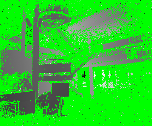
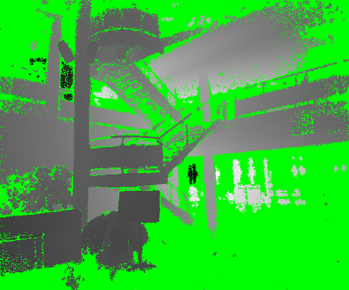
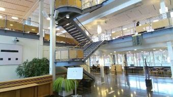
We introduce an efficient method to unwrap multi-frequency phase estimates for time-of-flight ranging. The algorithm uses kernel density estimation (KDE) in a spatial neighbourhood to rank different depth hypotheses. The KDE also doubles as a confidence measure which can be used to detect and suppress bad pixels. We apply our method to depth decoding for the Kinect v2 sensor. For large depth scenes we see a significant increase in coverage of about more valid pixels compared to libfreenect2. See figure 1 for a qualitative comparison. For 3D modelling with Kinect fusion [3], this results in fewer outlier points and more complete scene details. While the method is designed with the Kinect v2 in mind, it is also applicable to multi-frequency ranging techniques in general.
1.1 Related Work
The classic solution to the multi-frequency phase unwrapping problem, is to use the Chinese reminder theorem (CRT). This method is fast, but implicitly assumes noise free data, and in [1] it is demonstrated that by instead generating multiple unwrappings for each frequency, and then performing clustering along the range axis, better robustness to noise is achieved. However, due to its simplicity, CRT is still advocated, e.g. in [4, 5], and is also used in the Kinect v2 drivers.
Simultaneous unwrapping of multiple phases with different frequencies is a problem that also occurs in fringe pattern projection techniques [6, 5]. The algorithms are not fully equivalent though, as the phase is estimated by different means, and the relationship between phase and depth is different.
Another way to unwrap the time-of-flight phase shift is to use surface reflectivity constraints. As the amplitude associated with each phase measurement is a function of object distance and surface reflectivity, a popular approach in the literature is to assume locally constant reflectivity. Under this assumption, the depth can be unwrapped using e.g. a Markov Random Field (MRF) formulation with a data term and a reflectivity smoothness term. In [7], many different such unwrapping methods are discussed. A recent extension of this is [8], where distance, surface albedo and also the local surface normal are used to predict the reflectance.
The multi-frequency and reflectivity approaches are combined in [9] where a MRF with both reflectivity, and dual frequency data terms are used.
Detection of multipath interference (i.e. measurement problems due to light reflected from several different world locations reaching the same pixel) is studied in [10]. If four or more frequencies are used, pixels with multipath effects can be detected and suppressed. Recently in [11], a multipath detection algorithm based on blind source separation was applied to the Kinect v2. This required the firmware of the Kinect v2 to be modified to emit and receive at 5 frequencies instead of the default 3. As firmware modification currently requires reverse engineering of the transmission protocol we have not pursued this line of research.
In [12] a simulator for ToF measurements is developed and used to evaulate performance of a MRF that does simultaneous unwrapping and denoising using a wavelet basis. The performance on real data is however not shown.
Noise on the phase measurements is analyzed in [13] and it is suggested that the variance of phase is predicted by sensor variance divided by the phase amplitude squared. In this paper we derive a new model for phase noise that fits better with real data and utilize it as a measure of confidence for the measurements. In [12] a Gaussian mixture model for sensor noise is also derived, but its efficacy is never validated on real sensor data.
1.2 Structure
The paper is organized as follows: In section 2 we describe how multi-frequency time-of-flight measurements are used to sense depth. In section 3 we describe how we extend this by generating multiple hypotheses and selecting one based on kernel density estimation. We give additional implementation details and compare our method to other approaches in section 4. The paper concludes with a discussion and outlook in section 5.
2 Depth Decoding
In time-of-flight sensors, an amplitude modulated light signal is emitted to be reflected on objects in the environment. The reflected signal is then captured in the pixel array of the sensor, where it is correlated with the reference signal driving the light emitter. On the Kinect v2 this is achieved on the camera chip by using quantum efficiency modulation and integration[14, 15] resulting in a voltage value . In the general case different reference signals are used, each phase shifted radians from the others [13]. Often is used [12], but in the Kinect v2 we have . The voltage values are used to calculate the phase shift between the emitted and the received signals using the complex phase
| (1) |
where is a common phase offset. This expression is derived using least squares [13], and the actual phase shift and its corresponding amplitude are obtained as
| (2) |
The amplitude is proportional to the reflected signal strength, and increases when the voltage values make consistent contributions to . It is thus useful as a measure of confidence in the decoded phase.
From the phase shift in (2) the time-of-flight distance can be calculated as
| (3) |
where is the speed of light, and is the used modulation frequency (see e.g. [2]). This relationship holds both in multi-frequency RADAR [1] and RGB-D time-of-flight. In fringe projection profilometry [6], phase and amplitude values are also obtained for each frequency of the fringe pattern, resulting in a very similar problem. However, the relationship between phase and depth is different in this case.
The phase shift obtained from (2) is the true phase shift modulo . Thus is ambiguous in an environment where can be larger than . Finding the correct period, i.e. in the expression
| (4) |
is called phase unwrapping. To reduce measurement noise, and increase the range in which is unambiguous, one can combine the phase measurements from multiple modulated signals with different frequencies.
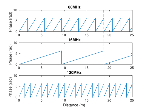
Figure 2 shows the phase to distance relation for the three amplitude-modul-ated signals, with frequencies 16, 80 and 120 MHz, which is the setup used in the Kinect v2 [2]. For each of the three frequencies, three phase shifts are used to calculate a phase according to (2), and thus a total of nine measurements are used in each depth calculation. In the figure, we see that if the phase shifts are combined, a common wrap-around occurs at 18.75 meters. This is thus the maximum range in which the Kinect v2 can operate without depth ambiguity.
As a final step, the phase shifts from the different modulation frequencies are combined using a phase unwrapping procedure and a weighted average.
It is of critical importance that the phase is correctly unwrapped, as choosing the wrong period will result in large depth errors. This is the topic of the following sub-sections.
2.1 Phase unwrapping
Consider phase measurements of amplitude modulated signals with different modulation frequencies. From (3) we get the following relations:
| (5) | |||
| (6) |
where are the least common multiples for divided by the respective frequency and are the set of sought unwrapping coefficients. Now (6) can be simplified to a set of constraints on pairs of unwrapping coefficients :
| (7) |
In total there are such equations. As the system is redundant, the correct unwrapping cannot be obtained by e.g. Gaussian elimination and in practice the equations are unlikely to hold due to measurement noise. The constraints can however be used to define a likelihood for a specific unwrapping.
2.2 CRT based unwrapping
The ambiguity of the phase measurements can be resolved by applying a variant of the Chinese reminder theorem (CRT) [4, 5] to one equation at a time in (7):
| (8) | ||||
| (9) |
In the case of more than two frequencies the unwrapped phase could be used in (8) for the next equation in (7) to unwrap the next phase. This is suggested and described in [5] and is also used in libfreenect2. In the end when all equations have been used, the full unambiguous range of the combined phase measurements has been unwrapped. The CRT method is fast but sensitive to noise as it unwraps each of the phase measurements in sequence. The consequence of this is that an error made early on will be propagated.
2.3 Phase fusion
The unwrapped phase measurements are combined by using a weighted average:
| (10) |
where is the standard deviation of the noise in . The pseudo distance estimate is later converted to a depth (i.e. distance in the forward direction), using the intrinsic camera parameters.
3 Kernel Density based Unwrapping
In this paper, we propose a new method for multi-frequency phase unwrapping. The method considers several fused pseudo distances (see (10)) for each pixel location , and select the one with the highest kernel density value [16]. Each such hypothesis is a function of the unwrapping coefficients . The kernel density for a particular hypothesis is a weighted sum of all considered hypotheses in the spatial neighbourhood:
| (11) |
Here is the kernel, and is a sample weight. The sets of samples to consider are defined by the hypothesis indices (e.g. if we have two hypotheses in each pixel), and by the set of all spatial neighbours where is a square truncation radius. The hypothesis weight is defined as
| (12) |
The three factors in are:
-
•
the spatial weight , which is a Gaussian that downweights neighbours far from the considered pixel location .
-
•
the unwrapping likelihood , that depends on the consistency of the pseudo-distance estimate (10) given the unwrapping vector
. -
•
the phase likelihood , where , are the amplitudes from (2). It defines the accuracy of the phase before unwrapping.
The kernel in (11) is defined as:
| (13) |
where is the kernel scale.
In the following sub-sections we will describe the three weight terms in more detail. For simplicity of notation, we will drop the pixel coordinate argument , and e.g. write instead of .
3.1 Unwrapping likelihood
Due to measurement noise, the constraints in (7) are never perfectly satisfied. We thus subtract the left-hand side from the right-hand side of these equations to form residuals , one for each of the constraints. These are then used to define a cost for a given unwrapping vector :
| (14) |
This cost function corresponds to the following unwrapping likelihood:
| (15) |
where is the fusion of the three unwrapped pseudo-distances, see (10), and is a scaling factor to be determined. For normally distributed residuals, and the Kinect v2 case of , the constraints in (7) imply:
| (16) | ||||
| (17) | ||||
| (18) |
This gives us the weights in (14). The values of could be predicted from the phase amplitude (more on this later), but they tend to deviate around a fixed ratio, and we have observed better robustness of (15) if the ratio is always fixed. We assume that the phase variances is equal for all modulation frequencies. This assumption gives us their relative magnitudes, but not their absolute values, which motivates the introduction of the parameter in (15).
3.2 Multiple hypotheses
In contrast to the CRT approach to unwrapping, see section 2.2, we will consider all meaningful unwrapping vectors within the unambiguous range. A particular depth value corresponds to a unique unwrapping vector, but with the introduction of noise, neigbouring unwrappings need to be considered at wrap around points. For example, looking at the Kinect v2 case shown in figure 2, if , should either be 0 or 1. In total different hypotheses for are constructed in this way. These can then be ranked by (15).
Compared with the CRT approach, that only considers one hypothesis, the above approach is more expensive. On the other hand, the true maximum of (15) is guaranteed to be checked.
In the low noise case, we can expect the hypothesis with the largest likelihood according to (15) to be the correct one. This is however not necessarily the case in general. Therefore a subset of hypotheses with high likelihoods are saved for further consideration, by evaluating the full kernel density (11).
3.3 Phase likelihood
The amplitude, , produced by (2) can be used to accurately propagate a noise estimate on the voltage values to noise in the phase estimate. In [13] this relationship is analysed and an expression is derived that can only be computed numerically. For practical use, [13] instead propose as approximate propagation formula (for ).
For constant but unknown noise variance on the voltage values , the phase noise can be predicted from the amplitude, as:
| (19) |
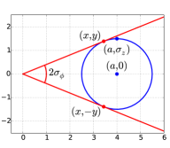
where is a parameter to be determined. While propagation of noise from voltage values to the complex phase vector is linear, the final phase extraction is not, and we will now derive a more accurate approximation using sigma-point propagation [17]. Geometrically, phase extraction from the phase vector (2) is a projection onto a circle, and thus the noise propagation is also a projection of the noise distribution onto the circle, see figure 4 (a). is centered around the true amplitude , and sigma-point candidates are located on a circle with radius . By finding the points where the circle tangents pass through the origin, we get an accurate projection of the noise distribution.
The points of tangency can be found using the pole-polar relationship [18]. For points and we get the expressions:
| (20) |
From these expressions, the phase noise can be predicted as:
| (21) |
where is a model parameter to be determined. Values of invalidate the geometric model in figure 4 (a), and for these we use (19) with .
In libfreenect2, a bilateral filter is applied to the vectors. The noise attenuation this results in is amplitude dependent, but it can be accurately modelled as a quadratic polynomial on .
| (22) |
We use the predicted phase noise to define a phase likelihood:
| (23) |
where is a parameter to be tuned. The phase likelihood encodes the accuracy of the phases before unwrapping.
3.4 Hypothesis selection
In each spatial position , we rank the considered hypotheses , using the KDE (kernel density estimate) defined in (11). The final hypothesis selection is then made as:
| (24) |
For the selected hypothesis, is also useful as a confidence measure that can be thresholded to suppress the output in problematic pixels. However, if the spatial support is small, e.g. , the weighted KDE occasionally encounters sample depletion problems (only very bad samples in a neighbourhood). This can be corrected by regularizing the confidence computation according to:
| (25) |
where is a small value, e.g. .
3.5 Spatial selection versus smoothing
The proposed KDE approach, see (11), selects the best phase unwrapping by considering the distribution of hypotheses in the spatial neighbourhood of a pixel. Note that the spatial neighbourhood is only used to select among different hypotheses. This is different from a spatial smoothing, as is commonly used in e.g. depth from disparity [19]. A connection to kernel based smoothing approaches, such as channel smoothing [20, 21] can be made by considering the limit where the number of hypotheses is the continuous set of -values in the depth range of the sensor. The discrete selection in (24) will then correspond to decoding of the highest peak of the PDF, and thus to channel smoothing. In the experiments we will however use just , or hypotheses per pixel, which is far from this limit. After selection, the noise on each pixel is still uncorrelated from the noise of its neighbours, and each pixel can thus still be considered an independent measurement. This is beneficial when fusing data in a later step, using e.g. Kinect Fusion [3].
4 Experiments
We apply the method to depth decoding for the Kinect v2 sensor, and compare it to the Microsoft Kinect SDK222Version 2.0.1409 in the following denoted Microsoft and to the open source driver libfreenect2. A first visual result is shown in figure 1. As can be seen in the figure, the proposed method has a better coverage in the depth images than libfreenect2. Another clear distinction between the methods is that libfreenect2 produces salt and pepper noise all over the image. See also [22] for more examples, and corresponding RGB frames.
4.1 Implementation
The algorithm was implemented by modifying the libfreenect2333As in Feb 18 2016 commit: 1d06d2db04a9 code for depth calculations using OpenCL [23] for GPU acceleration. When running the proposed pipeline with on a Nvidia GeForce GTX 760 GPU, the frame rate for the depth calculations is above 30 fps for spatial supports up to . For e.g. a support our method operates at 200 fps, which is marginally slower than libfreenect2 (which also operates in a neighbourhood) at fps. The current implementation is however designed for ease of testing, and further speed optimization is be possible.
| library(tuning) | kitchen(test) | lecture(test) |
 |
 |
|

|
 |
 |
4.2 Ground Truth for Unwrapping
We construct our own ground truth data, which is used for quantitatively evaluating the correctness of the phase unwrappings. The accuracy of the ground truth must be good enough to tell a correct unwrapping from an incorrect one. As we have 30 unwrapping candidates in an 18.75m range, the distance between the candidates is on average 60cm. To ensure that no incorrect unwrappings are accidentally counted as inliers, we require an accuracy of at least half the candidate distance, i.e. better than 30cm.
The required accuracy can easily be met using the Kinect sensor itself. By fusing many frames from the same camera pose, we can reduce the amount of unwrapping errors, and also increase the accuracy in correctly unwrapped measurements. For a given scene we place the camera at different locations corresponding to a spatial grid. By fusing data from these poses we can detect and suppress multipath responses, which vary with camera position. Further details on the dataset generation can be found in the supplemental materials [22].
4.3 Datasets
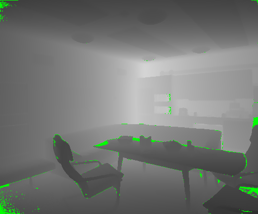
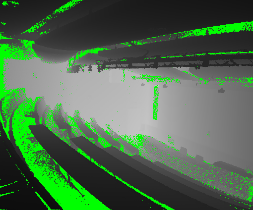
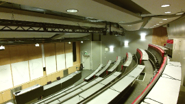
We have used the procedure in section 4.2 to collect three datasets with ground truth depth, shown in figure 3. The kitchen dataset has a maximal depth of m, and is used to test the Kinect v2 under the intended usage with an m depth limit. The lecture dataset has a maximal depth of m and is used to evaluate methods without imposing the m limit. The library dataset is used for parameter tuning, and has a maximal range of m. For each dataset, we have additionally logged raw-data frames from the central camera pose, using a data logger in Linux, and another output frames using the Microsoft SDK v2 API in Windows.
4.4 Comparison of noise propagation models
 |
 |
 |
| (a) | (b) | (c) |
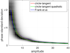
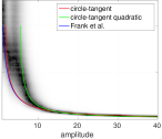
The tuning dataset library was used to estimate the standard deviations of the individual phase measurements over 40 frames. The model parameters in (19), (21) and (22) were found by minimizing the residuals of the corresponding inverted expressions using non-linear least squares over all amplitude measurements . The inversion of the expressions reduced bias effects due to large residuals for small amplitudes.
This procedure was performed for with and without bilateral filtering (as implemented in libfreenect2). Figure 4 ((b) and (c)) shows the resulting predictions overlaid on the empirical distributions of the relation between the amplitude and the phase standard deviation. We see that the models proposed in (21) and (22) have a slightly better fit to the empirical distribution than [13] on raw phase measurements. However, for bilateral filtered , the quadratic model suggested in expression (22) has the best fit. As bilateral filtering improves the final performance this is the model used in our method.
4.5 Outlier Rejection
libfreenect2: outlier rejection is performed at several steps, each with one or several tuned thresholds:
-
•
Pixels where any of the amplitudes is below a threshold are suppressed.
-
•
Pixels where the pseudo-distances differ in magnitude are suppressed. The purpose of this is similar to (15), but an expression based on the cross-product of the pseudo phases with a reference relation is used.
-
•
Pixels with a large depth, or amplitude variance in their neighbourhood are suppressed.
-
•
Pixels that deviate from their neighbours are suppressed.
-
•
Pixels on edges in the voltage images are suppressed.
Proposed method: a single threshold is applied on the KDE-based confidence measure in (25).
4.6 Parameter settings
The proposed method introduces the following parameters that needs to be set:
-
•
the scaling in (15)
-
•
the scaling in (23).
-
•
the kernel scale in (13).
-
•
the spatial support . (the Gaussian in (12) has a spatial support of and .)
-
•
the number of hypotheses .
The method is not sensitive to the selection of , and , and thus the same setting is used for all experiments. Unless otherwise stated, the parameters and are used. The effects of these parameters are discussed further in the supplemental material [22].
4.7 Coverage Experiments
| kitchen | kitchen (depth limited) | lecture |
|---|---|---|
 |
 |
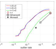 |
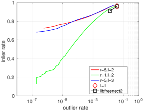
We have used the unwrapping datasets described in section 4.3 to compare the methods in terms of inliers (correctly unwrapped points), and outliers (incorrectly unwrapped points). A point is counted as an inlier when a method outputs a depth estimate which is closer than 30cm to the ground truth, and an outlier otherwise. These counts are then divided by the number of valid points in the ground truth to obtain inlier and outlier rates.
Figure 5 shows plots of inlier rate against outlier rate for our method, for the full range of thresholds on the output confidence in (25). As a reference, we also plot the output from Microsoft and libfreenect2, as well as libfreenect2 without the outlier threshold, and libfreenect2 where the hypothesis selection is done by minimising (14), instead of using the CRT approach in section 2.2 (labelled in the legend). As can be seen in figure 5 middle, the performance of libfreenect2 and Microsoft are similar on short range scenes with a depth limit (this is expected, as the libfreenect2 source mentions it being based on disassembly of the Microsoft SDK).
As can be seen, the proposed method consistently has a higher inlier rate at the same outlier rate, when compared to libfreenect2 with the same spatial support, i.e. . When the spatial support size is increased, the improvement is more pronounced.
Performance for scenes with larger depth is exemplified with the lecture dataset. With the depth limit removed, we get significantly more valid measurements at the same outlier rate. The Microsoft method has a hard limit of m and cannot really compete on this dataset; it only reaches about inlier rate. The libfreenect2 method without the depth limit reaches inliers, at a outlier rate. At the outlier rate, the proposed method has a inlier rate, which is an relative improvement of over libfreenect2.
The performance is improved slightly for compared with . While still having frame rates over 30 fps for a spatial support of , we consider the costs to outweigh the small improvement, and thus favour the setting of .
4.8 Kinect Fusion
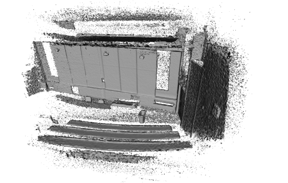
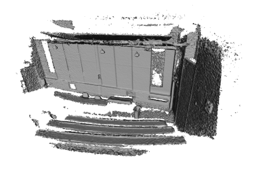
We have implemented a data-logger that saves all output from the Kinect v2 to a file for later playback. This allows us to feed the Kinect Fusion implementation KinFu in the Point Cloud Library [24] with Kinect v2 output unwrapped with both libfreenect2 and the proposed method. Figure 6 shows two meshes obtained in this way. As can be seen Kinect Fusion benefits from the proposed approach by generating models with fewer outlier points, and consistently more complete scene details. See [22] for more examples.
5 Concluding Remarks
This paper introduces a new multi-frequency phase unwrapping method based on kernel density estimation of phase hypotheses in a spatial neighbourhood. We also derive a new closed-form expression for prediction of phase noise and show how to utilize it as a measure of confidence for the measurements.
Our method was implemented and tested extensively on the Kinect v2 time-of-flight depth sensor. Compared to the previous methods in libfreenect2 and Microsoft Kinect SDK v2 it consistently produces more valid measurements when using the default depth limit of m, while maintaining real-time performance. In large-depth environments, without the depth limit, the gains are however much larger, and the number of valid measurements increases by at the same outlier rate.
As we have shown, the proposed method allows better 3D scanning of large scenes, as the full m depth range can be used. This is of interest for mapping and robotic navigation, where seeing further allows better planning. As the method is generic, future work includes applying it to other multi-frequency problems such as Doppler radar [1] and fringing [5, 6].
5.0.1 Acknowledgements
This work has been supported by the Swedish Research Council in projects 2014-6227 (EMC2) and 2014-5928 (LCMM) and the EU’s Horizon 2020 Programme grant No 644839 (CENTAURO).
References
- [1] Trunk, G., Brockett, S.: Range and velocity ambiguity resolution. In: IEEE National Radar Conference. (1993) 146–149
- [2] Sell, J., O’Connor, P.: The Xbox One system on a chip and Kinect sensor. IEEE Micro 34(2) (March-April 2014)
- [3] Newcombe et al., R.A.: KinectFusion: Real-time dense surface mapping and tracking. In: IEEE ISMAR’11, Basel, Switzerland (October 2011)
- [4] Jongenelen, A.P.P., Bailey, D.G., Payne, A.D., Dorrington, A.A., Carnegie, D.A.: Analysis of errors in tof range imaging with dual-frequency modulation. IEEE transactions on instrumentation and measurement 60(5) (May 2011)
- [5] Wang, Z., Du, H., Park, S., Xie, H.: Three-dimensional shape measurement with a fast and accurate approach. Applied optics 48(6) (2009) 1052–1061
- [6] Gorthi, S.S., Pastogi, P.: Fringe projection techniques: Wither we are? Optics and Lasers in Engineering 48(2) (2010) 133–140
- [7] Hansard, M.: Chapter 2: Disambiguation of time-of-flight data. In: Time-of-Flight Cameras, Springer Briefs in Computer Science. (2013)
- [8] Crabb, R., Manduchi, R.: Fast single-frequenct time-of-flight range imaging. In: IEEE International Conference on Computer Vision and Pattern Recognition (CVPR’15). (2015)
- [9] Droeschel, D., Holz, D., Behnke, S.: Multi-frequency phase unwrapping for time-of-flight cameras. In: IEEE International Conference on Intelligent Robots and Systems. (2010)
- [10] Kirmani, A., Benedetti, A., Chou, P.A.: SPUMIC: Simultaneous phase unwrapping and multipath interference cancellation in time-of-flight cameras using spectral methods. In: IEEE International Conference on Multimedia & Expo (ICME’13). (2013)
- [11] Feigin, M., Bhandari, A., Izadi, S., Rhemann, C., Schmidt, M., Raskar, R.: Resolving multipath interference in Kinect: An inverse problem approach. IEEE Sensors Journal (2015) Accepted, On-line.
- [12] Mei, J., Kirmani, A., Colaco, A., Goyal, V.K.: Phase unwrapping and denoising for time-of-flight imaging using generalized approximate message passing. In: IEEE International Conference on Image Processing (ICIP’13). (2013)
- [13] Frank, M., Plaue, M., Rapp, H., Köthe, U., Jähne, B.: Theoretical and experimental error analysis of continuous-wave time-of-flight range cameras. Optical Engineering 48(1) (January 2009)
- [14] Bamji, C., Charbon, E.: US 6,515,740 B2: Methods for CMOS-compatible three-dimensional image sensing using quantum efficiency modulation (2004)
- [15] Bamji et al., C.S.: A 0.13 m CMOS system-on-chip for a time-of-flight image sensor with multi-frequency photo-demodulation up to 130 MHz and 2 GS/s ADC. IEEE Journal on Solid-State Circuits 50(1) (January 2015)
- [16] Murphy, K.P.: Machine Learning: A Probabilistic Perspective. MIT Press (2012)
- [17] Uhlmann, J.: Dynamic Map Building and Localization: New Theoretical Foundations. PhD thesis, University of Oxford (1995)
- [18] Hartley, R., Zisserman, A.: Multiple View Geometry in Computer Vision. 2nd edn. Cambridge University Press (2003)
- [19] Szeliski, R.: Computer Vision: Algorithms and Applications. Springer-Verlag New York, Inc. (2010)
- [20] Forssén, P.E.: Low and Medium Level Vision using Channel Representations. PhD thesis, Linköping University, Sweden, SE-581 83 Linköping, Sweden (March 2004) Dissertation No. 858, ISBN 91-7373-876-X.
- [21] Felsberg, M., Forssén, P.E., Scharr, H.: Channel smoothing: Efficient robust smoothing of low-level signal features. IEEE TPAMI 28(2) (February 2006) 209–222
- [22] Anonymous: Efficient multi-frequency phase unwrapping using kernel density estimation, supplemental material. Technical report, A Department (2016)
- [23] Khronos Group: OpenCL language specification. https://www.khronos.org/opencl/ (2015)
- [24] Rusu, R.B., Cousins, S.: 3D is here: Point Cloud Library (PCL). In: IEEE ICRA. (May 9-13 2011)