The probability of nonexistence of a subgraph in a moderately sparse random graph

Abstract

We develop a general procedure that finds recursions for statistics counting isomorphic copies of a graph $G_{0}$ in the common random graph models ${\cal G}(n,m)$ and ${\cal G}(n,p)$. Our results apply when the average degrees of the random graphs are below the threshold at which each edge is included in a copy of $G_{0}$. This extends an argument given earlier by the second author for $G_{0}=K_{3}$ with a more restricted range of average degree. For all strictly balanced subgraphs $G_{0}$, our results give much information on the distribution of the number of copies of $G_{0}$ that are not in large “clusters” of copies. The probability that a random graph in ${\cal G}(n,p)$ has no copies of $G_{0}$ is shown to be given asymptotically by the exponential of a power series in $n$ and $p$, over a fairly wide range of $p$. A corresponding result is also given for ${\cal G}(n,m)$, which gives an asymptotic formula for the number of graphs with $n$ vertices, $m$ edges and no copies of $G_{0}$, for the applicable range of $m$. An example is given, computing the asymptotic probability that a random graph has no triangles for $p=o(n^{-7/11})$ in ${\cal G}(n,p)$ and for $m=o(n^{15/11})$ in ${\cal G}(n,m)$, extending results of the second author.

1 Introduction

Our topic is the number of subgraphs of a random graph that are isomorphic to some given graph $G_{0}$. The perturbation method of [11] is used to derive recursions of ratios of random graph statistics describing the occurence of different types of clusters formed as edge-overlapping groups of copies of $G_{0}$. These recursions are used to investigate the probability of no occurrences of $G_{0}$, as well as other aspects of the distribution of clusters. For certain graphs $G_{0}$ and restrictions on $p$, we show that the probability that there are no copies of the graph in ${\cal G}(n,p)$ is the exponential an appropriate truncation of a power series in $n$ and $p$, with error factor $(1+o(1))$. (As is usual, ${\cal G}(n,p)$ denotes the random graph on $n$ vertices obtained by choosing each edge in the graph to be present independently with probability $p$ and ${\cal G}(n,m)$ denotes the random graph on $n$ vertices obtained by choosing uniformly at random from the $\binom{\binom{n}{2}}{m}$ graphs having $m$ edges.) By considering recursions involving both $G_{0}$ and isolated edges, we build on this result to show that the probability that there are no copies of $G_{0}$ in ${\cal G}(n,m)$ is given in the same way but by a different power series in $n$ and $d$, where

$$d=\frac{m}{\binom{n}{2}},$$ (1.1)

under corresponding restrictions on $d$.

Let $\nu(G)$ and $\mu(G)$ denote the number of vertices and number of edges of a graph $G$. A graph $G_{0}$ is strictly balanced if all its subgraphs are strictly less dense than $G_{0}$; that is,

$$\frac{\mu(G_{0})}{\nu(G_{0})}>\frac{\mu(G_{1})}{\nu(G_{1})}$$

for all nontrivial proper subgraphs $G_{1}$ of $G_{0}$. For example, the graph $K_{n}$ is strictly balanced for all $n\geq 2$, as is every cycle. Let $G_{0}$ be strictly balanced, and let $X$ be the number of copies of $G_{0}$ in the random graph ${\cal G}(n,p)$. Let $\chi>0$ be defined by

$$\chi=\chi(G_{0})=\max_{G_{1}\in{\cal E}}\frac{\nu(G_{0})-\nu(G_{1})}{\mu(G_{0})-\mu(G_{1})}.$$ (1.2)

We will restrict the growth of $p$ to $p=O(n^{-\chi-\epsilon})$ for some $\epsilon>0$. The reason for this restriction is that when $p$ is a little larger than $n^{-\chi}$ (sometimes called the 2-threshold), each edge of ${\cal G}(n,p)$ will expect to be contained in many copies of $G_{0}$. Thus, there will be subgraphs consisting of arbitrarily large numbers of copies of $G_{0}$ “chained” together by shared edges. In this case our analysis will not apply, since it relies on a copy of $G_{0}$ being unlikely to overlap with any others, as happens when restricting to $p=O(n^{-\chi-\epsilon})$.

Here is our main result. Note that $\chi$ should not be confused with the chromatic number, which does not appear in this paper.

Theorem 1.1

Let $G_{0}$ be strictly balanced and put $\chi=\chi(G)$. Let $X$ be the number of copies of $G_{0}$ in ${\cal G}(n,p)$, or let $X$ be the number of copies of $G_{0}$ in ${\cal G}(n,m)$ and set $p=m/\binom{n}{2}$. In each case, there is a formal power series $F=F(G_{0})=\sum_{\ell\geq 0}c_{\ell}n^{i_{\ell}}p^{j_{\ell}}$, with $i_{\ell}$ and $j_{\ell}$ strictly positive for all $\ell$, depending only on $G_{0}$, such that the following holds. For any $\epsilon>0$, if $p=O(n^{-\chi-\epsilon})$, then

$${\bf P}(X=0)=\exp\left(\sum_{\ell=0}^{M_{\epsilon}}c_{\ell}n^{i_{\ell}}p^{j_{\ell}}+o(1)\right),$$ (1.3)

where the bound implicit in $o(1)$ is uniform over all such $p$ (but depends on $\epsilon$), and $M_{\epsilon}$ is a constant depending only on $\epsilon$ and $G_{0}$. Moreover, $\ell>M_{\epsilon}$ if and only if $i_{\ell}<j_{\ell}(\chi+\epsilon)$.

Remarks

1. The theorem immediately gives an asymptotic formula for the number of $G_{0}$-free graphs on $n$ vertices and $m$ edges, for the values of $m$ covered, by multiplying the ${\cal G}(n,m)$ case of (1.3) by ${n(n-1)/2\choose m}$.

2. Note that $i_{\ell}<j_{\ell}(\chi+\epsilon)$ if and only if $n^{i_{\ell}}p^{j_{\ell}}=o(1)$ when $p=n^{-\chi-\epsilon}$, so each term with $\ell>M_{\epsilon}$ is $o(1)$. We also note that the issue of non-convergence of the power series $F(G_{0})$ for a given fixed $n$ and $p$ is not relevant in the present context.

3. The proof of the theorem contains a definition of the coefficients $c_{\ell}$ in Theorem 1.1 in terms of an algorithm by which they may be computed. It involves summing over a set of graphs whose size is bounded for fixed $\epsilon>0$, but not as $\epsilon\to 0$.

We next give two specific examples of the main result, by restricting to that case that $G_{0}$ is a triangle, or $K_{3}$, and computing only the first few terms of the power series explicitly.

Theorem 1.2

If $p=p(n)=o(n^{-7/11})$, the probability that the random graph ${\cal G}(n,p)$ is triangle-free is asymptotic to

$$\exp\left(-\frac{1}{6}n^{3}p^{3}+\frac{1}{4}n^{4}p^{5}-\frac{7}{12}n^{5}p^{7}+\frac{1}{2}n^{2}p^{3}-\frac{3}{8}n^{4}p^{6}+\frac{27}{16}n^{6}p^{9}\right).$$

Similarly, we determine the coefficients $c_{\ell}$ in the case of ${\cal G}(n,m)$ where $G_{0}=K_{3}$ and $d=o(n^{-7/11})$, or equivalently $m=o(n^{15/11})$, in the next theorem.

Theorem 1.3

If $m=m(n)=o(n^{15/11})$, the probability that the random graph ${\cal G}(n,m)$ is triangle-free is asymptotic to

$$\exp\left(-\frac{1}{6}n^{3}d^{3}-\frac{1}{8}n^{4}d^{6}\right),$$

where $d=m/\binom{n}{2}$.

These two results on triangles agree with and extend those of the second author in [11], which applied for $p=o(n^{-2/3})$ and extended earlier results of Frieze [3].

For ${\cal G}(n,m)$, the expected value of $X$ is easily found to be

$$\lambda(G_{0}) := \binom{n}{\nu}\binom{m}{\mu}\binom{\binom{n}{2}}{\mu}^{-1}\nu!|\mbox{aut}(G_{0})|^{-1}$$

$$\sim \hat{\lambda}(G_{0}):=\frac{(2m)^{\mu}}{n^{2\mu-\nu}|\mbox{aut}(G_{0})|}$$

where $\nu=\nu(G_{0})$, $\mu=\mu(G_{0})$, and $|\mbox{aut}(G_{0})|$ denotes the number of automorphisms of $G_{0}$. Ruciński [10] showed that the distibution of $X$ is asymptotically Poisson essentially for $d$ up to $n^{-\chi}$. Frieze [3, Remark 2, P.69] raised the possibility that, for the same range of $d$, the number of graphs with $k$ copies of $G_{0}$ in ${\cal G}(n,m)$ is asymptotic to the probability that the Posson random variable with mean $\hat{\lambda}(G_{0})$ is equal to $k$, for all “small” $k$. Theorem 1.3 shows (for the first time!) that this is false in particular for $k=0$ and $G_{0}=K_{3}$, since in this case, $\chi=1/2$ but already for $m=n^{4/3}$, other terms are entering the asymptotic formula in a significant way. Moreover, the situation is not remedied by using (the more natural) Poisson with mean $\lambda(G_{0})$, since $\lambda(G_{0})=\frac{1}{6}n^{3}d^{3}-\frac{1}{2}n^{2}d^{3}+o(1)$ (using $nd^{2}=O(m^{2}/n^{3})=o(1)$ for the range of $m$ under consideration).

We note that it may be possible to modify our approach to cater also for subgraphs that are not strictly balanced. In some cases, for instance where $G_{0}$ has a unique densest subgraph, the desired result can be deduced immediately from our results. However, other cases are more delicate, with different subgraphs of $G_{0}$ ‘competing’. One would need to incorporate considerations similar to those in the determination the threshold of appearance of $G_{0}$, as was done by Bollobás [1].

Our concern here is to obtain an asymptotic formula for the probability that a random graph in ${\cal G}(n,p)$ or ${\cal G}(n,m)$ is $G_{0}$-free, for a fixed graph $G_{0}$, where the density of the random graph is small enough that there are no large clusters of copies of $G_{0}$. Our methods will not work for the denser case, but some results are already known there, and for arbitrary densities. Recall, as in Remark 2 above, that for ${\cal G}(n,m)$ our problem is equivalent to enumerating $m$-edged graphs with a forbidden subgraph. The classic paper of Erdős, Kleitman and Rothschild [2] gives the number of triangle-free graphs with $n$ vertices, in total, asymptotically (and asymptotics of the logarithm of the number when $G_{0}=K_{t}$). These results also demonstrate the connection between enumeration and the extremal numbers of edges for $G_{0}$-free graphs. There are many other similar results, which we refrain from mentioning as they do not take into accoung the edge density of the host graph. More related to the problem at hand, Prömel and Steger [9] found an asymptotic formula for the number of triangle-free graphs with $n$ vertices and $m$ edges when $m>cn^{7/4}\log n$, by showing that they are almost all bipartite. This was extended by D. Osthus, H.J. Prömel and A. Taraz [7] to cover all $m$ that are at least slightly above $n^{3/2}$. Before this, Łuczak [6] had found asymptotics of the logarithm of the number.

For more general subgraphs than the triangle, and general $p$, asymptotic formulae for the actual numbers (or probabilities) are elusive. The logarithm of the probability that ${\cal G}(n,p)$ is $G_{0}$-free was estimated within a constant factor by Janson, Łuczak and Ruciński [4]. This was extended by Prömel and Steger [8] to similar bounds on ${\bf P}\big{(}\mbox{${\cal G}(n,m)$ is $G_{0}$-free}\big{)}$.

Many results are known on the distribution of the number of copies of a fixed subgraph in ${\cal G}(n,p)$ and ${\cal G}(n,m)$; see for example [5, Chapter 6], but this is not our concern in this paper.

Our basic approach, and its background, are discussed in [11]. The proof for ${\cal G}(n,p)$ estimates ratios of numbers of graphs using induction on the numbers of edge-overlapping clusters of copies of $G_{0}$ up to a given size; for ${\cal G}(n,m)$ the number of edges not in copies of $G_{0}$ is also used, and the base step of this induction is essentially given by the $n$-vertex graph with no edges. There are two major extensions to the argument in [11]. One is that the graph $G_{0}$ is no longer restricted to $K_{3}$. This extension requires mainly graph theoretic arguments related to the ways that multiple copies of a graph can overlap. The other is that the range of $p$ permits edge-overlapping clusters containing arbitrarily many copies of $G_{0}$ to appear in the typical random graph under consideration. Thus our asymptotic estimates involve polynomials of unbounded size, and this poses significant problems in characterising and managing those estimates (see Corollary 2.7 for example).

The working assumption on $p=p(n)$ we will make in our proofs is $p=n^{-\kappa+o(1)}$ where $\kappa\geq\chi+\epsilon$ is fixed. This assumption can be weakened to obtain asymptotic results that hold uniformly over more general $p=p(n)=O(n^{-\chi-\epsilon})$ by using the following lemma. Here $a$ and $b$ are finite but the same result holds (with appropriate interpretation) without this assumption.

Lemma 1.4

For a closed interval $[a,b]$, suppose that $f(n,p)$ is a function such that $f(n,p)\to 0$ as $n\to\infty$ for all $p$ of the form $p=n^{-\kappa+o(1)}$ when $\kappa\in[a,b]$ is fixed. Then for fixed $\epsilon>0$, $f(n,p)\to 0$ uniformly for all $p(n)$ satisfying $p(n)=n^{-\kappa(n)}$ with $\kappa(n)\in[a,b]$ for all $n$.

Proof. If $p(n)$ satisfies $-\log_{n}p\in[a,b]$ for all $n$, then any subsequence of $\big{(}p(n)\big{)}_{n\geq 1}$ has a subsubsequence for which $-\log_{n}p\to\kappa^{\prime}$ for some fixed $\kappa^{\prime}\in[a,b]$. On this subsubsequence, $f(n,p)\to 0$ by assumption. So the lemma follows from the subsubsequence principle (see [5, p.12]) applied to the sequence $\big{(}f(n,p(n))\big{)}_{n\geq 1}$ .   

Our results will give information on the distribution of the number of copies of a strictly balanced subgraph, not just the probability that the number is 0, but we postpone this investigation to another paper. We believe that it should be possible to modify our approach so as to obtain accuracy in the formulae to any desired power of $n^{-{1}}$. Specifically, the power series in Theorem 1.1 should give valid lower order correction terms to the asymptotic formulae. However, we have avoided attempting this and there are some steps in the present argument that would have to be replaced in order to carry it out.

Some basic definitions are made and results are proved in Section 2; the ${\cal G}(n,p)$ case of Theorem 1.1 is proved in in Section 3; the ${\cal G}(n,m)$ case is proved in in Section 4; Theorems 1.2 and 1.3 are proved in Appendix A.

2 Clusters and recursions for counting maximal clusters

We assume for a general framework that $\Omega$ is any finite set. A family ${\cal K}$ of subsets of $\Omega$ is called a clustering if $C_{1}\in{\cal K}$, $C_{2}\in{\cal K}$ and $C_{1}\cap C_{2}\neq\emptyset$ imply that $C_{1}\cup C_{2}\in{\cal K}$. The elements of ${\cal K}$ are called clusters.

We will consider here only the case that $\Omega=\Omega_{n}$ is the set of edges of the complete graph $K_{n}$ on $n$ vertices, although the same principles can also be applied to clusterings in general. As a further restriction, to focus on small subgraph counts, we only consider very special clusterings, for which simplification occurs by taking advantage of the symmetries of $K_{n}$. We take a fixed graph $G_{0}$ throughout this paper, and will investigate the distribution of the number of subgraphs of a random graph isomorphic to $G_{0}$. The edge set of any subgraph of $K_{n}$ isomorphic to $G_{0}$ is called an elementary $G_{0}$-cluster. Mostly, we deal with the minimal clustering which has every elementary $G_{0}$-cluster as a member. We call this the $G_{0}$-clustering of $\Omega$. Equivalently, $J\subseteq\Omega$ is in the $G_{0}$-clustering if and only if there is a sequence $J_{1},\ldots,J_{i}$ of subsets of $\Omega$ such that each $J_{j}$ is an elementary $G_{0}$-cluster, $\bigcup_{j=1}^{i}J_{j}=J$, and $J_{k}\cap\bigcup_{i=1}^{k-1}J_{j}\neq\emptyset$ for $2\leq k\leq i$. (This definition of clusters corrects an error in the definition in [11]. The usage of it in [11] is consistent with the present definition.)

More generally, suppose ${\cal R}$ is any fixed set of nonempty graphs, and information is desired on the joint distribution of the subgraph counts for the graphs in ${\cal R}$. Then the appropriate clustering to consider is the minimal clustering containing every elementary $G$-cluster for every $G\in{\cal R}$. We call this the clustering generated by ${\cal R}$. Of course, if ${\cal R}=\{G_{0}\}$, this is simply the $G_{0}$-clustering.

Henceforth in this paper we consider the clustering generated by a fixed set of graphs ${\cal R}$, and assume that each graph in ${\cal R}$ has no isolated vertices. Our first proposition considers a general set ${\cal R}$, and after that we restrict to only two kinds of clustering: the $G_{0}$-clustering, and the one generated by ${\cal R}=\{G_{0},K_{2}\}$, which we call the $G_{0}^{*}$-clustering. Note that a 1-element subset of $\Omega$ cannot have a nontrivial proper intersection with any other cluster. It follows that the $G_{0}^{*}$-clustering consists of the clusters of the $G_{0}$-clustering, together with all the 1-element subsets of $\Omega$. We assume in all cases that $|E(G_{0})|\geq 2$.

For $H\subseteq\Omega$, a cluster of $H$ is any cluster in ${\cal K}$ contained in $H$. A maximal cluster $Q$ of $H$ is cluster of $H$ which is contained in no larger cluster of $H$. Equivalently, $Q$ is a subset of $H$ such that $Q\in{\cal K}$ and such that for every $J\in{\cal K}$ with $J\subseteq H$, either $J\subseteq Q$ or $J\cap Q=\emptyset$. (The case of nonempty intersection is excluded by the definition of a clustering.) For example, if ${\cal K}$ is the $G_{0}$-clustering and $H$ is an arbitrary subset of $\Omega)$, a maximal cluster of $H$ whose cardinality is $|E(G_{0})|$ must be an elementary $G_{0}$-cluster contained in $H$ having empty intersection with every other elementary $G_{0}$-cluster in $H$.

Being a subset of $\Omega$, a cluster induces a subgraph of $K_{n}$. The isomorphism class of the subgraph is called the type of the cluster and also of the subgraph. The set of types will be denoted ${\cal T}$, and we use $\tau$ to denote the function which maps a cluster or the corresponding graph to its type. Given $t\in{\cal T}$, we use the notation $|t|:=|\{S\subseteq\Omega:\tau(S)=t\}|$. Note that this depends on $n$, whereas $t$ is fixed.

We will define a special nonempty finite set ${\cal S}$ of types which is closed under taking subsets, i.e. which satisfies

$$\mbox{if $S$, $S^{\prime}\in{\cal K}$, $\tau(S)\in{\cal S}$ and $S^{\prime}\subseteq S$ then $\tau(S^{\prime})\in{\cal S}$}.$$

Let $s=|{\cal S}|$ be the number of types in ${\cal S}$.

The types in ${\cal S}$ will be called small, and any cluster $Q$ with $\tau(Q)\in{\cal S}$ is also called small. Any type or cluster which is not small is called large. An unavoidable cluster is any large cluster which is a union of a small cluster $Q$ and a set of small clusters all pairwise disjoint and all having nonempty intersection with $Q$. The set of types of unavoidable clusters is denoted by ${\cal U}$. (The term “unavoidable” refers to the fact that large clusters created in a certain way, to be specified later, cannot avoid being in ${\cal U}$.)

We will need to record how many subgraphs of every small type are present in a given graph. So we consider the set ${\cal F}$ of all non-negative integer functions defined on ${\cal S}$. For any $H\subseteq\Omega$, define $s_{H}$ to be the function in ${\cal F}$ such that, for all $t\in{\cal S}$, $s_{H}(t)$ is the number of maximal clusters of $H$ of type $t$. The function $\delta_{t}\in{\cal F}$ has value 1 at $t$ and 0 elsewhere.

All our basic work is in ${\cal G}(n,p)$, the standard edge-independent (binomial) model for random graphs, and ${\bf P}$ and ${\bf E}$ denote probability and expectation in this space. $G$ denotes a random graph in ${\cal G}(n,p)$ and $q$ always denotes $1-p$. For $H\subseteq\Omega$, the event $H\subseteq E(G)$ is denoted by $A_{H}$, so that ${\bf P}(A_{H})=p^{|H|}$. The main objects we work with are, for each $f\in{\cal F}$, the set ${\cal C}_{f}$ consisting of graphs $G$ on $n$ vertices containing no large clusters and such that $s_{E(G)}=f$. For $f\notin{\cal F}$, for example if $f$ has a negative value on ${\cal S}$, we define ${\cal C}_{f}=\emptyset$. We write ${\bf P}({\cal C}_{f})$ for ${\bf P}({\cal G}(n,p)\in{\cal C}_{f})$.

For types $u,t\in{\cal S}$ and for $h\in{\cal F}$, define, for any fixed cluster $J$ of type $u$,

$$c(u,t,h)=\sum_{{Q\in{\cal K}\atop Q\subseteq J}\atop\tau(Q)=t}\sum_{H\cup Q=J\atop{s_{H}=h}}p^{|Q\cap H|}q^{|J\setminus H|}.$$ (2.1)

Since the clustering generated by any set ${\cal R}$ is symmetrical, $c(u,t,h)$ is clearly independent of the choice of $J$ with $\tau(J)=u$. Note that in the special case $u=t$,

$$c(t,t,h)=\sum_{H\subseteq J\atop{s_{H}=h}}p^{|H|}q^{|J\setminus H|},$$ (2.2)

and in particular

$$c(t,t,{\bf 0})=1+O(p).$$ (2.3)

We use $\nu(G)$ and $\mu(G)$ for the numbers of vertices and edges of a graph $G$ respectively, and extend the notation to arbitrary subsets $H$ of $\Omega$, so that $\nu(H)$ is the number of vertices of the graph induced by $H$ and $\mu(H)$ is the number of edges. In particular, this applies to clusters $H$. We also use $\nu(t)$ for the number of vertices in each cluster of type $t$ and $\mu(t)$ for the number of edges.

Let $[n]_{k}$ denote $n(n-1)\cdots(n-k+1)$. For $t\in{\cal T}$, let $Q$ be any cluster of type $t$ and $|\mbox{aut}(Q)|$ the number of automorphisms of the graph induced by $Q$. Then

$$|t|=\frac{[n]_{\nu(Q)}}{|\mbox{aut}(Q)|},$$ (2.4)

and

$$\lambda_{t}:=|t|p^{\mu(Q)}=\Theta(n^{\nu(Q)}p^{\mu(Q)})$$ (2.5)

is the expected number of different copies, in $G\in{\cal G}(n,p)$, of the subgraph induced by $Q$.

Our first result is obtained by simple counting.

Proposition 2.1

For $f\in{\cal F}$ and $t\in{\cal S}$,

$$\frac{{\bf P}({\cal C}_{f+\delta_{t}})}{{\bf P}({\cal C}_{f})}=\frac{\lambda_{t}}{(f(t)+1)c(t,t,{\bf 0})}\left(1-\Sigma-\frac{\theta(f,\delta_{t})}{|t|{\bf P}({\cal C}_{f})}\right)$$

where

$$\Sigma=\sum_{{u\in{\cal S}\atop h\in{\cal F}}\atop(u,h)\neq(t,{\bf 0})}\frac{(f(u)-h(u)+1)c(u,t,h){\bf P}({\cal C}_{f-h+\delta_{u}})}{\lambda_{t}{\bf P}({\cal C}_{f})}$$ (2.6)

and

$$0\leq\theta(f,\delta_{t})\leq\sum_{L\;:\>\tau(L)\in{\cal U}}\sum_{Q,H\subseteq L\atop{\tau(Q)=t\atop L\setminus Q\subseteq H}}{\bf P}({\cal C}_{f-s_{H}})\left(\frac{p}{q}\right)^{|H|}.$$ (2.7)

Proof. Note that

$$c(u,t,h)p^{-\mu(t)}=\sum_{{Q\in{\cal K}\atop Q\subseteq J}\atop\tau(Q)=t}\sum_{H\in{\cal C}_{h}\atop{H\cup Q=J}}\frac{q^{|J\setminus H|}}{p^{|Q\setminus H|}}=\sum_{{Q\in{\cal K}\atop Q\subseteq J}\atop\tau(Q)=t}\sum_{H\in{\cal C}_{h}\atop{H\cup Q=J}}\left(\frac{q}{p}\right)^{|J\setminus H|},$$

where we have used the fact that $J\setminus H=Q\setminus H$ follows from $H\cup Q=J$. Consider every pair $(E,Q)$ where $E$ is the edge set of a graph in ${\cal C}_{f}$ and $Q$ is a cluster of type $t$. Classifying $E\cup Q$ according to the type of its maximal cluster $L$ containing $Q$, and, in the case that $\tau(L)=u\in{\cal S}$, subclassifying according to $h=s_{E\cap L}$, gives

$$|t|{\bf P}({\cal C}_{f})=\Bigl{(}\sum_{u\in{\cal S}\atop h\in{\cal F}}(f(u)-h(u)+1)c(u,t,h)p^{-\mu(t)}{\bf P}({\cal C}_{f-h+\delta_{u}})\Bigr{)}+\theta(f,\delta_{t}),$$ (2.8)

where the $\theta$ term is bounded as in the statement of the proposition. This term comes from observing that if $L$ is a large cluster, then it must be unavoidable since $E$ has no large clusters, and from considering the subset of $\Omega$ obtained by removing the set $H$ of all edges of $E$ in $L$. Multiplying (2.8) by $p^{\mu(t)}$ gives

$$\lambda_{t}{\bf P}({\cal C}_{f})=\Bigl{(}\sum_{u\in{\cal S}\atop h\in{\cal F}}(f(u)-h(u)+1)c(u,t,h){\bf P}({\cal C}_{f-h+\delta_{u}})\Bigr{)}+\theta(f,\delta_{t})p^{\mu(t)}$$

and rearranging the terms, isolating the one with $(u,h)=(t,{\bf 0})$, finishes the proof.   

We now lay the groundwork for asymptotic results. Henceforth, we consider only the $G_{0}$- and $G_{0}^{*}$-clusterings for some fixed graph $G_{0}$ with at least two edges. Denote the set of proper subgraphs of $G_{0}$ which contain at least one edge by ${\cal E}$. Recalling that $|E(G_{0})|\geq 2$, we define the extension value of $G_{0}$ to be

$$x=x(G_{0},p,n)=\max_{G_{1}\in{\cal E}}\,n^{\nu(G_{0})-\nu(G_{1})}p^{\mu(G_{0})-\mu(G_{1})}.$$ (2.9)

For example, if $G_{0}$ is a triangle,

$$x=\max(np^{2},p,p^{2})=\max(np^{2},p).$$ (2.10)

The significance of the extension value lies in the fact that $n^{\nu(G_{0})-\nu(G_{1})}p^{\mu(G_{0})-\mu(G_{1})}$ is the asymptotically important part of

$${\left({n-\nu(G_{1})}\atop{\nu(G_{0})-\nu(G_{1})}\right)}p^{\mu(G_{0})-\mu(G_{1})}.$$

To interpret this quantity, first distinguish one of the subgraphs of $G_{0}$ isomorphic to $G_{1}$. For $G_{2}$ isomorphic to $G_{1}$, conditional upon $G_{2}\subseteq{\cal G}(n,p)$, the quantity above is the expected number of isomorphisms from $G_{0}$ to a subgraph of ${\cal G}(n,p)$ that map the distinguished copy of $G_{1}$ onto $G_{2}$.

For $H\subseteq E(K_{n})$ define $\Phi(H,G_{0})$ to be the expected number of subgraphs of $G\in{\cal G}(n,p)$ that are isomorphic to $G_{0}$ and whose edge set contains $H$, conditional on $H\subseteq E(G)$. Given a nonempty $H\subseteq\Omega$ which induces a proper subgraph of $G_{0}$, it follows from the remarks above that $\Phi(H,G_{0})$ is $O(x)$, since there is a bounded number of ways to distinguish one of the subgraphs of $G_{0}$ isomorphic to $G_{1}$.

Put a partial ordering on the set of types by defining $t$ to be strictly less than $u$ in the poset, denoted by $t\prec u$, if, and only if, any cluster of type $u$ properly contains a cluster of type $t$. If $t\prec u$, then a cluster of type $u$ can be obtained from a cluster $Q$ of type $t$ by a finite sequence of non-disjoint unions with clusters $Q_{0},\ldots,Q_{k}$ such that each $Q_{i}$ is the edge set of a graph isomorphic to some $G_{i}\in{\cal R}$ and $Q_{i}\not\subseteq Q\cup(\bigcup_{j=0}^{i-1}Q_{j})$. (Note that, in the $G_{0}^{*}$-clustering, it must be that $G_{i}=G_{0}$ for all $i$.) Thus, for $G\in{\cal G}(n,p)$ the expected number of clusters of type $u$ in $E(G)$ can be bounded above by a finite sum whose terms are all of the form $\lambda_{t}\prod_{i=0}^{k}\Phi(H_{i},G_{i})$ where $H_{i}$ corresponds to the intersection of $Q_{i}$ with $Q\cup(\bigcup_{j=0}^{i-1}Q_{j})$. Hence, from the conclusion of the previous paragraph, provided $x=o(1)$ we have

$$\mbox{if $t\prec u$ then }\frac{\lambda_{u}}{\lambda_{t}}=O(x).$$ (2.11)

Henceforth in this paper, we assume that $G_{0}$ is strictly balanced, with at least two edges. Let $X$ be the number of copies of $G_{0}$ in the random graph ${\cal G}(n,p)$. It follows easily from the definition (2.9) of $x$ that the constant $\chi$ defined in (1.2) is the smallest number such that $p=o(n^{-\chi})$ implies $x=o(1)$. Hence, there are functions $p=p(n)$ such that $\lambda_{\tau(G_{0})}\to\infty$ while $x(G_{0},p,n)=o(1)$. We also assume henceforth that $p=p(n)$ is restricted so that for some fixed $\kappa>\chi$,

$$p=n^{-\kappa+o(1)}.$$ (2.12)

This will be enough for our purposes in view of Lemma 1.4.

Fix $\epsilon>0$ and let $\kappa\geq\chi+\epsilon$. Since $\mu(G_{1})<\mu(G_{0})$ for all $G_{1}\in{\cal E}$, the expression maximised in (2.9) is at most $(n^{\chi}p)^{\mu(G_{0})-\mu(G_{1})}\leq n^{\chi}p$. Thus,

$$x(G_{0},p,n)=O(n^{-\epsilon+o(1)}).$$ (2.13)

See [5] for a general introduction to the considerations relevant here. Note that

$$p\leq x$$ (2.14)

by definition, as shown by setting the graph $G_{1}$ in (2.9) equal to $G_{0}$ minus an edge.

For our asymptotic results, we work with a particular set of small cluster types defined as follows:

$${\cal S}=\{t:\nu(t)/\mu(t)\geq\kappa\}.$$ (2.15)

Then for $t\in{\cal S}$, the expected number $\lambda_{t}$ of subgraphs of type $t$ is bounded below by $\lambda_{t}\geq n^{-o(1)}$ (here the negative sign is not necessary, just indicative, since $o()$ bounds the absolute value), since by (2.4), (2.5) and (2.12),

$$\lambda_{t}=\Theta(n^{\nu(t)-\kappa\mu(t)+o(1)}).$$ (2.16)

The set ${\cal S}$ is finite by (2.13) and (2.11). Hence, defining

$$\lambda_{\cal L}:=\sup_{t\notin{\cal S}}\lambda_{t}$$ (2.17)

we obtain

$$\lambda_{\cal L}=O(n^{-\epsilon^{\prime}})$$ (2.18)

for some $\epsilon^{\prime}>0$ by our definition of ${\cal S}$. While we are at it, due to a technicality we assume $\kappa<2$, so that $p$ satisfies the very weak growth condition

$$n^{2}p>n^{\epsilon^{\prime\prime}}$$ (2.19)

for some $\epsilon^{\prime\prime}>0$. This ensures that the number of edges in the random graph tends to infinity at a reasonable rate. Imposing this condition is without loss of generality, since the omitted case follows from the case considered. For example, the $p$ such that $p\sim n^{-c\nu(G_{0})/\mu(G_{0})}$ are covered for all $1<c<2\mu(G_{0})/\nu(G_{0})$, and this is well below the threshold of appearance of copies of $G_{0}$. Hence, each term in the power series must tend to zero for such $c$, and must also tend to 0 when $\kappa\geq 2$. The assumption $\kappa<2$ also ensures that, in the case of the $G_{0}^{*}$-clustering, the single edge cluster is in ${\cal S}$. Note that if $n^{2}p=o(\sqrt{n})$, the random graph is in any case not interesting, as it is asymptotically almost surely a matching.

Define

$${\cal S}_{0}=\{t\,:\,\nu(t)/\mu(t)=\kappa\},\quad{\cal S}_{1}={\cal S}\setminus{\cal S}_{0},$$

$$m_{t}=\left\{\begin{array}[]{ll}3\lambda_{t}&\mbox{ if }t\in{\cal S}_{1}\\ \lambda_{t}\log n&\mbox{ if }t\in{\cal S}_{0}.\end{array}\right.$$ (2.20)

Note that ${\cal S}_{0}$ will often be empty, but if it is nonempty, the types in ${\cal S}_{0}$ are the rarest types of small clusters in the random graph, and for $t\in{\cal S}_{0}$, we have $\lambda_{t}=n^{o(1)}$ and hence $m_{t}=n^{o(1)}$. Any type in ${\cal S}_{0}$ is maximal in ${\cal S}$ by (2.11). Thus, for later reference we may note that, for some positive $\epsilon^{\prime\prime\prime}$,

$$\lambda_{t}>n^{\epsilon^{\prime\prime\prime}}\mbox{ for }t\in{\cal S}_{1},\quad\lambda_{t}=n^{o(1)}\mbox{ for }t\in{\cal S}_{0}.$$ (2.21)

Let ${\cal F}_{\cal S}={\cal F}_{\cal S}(n)$ be the set containing those functions $f\in{\cal F}$ such that for all $t\in{\cal S}$,

$$f(t)\leq m_{t}.$$ (2.22)

For integer-valued $h$ with $f,f+h\in{\cal F}$, we define

$$\rho(f,h)=\frac{{\bf P}({\cal C}_{f+h})}{{\bf P}({\cal C}_{f})}$$ (2.23)

and for $t\in{\cal T}$, $f\in{\cal F}$ define

$$\gamma(f,t)=\frac{\rho(f,\delta_{t})(f(t)+1)}{\lambda_{t}}.$$ (2.24)

The motivation for focussing on $\gamma$ is that if the numbers of clusters of the various small types were independent Poisson variables, then all the $\gamma$’s would be exactly 1. Proving that they are close to 1 shows that the variables are approximately Poisson. We will be measuring the difference between the Poisson probability and the true probability of ${\cal C}_{f}$ very accurately for some values of $f$.

Ultimately, we wish to estimate $\gamma(f,t)$, and will achieve this in Corollary 2.7. The proof is complicated, so is broken up into several parts, obtaining progressively simpler approximations. The downside of breaking it up like this is that it requires repeating the same kinds of inductive arguments several times. We first obtain a more useful bound on the function $\theta(f,\delta_{t})$ appearing in Proposition 2.1. Let $t^{*}$ denote the type of the single edge cluster, which of course only appears in the $G_{0}^{*}$-clustering.

Proposition 2.2

Uniformly for every $f\in{\cal F}_{\cal S}$ and every $t\in{\cal S}$,

$$\frac{\theta(f,\delta_{t})}{|t|{\bf P}({\cal C}_{f})}=O\left(\frac{\phi_{t}\lambda_{\cal L}}{\lambda_{t}}\right),$$

where $\phi_{t}=n^{o(1)}$ for $t=t^{*}$ and $\phi_{t}=1$ otherwise. Moreover, for all $f\in{\cal F}_{\cal S}$ and $t\in{\cal S}$, uniformly,

$$\gamma(f,t)=1+O(xn^{o(1)}).$$

Note.  The proof will reveal that the factor $n^{o(1)}$ can be replaced by the maximum of $f(t^{\prime})/\lambda_{t^{\prime}}$ for $t^{\prime}\in{\cal S}$, which is always at most $\log n$. However, $n^{o(1)}$ is tight enough for our purposes here. Also, $\lambda_{\cal L}$ can be replaced by the maximum value of $\lambda_{u}$ over all $u\in{\cal L}$ such that $t\prec u$.

Proof. In this proof, as in the proposition’s statement, the constants implicit in the $O()$ terms depend only on the choice of clustering and $\kappa$, as do the bounds implicit in the notation $\sim$ and $o(1)$. We will use induction on $f\in{\cal F}_{\cal S}$. Order ${\cal F}_{\cal S}$ lexicographically; that is $g<f$ if, and only if, $g\neq f$ and $g$ has a smaller value than $f$ in the first component at which they differ. This induction is crucual to the whole approach of this paper, and is rather unusually complex, since for the $G_{0}^{*}$-clustering, the induction actually begins with the graph on $n$ vertices and no edges. So we formulate a statement that pays explicit attention to the implicit constants in $O()$: what we claim is that there exists constants $C$ and $C^{\prime}$, a number $N_{0}$ and a function $1\leq\phi^{*}=\phi^{*}(n)=n^{o(1)}$ (all depending only on the clustering and $\kappa$) such that, for $n\geq N_{0}$ and all relevant $f$ and $t$,

$$\frac{\theta(f,\delta_{t})}{|t|{\bf P}({\cal C}_{f})}\leq C\phi_{t}\,\frac{\lambda_{\cal L}}{\lambda_{t}},$$ (2.25)

where $\phi_{t}=\phi^{*}$ for $t=t^{*}$ and $\phi_{t}=1$ otherwise, and furthermore

$$|\gamma(f,t)-1|\leq C^{\prime}\phi_{t}x\leq 1/2.$$ (2.26)

To prove this, we can assume that for this particular $C$, and $n$ large enough, these inequalities hold when $f$ is replaced by any $g<f$ (in the lexicographic ordering).

We first discuss the bound involving $\theta$. Here, by (2.17), it is enough to show the bound $C\phi_{t}\lambda_{\tau(L)}/\lambda_{t}$ where $\tau(L)\notin{\cal S}$ (which then justifies the second part of the note after the statement of the proposition). Moreover, of (2.26) we will only use the inequality

$$|\gamma(f,t)-1|\leq 1/2.$$ (2.27)

Since the number of clusters of the complete graph $K_{n}$ which are isomorphic to a given $L$ is $O(n^{\nu(L)})$, and since the number of types of unvoidable clusters is by definition bounded, we may use (2.7) and $q\sim 1$ to obtain the bound

$$\frac{\theta(f,t)}{|t|{\bf P}({\cal C}_{f})}=O(1)\max_{{{\tau(L)\in{\cal U}}\atop{\tau(Q)=t,Q\subseteq L}}\atop{L\setminus Q\subseteq H\subseteq L}}n^{\nu(L)-\nu(Q)}p^{|H|}\frac{{\bf P}({\cal C}_{f-s_{H}})}{{\bf P}({\cal C}_{f})}$$ (2.28)

for $n$ sufficiently large (which in particular ensures that ${\bf P}({\cal C}_{f-s_{H}})\neq 0$). Here, recalling (2.5) we see that

$$|H|\geq|L|-|Q|,\quad\lambda_{t}=O(n^{\nu(Q)}p^{|Q|}),\quad n^{\nu(L)}p^{|L|}=O(\lambda_{\tau(L)}).$$ (2.29)

In the case $f={\bf 0}$, we may assume $s_{H}={\bf 0}$ in (2.28), since otherwise, ${\cal C}_{f-s_{H}}$ is empty. Thus, by (2.29), we have the bound $O(\lambda_{\tau(L)}/\lambda_{t})$ on each term in (2.28). Since $\tau(L)\notin{\cal S}$, we are done in this case.

In the case ${\bf 0}\neq f\in{\cal F}_{\cal S}$, suppose the claim has been shown when $f$ is replaced by any $g<f$. We need to show that, when $C$ is large enough, the very same $C$ applies in the statement for $f$. Denoting a general term in the maximum in (2.28) by $M$, since $\tau(L)\in{\cal U}\subseteq{\cal L}$, it suffices to show that $M=O(\lambda_{\tau(L)}/\lambda_{t})$, or $M=O(n^{o(1)}\lambda_{\tau(L)}/\lambda_{t})$ in the case of the $G_{0}^{*}$-clustering (and then choosing $\phi^{*}$ appropriately). We may write

$$\frac{{\bf P}({\cal C}_{f-s_{H}})}{{\bf P}({\cal C}_{f})}=\prod_{i=1}^{k}\rho(f_{i}\,,-\delta_{u_{i}})$$ (2.30)

for some sequence $u_{1},u_{2},\ldots,u_{k}$ in ${\cal S}$ such that $\sum_{i=1}^{k}\delta_{u_{i}}=s_{H}$ and where $f_{i}=f-\sum_{j=1}^{i-1}\delta_{u_{j}}$. By definition, an unavoidable cluster has size at most $r(r-1)$ where $r$ is the size of the largest small cluster. Hence, the upper index $k$ in the above product is at most $r(r-1)$. Note also that each $f_{i}$ occurs before $f$ in the lexicographic order, and (2.27) inductively implies $1/2\leq\gamma(f_{j}-\delta_{u_{j}},\delta_{u_{j}})\leq 3/2$ for all $j\geq 1$. Note that

$$\rho(f_{j},-\delta_{u_{j}})=\frac{1}{\rho(f_{j}-\delta_{u_{j}},\delta_{u_{j}})}=\frac{f_{j}(u_{j})}{\lambda_{u_{j}}\gamma(f_{j}-\delta_{u_{j}},u_{j})}.$$

Suppose firstly that, in (2.30), $u_{i}\in{\cal S}_{1}$ for all $i$. Then by (2.22), $f_{j}(u_{i})/\lambda_{u_{i}}\leq 3$ for all $i$, and by (2.27) inductively $\gamma(f_{i}-\delta_{u_{i}},u_{i})^{-1}\leq 2$, so we deduce that the product in (2.30) is $O(1)$. Now (2.29) implies that $M=O\left(\lambda_{\tau(L)}/\lambda_{t}\right)$, as required.

Suppose on the other hand that, for some term in (2.30), there is some $j^{\prime}$ for which $u_{j^{\prime}}\in{\cal S}_{0}$. Recall that $\lambda_{u_{j^{\prime}}}=n^{o(1)}$ by (2.21), and hence

$$\frac{{\bf P}({\cal C}_{f-s_{H}})}{{\bf P}({\cal C}_{f})}=\rho(f,-s_{H})=O(n^{o(1)})$$ (2.31)

using the same argument as for analysing (2.30) above. Also note that

$$n^{\nu(L)-\nu(Q)}p^{|H|}=n^{\nu(L)-\nu(Q)}p^{|L\setminus Q|}p^{|H\cap Q|}=O(\lambda_{\tau(L)}/\lambda_{t})p^{|H\cap Q|}.$$ (2.32)

There are two subcases to consider. Firstly, if $|H\cap Q|\geq 1$, then $p^{|H\cap Q|}n^{o(1)}\leq pn^{o(1)}=o(1)$ and hence $M=O(\lambda_{\tau(L)}/\lambda_{t})$ as required. The second subcase is $|H\cap Q|=0$. Then $H$ contains a cluster $Q^{\prime}$ of type $u_{j^{\prime}}$, disjoint from $Q$. It follows that there is a sequence $Q_{1},\ldots,Q_{\ell}$ of elementary clusters, each nontrivially intersecting the next, with $Q_{1}\cap Q^{\prime}\neq\emptyset$ and $Q_{\ell}\cap Q\neq\emptyset$, $Q_{\ell}\neq Q$. We will consider two subsubcases of this second case.

Suppose firstly that $Q\not\subseteq Q_{\ell}$, and so $Q^{\prime\prime}:=Q^{\prime}\cup\bigcup_{i=1}^{\ell}Q_{i}$ is a cluster satisfying $Q^{\prime}\subset Q^{\prime\prime}\subset L$, where the inclusions are proper and $\tau(Q^{\prime})=u_{j^{\prime}}$. It follows by (2.11) and (2.21) that $\lambda_{\tau(Q^{\prime\prime})}=O(\lambda_{u_{j^{\prime}}}x)=O(n^{o(1)}x)$ since $u_{j^{\prime}}\in{\cal S}_{0}$. Thus $\tau(Q^{\prime\prime})\in{\cal L}$, and hence by the definition (2.17) of $\lambda_{\cal L}$, we have $\lambda_{\tau(Q^{\prime\prime})}\leq\lambda_{\cal L}$. Similarly, $\lambda_{\tau(L)}=O(x\lambda_{\tau(Q^{\prime\prime})})=O(x\lambda_{\cal L})$, and now using (2.31) and (2.32) in (2.28) gives $M=O\left(x\lambda_{\tau(L)}n^{o(1)}/\lambda_{t}\right)=O\left(\lambda_{\tau(L)}/\lambda_{t}\right)$ as required.

For the other subsubcase $Q\subseteq Q_{\ell}$, recall that $Q_{\ell}\neq Q$. As $Q_{\ell}$ is elementary, it follows that this can only occur for the $G_{0}^{*}$-clustering, and $Q$ must be a single edge (and its type $t$ equals $t^{*}$). Using (2.31) and (2.32) in (2.28) gives $M=O\left(\lambda_{\tau(L)}n^{o(1)}/\lambda_{t}\right)$ in this case, as required. We note that in fact the bound can be strengthened to $O\left(\lambda_{\tau(L)}/\lambda_{t}\right)$ unless $Q_{\ell}=L$, $\ell=1$ and $j=1$, and looking back at the above argument, we may use $f_{j}(u_{j})/\lambda_{u_{j}}$ in place of $n^{o(1)}$, as noted after the proposition’s statement.

We turn now to proving the bounds

$$|\gamma(f,t)-1|\leq C^{\prime}{\phi_{t}}x$$

for all $t\in{\cal S}$, and here we may assume by induction that (2.27) holds with $f$ replaced by any $g<f$, and that, as we have just shown, (2.25) holds. We also know that $c(t,t,{\bf 0})=1+O(p)$ from (2.3). So it suffices to show that $\Sigma$ in the statement of the Proposition 2.1 is $O(\phi_{t}x)$. Since ${\cal S}$ is fixed, there is a bounded number of terms in the sum, and each may be written as

$$\gamma(f-h,u)\,\frac{\lambda_{u}}{\lambda_{t}}\,c(u,t,h)\rho(f,-h).$$ (2.33)

Note that the argument that produced (2.31) gives, in this case, $\rho(f,-h)=O(n^{o(1)})$. So (again by appropriate choice of ${\phi^{*}}$) we only need to show that the product of the remaining factors in (2.33) is $O(xn^{o(1)})$.

Let ${\cal F}_{1}$ denote the set of $h\in{\cal F}_{\cal S}$ for which there are $t,u\in{\cal S}$ such that $c(u,t,h)\neq 0$. Note that the cardinality of ${\cal F}_{1}$ is bounded.

Inside the present main inductive step, we use a second level of induction on $t$, going from greatest to smallest in the relation ‘$\prec$’. Assume first that $t$ is maximal. Since $u\in{\cal S}$, it is necessary that $u=t$ and $h\neq{\bf 0}$ for such a term to be included in $\Sigma$. Then $\gamma(f-h,t)\leq 3/2$ by (2.27) inductively. Furthermore, since the graphs in ${\cal R}$ are nonempty and $H\neq\emptyset$ in (2.2), we have $c(t,t,h)=O(p)=O(x)$, which gives the desired result.

Suppose next that $t$ is not maximal. A term (2.33) with $u=t$ and $h\neq{\bf 0}$ is $O(xn^{o(1)})$ for reasons as in the previous paragraph. On the other hand, for $u\neq t$ and $h\in{\cal F}_{1}$, clearly $c(u,t,h)=O(1)$. If $c(u,t,h)\neq 0$, then by the definition (2.1), $t\prec u$, and then $\gamma(f-h,u)\leq 3/2$ by (2.27) inductively, and $\lambda_{u}/\lambda_{t}=O(x)$ by (2.11). Once again, (2.33) is $O(xn^{o(1)})$. For appropriate choice of ${\phi^{*}}$ and $C^{\prime}$, we now have $|\gamma(f,t)-1|\leq C^{\prime}{\phi_{t}}x$. Thus, in view of the bound (2.13) on $x$, for appropriate choice of $N_{0}$, we have (2.26) in full. This completes the inductive step, and  (2.25) and (2.26) imply the lemma.   

It is useful to rewrite Proposition 2.1 in terms of the $\gamma$’s. It says that for $f\in{\cal F}$ and $t\in{\cal S}$,

$$\gamma(f,t)=\frac{1}{c(t,t,{\bf 0})}\left(1-\Sigma-\frac{\theta(f,\delta_{t})}{|t|{\bf P}({\cal C}_{f})}\right),$$ (2.34)

where $\Sigma$ is defined by (2.6). Writing

$$\frac{{\bf P}({\cal C}_{f-h+\delta_{u}})}{{\bf P}({\cal C}_{f})}=\frac{{\bf P}({\cal C}_{f-h})}{{\bf P}({\cal C}_{f})}\cdot\frac{{\bf P}({\cal C}_{f-h+\delta_{u}})}{{\bf P}({\cal C}_{f-h})}$$

and using (2.30) for the first factor gives

$$\Sigma=\sum_{{u\in{\cal S}\atop h,f-h\in{\cal F}}\atop(u,h)\neq(t,{\bf 0})}\frac{\lambda_{u}}{\lambda_{t}}c(u,t,h)\gamma(f-h,u)\prod_{i=1}^{k}\frac{f_{i}(t_{i})+1}{\lambda_{t_{i}}\gamma(f_{i},t_{i})},$$ (2.35)

which is a function of $f$ and $t$, where, for each $h$, $t_{i}$, $i=1,\ldots,k$ is a sequence in ${\cal S}$ such that $h=\sum_{i=1}^{k}\delta_{t_{i}}$ and $f_{i}=f-\sum_{j=1}^{i}\delta_{t_{j}}$. Here and henceforth, we may choose a canonical sequence $t_{1},\ldots,t_{k}$ for each $h$ such that $c(u,t,h)\neq 0$ for some $u,t\in{\cal S}$. Note that $k$ is bounded because ${\cal S}$ is finite.

Approximations to the $\gamma$’s may be defined recursively by ignoring the term containing $\theta(f,\delta_{t})$ in (2.34). Thus, we define:

$$\hat{\gamma}(f,t)=\frac{1}{c(t,t,{\bf 0})}\left(1-\hat{\Sigma}\right)$$

where

$$\hat{\Sigma}=\sum_{{u\in{\cal S}\atop h,f-h\in{\cal F}}\atop(u,h)\neq(t,{\bf 0})}\frac{\lambda_{u}}{\lambda_{t}}c(u,t,h)\hat{\gamma}(f-h,u)\prod_{i=1}^{k}\frac{f_{i}(t_{i})+1}{\lambda_{t_{i}}\hat{\gamma}(f_{i},t_{i})}$$ (2.36)

is a function of $f$ and $t$.

Proposition 2.3

Uniformly for all $f\in{\cal F}_{\cal S}$ and $t\in{\cal S}\setminus\{t^{*}\}$,

$$|\hat{\gamma}(f,t)-\gamma(f,t)|=O\left(\frac{x+\phi_{t}\lambda_{\cal L}}{\lambda_{t}}\right)$$

where $\phi_{t}=n^{o(1)}$ for $t=t^{*}$ and $\phi_{t}=1$ otherwise.

Proof. We use an inductive scheme as we did for Proposition 2.2. The initial step of the outer induction is $f={\bf 0}$, and the initial step of the inner induction has $t$ maximal in ${\cal S}$. The initial steps are considered below.

We aim to show inductively that

$$\gamma(f,t)=\hat{\gamma}(f,t)+O_{t}\left(\frac{x+\phi_{t}\lambda_{\cal L}}{\lambda_{t}}\right).$$ (2.37)

where $O_{t}()$ denotes $O()$ with the implicit constant depending on $t$. (Although this implies the same statement for a uniformly defined implicit constant, the induction argument requires different constants for each $t$, larger constants for “smaller” $t$. Constraints on the sizes of these constants are implicitly determined in the proof below.) By (2.3), the definition (2.10) of $x$, and Proposition 2.2, it suffices to show

$$\Sigma=\hat{\Sigma}+O_{t}\left(\frac{x+\phi_{t}\lambda_{\cal L}}{\lambda_{t}}\right).$$ (2.38)

Instead of proceeding step by step through the induction, the argument is made by focussing on the relevant considerations for an arbitrary step, whether it be an initial step (for $f$ or for $t$) or an arbitrary inductive step.

First, notice that if some $t_{i}=u$ in (2.36), then it must be that $k=1$, $h=\delta_{u}$, $f_{1}=f-h$ and the $\hat{\gamma}$’s cancel. This means that the corresponding terms in $\Sigma$ and $\hat{\Sigma}$ are equal, so henceforth whenever $k\geq 1$, we may assume that $t_{j}\prec u$ for all $j$.

If $h={\bf 0}$ in a term in $\Sigma$, or $\hat{\Sigma}$, then the value of $k$ in that term is 0, and the product in that term is empty, and equal to 1. On the other hand, suppose that $h\neq{\bf 0}$. As shown above, we may assume that each $t_{j}\prec u$. Thus, in (2.36), $\lambda_{t_{j}}\to\infty$ for all $j$, because if any of these were bounded, it would imply $\lambda_{u}=O(x)$ and so $u\notin{\cal S}$. The ratios $(f_{i}(t_{i})+1)/\lambda_{t_{i}}$ in (2.35) and (2.36) are therefore $O(1)$ by (2.22). We have from Proposition 2.2 that $\gamma(f,t)\sim 1$ uniformly, and it is also immediate that $c(u,t,h)=O(1)$, and $1/c(t,t,{\bf 0})=O(1)$ by (2.3). The combination of these facts shows that each $\hat{\gamma}(f_{i},t_{i})$ in (2.36) is $1+o(1)$, with the convergence uniform over all $f_{i}$ and $t_{i}$. This implies in particular that the product in (2.36) is in all cases $O(1)$.

We will estimate the difference between the summands in (2.35) and (2.36) using

$$(A+\delta_{A})(B+\delta_{B})-AB=O(|\delta_{A}B|+|A\delta_{B}|),$$ (2.39)

which holds provided that $\delta_{A}=O(A)$ or $\delta_{B}=O(B)$. We will show that for $(u,h)$ as in the scope of the summation in (2.35),

$$\left|\hat{\gamma}(f-h,u)-\gamma(f-h,u)\right|\frac{\lambda_{u}}{\lambda_{t}}c(u,t,h)=\left\{\begin{array}[]{ll}\displaystyle\raisebox{-17.07182pt}{\rule{0.0pt}{28.45274pt}}O_{u}\left(\frac{x+\lambda_{\cal L}}{\lambda_{t}}\right)&\mbox{ if }t\prec u\\ \displaystyle O_{t}\left(x\frac{x+\phi_{t}\lambda_{\cal L}}{\lambda_{t}}\right)&\mbox{ if }u=t,\end{array}\right.$$ (2.40)

and, for factors appearing in the product in (2.36) with $\ t_{i}\prec u$,

$$\left|\hat{\gamma}(f_{i},t_{i})-\gamma(f_{i},t_{i})\right|\frac{\lambda_{u}}{\lambda_{t}}=O_{t_{i}}\left(x\cdot\frac{x+\phi_{t_{i}}\lambda_{\cal L}}{\lambda_{t}}\right).$$ (2.41)

In view of the above observations, these imply

$$\Sigma=\hat{\Sigma}+\sum_{{u\in{\cal S}:\,t\prec u}}\frac{x+\phi_{t}\lambda_{\cal L}}{\lambda_{t}}O_{u}(1)+\sum_{v\in{\cal S}}\frac{x+\phi_{t^{*}}\lambda_{\cal L}}{\lambda_{t}}O_{v}(x).$$

Equation (2.38) will then follow, since the summations contain a bounded number of terms, and in the first summation the constant implicit in $O_{u}()$ may be used in defining the constant implicit in $O_{t}()$, whilst in the second summation the bound is $o\big{(}(x+\phi_{t}\lambda_{\cal L})/\lambda_{t}\big{)}$ by induction using $x\phi_{t^{*}}=o(1)$). Note that for the initial step of the inner induction, when $t$ is maximal in ${\cal S}$, it must be that $u=t$.

For each term in (2.35) and (2.36) we have $(u,h)\neq(t,{\bf 0})$, so the inductive statement (2.37) implies

$$\left|\gamma(f-h,u)-\hat{\gamma}(f-h,u)\right|\frac{\lambda_{u}}{\lambda_{t}}=O_{u}\left(\frac{x+\phi_{u}\lambda_{\cal L}}{\lambda_{t}}\right).$$

Note that $t\prec u$ implies $u\neq t^{*}$ and hence $\phi_{u}=1$. Recalling $c(u,t,h)=O(1)$, and noting that in particular $c(t,t,h)=O(x)$ when $t=u$ (as $h\neq{\bf 0}$ in that case), we have (2.40). By the outer induction (which is on $f$) using (2.37), the left side of (2.41) is of order

$$O_{t_{i}}\left(\frac{x+\phi_{t_{i}}\lambda_{\cal L}}{\lambda_{t_{i}}}\,\frac{\lambda_{u}}{\lambda_{t}}\right)=O_{t_{i}}\left(\frac{x+\phi_{t_{i}}\lambda_{\cal L}}{\lambda_{t}}\,\frac{\lambda_{u}}{\lambda_{t_{i}}}\right)$$ (2.42)

and by (2.11) and (2.13) (noting that $t_{i}\prec u$ as discussed above), $\lambda_{u}/\lambda_{t_{i}}=O(x)$, which completes the proof.   

A recursive calculation of $\hat{\gamma}$ using its definition, including (2.36), would need to keep track of $\hat{\gamma}(f,t)$ for each $f\in{\cal F}_{\cal S}$ and $t\in{\cal S}$. By making further approximations, we may obtain a simpler recursion for functions which are explicitly defined in a compact form, and not depending on $f$. Recalling that $|{\cal S}|=s$, without loss of generality we denote ${\cal S}$ by $[s]=\{1,\ldots,s\}$. (Thus $t\in{\cal S}$ is represented by an integer. We apologise to the reader for the possible confusion resulting; in particular the definition (2.4) of the function $|t|$, where $t$ is a type, overrides the notation for absolute value of the integer. It only appears once or twice more.) The simpler recursion will define $\overline{\gamma}_{t}\in\mathbb{R}[[n,p,g_{1},\ldots,g_{s}]]$, i.e. a formal power series in $n$, $p$ and $g_{1},\ldots,g_{s}$ with real coefficients. Occasionally it will be useful to regard $\overline{\gamma}_{t}$ also as an element of $\mathbb{R}[[n,p]][[{\bf g}]]$ where ${\bf g}=(g_{1},\ldots,g_{s})$, meaning a formal power series with indeterminates $g_{1},\ldots,g_{s}$ and coefficients in $\mathbb{R}[[n,p]]$. Later, we will calculate the new estimates of $\gamma(f,t)$ by setting $g_{i}=f(i)/\lambda_{i}$ in $\overline{\gamma}_{t}$ for each $i$.

Note that $c(u,t,h)$ is a polynomial in $p$, and $1/{c(t,t,{\bf 0})}=1+O(p)$ and can be expanded as power series in $p$. Also, by (2.5), for $t\prec u$, $\lambda_{u}/\lambda_{t}$ is a polynomial in $n$ and $p$ with terms of the form $p^{\mu(u)-\mu(t)}n^{i}$, and, since $\mu(u)>\mu(t)$, $\lambda_{u}/\lambda_{t}$ has zero constant term. With these interpretations, we will define $\overline{\gamma}_{t}=\overline{\gamma}_{t}(n,p,{\bf g})\in\mathbb{R}[[n,p,g_{1},\ldots,g_{s}]]$ using

$$\overline{\gamma}_{t}=\frac{1}{c(t,t,{\bf 0})}\left(1-\sum_{{u\in{\cal S}\atop h\in{\cal F}}\atop(u,h)\neq(t,{\bf 0})}\frac{\lambda_{u}}{\lambda_{t}}c(u,t,h)\overline{\gamma}_{u}\prod_{i=1}^{k}\frac{g_{t_{i}}}{\overline{\gamma}_{t_{i}}}\right),\quad\overline{\gamma}_{t}(0,0,{\bf 0})=1$$ (2.43)

simultaneously for all $t\in{\cal S}$, where the $t_{i}$ are defined as in (2.35). Since $c(t,t,h)=O(p)$ for $h\neq{\bf 0}$ and $(\lambda_{u}/\lambda_{t})c(u,t,h)$ has zero constant term for $u\neq t$, there is a unique set of formal power series $\overline{\gamma}_{t}(n,p,{\bf g})$, $t\in{\cal S}$, defined by (2.43), and they all have constant term 1. It will also be useful to rewrite (2.43) as

$$\overline{\gamma}_{t}=1+w_{0}(t)-\sum_{{u\in{\cal S}\atop h\in{\cal F}}\atop(u,h)\neq(t,{\bf 0})}w(u,t,h)\overline{\gamma}_{u}\prod_{i=1}^{k}\frac{1}{\overline{\gamma}_{t_{i}}},$$ (2.44)

$$w_{0}(t)=\frac{1}{c(t,t,{\bf 0})}-1,\quad w(u,t,h)=\frac{\lambda_{u}c(u,t,h)}{\lambda_{t}c(t,t,{\bf 0})}\prod_{i=1}^{k}g_{t_{i}}.$$ (2.45)

Here (2.44) defines $\overline{\gamma}_{t}$ as a power series in the $w$’s, which, if substituted appropriately as power series in $n$, $p$ and ${\bf g}$ using (2.45), results in the same series as defined in (2.43).

Given a function $f\in{\cal F}$, with a slight abuse of notation, define

$$\overline{\gamma}_{t}(f)=\overline{\gamma}_{t}(n,p,\tilde{\bf g})$$ (2.46)

where

$$\tilde{\bf g}=(f(1)/\lambda_{1},\ldots,f(s)/\lambda_{s}).$$

Thus, given $n$ and $p$, $\overline{\gamma}_{t}(\cdot)$ maps functions $f\in{\cal F}$ to numbers, whereas $\overline{\gamma}_{t}$ is a power series.

Returning to our original setting, $f\in{\cal F}_{\cal S}$ (as defined at (2.22)), and $p$ is a function of $n$ such that $x=x(n,p)=O(n^{-\epsilon})$ by (2.13). It might help to observe at this point that, for given $n$, $p$ and $f$ satisfying these constraints, there is a unique value of $\overline{\gamma}_{t}(f)$ determined from the equations (2.43) and (2.46), as long as $n$ is large enough. One way to prove this is to consider an initial approximation for each $\overline{\gamma}_{t}(f)$, and then, iterating the approximations using (2.43), with $g_{t}$ set equal to $f(t)/\lambda_{t}$, the current values of $\overline{\gamma}_{t}$ on the right side giving rise to updated values on the left side. This determines a contractive mapping on the vector whose entries are $\overline{\gamma}_{t}(f)$ ($t\in{\cal S}$) which has a fixed point near the initial approximate solution determined by $\overline{\gamma}_{t}(f)=1$ for all $t$. To flesh this out, we first examine the definition of $\overline{\gamma}_{t}$ in order to bound the error of approximations. Recalling (2.12) and (2.13), we have the following lemma.

First, given particular values of $n$, $p$ and $f$, we define

$$\tilde{g}_{t}=f(t)/\lambda_{t},$$

so that $\tilde{\bf g}=(\tilde{g}_{1},\ldots,\tilde{g}_{s})$, and let $\tilde{w}(u,t,h)$ denote the value of $w(u,t,h)$ obtained if we replace $g_{t_{i}}$ by $\tilde{g}_{t_{i}}$ in (2.45). For convenience, similarly set $\tilde{w}_{0}(t)=w_{0}(t)$. Recall that $p$ has been assigned a function of $n$ satisfying (2.12), which is significant when considering issues of uniformity.

Lemma 2.4

Suppose that $0\leq\tilde{g}_{t}=\tilde{g}_{t}(n)=O(n^{o(1)})$, with $\tilde{g}_{t}(n)=O(1)$ if $t\in{\cal S}_{1}$. Then $\tilde{w}_{0}(t)=O(p)$ and $\tilde{w}(u,t,h)=O(x)$ for each term in (2.44), where the bounds in the $O()$ terms are uniform.

Proof. From (2.3), $\tilde{w}_{0}(t)=O(p)$ and, recalling that $k$ is bounded in (2.45) and that $c(t,t,{\bf 0})\sim 1$,

$$\tilde{w}(u,t,h)=O\left(\frac{\lambda_{u}c(u,t,h)}{\lambda_{t}}(\max_{i}\tilde{g}_{t_{i}})^{k}\right).$$ (2.47)

Firstly, if $h={\bf 0}$, then $k=0$, and $u\succ t$ by the condition in the summation. So $\tilde{w}(u,t,h)=O(x)$ by (2.11).

Secondly, suppose that $h\neq{\bf 0}$ and $u=t$. If $h=\delta_{t^{*}}$ (recall that $t^{*}$ is the type of the single-edge cluster), then $c(u,t,h)=p$. By (2.19), we have $t^{*}\in{\cal S}_{1}$. So, using the hypothesis of this lemma, the maximum in (2.47) is $O(1)$, and thus $\tilde{w}(u,t,h)=O(p)=O(x)$. In all other cases, if $c(u,t,h)\neq 0$ then (2.2) gives $c(t,t,h)=O(p^{2})$ since $s_{H}=h$ implies $|H|\geq 2$. By (2.47), again $\tilde{w}(u,t,h)=O(x)$.

Lastly, suppose that $h\neq{\bf 0}$ and $u\succ t$. Here $\lambda_{u}/\lambda_{t}=O(x)$ by (2.11), and so we are done if the maximum in (2.47) is $O(1)$. But this must happen unless $t_{i}\in{\cal S}_{0}$ for some $i$. Since $H$ contains only subclusters of a cluster of type $u\in{\cal S}$, (2.11) shows that this requires $t_{i}=u$. Then we have $h=\delta_{u}$, and hence in (2.1), $Q\subseteq J$ and $|Q\cap H|\geq 1$, and so $c(u,t,h)=O(p)=O(x)$. Since the maximum in (2.47) is $O(n^{o(1)})$, the bound obtained is $O(x^{2}n^{o(1)})$, and the result follows in this case also.   

Recall that $\overline{\gamma}_{t}(f)$ is a function of $n$, $p$ and $f$.

Lemma 2.5

For $f\in{\cal F}_{\cal S}$ and $p$ satisfying (2.12), the series definition of $\overline{\gamma}_{t}(f)$ in (2.46) converges absolutely for $n$ sufficiently large, and $\overline{\gamma}_{t}(f)=1+O(x)$, where the bound in the $O()$ notation is uniform.

Proof. For any $t\in{\cal S}_{0}$, it follows from the definition of $\tilde{g}_{t}$, the upper bounds (2.20) and (2.22) on $f(t)$, and the asymptotics (2.12) of $p$, that $\tilde{g}_{t}=O(n^{o(1)})$. On the other hand, if $t\in{\cal S}_{1}$ then $\tilde{g}_{t}\in[0,3]$ for similar reasons. Thus the conditions of Lemma 2.4 are satisfied.

For polynomials or formal power series $P$ and $\hat{P}$, denote by $P^{+}$ the formal power series obtained by replacing all coefficients of $P$ by their absolute values, and write $P\leq\hat{P}$ if the coefficient of any monomial in $P$ is no greater than the corresponding coefficient in $\hat{P}$. We will use the obvious fact that if $P^{+}$ is absolutely convergent (for a particular assignment of the indeterminates) then so is $P$.

With (2.44) in mind, and with the aim of obtaining the useful inequality (2.49) below, define the power series $\gamma_{t}^{*}$ for each $t\in{\cal S}$ by

$$\gamma_{t}^{*}=1+w_{0}^{+}+\sum_{{u\in{\cal S}\atop h\in{\cal F}}\atop(u,h)\neq(t,{\bf 0})}w(u,t,h)^{+}\gamma^{*}_{u}\prod_{i=1}^{k}\frac{1}{2-\gamma^{*}_{t_{i}}},$$ (2.48)

which by induction has a unique solution in formal power series with constant terms all 1. Then

$$\frac{1}{2-\gamma^{*}_{t_{i}}}=\sum_{j\geq 0}(\gamma^{*}_{t_{i}}-1)^{j}$$

and so by induction, all coefficients of $\gamma^{*}_{t}$ are nonnegative for each $t\in{\cal S}$. Thus

$$\frac{1}{2-\gamma^{*}_{t_{i}}}\geq\sum_{j\geq 0}(1-\gamma^{*}_{t_{i}})^{j}=\frac{1}{\gamma^{*}_{t_{i}}}$$

and, again by induction, comparing (2.44) with (2.48) gives

$$\overline{\gamma}_{t}^{\,+}\leq\gamma^{*}_{t}$$ (2.49)

for each $t\in{\cal S}$.

Now consider summing the terms of $\gamma^{*}_{t}(n,p,\tilde{\bf g})$ for $p$ and $f$ as in the lemma, when $n$ is sufficiently large. Since all coefficients of $\gamma^{*}_{t}$ are nonnegative, we are at liberty to sum the terms in any convenient order. It is immediate from the proof of Lemma 2.4 that $w(u,t,h)^{+}=O(x)$ and $w_{0}^{+}=O(p)=O(x)$. It is now straightforward to verify from (2.48), by a sequence of successive approximations beginning with $\gamma^{*}\approx 1$ for all $t$, that

$$\gamma^{*}_{t}(n,p,\tilde{\bf g})=1+O(x).$$ (2.50)

The lemma now follows since from (2.49), and the fact that the constant terms in all $\overline{\gamma}$’s and $\gamma^{*}$’s are all 1, $(\overline{\gamma}_{t}-1)^{+}\leq\gamma^{*}_{t}-1$.   

If $p$ and $f$ satisfy the conditions of Lemma 2.5, we may treat $\overline{\gamma}_{t}(f)$ as a number, being the sum of the series, for $n$ sufficiently large. Since we may ignore small values of $n$, and since $p$ is a function of $n$, this makes $\overline{\gamma}_{t}(f)$ a real-valued function of $f$ and $n$, and henceforth in this section we treat it as such.

Proposition 2.6

Uniformly for all $f\in{\cal F}_{\cal S}$ and $t\in{\cal S}\setminus\{t^{*}\}$,

$$|\overline{\gamma}_{t}(f)-\gamma(f,t)|=O\left(\frac{x+\phi_{t}\lambda_{\cal L}}{\lambda_{t}}\right)$$

where $\phi_{t}=n^{o(1)}$ for $t=t^{*}$ and $\phi_{t}=1$ otherwise.

Proof. An induction like the one proving Proposition 2.3 is used. The inductive hypothesis is

$$|\overline{\gamma}_{t}(f)-\hat{\gamma}(f,t)|=O_{t}\left(\frac{x+\phi_{t}\lambda_{\cal L}}{\lambda_{t}}\right),$$

where $O_{t}$ denotes a bound depending only on $t$. The result then follows by Proposition 2.3.

Suppose that $f={\bf 0}$. Then $h={\bf 0}$ in (2.36) and the terms in (2.43) with $h\neq{\bf 0}$ are 0 because $\tilde{g}_{t_{i}}=0$ for all $i$ by (2.46). Hence, the products in (2.36) and (2.43) are empty, and by simple (downwards) induction on $t$, $\hat{\gamma}(f,t)=\overline{\gamma}_{t}(f)$ for all $t\in{\cal S}$.

It remains to prove the lemma when $f\neq{\bf 0}$, which we assume henceforth.

Note that (2.43) contains terms such that, for some values of $f$, the corresponding terms are excluded (2.36) because $f-h\notin{\cal F}$. For the inductive step, we bound these terms first. After this, we consider the error caused by replacing $\hat{\gamma}(f-h,u)$ by $\overline{\gamma}_{u}(f)$ in (2.36), as well as $\hat{\gamma}(f_{i},t_{i})$ by $\overline{\gamma}_{t_{i}}(f)$, and $f_{i}(t_{i})+1$ by $f_{i}(t_{i})$.

Since $\overline{\gamma}_{t}(f)=1+O(x)$ by Lemma 2.5, and $\tilde{w}_{0}=O(p)$ and $\tilde{w}(u,t,h)=O(x)$ from Lemma 2.4, all terms in the summation in (2.44) are $O(x)$. If $f-h\not\in{\cal F}$ in (2.44), so that $f(t_{i^{\prime}})-h(t_{i^{\prime}})<0$ for some $t_{i^{\prime}}$, then $f(t_{i^{\prime}})=O(1)$ and so $g_{t_{i^{\prime}}}=O(1/\lambda_{t_{i^{\prime}}})$. The contribution of such a term in (2.43) is $O\left(\lambda_{u}/\lambda_{t}\lambda_{t_{i^{\prime}}}\right)$, which in the case $t_{i^{\prime}}\prec u$ is $O(x/\lambda_{t})$. On the other hand, if $t_{i^{\prime}}=u$, we have the same situation as in the second paragraph after (2.38), so the $\gamma$’s cancel, $c(u,t,h)=O(x)$, and again the term is $O(x/\lambda_{t})$.

For those $h$ satisfying $f-h\in{\cal F}$, first recall, as observed in the middle of the proof of Proposition 2.3, the product in (2.36), which we will denote by $\Pi$, is $O(1)$. Analogous to (2.40) and (2.41) in the proof of Proposition 2.3, we will show that, for the same values of $(u,h)$ as in that Proposition,

$$\left|\hat{\gamma}(f-h,u)-\overline{\gamma}_{u}(f)\right|\frac{\lambda_{u}}{\lambda_{t}}c(u,t,h)\Pi=\left\{\begin{array}[]{ll}O_{u}\left(\frac{x+\lambda_{\cal L}}{\lambda_{t}}\right)+O\left(\frac{x}{\lambda_{t}}\right)&\mbox{ if }t\prec u\\ O_{t}\left(x\frac{x+\phi_{t}\lambda_{\cal L}}{\lambda_{t}}\right)+O\left(\frac{x}{\lambda_{t}}\right)&\mbox{ if }u=t,\end{array}\right.$$ (2.51)

and

$$\left|\hat{\gamma}(f_{i},t_{i})-\overline{\gamma}_{t_{i}}(f)\right|\frac{\lambda_{u}}{\lambda_{t}}c(u,t,h)\Pi=O_{t_{i}}\left(x\frac{x+\phi_{t_{i}}\lambda_{\cal L}}{\lambda_{t}}\right)+O\left(\frac{x}{\lambda_{t}}\right),\ \ \ t_{i}\prec u$$ (2.52)

and, for the replacement of $f_{i}(t_{i})+1$ by $f_{i}(t_{i})$ when evaluating $g_{t_{i}}$,

$$\frac{\lambda_{u}c(u,t,h)}{\lambda_{t}\lambda_{t_{i}}}=O\left(\frac{x}{\lambda_{t}}\right).$$ (2.53)

The lemma follows from these claims, using (2.39) along the lines of the proof of Proposition 2.3, combined with the observation that, by the inductive hypothesis combinded with Lemma 2.5, we may assume that $\hat{\gamma}(f-h,u)=\Theta(1)$ uniformly whenever $h>{\bf 0}$, or $h={\bf 0}$ and $t\prec u$.

The treatment of the $O_{t}()$ terms in this proof is rather delicate and is explained in detail in the proof of Proposition 2.3. In this case, there are extra terms $O(x/\lambda_{t})$ in (2.51–2.53), which we write separately to make the recursive argument clearer. Note that the $O_{u}()$ and $O_{t}()$ terms contain the same implicit constants as in the inductive hypothesis.

It is convenient to treat (2.53) first. If $t_{i}\prec u$, then we are done by (2.11) applied with $t$ replaced by $t_{i}$, and the fact that $c(u,t,h)=O(1)$. On the other hand, if $t_{i}=u$ then $k=1$ and $h=\delta_{u}$, and, as in the last part of the proof of Lemma 2.4, $c(u,t,h)=O(x)$, as required.

Now consider (2.51). Since either $f-h<f$ or $t\prec u$, the inductive hypothesis may be applied, with $\Pi$ referring to $f-h$ rather than $f$, yielding

$$|\hat{\gamma}(f-h,u)-\overline{\gamma}_{u}(f-h)|{\frac{\lambda_{u}}{\lambda_{t}}}c(u,t,h)\Pi = O_{u}(1)\frac{x+\phi_{u}\lambda_{\cal L}}{\lambda_{u}}{\frac{\lambda_{u}}{\lambda_{t}}}c(u,t,h)\Pi$$

$$= O_{u}\left(\frac{x+\phi_{u}\lambda_{\cal L}}{\lambda_{t}}c(u,t,h)\right).$$

Recalling also from the proof of Lemma 2.4 that $c(t,t,h)=O(x)$ (and $c(u,t,h)=O(1)$ always), and that $\phi_{u}=1$ when $t\prec u$, now shows that this expression is bounded by $O_{t}\big{(}x(x+\phi_{t}\lambda_{\cal L})/\lambda_{t}\big{)}$ (respectively $O_{u}\big{(}(x+\lambda_{\cal L})/\lambda_{t}\big{)}$ ) as required for the cases $u=t$ and $t\prec u$ in the right hand side of (2.51). Next we bound

$$|\overline{\gamma}_{u}(f)-\overline{\gamma}_{u}(f-h_{0})|$$ (2.55)

for any fixed $h_{0}$ with bounded entries. We can assume $h_{0}\neq{\bf 0}$. By Lemma 2.5, equation (2.44) can be expanded in increasing powers of the $w$’s, which are $O(x)$ under the substitution $g_{v}=f(v)/\lambda_{v}$ by Lemma 2.4. By (2.13), we may ignore terms whose total degree in $w$’s is larger than some fixed value. Into the truncated expression, substitute $f(t_{i})/\lambda_{t_{i}}$ and $(f(t_{i})-h(t_{i}))/\lambda_{t_{i}}$ for $g_{t_{i}}$ in the definition of $w(u,t,h)$ at (2.45) and subtract the two resulting expressions term by term. Since the entries of $h_{0}$ are bounded, the dominating terms are exactly of the type estimated in (2.53), and hence are bounded by $O\left(x/\lambda_{t}\right)$. Equation (2.51) now follows (with room to spare) in view of the fact that, by Lemma 2.4,

$${\frac{\lambda_{u}}{\lambda_{t}}}c(u,t,h)\Pi=O(x).$$

The proof of (2.52) involves firstly consideration of $\left|\hat{\gamma}(f_{i},t_{i})-\overline{\gamma}_{t_{i}}(f_{i})\right|$ (multiplied by the other factors). This yields an expression as in the right hand side of (2), but with $O_{u}$ replaced by $O_{t_{i}}$, $\lambda_{\cal L}/\lambda_{u}$ replaced with $\lambda_{\cal L}/\lambda_{t_{i}}$ and $f-h$ becoming $f_{i}$. The error term is bounded similarly to the bound (2.42) for the analogous term in the proof of Proposition 2.3, and also using $\lambda_{u}/\lambda_{t_{i}}=O(x)$ (as $t_{i}\prec u$), giving the first error term in (2.52). Then, $\left|\overline{\gamma}_{t_{i}}(f_{i})-\overline{\gamma}_{t_{i}}(f)\right|$ is bounded by the expression in (2.53), by the same argument as for (2.55).   

From Lemmas 2.4 and 2.5, we may use (2.44) to expand all the functions $\overline{\gamma}_{t}$ ($t\in{\cal S}$) recursively in power series in $n$, $p$ and the variables $g_{i}$. Iterating $r$ times determines $\overline{\gamma}_{t}$ to arbitrarily small error $O(x^{r})$ when the appropriate values are assigned to $p$ and the $g_{i}$. However, instead of pursuing arbitrary accuracy in this paper, we desire a final formula which is shown to exhibit a uniformity over all relevant $\kappa$, and for this we need the following. We use ${\bf g}^{\bf i}$ to denote $g_{1}^{i_{1}}g_{2}^{i_{2}}\cdots g_{s}^{i_{s}}$; if ${\bf i}={\bf 0}$, this is the multiplicative identity of the ring $\mathbb{R}[[n,p]][[{\bf g}]]$ of formal power series over ${\bf g}$ whose coefficients are in $\mathbb{R}[[n,p]]$.

Corollary 2.7

There are power series $\xi_{t}$, $t\in{\cal T}$, in $n$, $p$, ${\bf g}$, independent of $\kappa$, and, for all $\epsilon>0$, truncations $\xi_{t,\epsilon}$ of the series $\xi_{t}$, to a finite number of terms, such that for all $t\in{\cal S}$

(a) For ${\bf i}\neq{\bf 0}$ , we have $[{\bf g}^{\bf i}]\xi_{t}=O(x)$, for $p$ satisfying (2.12) with $\kappa\geq\chi+\epsilon$, as $n\to\infty$;

(b) for each i, the coefficient $[{\bf g}^{\bf i}]\xi_{t}$ is a multiple of $\prod_{u\in{\cal S}}p^{\mu(u)i_{u}}$;

(c) With $p$ satisfying (2.12), and $\xi_{t,\epsilon}(f)$ defined from $\xi_{t,\epsilon}$ analogously to $\overline{\gamma}_{t}(f)$ in (2.46), there exists $\overline{\epsilon}>0$ such that uniformly for all $f\in{\cal F}_{\cal S}$, and all $\kappa\geq\chi+\epsilon$,

$$\xi_{t,\epsilon}(f)=\overline{\gamma}_{t}(f)+O\left(\frac{n^{-\overline{\epsilon}}}{\lambda_{t}}\right).$$ (2.56)

Proof. Instead of (c) we show the obviously stronger

$$\xi_{t,\epsilon}(f)=\overline{\gamma}_{t}(f)+O\left(\frac{x+n^{o(1)}\lambda_{\cal L}}{\lambda_{t}}\right).$$ (2.57)

We start by essentially focusing on this, but with one eye fixed on (a). Define the function $F_{t}=F_{t}(n,p,{\bf g},\overline{\gamma}_{1},\ldots,\overline{\gamma}_{s})$ by

$$F_{t}(n,p,{\bf g},\overline{\gamma}_{1},\ldots,\overline{\gamma}_{s})=\frac{1}{c(t,t,{\bf 0})}\left(1-\sum_{{u\in{\cal S}\atop h\in{\cal F}}\atop(u,h)\neq(t,{\bf 0})}\frac{\lambda_{u}}{\lambda_{t}}c(u,t,h)\overline{\gamma}_{u}\prod_{i=1}^{k}\frac{g_{t_{i}}}{\overline{\gamma}_{t_{i}}}\right)-1.$$ (2.58)

We obtain successive power series approximations $F_{t}^{(j)}$ and $\overline{\gamma}^{(j)}_{t}$ for all the $F_{t}$ and $\overline{\gamma}_{t}$ ($j=0,1,\ldots$). Initially, set $F_{t}^{(0)}=0$ and $\overline{\gamma}^{(0)}_{t}=1$ for all $t$. For $j\geq 0$, substituting $\overline{\gamma}_{t}^{(j)}$ for $\overline{\gamma}_{t}$ in (2.58) simultaneously for all $t\in{\cal S}$ defines $F_{t}^{(j+1)}$ as a power series (recalling the observations made before (2.43) that $\lambda_{u}/\lambda_{t}$ is a polynomial in $n$ and $p$, and so on). Next, define $\overline{\gamma}^{(j+1)}_{t}=1+F_{t}^{(j+1)}$ to complete the iterative definition. Define $\overline{\gamma}^{(i)}_{t}(f)$ from $\overline{\gamma}^{(i)}_{t}$ analogously to $\overline{\gamma}_{t}(f)$ in (2.46), and similarly $F_{t}^{(i)}(f)$. By Lemma 2.5, $\overline{\gamma}^{(0)}_{t}(f)=\overline{\gamma}_{t}(f)(1+O(x))$ for all relevant $f$ and $p$. Thus

$$F_{t}^{(1)}(f)=F_{t}(n,p,\tilde{\bf g},\overline{\gamma}_{1},\ldots,\overline{\gamma}_{s})(1+O(x)).$$

By Lemma 2.5, this is $O(x)$, and so by (2.43), $\overline{\gamma}^{(1)}_{t}(f)=\overline{\gamma}_{t}(f)+O(x^{2})$. Repeating the same argument $r$ times shows that

$$\overline{\gamma}^{(r)}_{t}(f)=\overline{\gamma}_{t}(f)+O(x^{r+1}).$$ (2.59)

As with Lemma 2.5, the argument to this point is for fixed $\kappa>\chi$. The definition of ${\cal S}$ by (2.15), and hence the formula (2.43), depends on $\kappa$. However, for all $\kappa\geq\chi+\epsilon$, ${\cal S}$ is a subset of $\hat{\cal S}=\{t\in{\cal T}:\nu(t)/\mu(t)\geq\chi+\epsilon\}$, which is the value of ${\cal S}$ when $\kappa=\kappa_{0}=\chi+\epsilon$. So define $r_{t}$ to be such that $x^{r_{t}}=O(1/\lambda_{t})$ when $\kappa=\kappa_{0}$. Then set $\xi_{t,\epsilon}$ equal to the truncation of $\overline{\gamma}^{(r_{t})}_{t}$ to those terms whose value, with ${\bf g}$ set equal to 1, is not $o(x/\lambda_{t})$ (when $\kappa=\kappa_{0}$). By (2.59), (2.57) holds for $\kappa=\kappa_{0}$.

Also note for later use that, in view of (2.59), using $\overline{\gamma}^{(r)}_{t}$ for any $r>r_{t}$ would define the same $\xi_{t,\epsilon}$. From (2.49) and (2.50), the coefficients of any non-constant monomial ${\bf g}^{\bf i}$ in $\xi_{t,\epsilon}$, as it arises recursively from (2.58), are $O(x)$, which proves part (a) with $\xi_{t}$ interpreted as $\xi_{t,\epsilon}$.

We next claim that (2.57) is also valid when $\kappa>\kappa_{0}$. In this case, the recursive definition of $\overline{\gamma}^{(r)}_{t}$ is the same as for $\kappa_{0}$ except that the definition of ${\cal S}$ is different. Any terms in the summation in (2.43) corresponding to types $t$ that are in ${\cal S}$ for $\kappa_{0}$, and not in ${\cal S}$ for $\kappa$, are now missing. These terms are of the form $\lambda_{u}/\lambda_{t}$ times a finite product of $g_{i}$, for some $u\notin{\cal S}$. Since all $g_{i}$ are substituted with values $n^{o(1)}$, the claim holds.

The remaining portion of the claim in part (c) of the corollary relates to uniformity. This follows from the above observations once we show that these functions $\xi_{t,\epsilon}$ are all common truncations of the power series $\xi_{t}$. Now of course (a) is justified in its original form, for $\xi_{t}$.

If $\epsilon^{\prime}<\epsilon$ is considered, then new types enter ${\cal S}$, but the terms in $\xi_{t,\epsilon^{\prime}}$ due to these are of smaller order (as with consideration of $\kappa>\kappa_{0}$ above) and cannot be included in $\xi_{t,\epsilon}$. Also, the appropriate value of $r_{t}$ may be larger for $\epsilon^{\prime}$ than for $\epsilon$, but as noted above, truncating with the larger value of $r$ gives the same function $\xi_{t,\epsilon}$, so the extra terms generated cannot include any of the same monomials as appearing in $\xi_{t,\epsilon}$. The power series $\xi_{t}$ is now well-defined to be the termwise limit of $\xi_{t,\epsilon}$ as $\epsilon\to 0$.

Finally, to verify part (b), note that in the recursive use of (2.58), every new product $\prod_{i=1}^{k}g_{t_{i}}$ that is introduced is accompanied by the factor $\frac{\lambda_{u}}{\lambda_{t}}c(u,t,h)$. By its definition (2.1), each term of $c(u,t,h)$ is associated with a cluster of $J$ of type $u$, a cluster $Q$ of type $t$, and pairwise edge-disjoint clusters $J_{1},\ldots,J_{k}$ of types $t_{1},\ldots,t_{k}$, with $c(u,t,h)$ divisible by $p^{a}$ where $a=\left|Q\cap\left(\bigcup J_{i}\right)\right|$. Since $\lambda_{u}/\lambda_{t}$ is divisible by $p^{b}$ where $b=\mu(u)-\mu(t)=\mu(u)-|Q|$, the term itself must be divisible by $p^{\sum|J_{i}|}$, as required for part (b). Of course, the expansions of $1/c(t,t,{\bf 0})$ and $1/\overline{\gamma}_{t_{i}}$ do not affect this as their terms have nonnegative exponents.   

3 Graphs with forbidden subgraphs in ${\cal G}(n,p)$

In this section we prove our main result for subgraphs of the random graph ${\cal G}(n,p)$. Let $G_{0}$ be a strictly balanced graph and recall that $\chi$ is defined by (1.2). Let $X$ be the number of copies of $G_{0}$ in ${\cal G}(n,p)$.

Proof of the ${\cal G}(n,p)$ case of Theorem 1.1

The proof works roughly as follows. We estimate the ratios of ‘adjacent’ probabilities ${\bf P}({\cal C}_{f})$ by estimating $\gamma(f,t)$ defined in (2.24). This is approximated by $\overline{\gamma}_{t}(f)$, as shown in Proposition 2.6, which in turn is approximated by $\xi_{t,\epsilon}$ as found in Corollary 2.7. Fix $\epsilon>0$. We assume at first that $p=n^{-\kappa+o(1)}$ for fixed $\kappa\geq\chi+\epsilon$, in accordance with (2.12), so that (2.13), Proposition 2.6 and Corollary 2.7 can be applied. The theorem will then be shown in full generality, with assistance from Lemma 1.4. In this section, we work only with the $G_{0}$-clustering. As a consequence of this, the parts of the theorems in the previous section relating to $t^{*}$ are not needed. The set ${\cal S}$ is defined, as before, to contain just those types $t$ in this clustering for which $\nu(t)/\mu(t)\geq\kappa$. Recall by the discussion after (2.12) that ${\cal S}$ is finite.

The expected number of sets of $j$ disjoint clusters of type $t\in{\cal S}$ is, recalling (2.4) and (2.5), at most

$${|t|\choose j}p^{\mu(t)j}\leq\left(\frac{e|t|p^{\mu(t)}}{j}\right)^{j}=\left(\frac{e\lambda_{t}}{j}\right)^{j}.$$

Taking $j=\lfloor m_{t}\rfloor+1$ for each $t\in{\cal S}$ shows by (2.20) (using $e<3$) that $\sum_{f\not\in{\cal F}_{\cal S}}{\bf P}({\cal C}_{f})=o(1)$. (This reveals the relevance of the constant 3 in the definition of $m_{t}$.) Furthermore, every large cluster contains an unavoidable cluster, of which there are a finite number. Applying (2.18) to all such clusters, we see that $\sum_{f\in{\cal F}}{\bf P}({\cal C}_{f})\sim 1$. Hence

$${\bf P}(X=0)^{-1}=\frac{1}{{\bf P}({\cal C}_{\bf 0})}\sim\sum_{f\in{\cal F}_{\cal S}}\frac{{\bf P}({\cal C}_{f})}{{\bf P}({\cal C}_{\bf 0})}.$$ (3.1)

By renaming the cluster types in ${\cal S}$ if necessary, extend the poset on ${\cal S}$ to a unique linear ordering on ${\cal S}=[s]:=\{1,2,\ldots,s\}$ denoted by $<$, in decreasing order of $\nu(t)-\kappa\mu(t)$, breaking ties in a canonical way independent of the choice of $\kappa$ (i.e. depending only on the graph structure of the types). This is possible in view of (2.4), (2.5), and (2.11). Although the values of $p$ can “wobble” around $p^{-\kappa}$, so that $\lambda(t+1)$ and $\lambda(t)$ are not always in the same order when a tie occurred, we do have

$$\lambda_{t+1}<n^{o(1)}\lambda_{t}\quad\mbox{ for all $t<s$}.$$ (3.2)

(That observation is in fact the main motivation behind the restriction of $p$ in (2.12).)

Fix $(j_{1},j_{2},\ldots,j_{s})$ with $j_{u}\in[0,m_{u}]$ for all $u\in{\cal S}$ and define $f$ so that $f(t)=j_{t}$ for each $t\in{\cal S}$. Then for each $t$ and $j$ define the function $f_{t,j}$ on ${\cal S}$ by $f_{t,j}(t^{\prime})=j_{t^{\prime}}$ for $t^{\prime}<t$; $f_{t,j}(t)=j$; $f_{t,j}(t^{\prime})=0$ for $t^{\prime}>t$. Then $f_{s,j_{s}}=f$.

By Proposition 2.6, we have $\overline{\gamma}_{t}(f)=\gamma(f,t)+O((x+\lambda_{\cal L})/\lambda_{t})$ uniformly for all $f\in{\cal F}_{\cal S}$ and $t\in{\cal S}$. Moreover, by Proposition 2.2, $\gamma(f,t)\sim 1$ uniformly, so that $\overline{\gamma}_{t}(f)=\gamma(f,t)\big{(}1+O((x+\lambda_{\cal L})/\lambda_{t})\big{)}$. Note that $\big{(}1+O((x+\lambda_{\cal L})/\lambda_{t})\big{)}=\big{(}1+O(n^{-\overline{\epsilon}}/\lambda_{t})\big{)}$ by (2.13) and (2.18). Using these estimates, then Corollary 2.7, and finally the fact that $\big{(}1+O(n^{-\overline{\epsilon}}/\lambda_{t})\big{)}^{m_{t}}=1+o(1)$ by the definition of $m_{t}$ in (2.20), we have

$$\frac{{\bf P}({\cal C}_{f})}{{\bf P}({\cal C}_{\bf 0})} = \prod_{t=1}^{s}\prod_{j=0}^{j_{t}-1}\rho(f_{t,j},\delta_{t})$$

$$= \prod_{t=1}^{s}\frac{\lambda_{t}^{j_{t}}}{j_{t}!}\prod_{j=0}^{j_{t}-1}\gamma\left(f_{t,j},t\right)$$

$$= \ \prod_{t=1}^{s}\frac{\lambda_{t}^{j_{t}}}{j_{t}!}\prod_{j=0}^{j_{t}-1}\overline{\gamma}_{t}\left(f_{t,j}\right)\big{(}1+O((x+\lambda_{\cal L})/\lambda_{t})\big{)}$$

$$= \prod_{t=1}^{s}\frac{\lambda_{t}^{j_{t}}}{j_{t}!}\prod_{j=0}^{j_{t}-1}\xi_{t,\epsilon}\left(f_{t,j}\right)\big{(}1+O(n^{-\overline{\epsilon}}/\lambda_{t})\big{)}$$

$$= \big{(}1+o(1)\big{)}\prod_{t=1}^{s}\frac{\lambda_{t}^{j_{t}}}{j_{t}!}\prod_{j=0}^{j_{t}-1}\xi_{t,\epsilon}\left(f_{t,j}\right).$$ (3.4)

Our basic method is to sum the above expression over all $f$ for which ${\bf P}({\cal C}_{f})$ is significant, thereby obtaining an estimate for the reciprocal of ${\bf P}({\cal C}_{\bf 0})$. To facilitate analysis of the summation, we employ various partial sums defined as follows. For $t\in{\cal S}\cup\{0\}$, define the functions $S_{t}$ by $S_{s}(j_{1},j_{2},\ldots,j_{s})=1$, and recursively for $t$ decreasing from $s-1$ to 0, by

$$S_{t}(j_{1},j_{2},\ldots,j_{t})=\sum_{j=0}^{\lfloor m_{t+1}\rfloor}S_{t+1}(j_{1},j_{2},\ldots,j_{t},j)\left(\prod_{i=0}^{j-1}\overline{\gamma}_{t+1}\left(f_{t+1,i}\right)\right)\frac{\lambda_{t+1}^{j}}{j!}.$$ (3.5)

We next show (see (3.6)) that this quantity approximates the reciprocal of the conditional probability of having no small clusters of type $u>t$, given $j_{u}$ clusters of type $u$ for all $u\leq t$. Recalling the error bounds involved in (3), and then the bound on $m_{t}$ used in deriving (3.4), we have, uniformly,

$$S_{t}(j_{1},j_{2},\ldots,j_{t}) \sim \sum_{j=0}^{\lfloor m_{t+1}\rfloor}S_{t+1}(j_{1},j_{2},\ldots,j_{t},j)\left(\prod_{i=0}^{j-1}\gamma\left(f_{t+1,i},t+1\right)\right)\frac{\lambda_{t+1}^{j}}{j!}$$

$$= \sum_{j_{t+1}=0}^{\lfloor m_{t+1}\rfloor}S_{t+1}(j_{1},j_{2},\ldots,j_{t},j_{t+1})\frac{{\bf P}\left({\cal C}_{f_{t+1,j_{t+1}}}\right)}{{\bf P}\left({\cal C}_{f_{t+1,0}}\right)}.$$

An inductive argument immediately shows that for all $t<s$ and $j_{i}\in[0,m_{t}]$, $i\in[1,t]$,

$$S_{t}(j_{1},j_{2},\ldots,j_{t})\sim\sum_{j_{t+1}=0}^{\lfloor m_{t+1}\rfloor}\cdots\sum_{j_{s}=0}^{\lfloor m_{s}\rfloor}\frac{{\bf P}({\cal C}_{f_{t+1,0}+j_{t+1}\delta_{t+1}+\cdots+j_{s}\delta_{s}})}{{\bf P}({\cal C}_{f_{t+1,0}})}.$$ (3.6)

Therefore, by (3.1), noting that $S_{0}$ has no arguments,

$$S_{0}\sim{\bf P}(X=0)^{-1}.$$ (3.7)

Thus, we have reduced the problem to that of estimating $S_{0}$.

For use in the following, we define

$$\zeta(j)=\left(j_{1}/\lambda_{1},\ldots,j_{t-1}/\lambda_{t-1},j/\lambda_{t}\right)$$ (3.8)

(with the dependence on $j_{1},\ldots,j_{t-1}$ suppressed for compactness of notation), and we say that $\zeta(j)$ is appropriate if $j_{i}\in[0,m_{i}]$ for all $i\in[1,t-1]$ and $j\in[0,m_{t}]$.

It is useful to define ${\cal P}^{+}({\bf g_{t}})$ to be the ring of polynomials in ${\bf g_{t}}=(g_{1},\ldots,g_{t})$ whose coefficients are polynomials in $n$, $p$ and $n^{-1}$ (as formal indeterminates), and ${\cal P}({\bf g_{t}})$ to be the subring of ${\cal P}^{+}({\bf g_{t}})$ consisting of those polynomials whose coefficient of $g_{1}^{i_{1}}\cdots g_{t}^{i_{t}}$ is divisible by $p^{\sum_{j}\mu(j)i_{j}}$. We regard these coefficients simply the union of the set of polynomials in $n$ and $p$ with the set of polynomials in $n^{-1}$ and $p$, which together form a ring.

We will use the definition of $S_{t}$, together with Lemma 2.5 and Corollary 2.7 and an induction argument to prove that

$$S_{0}=\exp\big{(}P_{0,\kappa}+o(1)\big{)},\qquad S_{t}(j_{1},\ldots,j_{t})=\exp\big{(}P_{t,\kappa}\big{(}\zeta(j_{t})\big{)}+o(1)\big{)}\quad(1\leq t\leq s)$$ (3.9)

for all $j_{1},\ldots,j_{t}$ such that $\zeta(j_{t})$ is appropriate, for some polynomials $P_{t,\kappa}$ such that

(i) $P_{t,\kappa}\in{\cal P}({\bf g_{t}})$ (and so in particular for $t=0$, $P_{0,\kappa}$ is a polynomial in $n$, $p$ and $n^{-1}$);

(ii) the constant coefficient of $P_{t,\kappa}$ (i.e. $P_{t,\kappa}(0,0,\ldots,0)$) is equal to $(1+O(xn^{o(1)}))\sum_{t^{\prime}=t+1}^{s}\lambda_{t^{\prime}}$ and the other coefficients are $O(xn^{o(1)}P_{t,\kappa}(0,0,\ldots,0))$, where the implicit bounds in $O(\cdot)$ are independent of $\epsilon$. Note that by (3.2), it follows that the constant coefficient is $O(n^{o(1)}\lambda_{t})$;

(iii) the convergence expressed by $o(1)$ in (3.9) is uniform over all appropriate $j_{1},j_{2},\ldots,j_{t}$.

The induction begins with $t=s$ and then proceeds through decreasing values of $t$. It finishes with the case $t=0$ of (3.9), which is used to show that the polynomials $P_{t,\kappa}({\bf g_{t}})$ are of such a form that the theorem follows using (3.7).

The initial step of the induction argument, $t=s$, is trivial, since $S_{s}$ is identically equal to 1 and we may set $P_{s,\kappa}=0$. So now suppose that (3.9) holds for some particular value of $t$. We must prove that it also holds when $t-1$ is substituted for $t$. Define $T_{j}$ by

$$T_{j}=\exp\big{(}P_{t,\kappa}\big{(}\zeta(j)\big{)}\big{)}\left(\prod_{i=0}^{j-1}\xi_{t,\epsilon}\left(f_{t,i}\right)\right)\frac{\lambda_{t}^{j}}{j!}.$$ (3.10)

We now use (3.5), (3.9) and Corollary 2.7 to replace $\overline{\gamma}$ in (3.5) by $\xi$, the fact that $\zeta(j)$ is appropriate and $m_{t}=O(\lambda_{t}\log n)$, together with (2.18), to obtain

$$S_{t-1}(j_{1},j_{2},\ldots,j_{t-1})\sim\sum_{j=0}^{\lfloor m_{t}\rfloor}T_{j}.$$ (3.11)

First assume that $t\in{\cal S}_{0}$. Note that (with square brackets for extraction of coefficients)

$$\frac{\exp P_{t,\kappa}\big{(}\zeta(j)\big{)}}{\exp P_{t,\kappa}\big{(}\zeta(0)\big{)}}=\exp\sum_{{\bf i}}\big{(}[{\bf g}^{\bf i}]P_{t,\kappa}\big{)}\left(\prod_{\ell=1}^{t-1}(j_{\ell}/\lambda_{\ell})^{i_{\ell}}\right)\big{(}(j/\lambda_{t})^{i_{t}}-0^{i_{t}}\big{)}$$

where $0^{0}=1$ as usual, and the summation is over the set of $\bf i$ for which the coefficient is nonzero. The number of such $\bf i$ is bounded, given $P_{t,\kappa}$. The only terms contributing have $i_{t}>0$, and in particular the constant term does not contribute. Let ${v_{\rm max}}$ be the total degree of $P_{t,\kappa}({\bf g_{t}})$. Each factor $j_{\ell}/\lambda_{\ell}$ is by (2.21) at most $\log n=n^{o(1)}$, and the same goes for $j/\lambda_{t}$. By the inductive hypothesis (ii) and (2.20), we now obtain

$$\frac{\exp P_{t,\kappa}\big{(}\zeta(j)\big{)}}{\exp P_{t,\kappa}\big{(}\zeta(0)\big{)}}=\exp\big{(}xn^{o(1)}(n^{o(1)})^{v_{\rm max}}\big{)}=1+O(xn^{o(1)}).$$

By Lemma 2.5, $\overline{\gamma}(t)=1+O(x)$, and so Corollary 2.7 gives that each factor $\xi_{t,\epsilon}\left(f_{t,i}\right)$ in (3.10) is $1+O\big{(}x+n^{-\overline{\epsilon}+o(1)}\big{)}$ Hence for $j\leq m_{t}=n^{o(1)}$, the product of $j$ factors in (3.10) is

$${\left(1+O\big{(}x+n^{o(1)-\epsilon^{\prime}}\big{)}\right)}^{m_{t}}\sim 1$$

using (2.13). Thus

$$T_{j}\sim\exp P_{t,\kappa}\big{(}\zeta(0)\big{)}\lambda_{t}^{j}/j!\sim S_{t}(j_{1},j_{2},\ldots,j_{t-1},0)\lambda_{t}^{j}/j!$$

by the inductive hypothesis (3.9). Since in this case $m_{t}=\lambda_{t}\log n$, it follows that

$$S_{t-1}(j_{1},j_{2},\ldots,j_{t-1})=S_{t}(j_{1},j_{2},\ldots,j_{t-1},0)\exp\left(\lambda_{t}+o(1)\right).$$

Here we used the uniformity of the convergence in the estimates, including that asserted in part (iii) of the induction hypothesis. To establish the inductive hypothesis in this case, we thus set $P_{t-1,\kappa}$ equal to $P_{t,\kappa}+\lambda_{t}$, which is a polynomial in $n$ and $p$ (thus a constant in ${\cal P}({\bf g})$) by (2.4) and (2.5). This clearly gives the inductive hypotheses (i) and (ii), whilst the uniformity in (iii) implies that (iii) holds with $t$ replaced by $t-1$.

We next suppose that $t\in{\cal S}_{1}$, so that in particular $\lambda_{t}\to\infty$ by (2.21). We need to estimate the ratio of consecutive terms $T_{j}$ quite accurately. We have

$$\frac{T_{j}}{T_{j-1}}=\exp\Big{(}P_{t,\kappa}\big{(}\zeta(j)\big{)}-P_{t,\kappa}\big{(}\zeta(j-1)\big{)}\Big{)}\xi_{t,\epsilon}(f_{t,{j-1}})\frac{\lambda_{t}}{j}.$$ (3.12)

Let $R_{v}=[g_{t}^{v}]P_{t,\kappa}({\bf g_{t}})$, so that $R_{v}\in{\cal P}({\bf g}_{t-1})$. Put

$$\hat{\zeta}=(j_{1}/\lambda_{1},\ldots,j_{t-1}/\lambda_{t-1})$$

and

$$\eta=n^{-\epsilon/2}/\lambda_{t}.$$ (3.13)

Then

$$P_{t,\kappa}\big{(}\zeta(j)\big{)}-P_{t,\kappa}\big{(}\zeta(j-1)\big{)} = \sum_{v=1}^{v_{\rm max}}R_{v}(\hat{\zeta})\Bigg{(}\bigg{(}\frac{j}{\lambda_{t}}\bigg{)}^{v}-\bigg{(}\frac{j-1}{\lambda_{t}}\bigg{)}^{v}\Bigg{)}$$

$$= \sum_{v=1}^{v_{\rm max}}R_{v}(\hat{\zeta})\left(\frac{vj^{v-1}+O(j^{v-2})}{\lambda_{t}^{v}}\right)$$

$$= \sum_{v=1}^{v_{\rm max}}\frac{vR_{v}(\hat{\zeta})}{\lambda_{t}}\cdot\frac{j^{v-1}}{\lambda_{t}^{v-1}}+O(R_{v}(\hat{\zeta})/\lambda_{t}^{2})$$

$$= O(\eta)+\sum_{v=1}^{v_{\rm max}}\frac{vR_{v}(\hat{\zeta})}{\lambda_{t}}\cdot\frac{j^{v-1}}{\lambda_{t}^{v-1}}$$

since $j=O(\lambda_{t})$ by (2.20) (and $j_{i}=O(\lambda_{i})$ for $i<t$), and using the inductive hypothesis (ii), which implies that the coefficients of $R_{v}$ for $v\geq 1$ are all $O(n^{o(1)}x\lambda_{t})=O(\eta\lambda_{t}^{2})$ by (2.13). For the same reason, the terms in this summation are all $O(n^{o(1)}x)$.

We call a polynomial $\tilde{P}$ acceptable if $\tilde{P}=1+P$ for some polynomial $P\in{\cal P}({\bf g})$ whose coefficients are all $O(n^{o(1)}x)$ for the range of $p$ under consideration, i.e. satisfying (2.12). Note that $n^{o(1)}x=o(n^{-\epsilon/2})=o(1)$ by (2.13). A polynomial $\tilde{P}$ is $t$-acceptable if $\tilde{P}=1+P$ for some polynomial $P\in{\cal P}^{+}({\bf g_{t}})$ whose coefficient of $g_{1}^{i_{1}}\cdots g_{t}^{i_{t}}$ is divisible by $p^{\sum_{j<t}\mu(j)i_{j}}$, and whose coefficients are all $O(n^{o(1)}x)$ for $p$ satisfying (2.12). That is, $\tilde{P}$ satisfies the definition of an acceptable polynomial in ${\cal P}({\bf g_{t}})$ except that the powers of $p$ in the terms in $P$ are only required to pay their respect to the variables $g_{1},\ldots,g_{t-1}$.

By (2.5), $\lambda_{t}^{-1}$ can be expanded as $p^{-\mu(t)}$ times a power series in $n^{-1}$. So by the inductive assumption that $P_{t,\kappa}\in{\cal P}({\bf g_{t}})$, it follows that there exists $\tilde{R}_{v}\in{\cal P}({\bf g}_{t-1})$ such that $R_{v}(\hat{\zeta})/\lambda_{t}=\tilde{R}_{v}(\hat{\zeta})+O(\eta)$. To verify this, we note that $g_{t}$ does not appear in $R_{v}$ and hence the lower bound on the exponent of $p$ required for $P_{t,\kappa}$’s membership in ${\cal P}({\bf g_{t}})$ is enough to compensate for $p^{-\mu(t)}$; the power series in $n^{-1}$ can be truncated at an appropriate point to obtain a polynomial in $n^{-1}$, producing the error term $O(\eta)$.

We conclude that

$$\exp\Big{(}P_{t,\kappa}\big{(}\zeta(j)\big{)}-P_{t,\kappa}\big{(}\zeta(j-1)\big{)}\Big{)}=A_{t,\kappa}^{(1)}(\zeta(j))(1+O(\eta))$$

for a $t$-acceptable polynomial $A_{t,\kappa}^{(1)}$ (with constant term precisely 1 in this case).

By Lemma 2.5 and Corollary 2.7(b), we see that $\xi_{t,\epsilon}$ is acceptable and consequently $t$-acceptable. Consequently, $\xi_{t,\epsilon}(f_{t,{j-1}})$ that occurs in (3.12) is equal to $\xi_{t,\epsilon}(f_{t,{j}})(1+O(\eta))$. Moreover, the product of two $t$-acceptable polynomials is $t$-acceptable. Thus (3.12) gives

$$\frac{T_{j}}{T_{j-1}}=\frac{A_{t,\kappa}^{(2)}(\zeta(j))\lambda_{t}(1+O(\eta))}{j}$$ (3.14)

for the $t$-acceptable polynomial

$$A_{t,\kappa}^{(2)}({\bf g_{t}}):=A_{t,\kappa}^{(1)}\cdot\tilde{\xi}_{t,\epsilon},$$ (3.15)

where $\tilde{\xi}_{t,\epsilon}$ is obtained from $\xi_{t,\epsilon}$ by setting $g_{t+1}=\cdots=g_{s}=0$.

To identify (approximately) the maximum term of the summation in (3.11), we note that since $A_{t,\kappa}^{(2)}$ is $t$-acceptable, $A_{t,\kappa}^{(2)}(\zeta(j))\sim 1$ and so (3.14) shows that we are interested in $j\sim\lambda_{t}$. Furthermore, again using $t$-acceptability, the derivative of $A_{t,\kappa}^{(2)}(g_{1},\ldots,g_{t-1},y)$ with respect to $y$ is $o(n^{-\epsilon/2})$ when ${\bf g}_{t-1}$ is set equal to $\hat{\zeta}$. So, at least for large $n$, this function has a fixed point $y$ that is $1+o(1)$. In other words, there must exist $j^{*}\sim\lambda_{t}$ satisfying

$$j^{*}=\lambda_{t}A_{t,\kappa}^{(2)}(\zeta(j^{*})).$$ (3.16)

Since $A_{t,\kappa}^{(2)}$ is $t$-acceptable, we can use repeated substitutions in

$$Q_{\ell}=A_{t,\kappa}^{(2)}(g_{1},\ldots,g_{t-1},Q_{\ell-1})$$

beginning with $Q_{0}=1$ to obtain a polynomial $Q_{\ell}\in{\cal P}({\bf g}_{t-1})$ such that $Q_{\ell}(\hat{\zeta})$ is an approximation to $j^{*}/\lambda_{t}$. Clearly, replacing the variable $g_{t}$ of a $t$-acceptable polynomial by another $t$-acceptable polynomial produces yet another $t$-acceptable polynomial. So each $Q_{\ell}$ is $t$-acceptable. For each iteration, the error in the approximation is multiplied by $o(n^{-\epsilon/2})$. Hence, for $\ell$ sufficiently large, $Q_{\ell}$ is an acceptable polynomial $A_{t,\kappa}^{(3)}\in{\cal P}({\bf g}_{t-1})$ satisfying

$$j^{*}=\lambda_{t}A_{t,\kappa}^{(3)}(\hat{\zeta})+o(1)$$ (3.17)

uniformly for all $\hat{\zeta}$ under consideration.

For the product in (3.10) we will use the following. Recall that $\xi_{t,\epsilon}$ is a polynomial, whereas $\xi_{t,\epsilon}\left(f_{t,i}\right)$ is a number given $n$ and $p$ (and in the present context $n$ determines $p$). Since $\xi_{t,\epsilon}$ is acceptable, we may expand its logarithm and hence obtain

$$\log\xi_{t,\epsilon}\left(f_{t,i}\right)=\sum_{v=0}^{{v_{\rm max}^{(1)}}}R_{v}^{(1)}(\hat{\zeta}){\left(\frac{i}{\lambda_{t}}\right)}^{v}+o(\lambda_{t}^{-1})$$ (3.18)

for some ${v_{\rm max}^{(1)}}$, with $R_{v}^{(1)}\in{\cal P}({\bf g}_{t-1})$ having all coefficients $O(n^{o(1)}x)$ for all $v\leq{v_{\rm max}}$. (That is, $1+R_{v}^{(1)}$ is acceptable.) Then

$$\sum_{i=0}^{j-1}\log\xi_{t,\epsilon}\left(f_{t,i}\right) = \sum_{i=0}^{j-1}\sum_{v=0}^{{v_{\rm max}^{(1)}}}R_{v}^{(1)}(\hat{\zeta}){\left(\frac{i}{\lambda_{t}}\right)}^{v}+o\left(j/\lambda_{t}\right)$$ (3.19)

$$= \sum_{v=0}^{{v_{\rm max}^{(1)}}}\frac{R_{v}^{(1)}(\hat{\zeta})}{v+1}\cdot\frac{j^{v+1}}{\lambda_{t}^{v}}+\sum_{v=0}^{{v_{\rm max}^{(1)}}}\frac{O(j^{v})R_{v}^{(1)}(\hat{\zeta})}{\lambda_{t}^{v}}+o\left(j/\lambda_{t}\right)$$

$$= o(1)+\lambda_{t}\sum_{v=0}^{{v_{\rm max}^{(1)}}}\frac{R_{v}^{(1)}(\hat{\zeta})}{v+1}{\left(\frac{j}{\lambda_{t}}\right)}^{v+1}.$$

We wish to approximate the terms in (3.11) by expanding the formula for $T_{j}$ given in (3.10) about $j=j^{*}$, beginning with (3.14) written as

$$\log(T_{j}/T_{j-1})=q(j)+O(\eta)$$ (3.20)

where

$$q(j)=\log A_{t,\kappa}^{(2)}(\zeta(j))+\log\lambda_{t}-\log j.$$ (3.21)

Note that this equation also defines $q(y)$ for an arbitrary non-integer real $y$, so we can consider its derivative $q^{\prime}(y)$. Since $A_{t,\kappa}^{(2)}$ is $t$-acceptable, we have for some $v_{\max}^{(2)}$ and $R_{v}^{(2)}\in{\cal P}(g_{1},\ldots,g_{t-1})$ with all coefficients of size $O(n^{o(1)}x)$ that

$$q^{\prime}(y) = \frac{d}{dy}\left(\sum_{v=0}^{{v_{\rm max}}^{(2)}}R_{v}^{(2)}(\hat{\zeta})\left({y\over\lambda_{t}}\right)^{v}\right)-\frac{1}{y}$$

$$= -{1\over y}+O\left(\frac{n^{o(1)}x}{\lambda_{t}}\right)$$

$$= -{1\over j^{*}}+O\left(\frac{n^{o(1)}x}{\lambda_{t}}+\frac{|y-j^{*}|}{(j^{*})^{2}}\right)$$

for $|y-j^{*}|=o(j^{*})$, and on the other hand, from the definition of $j^{*}$, $q(j^{*})=0$. It follows that for $k=j^{*}+O(\sqrt{j^{*}}\log j^{*})$, we have (again noting $j^{*}\sim\lambda_{t}$)

$$q(k)=\int_{j^{*}}^{k}q^{\prime}(y)\,dy=-\frac{k-j^{*}}{j^{*}}+o\left((j^{*})^{-1/2}xn^{o(1)}\right).$$

Thus, for the same range of $k$, summing (3.20) over $j$ between ${\tilde{j}}:=\lfloor j^{*}\rfloor$ and $k$ gives

$$\log(T_{k}/T_{{\tilde{j}}})=\frac{-(k-{\tilde{j}})^{2}}{2j^{*}}+o(1)$$ (3.23)

(and this argument applies whether $k$ is smaller or larger than ${\tilde{j}}$). Hence, the sum of $T_{k}$ for $k=j^{*}+O(\sqrt{j}^{*}\log j^{*})$ is asymptotic to $T_{{\tilde{j}}}$ times the sum of $e^{-(k-{\tilde{j}})^{2}/2j^{*}}$ over the same range, and is hence

$$(2\pi j^{*})^{1/2}T_{{\tilde{j}}}(1+o(1)).$$

Also, (3.23) is valid at the extreme ends of the range, i.e. $k=j^{*}+\Theta(\sqrt{j}^{*}\log j^{*})$. Thus, recalling (3.14), sall the terms in (3.11) outside the range $k=j^{*}+O(\sqrt{j}^{*}\log j^{*})$ are negligible and

$$\sum_{j=0}^{\lfloor m_{t}\rfloor}T_{j}\sim(2\pi{\tilde{j}})^{1/2}T_{{\tilde{j}}}.$$ (3.24)

To estimate $T_{{\tilde{j}}}$, we use Stirling’s formula and then $j^{*}\sim\lambda_{t}$ and $|{\tilde{j}}-j^{*}|<1$ to write

$$\frac{\lambda_{t}^{{\tilde{j}}}}{{\tilde{j}}!}\sim\frac{(e\lambda_{t}/{\tilde{j}})^{\tilde{j}}}{\sqrt{2\pi{\tilde{j}}}}\sim\frac{(e\lambda_{t}/j^{*})^{j^{*}}}{\sqrt{2\pi{\tilde{j}}}}.$$ (3.25)

Using (3.17) we may expand the logarithm of $1/A_{t,\kappa}^{(3)}$ to obtain, for some acceptable polynomials $A_{t,\kappa}^{(4)}$ and $A_{t,\kappa}^{(5)}$ in ${\cal P}({\bf g}_{t-1})$,

$$\log(\lambda_{t}/j^{*})=A_{t,\kappa}^{(4)}(\hat{\zeta})-1+o(1/\lambda_{t})$$

and then

$$(e\lambda_{t}/j^{*})^{j^{*}}=\exp(j^{*}\log(e\lambda_{t}/j^{*}))=\exp(\lambda_{t}A_{t,\kappa}^{(5)}(\hat{\zeta})+o(1)).$$ (3.26)

(Here $A_{t,\kappa}^{(5)}$ just contains the significant terms of $A_{t,\kappa}^{(3)}\cdot A_{t,\kappa}^{(4)}$.) Next, from (3.19) with $j={\tilde{j}}$ we have, for some $t$-acceptable polynomial $A_{t,\kappa}^{(6)}$,

$$\sum_{i=0}^{{\tilde{j}}-1}\log\xi_{t,\epsilon}\left(f_{t,i}\right)=\lambda_{t}\big{(}A_{t,\kappa}^{(6)}\big{(}\zeta({\tilde{j}})\big{)}-1\big{)}+o(1).$$ (3.27)

For example, if $\xi_{t,\epsilon}$ happens not to contain $g_{t}$, then $A_{t,\kappa}^{(6)}$ is equal to $1+g_{t}\,\widehat{\log}\,\xi_{t,\epsilon}$, where $\widehat{\log}$ denotes the logarithm truncated to significant terms. Since $|j^{*}-{\tilde{j}}|<1$ and $A_{t,\kappa}^{(6)}$ is $t$-acceptable, we may replace ${\tilde{j}}$ in the right hand side of  (3.27) by $j^{*}$, with no other change to the equation. Using this, together with (3.25) and (3.26), in (3.10) with $j={\tilde{j}}$, we may transform (3.24) into

$$\sum_{j=0}^{\lfloor m_{t}\rfloor}T_{j}\sim\exp\Big{(}P_{t,\kappa}\big{(}\zeta({\tilde{j}})\big{)}+\lambda_{t}A_{t,\kappa}^{(6)}\big{(}\zeta(j^{*})\big{)}-\lambda_{t}+\lambda_{t}A_{t,\kappa}^{(5)}\big{(}\hat{\zeta}\big{)}\Big{)}.$$ (3.28)

Note that $A_{t,\kappa}^{(6)}-1+A_{t,\kappa}^{(5)}$ is $t$-acceptable. Then the expansion (3.17) calls for replacing $g_{t}$ in $A_{t,\kappa}^{(6)}$ by $A_{t,\kappa}^{(3)}(\hat{\zeta})$:

$$A_{t,\kappa}^{(6)}\big{(}\zeta(j^{*})\big{)}-1+A_{t,\kappa}^{(5)}\big{(}\hat{\zeta}\big{)}=A_{t,\kappa}^{(6)}\big{(}\zeta\big{(}\lambda_{t}A_{t,\kappa}^{(3)}(\hat{\zeta})\big{)}\big{)}-1+A_{t,\kappa}^{(5)}\big{(}\hat{\zeta}\big{)}=A_{t,\kappa}^{(7)}\big{(}\hat{\zeta}\big{)}+o(1/\lambda_{t})$$

for some acceptable polynomial $A_{t,\kappa}^{(7)}\in{\cal P}({\bf g}_{t-1})$. Also, by hypothesis (ii) and the fact that $|j^{*}-{\tilde{j}}|<1$, we have $P_{t,\kappa}\big{(}\zeta({\tilde{j}})\big{)}=P_{t,\kappa}\big{(}\zeta(j^{*})\big{)}+o(1)$. Again replacing $g_{t}$ by $A_{t,\kappa}^{(3)}(\hat{\zeta})$, using (3.17) we obtain

$$P_{t,\kappa}\big{(}\zeta({\tilde{j}})\big{)}=\tilde{P}_{t,\kappa}(\hat{\zeta})+o(1)$$

for a polynomial $\tilde{P}_{t,\kappa}\in{\cal P}({\bf g}_{t-1})$ that has exactly the same properties described in (ii) for $P_{t,\kappa}$.

Note that there are multiple valid choices for $\tilde{P}_{t,\kappa}$ at this point, due to the possible inclusion of negligible terms. To avoid ambiguity, we specify that the terms that are retained are exactly those that are significant in this argument when $p$ is precisely $n^{-\kappa}$, that is, terms of order $n^{a}p^{b}$ for which $a/b\geq k$.

Now from (3.11) and (3.28) we have

$$S_{t-1}(j_{1},j_{2},\ldots,j_{t-1})\sim\exp\Big{(}\tilde{P}_{t,\kappa}(\hat{\zeta})+\lambda_{t}A_{t,\kappa}^{(7)}\big{(}\hat{\zeta}\big{)}\Big{)}.$$ (3.29)

We may now set

$$P_{t-1,\kappa}=\tilde{P}_{t,\kappa}+\lambda_{t}A_{t,\kappa}^{(7)}$$

to obtain parts (i) and (ii) of the inductive hypothesis. Indeed, by this recursive definition we obtain that

$$P_{t,\kappa}=\sum_{t^{\prime}=t+1}^{s}\lambda_{t^{\prime}}A_{t^{\prime},\kappa}$$

for some acceptable polynomials $A_{t^{\prime},\kappa}$. Verifying part (iii) of the inductive hypothesis requires simply noticing that the estimates in the above derivation are, inductively, uniform over all appropriate $\hat{\zeta}$. This uses the uniformity of the estimates in Lemma 2.5 and Corollary 2.7.

The inductive step is now fully established, and we have (3.9) for all $t$. Taking $t=0$, (3.7) shows that

$${\bf P}(X=0)\sim\exp(-P_{0,\kappa}).$$ (3.30)

By part (ii) of the inductive hypothesis, $P_{0,\kappa}=(1+O(n^{o(1)}x))\sum_{t\in{\cal S}}\lambda_{t}$.

We now show that

the polynomial $$P_{0,\kappa} P_{0,\chi+\epsilon} \chi+\epsilon\leq\kappa<2-\epsilon^{\prime\prime}$$ is a truncation of for all , (3.31)

(where the upper bound $2-\epsilon^{\prime\prime}$ arises from (2.19)). This statement immediately requires some qualification. In the definition of $P_{t,\kappa}$, it is important to note that any expansions during the proof above must be taken in the formal sense. For instance, if $\chi+\epsilon$ happens to take certain rational values, then some terms in an expansion of the form $n^{a}p^{b}$ might happen to be equal to other terms $n^{c}p^{d}$, but these terms should be kept separate when comparing polynomials.

We begin by showing that there is no ambiguity in the definition of $P_{t,\kappa}$ due to the arbitrariness of ordering of the types in ${\cal S}$. That is, we show that the various orderings of types that are valid all lead to the same terms in $P_{t,\kappa}$. Consider two possible orderings of types $\pi$ and $\tilde{\pi}$. For each choice of ordering there corresponds a polynomial $P_{t,\kappa}$ in (3.30). Let us refer to the function $o(1)$ in (2.12) as $g(n)$. Since $g(n)$ may be taken so that $n^{g(n)}$ is any positive constant function, and for all such functions the two polynomials must have equal values to within $o(1)$, all terms in the polynomials that are bounded below when $n^{g(n)}$ is constant must be equal. Terms that tend to 0 when $n^{g(n)}$ is constant must be $n^{-\epsilon^{\prime}}$ for some $\epsilon^{\prime}>0$ and hence cannot occur in these polynomials.

We continue with the main part of the proof of (3.31). Note first, as an easy argument shows, that as $\kappa$ increases smoothly from $\chi+\epsilon$ to $2-\epsilon^{\prime\prime}$, there is a finite number of values of $\kappa$ at which the ordering of the types can change, or a type changes from small to large. (Recall that, as $\kappa$ increases, $p$ decreases, and hence every $\lambda_{i}$ decreases, and hence a type can move from ${\cal S}_{1}$ to ${\cal S}_{0}$, and at essentially the same $\kappa$ from ${\cal S}_{0}$ to large, but not in the reverse direction.) These are special values for our argument, since the ordering of types determines the order of expansions in the inductive arguments concerning $S_{t}$. We designate the minimum value, $\chi+\epsilon$, also as one of these special values, $\kappa_{0}$, and let the others be $\kappa_{1},\kappa_{2},\ldots$, with $\kappa_{0}<\kappa_{1}<\cdots$.

Let us first fix two of these distinct values of $\kappa$, $\kappa_{i}<\kappa_{i+1}$, and consider $\kappa$ in the open interval $(\kappa_{i},\kappa_{i+1})$. First, we will show that in the inductive argument given above, for such $\kappa$, we may use $P_{t,\kappa_{i}}$ in the argument in place of $P_{t,\kappa}$ (subject to some near-trivial modification we will describe). We show moreover that $P_{t,\kappa}$ is a truncation of $P_{t,\kappa_{i}}$. To be precise, we claim that all the expansions in the argument for $\kappa$ can be replaced by the corresponding ones from the argument for $\kappa_{i}$. The difference between the corresponding expansions lies only in the terms that are absorbed by the error terms in the argument for $\kappa$. To see this inductively, we need only to modify the argument for $\kappa$ slightly. We describe various aspects of the two arguments as being “for $\kappa$” or “for $\kappa_{i}$” to distinguish between the two versions.

The inductive argument for $\kappa$ begins with a maximal $t\in{\cal S}$. Since $\kappa$ is not a special value, it cannot be true that $t\in{\cal S}_{0}$. However, it may happen that a type $t^{\prime}$ is large for $\kappa$ but small (and hence in ${\cal S}_{0}$) for $\kappa_{i}$. By what has been shown about ordering types arbitrarily, we may assume that types that are small for $\kappa$ have the same ordering for $\kappa$ as they do for $\kappa_{i}$. For any type like the above-mentioned $t^{\prime}$, we may extend the definitions in the argument for $\kappa$ by putting $S_{t^{\prime}}=1$, and it is easy to verify that $P_{t^{\prime},\kappa_{i}}=o(1)$ when evaluated at the value of $p$ occurring in the argument for $\kappa$, i.e. $p=n^{-\kappa+o(1)}$. As the remaining types have identical order, it remains to be shown that if $t\in{\cal S}$ for $\kappa$, then $P_{t,\kappa}$ equals $P_{t,\kappa_{i}}$ except for those terms of $P_{t,\kappa_{i}}$ which are $o(1)$ for $\kappa$.

At every point in the argument above for arbitrary $\kappa$ that an expansion is called for, beginning with the use of $\overline{\gamma}$ in (3.12), we may add the extra terms called for in the $\kappa_{i}$ argument, and note that they fall into the error terms in the equation concerned. In particular, for (3.12) this is true because of the assertion about the truncations in Corollary 2.7. Then, since this equation (and those following it) is true with these extra terms, the argument works as before, with expansions being carried out and with truncations determined by the argument for $\kappa_{i}$ rather than $\kappa$. Every step of the argument then preserves the expansions obtained in the argument for $\kappa_{i}$, but all other aspects of the argument are as for $\kappa$. This is immediately obvious in places where products of series, and logarithms, are expanded, but it is a little more subtle in the part involving $j^{*}$, so we examine this in more detail.

We need to show that $A^{(3)}_{t,\kappa}$ equals $A^{(3)}_{t,\kappa_{i}}$ up to insignificant terms. Let $\tilde{\lambda_{t}}$ be $\lambda_{t}$ with $p=n^{-\kappa_{i}+o(1)}$. Let $\tilde{A}^{(3)}_{t,\kappa_{i}}$ be the polynomial derived with $p=n^{-\kappa_{i}+o(1)}$ but evaluated at $p=n^{-\kappa+o(1)}$. We can write $A^{(3)}_{t,\kappa_{i}}$ as $A^{(3)}_{t,\kappa_{i}}=B^{(3)}_{t,\kappa_{i}}+C^{(3)}_{t,\kappa_{i}}+D^{(3)}_{t,\kappa_{i}}$, where $D^{(3)}_{t,\kappa_{i}}=o(1/\tilde{\lambda_{t}})$ and where $C^{(3)}_{t,\kappa_{i}}$ is significant for $p=n^{-\kappa_{i}+o(1)}$ but such that $\tilde{C}^{(3)}_{t,\kappa_{i}}=o(1/\lambda_{t})$. We constructed $D^{(3)}_{t,\kappa_{i}}$ from a given number of contractions and the contraction constant is smaller for $\kappa$ than it is for $\kappa_{i}$ (for the contractions obtained when the coefficients in $A^{(2)}_{t,\kappa_{i}}$ and $A^{(2)}_{t,\kappa}$ are replaced by their absolute values), hence $\tilde{D}^{(3)}_{t,\kappa_{i}}\leq D^{(3)}_{t,\kappa}$ and $\tilde{D}^{(3)}_{t,\kappa_{i}}=o(1/\lambda_{t})$. All of the remaining steps in the argument for $p=n^{-\kappa+o(1)}$ involve sums, products, expansions of logarithms or substitutions into polynomials and so everything arising from $\tilde{C}^{(3)}_{t,\kappa_{i}}$ is of the order $o(1/\lambda_{t})$. Thus, ignoring $o(1/\lambda_{t})$ terms, $\tilde{A}^{(3)}_{t,\kappa_{i}}=A^{(3)}_{t,\kappa}$.

Next, we will show that the inductive argument given above, for $\kappa_{i+1}$, remains valid if we use $P_{t,\kappa}$ in the argument in place of $P_{\kappa_{i+1}}$, and that $P_{\kappa_{i+1}}$ is a truncation of $P_{t,\kappa}$. In this case, no type can move from being small for the $\kappa$ argument to being large for the $\kappa_{i+1}$ argument (since $\kappa_{i+1}>\kappa$), but possibly a type $t$ is in ${\cal S}_{1}$ for the case of $\kappa$ and in ${\cal S}_{0}$ for the case of $\kappa_{i+1}$. By part (ii) of the inductive hypothesis, the contribution from the type $t$ to $P_{t,\kappa}$ is $\lambda_{t}+o(1)$ when $p$ is taken in the appropriate range for ${\kappa_{i+1}}$ because then $\lambda_{t}=n^{o(1)}$, and moreover this is also the contribution to $P_{t,\kappa_{i+1}}$. The rest of the argument for this case only involves considering the expansions, so is similar to the argument above.

Statement (3.31) now follows by induction from the statements that $P_{t,\kappa}$ is a truncation of $P_{t,\kappa_{i}}$ and that $P_{\kappa_{i+1}}$ is a truncation of $P_{t,\kappa}$. In view of the argument above that decreasing $\kappa$ simply adds more terms to $P_{0,\kappa}$, we see that decreasing $\epsilon$ does the same thing to $P_{0,\chi+\epsilon}$. Hence, this is the truncation to a finite number of terms of a power series $F(G_{0})$ in $n$ and $p$. Since there is a bounded number of terms in (1.3) that are $o(1)$ for a given $\kappa$, we have now established (1.3) for this power series $F(G_{0})$ and for $p=n^{-\kappa+o(1)}$ (whenever $\kappa\geq\chi+\epsilon$). In particular, with the terms $c_{\ell}n^{i_{\ell}}p^{j_{\ell}}$ arranged in decreasing order of $i_{\ell}/j_{\ell}$, the claimed characterisation of $M_{\epsilon}$ follows. Note that the function represented by $o(1)$ in (1.3) is given explicitly by

$$f(n,p)=\log\left({\bf P}(X=0)\right)-\sum_{\ell=0}^{M_{\epsilon}}c_{\ell}n^{i_{\ell}}p^{j_{\ell}}.$$

We may now apply Lemma 1.4 with $a=\chi+\epsilon$ and $b=2-\epsilon^{\prime\prime}$ to deduce that the convergence in (1.3) is uniform over all $\kappa\in[\chi+\epsilon,2-\epsilon^{\prime\prime}]$.

All that remains is to show the strict positivity of the exponents $i_{\ell}$ and $j_{\ell}$ in $F(G_{0})$. Note that a term $n^{i_{\ell}}p^{j_{\ell}}$ with $i_{\ell}\leq 0$ must have $j_{\ell}<0$, otherwise it is always $o(1)$ and can simply be omitted. However, such a term is decreasing in $p$, so, if it is ever significant, must be so when $p\leq n^{-2+\epsilon^{\prime\prime}}$. However, at that point we know ${\bf P}(X=0)\sim 1$, and hence the term must be insignificant here too. Thus, such terms can be dropped. It follows that we may assume $i_{\ell}>0$. Given (by the same argument) that the term must be insignificant for small $p$, we deduce that $j_{\ell}>0$ also. The ${\cal G}(n,p)$ case of the theorem follows.   

4 Graphs with forbidden subgraphs in ${\cal G}(n,m)$

We will show that the ${\cal G}(n,p)$ case of Theorem 1.1 can be extended to give a similar result in ${\cal G}(n,m)$ without much difficulty. Specifically, we provide asymptotics for the probability of ${\cal G}(n,m)$ not containing a fixed subgraph isomorphic to $G_{0}$. The asymptotics could be expressed in terms of $n$ and $m$, but it is more convenient to use $n$ and the parameter $d=m/{n\choose 2}$ defined in (1.1). We employ the ${\cal G}(n,p)$ case inside the proof, for a value of $p$ that is close, but not quite equal, to $d$, though for the statement of the theorem we have renamed $d$ as $p$ for convenience.

Proof of the ${\cal G}(n,m)$ case of Theorem 1.1.

Let $Y$ denote the number of edges of a graph. The probability that $X=0$ in ${\cal G}(n,m)$ is precisely ${\bf P}(X=0\mid Y=m)$ in ${\cal G}(n,p)$. In the rest of the proof we estimate this quantity, with all probabilities referring to ${\cal G}(n,p)$. By Bayes’ Theorem, what we desire is

$${\bf P}(X=0\mid Y=m)={\bf P}(Y=m\mid X=0)\frac{{\bf P}(X=0)}{{\bf P}(Y=m)}$$ (4.1)

This formula is valid for all $0<p<1$. The value of $p$ we will use, which is specified below, is asymptotic to $d$ and hence lies in the range required for the ${\cal G}(n,p)$ case of Theorem 1.1, given by (2.12) with the same restrictions on $\kappa$, which determines ${\cal S}$ via (2.15). Thus, Theorem 1.1 gives us ${\bf P}(X=0)$ in ${\cal G}(n,p)$.

The main difficulty is computing ${\bf P}(Y=m\mid X=0)$. For this, we will first alter the analysis in Section 3 to consider the $G_{0}^{*}$-clustering in ${\cal G}(n,p)$. Recall that this is obtained by adding to ${\cal S}$ the type $t^{*}$ of maximal cluster corresponding to a single edge. For convenience, we henceforth denote the cluster type $t^{*}$ by 0.

Considering the polynomial $\xi_{0,\epsilon}(n,p,{\bf g})$ in Corollary 2.7, for $j/\lambda_{0}\leq 3$ (in accordance with (2.22)), by part (c) of that Corollary

$$\overline{\gamma}_{0}(j\delta_{0})=\xi_{0,\epsilon}(n,p,\hat{\bf g}(j))+o(\lambda_{0}^{-1}),$$ (4.2)

where $\hat{g}_{0}(j)=j/\lambda_{0}$, $\hat{g}_{i}(j)=0$ for $i\geq 1$, provided that $p=p(n)=O(n^{-\chi-\epsilon})$ and satisfies (2.19).

Also define $\tilde{\bf g}$ by $\tilde{g}_{0}=m/\lambda_{0}$ and $\tilde{g}_{i}=0$ for $i\geq 1$, and let $\xi$ denote $\xi_{0,\epsilon}(n,p,\tilde{\bf g})$ (noting that $\xi$ is a function of $n$, $p$ and $m$. As $\hat{g}_{0}(j)\leq 3=O(1)$ we have

$$\xi_{0,\epsilon}\big{(}n,p,\hat{\bf g}(j)\big{)}=\xi+O\big{(}x(m-j)/\lambda_{0}\big{)}$$ (4.3)

by Corollary 2.7(a).

By the definitions of $\rho(f,h)$ and $\gamma(f,t)$ before Proposition 2.2, one would expect that the probability that ${\cal G}(n,p)$ has no copies of $G_{0}$ and $m^{\prime}$ edges will be maximised, given $p$, at $m^{\prime}\approx m$ provided that $\rho(m\delta_{0},\delta_{0})\approx 1$, or $\gamma(m\delta_{0},0)\approx m/\lambda_{0}$. On the other hand, in ${\cal G}(n,p)$ the ratio of the probabilities of having a given number of edges, when increasing $m$ to $m+1$, is approximately $d/p$. Consequently, we define $p$ by

$$p=d/\xi$$ (4.4)

(recalling that (1.1) gives $d$ as a function of $n$ and $m$). Then (4.2) and Lemma 2.5 imply that

$$p=d\big{(}1+O(x+\lambda_{0}^{-1})\big{)},$$ (4.5)

and hence our assumptions on $d$ imply the necessary properties of $p$ such as (2.19), perhaps with different values of the unimportant constants.

From the ${\cal G}(n,p)$ case of Theorem 1.1, ${\bf P}(X=0)$ in ${\cal G}(n,p)$ is $e^{-\Theta(\lambda_{t})}$, and $\lambda_{t}=o(\lambda_{0})$ by (2.11). On the other hand, The number $Y$ of edges in ${\cal G}(n,p)$ is distributed as ${\rm Bin}(N,p)$ where $N=\binom{n}{2}$, with mean $\lambda_{0}=Np\sim m$. Hence, ${\bf P}(Y>2m)<e^{-cm}<e^{-\Omega(\lambda_{0})}$ (for instance by Chernoff’s bound). It follows that

$${\bf P}(X=0)\sim\sum_{j\leq 2m}{\bf P}({\cal C}_{j\delta_{0}}).$$ (4.6)

Using the definition of $\rho$, Proposition 2.6 and Lemma 2.5, and then (4.2) and (4.3), we have

$$\rho(j\delta_{0},\delta_{0}) = \frac{\lambda_{0}}{j+1}\gamma(j\delta_{0},0)$$

$$= \frac{\lambda_{0}\overline{\gamma}_{0}(j\delta_{0})}{j+1}\big{(}1+o(\lambda_{0}^{-1})\big{)}$$

$$= \frac{\lambda_{0}\xi}{j+1}\big{(}1+o(\lambda_{0}^{-1})+O(x(m-j)/\lambda_{0})\big{)}$$

$$= \frac{m}{j+1}\exp\big{(}o(\lambda_{0}^{-1})+O(x(m-j)/\lambda_{0})\big{)}$$

by (4.4) and (1.1). Hence (4.6) gives

$$\frac{{\bf P}(X=0)}{{\bf P}(Y=m,X=0)} = \frac{{\bf P}(X=0)}{{\bf P}({\cal C}_{m\delta_{0}})}$$

$$\sim \sum_{j\leq 2m}\frac{{\bf P}({\cal C}_{j\delta_{0}})}{{\bf P}({\cal C}_{m\delta_{0}})}$$

$$= \sum_{j\leq 2m}\rho(m\delta_{0},(j-m)\delta_{0})$$

$$= \sum_{j=m}^{2m}\prod_{i=m}^{j-1}\rho(i\delta_{0},\delta_{0})+\sum_{j=0}^{m}\prod_{i=j}^{m-1}\rho(i\delta_{0},\delta_{0})^{-1}$$

$$= \frac{m!}{m^{m}\ }\sum_{j=0}^{2m}\frac{m^{j}}{j!}\exp\big{(}o((m-j)/\lambda_{0})+O(x(m-j)^{2}/\lambda_{0})\big{)}$$

$$\sim \frac{m!}{m^{m}\ }\sum_{j=0}^{2m}\frac{m^{j}}{j!}$$

$$\sim \frac{m!e^{m}}{m^{m}}\sim\sqrt{2\pi m}.$$

In the third-last line, the main terms of the summation have $|m-j|\approx\sqrt{m}\sim\sqrt{\lambda_{0}}$, for which the error terms are $o(1)$ as $x\to 0$. The remaining terms are insignificant since the absolute value of the $j$th term in the sum is $\frac{m^{m}}{m!}\exp(-\Omega(m-j)^{2}/\lambda_{0})$, which dominates the error term. The last line uses Stirling’s formula.

Taking the multiplicative inverse of the previous asymptotic formula produces

$${\bf P}(Y=m\mid X=0)\sim\frac{1}{\sqrt{2\pi m}}.$$ (4.7)

For the other factors in (4.1), first recall that $\xi$ comes ultimately as a truncation of the power series $\xi_{0}$, in $n$ and $p$ (here $t=0)$ in Corollary 2.7. Thus, we can use (4.4) and (4.5) to expand $p$ as a power series in $n$ and $d$. Specifically, we obtain $p=d\tilde{J}_{1}\big{(}1+o(\lambda_{0}^{-1})\big{)}$ where $\tilde{J}_{1}$ is the truncation of a power series $J_{1}$ in $n$ and $d$ to significant terms. Here $J_{1}$ is independent of $\kappa$, being the termwise limit of the power series obtained for $\kappa$ as $\kappa\downarrow\chi$ (which represents increasing $p$). This can be substituted into the polynomial obtained by truncating the power series for $\log{\bf P}(X=0)$ obtained from the ${\cal G}(n,p)$ case of Theorem 1.1, at an appropriate level, to express $\log{\bf P}(X=0)$ as $\tilde{J}_{2}+o(1)$ where $\tilde{J}_{2}$ is a truncation of a power series $J_{2}$ in $n$ and $d$, with $J_{2}$ independent of $\kappa$. Similarly, ${\bf P}(Y=m)$ is simply the binomial probability which can be estimated using Stirling’s formula. The leading (polynomial-type) factor is asymptotic to $1/\sqrt{2\pi m}$, which cancels with ${\bf P}(Y=m|X=0)$ obtained above. The logarithm of the exponential factor can be expanded using $p=d\tilde{J}_{1}\big{(}1+o(\lambda_{0}^{-1})\big{)}$ to obtain an expansion of the type required. (Theorem 1.3 gives an example.) Subtracting this from the expansion for $\log{\bf P}(X=0)$ gives the ${\cal G}(n,m)$ case of the theorem by (4.1). The positivity of the exponents $i_{\ell}$ and $j_{\ell}$ follows by arguing as in the proof of the ${\cal G}(n,p)$ case.   

Appendix A Calculations for triangle-free graphs

Proof of Theorem 1.2

Section 3 shows that an asymptotic formula for the probability a subgraph $G_{0}$ is not present in ${\cal G}(n,p)$ exists, but it does not state the formula explicitly. Nevertheless, the proof fully prescribes a method of calculating the formula for any particular case. At its heart, the proof uses Corollary 2.7, in which the power series $\xi_{t,\epsilon}$ are not stated explicitly. To obtain a formula in practice, these must be determined to a required accuracy, along with the quantities $c(u,t,h)$ defined in (2.1). In this section we demonstrate how the necessary calculations are performed in the case when $G_{0}$ is a triangle.

We let $G_{0}=K_{3}$, the complete graph on 3 vertices, and proceed to estimate the probability that ${\cal G}(n,p)$ contains no triangles in the case that $p<n^{-7/11-\epsilon}$. (This constraint will be relaxed to $p=o(n^{-7/11})$ at the end.) It is easy to check that that (1.2) determines $\chi=\frac{1}{2}$ when $G_{0}=K_{3}$. If we make the restriction $p=n^{-\kappa+o(1)}$ with $\kappa>7/11$, then there are then 10 possible cluster types possible in ${\cal S}$ according to (2.15). We thus have ${\cal S}=\{1,2,\ldots,10\}$ as depicted in Figure 1.

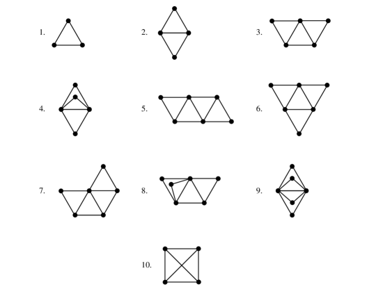
Figure 1: Ten types of cluster

All these types are present in ${\cal S}$ when $\kappa$ is at most 2/3. All other cluster types have expected number tending to $0$ as $\kappa>7/11$, and are therefore are not in ${\cal S}$. Recall that the poset ordering $\prec$ on ${\cal S}$ is not necessarily a linear ordering; for example, the types $\{5,6,7,8,9,10\}$ are all maximal, and therefore not comparable. The ordering $\prec$ is extended to the usual real linear ordering on ${\cal S}$ denoted by $<$.

The first step is to calculate $\lambda_{t}$ for $t\in{\cal S}$. In accordance with (2.4) and (2.5), we obtain the $\lambda_{t}$ as in Table 1.

$\lambda_{1}=\frac{1}{6}[n]_{3}p^{3}$	$\lambda_{2}=\frac{1}{4}[n]_{4}p^{5}$	$\lambda_{3}=\frac{1}{2}[n]_{5}p^{7}$	$\lambda_{4}=\frac{1}{12}[n]_{5}p^{7}$	$\lambda_{5}=\frac{1}{2}[n]_{6}p^{9}$
$\lambda_{6}=\frac{1}{6}[n]_{6}p^{9}$	$\lambda_{7}=\frac{1}{2}[n]_{6}p^{9}$	$\lambda_{8}=\frac{1}{2}[n]_{6}p^{9}$	$\lambda_{9}=\frac{1}{48}[n]_{6}p^{9}$	$\lambda_{10}=\frac{1}{24}[n]_{4}p^{6}$

Table 1: Expected numbers of small clusters.

Our next task is to find the polynomial $\xi_{t,\epsilon}$ of Corollary 2.7 for all $t\in{\cal S}$. For this, the proof of the corollary describes an iterative scheme to compute the $F_{t}^{(r)}$ and hence $\overline{\gamma}^{(r)}_{t}$.

We can drop all terms that would yield coefficients of variables $g_{t_{i}}$ that are $O(n^{-\overline{\epsilon}}/\lambda_{t})$ for some $\overline{\epsilon}>0$. This is because in $\xi_{t,\epsilon}(f)$, each $g_{t_{i}}$ is assigned a value that is $n^{o(1)}$, and hence the dropped terms are subsumed into the error term in (2.56) when $\overline{\epsilon}$ is sufficiently small (recalling that $\overline{\gamma}_{t}(f)\sim 1$ by Lemma 2.5). For similar reasons, we can drop any $O(p^{2})$ term in the expansion of $c(t,t,{\bf 0})$ at the front of (2.58), as $p^{2}\lambda_{t}=O(p^{2}\lambda_{1})=O(p^{5}n^{3})=o(n^{-2/11})$. Note that $c(1,1,{\bf 0})=1-p^{3}$ since it is simply the probability that three vertices do not form a triangle. Hence, we can treat $c(1,1,{\bf 0})$ as 1. A similar argument applies to $c(t,t,{\bf 0})$ for all other $t\in{\cal S}$.

Moving on to the quantities $c(u,t,h)$ inside the summation in (2.58), for any non-zero $h\in{\cal F}$, clearly $c(t,t,h)=O(p^{3})$, and so these terms can be ignored completely for the same reason, for all $t$.

For the other terms in the summation, we only need to compute $c(u,t,h)$ to $O(n^{-\overline{\epsilon}}/\lambda_{u})$. For $u=2$, note that $n^{-\overline{\epsilon}}/n^{4}p^{5}=\Omega(p^{10/7})$ for sufficiently small $\overline{\epsilon}$ since $n<p^{-11/7}$. Thus, we may drop $p^{2}$ terms in $c(2,t,h)$. First consider $c(2,1,{\bf 0})$. In (2.1), $J$ is a cluster of type 2, i.e. (the edge set of) two triangles with a common edge. $Q$ corresponds to one of the two triangles of $J$ (so there are two choices for $Q$). There are four cases for $H$, as it must contain $J\setminus Q$ but no triangles. Letting $q=1-p$, we get

$$c(2,1,{\bf 0})=2(q^{3}+2pq^{2}+p^{2}q)=2(1-p)+O(p^{2}).$$

The other cases of $c(2,t,h)$ can be computed similarly, and only $h=\delta_{1}$ is significant (i.e. not $O(p^{2})$). Similarly, for $u=3$, $1/n^{5}p^{7}=\Omega(p^{6/7})$ and we may drop the $O(p)$ terms. The same clearly holds for all $u>3$ as well. In this way, we obtain all significant terms of $c(u,t,h)$ for $u>t$, as shown in Table 2. In computing these, note that $h$ is quite restrictive. For instance, for $c(3,1,{\bf 0})$, the deletion of $Q$ from $J$ must leave no triangles, and there is only one such choice for $Q$.

$u$	t	h	$c(u,t,h)$	cofactor
2	1	${\bf 0}$	$2(1-p)$	$\frac{3}{2}np^{2}\cdot\overline{\gamma}_{2}$
2	1	$\delta_{1}$	$2p$	$\frac{3}{2}np^{2}\cdot\overline{\gamma}_{2}g_{1}\overline{\gamma}_{1}^{-1}$
3	1	${\bf 0}$	$1$	$3n^{2}p^{4}\cdot\overline{\gamma}_{3}$
3	1	$\delta_{1}$	$2$	$3n^{2}p^{4}\cdot\overline{\gamma}_{3}g_{1}\overline{\gamma}_{1}^{-1}$
4	1	${\bf 0}$	$3$	$\frac{1}{2}n^{2}p^{4}\cdot\overline{\gamma}_{4}$
5	1	$\delta_{1}$	$2$	$3n^{3}p^{6}\cdot g_{1}$
5	1	$\delta_{2}$	$2$	$3n^{3}p^{6}\cdot g_{2}$
6	1	${\bf 0}$	$1$	$n^{3}p^{6}$
6	1	$2\delta_{1}$	$3$	$n^{3}p^{6}\cdot g_{1}^{2}$
7	1	$\delta_{1}$	$2$	$3n^{3}p^{6}\cdot g_{1}$
7	1	$\delta_{2}$	$2$	$3n^{3}p^{6}\cdot g_{2}$
8	1	${\bf 0}$	$1$	$3n^{3}p^{6}$
8	1	$\delta_{1}$	$2$	$3n^{3}p^{6}\cdot g_{1}$
8	1	$\delta_{2}$	$1$	$3n^{3}p^{6}\cdot g_{2}$
9	1	${\bf 0}$	$4$	$\frac{1}{8}n^{3}p^{6}$
10	1	${\bf 0}$	$4$	$\frac{1}{4}np^{3}$

3	2	${\bf 0}$	$2$	$2np^{2}\cdot\overline{\gamma}_{3}$
4	2	${\bf 0}$	$3$	$\frac{1}{3}np^{2}\cdot\overline{\gamma}_{4}$
5	2	${\bf 0}$	$1$	$2n^{2}p^{4}$
5	2	$\delta_{1}$	$2$	$2n^{2}p^{4}\cdot g_{1}$
6	2	${\bf 0}$	$3$	$\frac{2}{3}n^{2}p^{4}$
7	2	${\bf 0}$	$1$	$2n^{2}p^{4}$
7	2	$\delta_{1}$	$2$	$2n^{2}p^{4}\cdot g_{1}$
8	2	${\bf 0}$	$3$	$2n^{2}p^{4}$
8	2	$\delta_{1}$	$1$	$2n^{2}p^{4}\cdot g_{1}$
9	2	${\bf 0}$	$6$	$\frac{1}{12}n^{2}p^{2}$
10	2	${\bf 0}$	$6$	$\frac{1}{6}p$
5	3	${\bf 0}$	$2$	$np^{2}$
6	3	${\bf 0}$	$3$	$\frac{1}{3}np^{2}$
7	3	${\bf 0}$	$2$	$np^{2}$
8	3	${\bf 0}$	$2$	$np^{2}$
8	4	${\bf 0}$	$1$	$6np^{2}$
9	4	${\bf 0}$	$4$	$\frac{1}{4}np^{2}$

Table 2: Significant contributions to (2.58)

The “cofactor” column of Table 2 shows the significant contribution to those terms in $F_{t}$ from

$$\frac{\lambda_{u}}{\lambda_{t}}\overline{\gamma}_{u}\prod_{i=1}^{k}\frac{g_{t_{i}}}{\overline{\gamma}_{t_{i}}}.$$

Here, and in the rest of the calculation, we assume $\overline{\epsilon}>0$ is as small as we like, and any terms that are $O(n^{-\overline{\epsilon}}/\lambda_{t})$ are dropped. In each case, $\lambda_{u}/\lambda_{t}$ is the first item in the column, with any others (that are not equal to 1) appearing after “$\cdot$”. In each case only the leading term of $\lambda_{u}/\lambda_{t}$ turns out to be significant, since the correction terms are $O(1/n)$ and $\lambda_{u}/n=O(n^{3}p^{5})$ for $u\geq 2$. Any other factors which appear to be missing have simply been replaced by 1, with the following justification. In the initial iteration, for computing $F_{t}^{(1)}$ we have all $\overline{\gamma}_{v}$ equal to 1, and by induction, thereafter they are $1+O(np^{2})$ (if we treat each $g_{t_{i}}$ as 1). In the end each $g_{t_{i}}$ is substituted by something that is $n^{o(1)}$. Hence we may set any $\overline{\gamma}_{u}$ or $\overline{\gamma}_{t_{i}}$ equal to 1 in all iterations for all $u\geq 5$, since then $\lambda_{u}np^{2}=O(n^{7}p^{11}+n^{5}p^{8})=O(n^{-\overline{\epsilon}}/\lambda_{t})$. Of course there are no contributions from $t\geq 5$ since all such $t$ are maximal in ${\cal S}$, and $c(u,t,h)=0$ unless $t\prec u$ (and we have already dealt with the case $u=t$).

The significant terms of (2.58) are now deduced to be

$$F_{1} = -np^{2}\left(3(1-p)\overline{\gamma}_{2}+3p\overline{\gamma}_{2}g_{1}/\overline{\gamma}_{1}\right)-n^{2}p^{4}\left(3\overline{\gamma}_{3}+6\overline{\gamma}_{3}g_{1}/\overline{\gamma}_{1}+\frac{3}{2}\overline{\gamma}_{4}\right)$$

$$-n^{3}p^{6}\left(18g_{1}+15g_{2}+3g_{1}^{2}+\frac{9}{2}\right)-np^{3},$$

$$F_{2} = -np^{2}\left(4\overline{\gamma}_{3}+\overline{\gamma}_{4}\right)-n^{2}p^{4}\left(10g_{1}+25/2\right)-p,$$

$$F_{3} = -7np^{2},$$

$$F_{4} = -7np^{2},$$

$$F_{t} = 0\quad\mbox{($t\geq 5$)}.$$

Write $y=np^{2}$ and solve (2.58) iteratively as described after that equation. It may help to note that any terms of order $yp^{2}$, $y^{2}p$ or $y^{4}$ can be dropped. After three iterations (actually the expressions don’t change after the second update), the error is of order $x^{4}=\max\{y^{4},p^{4}\}$ by (2.10), which is neglibible for each $t$. This gives $\xi_{t,\epsilon}=1+F_{t}^{(4)}$ given as follows.

$$\xi_{1,\epsilon} = 1-3y+5py-3g_{1}py+\frac{21}{2}y^{2}-6g_{1}y^{2}-\frac{81}{2}y^{3}+36g_{1}y^{3}-3g_{1}^{2}y^{3}-15g_{2}y^{3},$$ (A.1)

$$\xi_{2,\epsilon} = 1-p-5y+\frac{45}{2}y^{2}-10g_{1}y^{2},$$ (A.2)

$$\xi_{3,\epsilon} = 1-7y,$$ (A.3)

$$\xi_{4,\epsilon} = 1-7y.$$ (A.4)

$$\xi_{t,\epsilon} = 1\quad\mbox{ ($t\geq 5$)}.$$ (A.5)

We will evaluate the expressions given in Section 3 with $7/11<\kappa<2/3$, so that ${\cal S}_{1}=[10]$ and ${\cal S}_{0}=\emptyset$ (and actually $y=x$ as per (2.9)). The ultimate result will then be valid for all values of $\kappa>7/11$ by (3.31). We also fix $\epsilon$ in the range $0<\epsilon<7/11-\chi=3/22$. With $\kappa$ and $\epsilon$ in these ranges, the $\xi_{t,\epsilon}$ are given by the expressions (A.1)–(A.5).

The recursive definition (3.5) of $S_{t}$ for $t\leq 10$ starts with $S_{10}=1$ and hence, in (3.9), $P_{10,\kappa}=0$. Hence (just before (3.14)) $A_{10,\kappa}^{(1)}=1$. Of course there are options in choosing $A$’s since they are only determined up to an error term; we use the natural choices.

The next step is to determine $S_{9}$ and $P_{9,\kappa}$. From (3.15), $A_{10,\kappa}^{(2)}=1$. Now (3.16) implies $j^{\ast}=\lambda_{10}$ and hence from (3.17) $A_{10,\kappa}^{(3)}=1$. It is now easy to check that $A_{10,\kappa}^{(4)}=A_{10,\kappa}^{(5)}=1$ at (3.26), and then similarly $A_{10,\kappa}^{(6)}=A_{10,\kappa}^{(7)}=1$. (Much more detail in the steps here is provided in the less trivial case when $t=1$ below.) Finally, we conclude that, at (3.29), $S_{9}(j_{1},j_{2},\ldots,j_{9})\sim e^{\lambda_{10}}$ and then $P_{9,\kappa}=\lambda_{10}$. In the same way one can show that $S_{t}\sim\exp\left(\sum_{u=t+1}^{10}\lambda_{u}\right)$ for $t=8,7,6,5,4$. In particular we have $S_{4}\sim\exp\left(\sum_{u=5}^{10}\lambda_{u}\right)$ and $P_{4,\kappa}=\sum_{u=5}^{10}\lambda_{u}$.

Next consider $S_{3}$ and $P_{3,\kappa}$. We have that $P_{4,\kappa}(\zeta)$ is independent of $\zeta$, and so $A_{4,\kappa}^{(1)}=1$. The ratio in (3.12) is $T_{j}/T_{j-1}=(1-7y)\lambda_{4}(1+O(\eta))/j,$ so $A_{4,\kappa}^{(2)}=1-7y$, $j^{\ast}=(1-7y)\lambda_{4}$ and $A_{4,\kappa}^{(3)}=1-7y$. Moreover, $\log(\lambda_{4}/j^{\ast})=-\log(1-7y)=7y+O(y^{2})=7y+O(\lambda_{4}^{-1})$, so $A_{4,\kappa}^{(4)}=7y$ and

$$\left(\frac{e\lambda_{4}}{j^{\ast}}\right)^{j\ast}=\left(\frac{e}{1-7y}\right)^{\lambda_{4}(1-7y)}=e^{\lambda_{4}+o(1)}$$

from which we deduce $A_{4,\kappa}^{(5)}=1$. Now, $\sum_{i=0}^{\tilde{j}-1}\log\xi_{4,\epsilon}=\tilde{j}\log(1-7y)=-7y(1-7y)\lambda_{4}+o(1)=-7y\lambda_{4}+o(1)$ implies that $A_{4,\kappa}^{(6)}=1-7yg_{4}$ and $A_{4,\kappa}^{(7)}=1-7y$. Because ${P}_{4,\kappa}$ does not depend on $g_{4}$, $\tilde{P}_{4,\kappa}=P_{4,\kappa}=\sum_{u=5}^{10}\lambda_{u}$. Finally, we have

$$S_{3}(j_{1},j_{2},j_{3})\sim\exp\left(\sum_{u=5}^{10}\lambda_{u}+(1-7y)\lambda_{4}\right)$$

and $P_{3,\kappa}=\tilde{P}_{4,\kappa}+\lambda_{4}A_{4,\kappa}^{(7)}=\sum_{u=5}^{10}\lambda_{u}+(1-7y)\lambda_{4}$. Similar analyses which we omit show that

$$S_{2}(j_{1},j_{2})\sim\exp\left((1-7y)(\lambda_{3}+\lambda_{4})+\sum_{u=5}^{10}\lambda_{u}\right).$$

Next, note that $A_{2,\kappa}^{(1)}=1$, $A_{2,\kappa}^{(2)}=A_{2,\kappa}^{(3)}=\xi_{2,\epsilon}$, $j^{*}=\lambda_{2}\xi_{2,\epsilon}$, $A_{2,\kappa}^{(4)}$ is a truncation of the expansion of $1-\log\xi_{2,\epsilon}$, $A_{2,\kappa}^{(5)}=1-\frac{25}{2}y^{2}$, $A_{2,\kappa}^{(6)}$ is the truncation of $1+g_{2}\log\xi_{2,\epsilon}$, which is $1+g_{2}(-p-5y+(10-10g_{1})y^{2})$, and $A_{2,\kappa}^{(7)}=1-p-5y+\frac{45}{2}y^{2}-10g_{1}y^{2}$. Eventually $S_{1}(j_{1})\sim\exp\left(P_{1,\kappa}(\zeta(j_{1}))\right)$ where

$$P_{1,\kappa}=\left(1-p-5y+\frac{45}{2}y^{2}-10g_{1}y^{2}\right)\lambda_{2}+(1-7y)(\lambda_{3}+\lambda_{4})+\sum_{u=5}^{10}\lambda_{u}.$$ (A.6)

The final step of the induction is a little more involved. We have

$$\exp\big{(}P_{1,\kappa}(\zeta(j))-P_{1,\kappa}(\zeta(j-1))\big{)} = \exp\left(\frac{-10y^{2}\lambda_{2}}{\lambda_{1}}\right)$$

$$= \exp\left(-15y^{3}+O(y^{3}/n)\right)$$

and hence $A^{(1)}_{1,\kappa}=1-15y^{3}$. For (3.15) we set $g_{2}=0$ to get $\tilde{\xi}_{1,\epsilon}$ and obtain

$$A_{1,\kappa}^{(2)}=1+c_{1}+c_{2}g_{1}+c_{3}g_{1}^{2}.$$

where

$$c_{1} = -3y+5py+\frac{21}{2}y^{2}-\frac{81}{2}y^{3}-15y^{3}$$

$$= -3y+5py+\frac{21}{2}y^{2}-\frac{111}{2}y^{3},$$

$$c_{2} = -3py-6y^{2}+36y^{3}$$

$$c_{3} = -3y^{3},$$

The equation (3.16) for $j^{*}$ becomes

$${j^{*}\over\lambda_{1}}=1+c_{1}+c_{2}\left(\frac{j^{*}}{\lambda_{1}}\right)+c_{3}\left(\frac{j^{*}}{\lambda_{1}}\right)^{2}.$$ (A.7)

Since the $c_{i}$ are $O(y^{i})$, $j^{*}\sim\lambda_{1}$ and $\lambda_{1}y^{4}=o(1)$, we find iteratively that $j^{*}=(1+c_{1}+c_{2}+c_{1}c_{2}+c_{3})\lambda_{1}+o(1)$, and so

$$A_{1,\kappa}^{(3)}=1+c_{1}+c_{2}+c_{1}c_{2}+c_{3}.$$ (A.8)

Expanding $1-\log A_{1,\kappa}^{(3)}$ gives

$$A_{1,\kappa}^{(4)}=1-c_{1}-c_{2}-c_{3}+c_{1}^{2}/2-c_{1}^{3}/3$$

and then truncating $A_{1,\kappa}^{(3)}\cdot A_{1,\kappa}^{(4)}$ gives

$$A_{1,\kappa}^{(5)}=1-c_{1}c_{2}-c_{1}^{2}/2+c_{1}^{3}/6.$$

Next, referring to (A.9) and writing $\tilde{c}_{1}=c_{1}+15y^{3}$,

$$\sum_{i=0}^{\tilde{j}-1}\log\xi_{1,\epsilon}(f_{1,i}) = \sum_{i=0}^{\tilde{j}-1}\log\left(1+\tilde{c}_{1}+{c_{2}i\over\lambda_{1}}+{c_{3}i^{2}\over\lambda_{1}^{2}}\right)$$

$$= o(1)+\sum_{i=0}^{\tilde{j}-1}\bigg{(}\tilde{c}_{1}-\frac{\tilde{c}_{1}^{2}}{2}+\frac{\tilde{c}_{1}^{3}}{3}+\frac{(c_{2}-\tilde{c}_{1}c_{2})i}{\lambda_{1}}+\frac{c_{3}i^{2}}{\lambda_{1}^{2}}\bigg{)}$$

$$= \left[\left(\tilde{c}_{1}-{1\over 2}\tilde{c}_{1}^{2}+{1\over 3}\tilde{c}_{1}^{3}\right){\tilde{j}\over\lambda_{1}}+\left({1\over 2}c_{2}-{1\over 2}\tilde{c}_{1}c_{2}\right)\left({\tilde{j}\over\lambda_{1}}\right)^{2}+{1\over 3}c_{3}\left({\tilde{j}\over\lambda_{1}}\right)^{3}\right]\lambda_{1}+o(1),$$

so

$$A_{1,\kappa}^{(6)}=1+\left(c_{1}-{1\over 2}c_{1}^{2}+{1\over 3}c_{1}^{3}\right)g_{1}+\left({1\over 2}c_{2}-{1\over 2}c_{1}c_{2}\right)g_{1}^{2}+{1\over 3}c_{3}g_{1}^{3}.$$ (A.9)

Substituting (A.8) for $g_{1}$ in (A.9), dropping insignificant terms, and adding $-1+A_{t,\kappa}^{(5)}$, we obtain after some algebra

$$A_{1,\kappa}^{(7)} = 1+\tilde{c}_{1}+\tilde{c}_{1}c_{1}-\frac{1}{2}\tilde{c}_{1}^{2}+\frac{1}{2}c_{2}+\frac{1}{2}\tilde{c}_{1}c_{2}+\frac{1}{3}\tilde{c}_{1}^{3}-\frac{1}{2}\tilde{c}_{1}^{2}c_{1}+\frac{1}{3}c_{3}-\frac{1}{2}c_{1}^{2}+\frac{1}{6}c_{1}^{3}+o(\lambda_{1}^{-1})$$

$$= 1-3y+\frac{7}{2}py+\frac{15}{2}y^{2}-\frac{29}{2}y^{3}.$$

Since $j^{*}=\lambda_{1}(1+O(y))$, changing from $g_{1}=\tilde{j}/\lambda_{1}$ or $g_{1}={j}^{*}/\lambda_{1}$ to $g_{1}=1$ in (A.6) induces a change to $P_{1,\kappa}$ of order $O((j^{\ast}-\lambda_{1})y^{2}\lambda_{2}/\lambda_{1})=O(y^{3}\lambda_{2})=o(1)$ and therefore $\tilde{P}_{1,\kappa}=P_{1,\kappa}|_{g_{1}=1}$. Finally,

$$P_{0,\kappa} = \tilde{P}_{1,\kappa}(1)+\lambda_{1}A_{1,\kappa}^{(7)}$$

$$= \sum_{u=5}^{10}\lambda_{u}+(1-7y)\lambda_{4}+(1-7y)\lambda_{3}+\left[1-p-5y+\frac{25}{2}y^{2}\right]\lambda_{2}$$

$$+\,\left[1-3y+\frac{7}{2}py+\frac{15}{2}y^{2}-\frac{29}{2}y^{3}\right]\lambda_{1}+o(1).$$

The remaining task is to plug in the expansions for the $\lambda_{t}$’s given in Table 1, simplify, and apply (3.30). Since $p=o(n^{-7/11})$ we approximate $\lambda_{1}$ by $\frac{1}{6}n^{3}p^{3}-\frac{1}{2}n^{2}p^{3}$, whilst for $\lambda_{t}$, $t\geq 2$ only the first order term is important: $\lambda_{2}\sim\frac{1}{4}n^{4}p^{5}$ etc. This determines $P_{0,\kappa}$ and hence the coefficients in the statement of Theorem 1.1, resulting in the statement of Theorem 1.2 for $p<n^{-7/11-\epsilon}$. To relax this to $p=o(n^{-7/11})$, we only need to note that, from this conclusion, all other terms in the series $F$ in Theorem 1.1 must have $i_{\ell}/j_{\ell}\leq 7/11$. Such terms tend to 0 for $p=o(n^{-7/11})$, and the theorem follows.   

Proof of Theorem 1.3

Here we extend the previous proof to obtain the probablity that ${\cal G}(n,m)$ contains no copies of $K_{3}$. The starting point of our analysis is that for $p=d/\xi$ as given by (4.4), from (4.1) and (4.7) we have

$${\bf P}(X=0\mid Y=m)\sim\frac{{\bf P}(X=0)}{\sqrt{2\pi m}\,{\bf P}(Y=m)}.$$ (A.10)

We need to find the asymptotics of ${\bf P}(X=0)$ and ${\bf P}(Y=m)$ in the way described in the last paragraph of Section 4. This requires first finding the asymptotic expansion of $p=d/\xi$, where $\xi=\xi_{0,\epsilon}(n,p,\tilde{\bf g})$.

Table 3 is essentially an extension of Table 2, showing significant contributions to  $F_{t}$ from (2.58) as needed to calculate $\overline{\gamma}_{0}(n,p,\tilde{{\bf g}})$, under the same assumption that $p=O(n^{-7/11-\epsilon})$. Note that $F_{1}$ and $F_{2}$ need to be recomputed in this new clustering as the expression for $\overline{\gamma}_{0}$ contains $\overline{\gamma}_{1}$ and $\overline{\gamma}_{2}$.

Since $\tilde{g}_{0}=m/\lambda_{0}=mp^{-1}{n\choose 2}^{-1}=d/p=\xi=\xi_{0,\epsilon}(n,p,\tilde{\bf g})=\overline{\gamma}_{0}(m\delta_{0})+o(\lambda_{0}^{-1})$ by (4.2), it is straightforward to see that the factors $\tilde{g}_{1}/\overline{\gamma}_{0}$ can at this point be replaced by $1$. Strictly this needs to be justified in the context of the recursive computation of $\xi$ in Corollary 2.7, and this can be seen in a straightforward way by going back to the original equations in Proposition 2.1 with the altered equations and observe that the same argument as in Section 2 applies to these altered equations, resulting in the modified definition of $F_{t}$ in (2.58); alternatively, one could include the factors explicitly and watch them turn naturally into 1. Note that terms like $c(1,0,\delta_{1})$ cannot affect this computation since they contain a factor $g_{t}$ for $t>0$, and to evaluate $\xi$ we must set such $g_{t}$ equal to 0.

The denominator of (2.58) is $c(0,0,{\bf 0})=1-p$ in the case of $t=0$. As with the ${\cal G}(n,p)$ calculation, we can ignore certain terms in the product of $c(u,t,h)$ with its cofactor. In the case of $t=0$, since the final expression we are computing is $\exp(-\lambda_{1}+o(\lambda_{1}))$ and $\lambda_{1}\sim n^{3}p^{3}/6$, we can ignore any terms that are $O(n^{-\overline{\epsilon}}/\lambda_{1})$, i.e. $O(n^{-\overline{\epsilon}}/n^{3}p^{3})$. Note that $\lambda_{0}=n(n-1)p/2$. Since $\overline{\gamma}_{1}$ only arises in terms with a cofactor that is $O(np^{2})$, we ignore terms in its expression that are $O(n^{-\overline{\epsilon}}/n^{4}p^{5})$ such as $p^{2}$. For similar reasons, terms in $\overline{\gamma}_{2}$ of order $O(n^{-\overline{\epsilon}}/n^{5}p^{7})$ are ignored.

$u$	t	h	$c(u,t,h)$	cofactor
0	0	$\delta_{0}$	$p$	$p\cdot\overline{\gamma}_{0}$
1	0	$2\delta_{0}$	$3(1-p)$	$\frac{1}{3}np^{2}\cdot\overline{\gamma}_{1}$
2	0	$4\delta_{0}$	$1$	$\frac{1}{2}n^{2}p^{4}\cdot\overline{\gamma}_{2}$
4	0	$6\delta_{0}$	$1$	$\frac{1}{6}n^{3}p^{6}$
2	1	$2\delta_{0}$	$2$	$\frac{3}{2}np^{2}\cdot\overline{\gamma}_{2}$
3	1	$4\delta_{0}$	$1$	$3n^{2}p^{4}$
4	1	$4\delta_{0}$	$3$	$\frac{1}{2}n^{2}p^{4}$
3	2	$2\delta_{0}$	$2$	$2np^{2}$
4	2	$4\delta_{0}$	$3$	$\frac{1}{3}np^{2}$

Table 3: Significant contributions to (2.58)

Plugging the values in Table 3 into (2.43) or (2.58) gives the following truncated expressions for $\overline{\gamma}_{0}$, $\overline{\gamma}_{1}$ and $\overline{\gamma}_{2}$

$$\overline{\gamma}_{0}=\frac{1}{1-p}\left(1-p\overline{\gamma}_{0}-(1-p)np^{2}\overline{\gamma}_{1}-\frac{1}{2}n^{2}p^{4}\overline{\gamma}_{2}-\frac{1}{6}n^{3}p^{6}\right),$$

$$\overline{\gamma}_{1}=1-3np^{2}\overline{\gamma}_{2}-\frac{9}{2}n^{2}p^{4},$$

and

$$\overline{\gamma}_{2}=1-5np^{2}.$$

Solving for $\overline{\gamma}_{0}$ gives

$$\overline{\gamma}_{0}=1-np^{2}-\frac{49}{6}n^{3}p^{6}+\frac{5}{2}n^{2}p^{4}+np^{3}+\frac{21}{2}n^{3}p^{7}-3n^{2}p^{5}.$$

Using this expression for $\xi$ we find $1/\xi\approx 1+x-\frac{3}{2}x^{2}+\frac{25}{6}x^{3}-xp$ where $x=np^{2}$ and the terms of order $x^{4}$, $x^{2}p$ and $p^{2}$ are omitted. Substituting $p=d/\xi$ into itself three times gives

$$p=d+nd^{3}-nd^{4}+\frac{1}{2}n^{2}d^{5}+\frac{1}{6}n^{3}d^{7}+o(1/n^{3}p^{3}).$$ (A.11)

For $N={{n}\choose{2}}$ and noting $p=d(1+\epsilon)=m(1+\epsilon)/N$ where $\epsilon=O(d^{2}n)$, we have

$${\bf P}(Y=m) = {\bf P}(Y=dN)={N\choose m}p^{dN}{(1-p)}^{N(1-d)}$$

$$\sim \frac{1}{\sqrt{2\pi dN}}\left((1+\epsilon)^{d}\left(\frac{1-d(1+\epsilon)}{1-d}\right)^{1-d}\right)^{N}$$

$$\sim \frac{1}{\sqrt{2\pi m}}\exp\left(-\frac{1}{4}n^{4}d^{5}-\frac{1}{12}n^{5}d^{7}-\frac{1}{48}n^{6}d^{9}+\frac{1}{4}n^{4}d^{6}\right)$$ (A.13)

using (A.11) to determine $\epsilon$. Theorem 1.2 gives ${\bf P}(X=0)$, from which we can again eliminate $p$ using (A.11). Plugging these into (A.10) gives the probability that $X=0$ in $G\in{\cal G}(m,n)$:

$${\bf P}(X=0|Y=m)\sim\exp\left(-\frac{1}{6}n^{3}d^{3}-\frac{1}{8}n^{4}d^{6}\right).$$

For the same reasons as in the ${\cal G}(n,p)$ case, the validity extends to all $d=o(n^{-7/11})$.

References

[1] B. Bollobás, Random graphs, In Combinatorics, Proceedings (Swansea, 1981), pp. 80–102, London Math. Soc. Lecture Note Ser. 52, Cambridge Univ. Press, Cambridge, 1981.
[2] P. Erdős, D.J. Kleitman and B.L. Rothschild, Asymptotic enumeration of -free graphs, Colloquio Internazionale sulle Teorie Combinatorie (Rome, 1973), Tomo II, pp. 19 27. Atti dei Convegni Lincei, No. 17, Accad. Naz. Lincei, Rome, 1976.
[3] A. Frieze, On small subgraphs of random graphs. In
Random Graphs, Volume 2, Wiley, New Tork, (1992), 67–90.
[4] S. Janson, T. Łuczak and A. Ruciński,
An exponential bound for the probability of nonexistence of a specified subgraph in a random graph, in: M. Karoński, J. Jaworski, A. Ruciński, eds., Random Graphs ’87 (Wiley), pp. 73–87, 1990.
[5] S. Janson, T. Łuczak and A. Ruciński,
Random graphs. Wiley, New York, 2000.
[6] T. Łuczak, On triangle-free random graphs, Random Structures & Algorithms16 (2000), 260–276.
[7] D. Osthus, H.J. Prömel and A. Taraz, For which densities are random triangle-free graphs almost surely bipartite? Paul Erdős and his mathematics (Budapest, 1999). Combinatorica23, 105–150.
[8] H.J. Prömel and A. Steger [8]
Counting -free graphs.
Discrete Math., 154 (1996), 311–315.
[9] H.J. Prömel and A. Steger,
On the asymptotic structure of sparse triangle free graphs,
J. Graph Theory, 21 (1996), 137–151.
[10] A. Ruciński, When are small subgraphs of a random graph normally distributed? Probab. Theory Related Fields78 (1988), 1–10.
[11] N.C. Wormald, The perturbation method and triangle-free random
graphs, Random Structures & Algorithms, 9 (1996), 253–270.