Knot Invariants and M-Theory I: Hitchin Equations, Chern-Simons Actions, and the Surface Operators

Abstract:

Recently Witten introduced a type IIB brane construction with certain boundary conditions to study knot invariants and Khovanov homology. The essential ingredients used in his work are the topologically twisted ${\cal N}=4$ Yang-Mills theory, localization equations and surface operators. In this paper we extend his construction in two possible ways. On one hand we show that a slight modification of Witten’s brane construction could lead, using certain well defined duality transformations, to the model used by Ooguri-Vafa to study knot invariants using gravity duals. On the other hand, we argue that both these constructions, of Witten and of Ooguri-Vafa, lead to two different seven-dimensional manifolds in M-theory from where the topological theories may appear from certain twisting of the G-flux action. The non-abelian nature of the topological action may also be studied if we take the wrapped M2-brane states in the theory. We discuss explicit constructions of the seven-dimensional manifolds in M-theory, and show that both the localization equations and surface operators appear naturally from the Hamiltonian formalism of the theories. Knots and link invariants are then constructed using M2-brane states in both the models.

1 Introduction and summary

Knot theory has attracted both mathematicians and physicists to tackle some of the challenging problems. There are various approaches of constructing invariants of knots and links. Mathematicians put forth skein/recursion relation [1] to evaluate the invariants. The skein method involves study of knots projected onto two dimensions. These invariants can also be obtained from braid group representations deduced from the two dimensional statistical mechanical models, rational conformal field theories and quantum groups. All these approaches show that the invariants are Laurent polynomials in variable $q$ with integer coefficients. That is, for any knot ${\bf K}$:

$$J({\bf K},q)=\sum_{n}a_{n}q^{n},$$ (1)

where $a_{n}$ are integers.

On the other hand, Chern-Simons gauge theory based on any compact group $G$ provides a natural framework to study knots and their invariants [2]. In particular, this approach gives a three-dimensional definition for knots and links. For any knot ${\bf K}$ carrying representation $R$ of gauge group $G$, the expectation value of Wilson loop operator $W({\bf K},R)={\rm Tr}_{R}P~{}\exp\left(\oint_{\bf K}A\right)$ gives the knot invariants:

$$J({\bf K},R,q) = \langle W({\bf K},R)\rangle$$

$$= \int{\cal D}A~{}{\rm exp}\left[ik\int_{{\bf R}^{3}}{\rm Tr}\left(A\wedge dA+{2\over 3}A\wedge A\wedge A\right)\right]{\rm Tr}_{R}P~{}{\rm exp}\left(\oint_{\bf K}A\right),$$

with the first trace being in the adjoint representation, and the second trace ${\rm Tr}_{R}$ being in the representation $R$ of $G$; and $k$, an integer giving the coupling constant that we can use to write $q$ in the following way:

$$q={\rm exp}\left({2\pi i\over k+h}\right),$$ (3)

where $h$ is the dual coxeter number for group $G$. The Jones and HOMFLY-PT polynomials correspond to placing defining representations of $SU(2)$ and $SU(N)$ respectively. Additionally, the skein relation obtained from $SU(N)$ Chern-Simons theory resembles skein relation of Alexander polynomial when $N=0$. Similarly for the defining representation of $SO(N)$, we get Kauffman polynomials. Besides the well known polynomials, we can obtain many new generalised knot invariants [3]. Within this theory having manifest three-dimensional symmetry, it is not obvious as to why these knot invariants have to be Laurent polynomials with integer coefficients. Giving a topological interpretation to these integer coefficients is one of the challenging problem which has been addressed by both mathematicians and physicists during the last 17 years.

An understanding of this issue came from the works on homological invariants initiated by Khovanov [4]. In this interesting work, Khovanov argued that the integer coefficients can be accounted as dimensions of vector spaces. This imples, for any knot ${\bf K}$, Khovanov polynomial will be:

$${\rm Kh}({\bf K},q,t)=\sum_{i,j}t^{i}q^{j}{\rm dim}~{}H_{i,j},$$ (4)

where ${\rm dim}~{}H_{i,j}$ is the dimension of the bigraded homological chain complex. Taking $t=-1$, the above invariant is the $q$-graded Euler characteristic of the homology which gives Jones polynomial (for $G=SU(2)$), namely:

$$J({\bf K},\square,q)=\sum_{i,j}(-1)^{i}q^{j}{\rm dim}~{}H_{i,j}.$$ (5)

Generalisations of the bigraded homological theory for $sl_{3}$ [5], $sl_{N}$ [6] and arbitrary colors which are referred to as categorifications of knot polynomials leading to vector spaces have been extensively studied.

Parallel development from topological string duality conjecture proposed by Gopakumar-Vafa [7] followed by Ooguri-Vafa [8] conjecture for knots have shown that these invariants and their reformulations can be interpreted as counting of BPS states in string theory. Interestingly, this approach led to various checks of integrality properties of generalised knot invariants [9]. Further the works on categorifications motivated the study of triply graded polynomials discussed in [10] succinctly within the string theory context.

More recently, with the aim of interpreting Khovanov homology within intersecting brane model, Witten considered the NS5-D3 brane system to study four dimensional gauge theory on ${\bf W}\times{\bf R}^{+}$ with knots ${\bf K}$ stuck on the three dimensional boundary ${\bf W}$ [11]. Interestingly, the number of solutions $a_{n}$ to the Hitchin equation in the four-dimensional gauge theory, for a given instanton number $n$, now give topological meaning to the integer coefficients in the Laurent polynomials (1). The homological invariants involve one more variable $t$ besides the already existing variable $q$, and require study of the surface operators in a five dimensional theory.

A relation between Witten’s brane setup [11] and the Ooguri-Vafa [8] approach with intersecting D4-branes has been studied in section 5 of [11]. However a more generic construction that relates the four-dimensional ${\cal N}=4$ model of Witten to the ${\cal N}=1$ set-up of Ooguri-Vafa has not been spelled out in full generalities. In this detailed paper, we will study a unified setting in low energy supergravity description of M-theory where we relate the brane setup of Witten with the Ooguri-Vafa string theory background. Specifically we focus on reproducing all the results of Witten in the supergravity picture. Further, we also detail the construction of oper equation useful for the study of knots stuck at the three-dimensional boundary.

1.1 Organization and summary of the paper

This paper is organized in two broad topics. On one hand, we analyze in details the model studied by Witten in [11]. On the other hand we discuss, albeit briefly, the model studied by Ooguri-Vafa [8], pointing out some of the key ingredients that may link various aspects of the two models [11] and [8].

We start section 2 by introducing the two models in question. In section 2.1 we discuss the brane constructions associated with the two models, and argue how they can stem from similar brane configurations. This is of course a first hint to show that the two pictures in [11] and [8] may not be so different as they appear on first sight. However subtlety lies in the construction of the Ooguri-Vafa [8] model because there are at least two possible realizations of the model $-$ one in type IIB and the other in type IIA. Additionally, because of the large $N$ nature of [8], there are also gravity duals in each pictures that may be used to study the model. This is illustrated in section 2.2, where certain issues related to knot configurations are being pointed out.

Section 3 is dedicated completely to analyzing the physics of Witten’s model [11] using a dual configuration in M-theory that has only geometry and fluxes and no other branes except the M2-branes. The technique considered in our work is very different from what is utilized in [11]. Witten uses mostly brane configurations and tactics of four-dimensional ${\cal N}=4$ gauge theory, along with its topological twist, to discuss the physics of knots in the three-dimensional boundary ${\bf W}$. In fact in the notation of [11], the four-dimensional space will be denoted by ${\bf V}$ such that ${\bf V}={\bf W}\times{\bf R}^{+}$, where ${\bf R}^{+}$ is a half-line. Our approach will be to use eleven-dimensional M-theory to study similar physics on the boundary ${\bf W}$. Question naturally arises as to how could two wildly different methods lead to the same physics on ${\bf V}$ as well on the boundary ${\bf W}$. Elaborating this is of course one of the purposes of section 3, but before we summarize the story, let us discuss Witten’s model in some details below.

The work of Witten [11] utilizes certain crucial ingredients useful in studying knots on the boundary ${\bf W}$. The first is the topological theory on ${\bf W}$. In [11] this is achieved in two steps using an intersecting NS5-D3 brane configuration shown in Table 1. The details are discussed in section 3.1.

The second is the localization equations that are not only responsible in simplifying the path integral formalism of the theory, but also helpful in fixing the boundary terms discussed above. We will call these localization equations as BHN equations, the acronym being related to Bogomolnyi, Hitchin and Nahm. A derivation of the BHN equations, using techniques different from what is being used in [11], is presented in section 3.2.10. It turns out, and as explained in [11] and [13], the number of solutions of the BHN equations, for a given instanton number, determines the coefficient of the knot polynomial. In other words, if we express the Jones’ polynomial as (1), then $a_{n}$ is the number of solutions to the BHN equation with instanton number $n$. This accounts for the integer coefficients in the knot polynomials.

The knots appear as Wilson loops in the boundary theory. In the S-dual picture the knots are given by ’tHooft loops. There are some advantages in discussing the S-dual story, particularly in connection with solving the BHN equation, and this forms the third crucial feature of Witten’s work [11]. In section 3.2.13 we use our technique to analyze the S-dual picture, putting special emphasis on the form of the BHN equations.

There is yet another way to study the knots in the theory involving co-dimension two operators, both in the boundary ${\bf W}$ as well as in the bulk ${\bf V}$. These are called the surface operators, and is the fourth crucial ingredient in Witten’s work [11]. We discuss the surface operators in section 3.3.1, and as before show that most of the results studied in [11] do also appear from our analysis.

Finally, Witten discusses a possible realization of the Ooguri-Vafa model [8] given in terms of intersecting D4-branes. Similar analysis is also studied by Walcher [43]. Our study in section 4 differs from both Witten and Walcher analysis as we discuss the D6-branes’ realization of the Ooguri-Vafa model using the brane set-up in Table 2. Although this is intimately connected to the minimally supersymmetric four-dimensional gauge theory, the specific realization of knots in this picture is more subtle. This is elaborated in sections 4.1.1 and 4.4.

From the above discussions we see that the general picture developed by Witten and Ooguri-Vafa in [11] and [8] respectively, may be addressed in a different, albeit unified, way by dualizing the brane configurations of Table 1 and Table 2 to M-theory. The duality proceeds via an intemediate configuration in type IIB involving wrapped five-branes on two-cycles of certain non-Kähler manifolds. The choice of the non-Kähler manifolds remain specific to the model that we want to analyze. For example, Witten’s model dualizes to a configuration of D5-${\overline{\rm D5}}$ branes wrapped on a warped Taub-NUT space as shown in section 3.2. This Taub-NUT space, or more appropriately a warped ALE space, is very different from the ALE space that may appear from T-dualizing the NS5-brane in Table 1. The latter creates problem in path integral representation because of the lack of a global one-cycle rendering it useless to study Khovanov homology. The Taub-NUT that we study here is different as discussed in section 3.2 and we do not use it to study Khovanov homology. Instead our configuration is only used to study knots in the three-dimensional boundary ${\bf W}$.

However, restricting the knots to the three-dimensional boundary is non-trivial. In Witten [11] this is achieved by switching on the gauge theory $\theta$ angle. In our supergravity approach in type IIB, as we show in sections 3.2.1 and 3.2.2, this may be achieved by switching on a non-commutative or a RR deformation on the wrapped five-branes. Interestingly, as we argue in section 3.2.2, these two deformations have similar four-dimensional physics when it comes to restricting the knots to the boundary ${\bf W}$.

The M-theory uplift of the type IIB configuration is then elaborated in section 3.2.3. This is the dual description of Witten’s model in the absence of the knots (knots will be inserted later), and consists of only geometry and fluxes with no branes other than the M2-branes. In this section we argue how the precise geometric information is essential to derive the harmonic two-form which is normalizable and unique. This two-form is essential to derive the $U(1)$ gauge theory on ${\bf V}$. This is elaborated in section 3.2.4, first by ignoring certain backreactions, and then in section 3.2.5, by including all possible backreactions.

The $U(1)$ theory is of course only a toy model, and what we need is the full non-abelian theory in four-dimensional space ${\bf V}$. This is achieved in section 3.2.6, where the first appearance of the M2-branes wrapped on the two-cycles of certain warped multi Taub-NUT space occurs. All these lead to the non-abelian theory on ${\bf V}$, whose details are analyzed in the subsequent sections. In section 3.2.7 we introduce the boundary dynamics.

In sections 3.2.8 and 3.2.9 we present our first set of major computations, related to the four-dimensional scalar fields. The complete interacting lagrangian is derived from M-theory dimensionally reduced over a seven-dimensional manifold of the form (161). It turns out that the dynamics of three scalar fields that are dimensional reduction of the seven-dimensional gauge fields are somewhat easier to derive than the other three scalar fields that are fluctuations of the multi Taub-NUT space. The two sections 3.2.8 and 3.2.9 are elaborations on this.

We then combine everything and write the complete four-dimensional action as (3.2.10). The action contains two pieces: a topological piece and a non-topological piece. This is the start of section 3.2.10, being one of the important section of the paper. The action computed in (3.2.10) now leads succinctly to the total Hamiltonian (167). This is the central result of the paper, from where all other results are derived by minimization and other techniques. For example the BPS equations from the Hamiltonian (167) may be studied by minimizing. The first set of BPS equations appear in (3.2.10) for the gauge choice (170). As we showed in details, for example in (3.2.10), the coefficients computed in sections 3.2.5, 3.2.8, and 3.2.9 solve all the BPS equations (3.2.10) precisely!

The second set of BPS equations also follow easily from the Hamiltonian (167). Our analysis proceeds by first ignoring the topological piece of the action (3.2.10). The BPS equations turn out to be the BHN equations studied in [11]. The BHN equations are given by (181) and (185), with (185) being further expressed in terms of component equations as (3.2.10). Incidentally, if we change our gauge choice from (170) to (187), the first and the second set of BPS equations change to (3.2.10) and (191) respectively, perfectly consistent to what one would expect from [11].

Among all the crucial ingredients of Witten’s model [11], one that we did not emphasize earlier is the appearance of the parameter $t$. This parameter has appeared before in describing the geometric Langland programme using supersymmetric gauge theories in [12]. In the work of [11], $t$ appears once we try to express the BHN equations in terms of topologically twisted variables. In section 3.2.11 we show how $t$ appears naturally in our set-up too, although all informations that may be extracted from [11] using $t$ may appear from our supergravity analysis without involving $t$. This is to be expected as supergravity data contains all information and there is no need to add new parameters. Nevertheless, as we elaborate in section 3.2.11, one may use supergravity to define $t$ and then use this to extract informations similar to [11]. One immediate advantage of this procedure is for finding the BHN equations once the topological piece in the action (3.2.10) is switched on. For example the BHN equation (218) appears easily now, and the full background equations, including the constraint equations plus the BHN equations, can be presented succinctly as (3.2.11). As mentioned above, all these could be done directly using supergravity without involving $t$, but the use of $t$ avoids certain technical challenges.

We have now assimilated all the ingredients, namely the constraint equations and the BHN equations, to construct the theory on the boundary ${\bf W}$. The crucial ingredients are the electric and the magnetic charges ${\bf Q_{E}}$ and ${\bf Q_{M}}$ respectively that appear in the Hamiltonian (234) which is the modified version of the Hamiltonian (167) once the topological term in the action (3.2.10) is switched on. In section 3.2.12 we compute the two charges and show that the electric charge vanish due to our gauge choice (170), and the magnetic charge is given by (236). After twisting, the magnetic charge combines with the topological piece, now reduced to the boundary ${\bf W}$, to give us the boundary theory. This is easier said than done, because a naive computation yields an incorrect boundary action of the form (237). There are numerous subtleties that one needs to take care of before we get the correct boundary action. These are all explained carefully in section 3.2.12, and the final topological action on ${\bf W}$ is given by (250). This is a Chern-Simons action but defined with a modified one-form field ${\cal A}_{d}$, given by (249), and not with the original gauge field ${\cal A}$. This is one of our main results, and matches well with the one derived in [11] using a different technique. The story can be similarly reproduced in the S-dual picture, and we elaborate this in section 3.2.13. Various subtleties in the S-dual description discussed in [11] also show up in our description.

So far we have managed to reproduce the complete boundary topological theory on ${\bf W}$. Question is, where are the knots in this picture? Section 3.3.1 is dedicated to answering this question. It turns out, one of the key player is the surface operator that will be used to explore the knots and knot invariants in the boundary theory. In this section we start by discussing how the surface operators modify the BHN equations that we studied in section 3.2.10. The surface operators are M2-branes in the theory, but their orientations are different from the M2-branes used earlier in section 3.2.6 to enhance the gauge symmetry from abelian to non-abelian. In fact the M2-brane surface operators are co-dimension two singularities both in the bulk ${\bf V}$ and in the boundary ${\bf W}$, and their configurations are presented in Table 5 and in Table 6 for type IIA and M-theory respectively.

In the language of Table 5, the supersymmetry preserved by the surface operator is ($4,4$). The (4, 4) supersymmetric representation contains a vector multiplet, containing vectors and four scalars all in the adjoint representations of the gauge group, and a hypermultiplet, containing four scalars. If we concentrate only on the hypermultiplet sector then, in the absence of the surface operator, the BHN equations satisfy (296) which are exactly the Hitchin’s equations that one would expect from [32], [33], [34]. In the presence of the surface operators (296) changes to (3.3.1), again consistent with [32], [33], [34]. Interestingly, comparing (3.3.1) with (296) we see that the RHS of the three equations in (296) are now no longer zeroes but proportional to certain source terms parametrized by the triplets ($\alpha,\beta,\gamma$). These triplets can be expressed in terms of supergravity parameters as given in (319), which in our opinion is a new result.

One might also ask how the full BHN and the constraint equations appear in the presence of the surface operators when we consider both the vector and the hypermultiplet of (4, 4) supersymmetry. The results are presented in (3.3.1), and (3.3.1) for the BHN equations and (3.3.1) for the constraint equations.

Having got all the background equations and constraints, our next question is the form of the boundary theory. We follow similar steps as before, and express the Hamiltonian, in the presence of the surface operators, as (3.3.1). The Hamiltonian again can be expressed as sum of squares plus the magnetic charge ${\bf Q_{M}}$. However now it turns out, and as explained in section 3.3.1, that the non-abelian case is in reality much harder to study in the presence of the surface operators. To simplify, we then go to the abelian case and express the BHN and the constraints equations as (340). The magnetic charge is not too hard to find now $-$ it is presented in (3.3.1); and from here the boundary theory on ${\bf W}$ is given by (345) by taking care of similar subtleties as encountered in section 3.2.12.

Construction of knots on the boundary ${\bf W}$ using surface operators now easily follow using the configuration depicted in fig 2 and as given at the start of section 3.3.2. More precisely, the Wilson loop structure that we will consider is as given in (352). i.e using gauge fields parallel to the $x_{1}$ axis. This way we are able to trace all the computations with the same rigor as of the earlier sections.

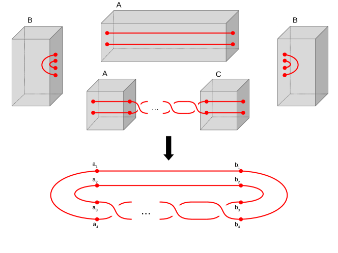
Figure 10: A specific construction of a ($2,n$) torus knot by joining boxes ${\bf A}$, ${\bf B}$ and ${\bf C}$ appropriately. The braid group action now acts $n$ times. The points ($a_{i},b_{i}$) still remain the points where the Wilson lines end on the Heegaard-split manifolds. Once we extend the figure along ${\bf R}_{+}$ (or $\psi$) direction, we will get the configuration of the surface operator.

The next set of computations rely on three crucial steps for the Wilson line configurations. First is the Heegaard splitting (365) as shown in fig 4. Second is the monodromy identifications (374), as shown in fig 6; and third is the braid group action, as shown in fig 5. These three steps form the building blocks for all the knot configurations that we study here. We represent them as operators ${\bf A}_{k}$, ${\bf B}_{k}$ and ${\bf C}_{(2,\sigma_{j})}$ respectively acting on the Wilson line state $|n_{k}\rangle$, where the subscript $k$ denotes the number of Wilson lines; and $\sigma_{j}$ is the braid group action on the $j$-th set of two consecutive Wilson lines. Using the three operators, for example the unknot may be represented as fig 8 and we can use them to compute the knot invariant for this case. However the steps leading to the actual computation of the invariant are riddled with numerous subtleties $-$ dealing with monodromies and framing anomalies to name a few $-$ that we discuss in details in section 3.3.2. The final knot invariant, or more appropriately the linking number for the unknot is given by (376). Similar analysis is presented for the trefoil knot, torus ($2,n$) knots, figure 8 knot and $5_{2}$ knot in (377), (378), (3.3.2) and (3.3.2) respectively. These knot configurations easily follow the three-steps building blocks mentioned above, as shown in fig 9, fig 10, fig 11 and fig 12 respectively, and we discuss how this generalizes to all knot configurations that may be built in our model.

In fact other invariants, beyond the linking numbers, may also be studied for the knot configurations that we discuss here. These invariants have been addressed in [36] and may be constructed using the monodromies ${\cal M}_{k}$ in (367), implying that our analysis is generic enough not only to include all the constructions of [36] but also give them appropriate supergravity interpretations. Despite the success, a non-abelian extension of this picture is harder, and we do not attempt it here leaving a more detailed elaboration for the sequel. Instead however we dedicate the last section, i.e section 3.3.3, albeit briefly on opers that may generalize more easily to the non-abelian case.

Section 4 is dedicated completely in exploring the physics of the Ooguri-Vafa [8] model. From start, there are many points of comparison with section 3 dealing with the physics of Witten’s model [11]. For example, the absence of a Coulomb branch, the location of the knots on the internal ${\bf S}^{3}$ and the existence of a gravity dual might suggest that the Ooguri-Vafa [8] model is very different from Witten’s model [11]. In section 4 we argue that this is not the case. In spirit, these two models are far closer in many respects than one would expect from naive comparison.

The first hint already appears from the discussion in section 5 of [11] and in [43], where the intersecting D4-branes’ construction of the Ooguri-Vafa model is discussed from the brane set-up of Table 1. However we want to emphasize the connection using the brane set-up of Table 2 that directly relates the four-dimensional ${\cal N}=4$ model of Witten to the ${\cal N}=1$ set-up of Ooguri-Vafa.

Our starting point is then multiple D5-branes wrapped on a two-cycle of a non-Kähler resolved conifold. We take $N$ five-branes so that IR gauge group for the minimally supersymmetric four-dimensional gauge theory becomes $SU(N)$. The geometry can be worked out precisely as we show in section 4.1, which in turn is based on the recent work [40]. However existence of a similar picture as in section 3.2.1 without dipole deformation, doesn’t mean that the physics remains similar now. The absence of the Coulomb branch changes the story a bit, and this is discussed in details in section 4.1.1. However the two models, despite the small difference, are identical in some respect regarding the four-dimensional picture, even when we go to the mirror type IIA side. The Ooguri-Vafa model is then realized from the mirror picture by first Euclideanizing the geometry, so that the four-dimensional physics is defined on ${\bf S}^{3}_{(1)}\times{\bf R}^{+}$, and then performing a flop (396) that exchanges the ${\bf S}^{3}_{(1)}$ with ${\bf S}^{3}_{(2)}$, the three-cycle of the mirror deformed conifold. The flop transfers the physics to the three-cycle of the deformed conifold, and this way we can get [8] from [11].

The discussion in section 4.1.1 leaves a few questions unanswered. The first is related to the physics on ${\bf S}^{3}_{(1)}$, namely, what is the precise topological theory on ${\bf S}^{3}_{(1)}$ that we eventually transfer to ${\bf S}^{3}_{(2)}$? The second is related to the knots, namely, what about the knot configurations and the knot invariants? In the remaining part of the paper we answer these two questions.

To answer the first question we will require the precise supergravity background in type IIB, before mirror transformation. This is studied in section 4.2, where the fluxes are worked out in section 4.2.1 and the warp-factors, in the type IIB metric, are worked out in section 4.2.2. The M-theory lift of this configuration is studied in section 4.3.1, where we show that the seven-dimensional manifold is again a warped Taub-NUT fibered over a three-dimensonal base. This time however the warping of the base and fibre in the seven-dimensional manifold (431) is different from what we had in section 3.2.3 such that the four-dimensional supersymmetry can be minimal. Of course the right comparison with section 3.2.3 can only be done after we make a dipole deformation to the type IIB background. It turns out, and as expected, dipole deformation doesn’t break any supersymmetry, but does break the four-dimensional Lorentz symmetry to three-dimensional Lorentz symmetry. This is good because we can localize the knots in the three-dimensional space where there is a manifest Lorentz invariance. Details on this are presented in section 4.3.2.

Once we have the full geometry and fluxes in M-theory, with dipole deformation, it is easy to follow similar procedure as in sections 3.2.3, 3.2.4, 3.2.5 and 3.2.6 to work out the normalizable harmonic forms, and non-abelian enhancement to study the gauge theory in four-dimensional space. This is the content of section 4.3.3, where we discuss the vector multiplet structure, leaving the study of chiral multiplets for the sequel. The vector multiplet structure leads to a non-abelian gauge theory in four-dimensions whose coupling constant, much like (85) before, may to traced to the underlying supergravity variables in M-theory.

The above discussions then brings us to the second question related to the knot configurations and knot invariants. In fact the story is already summarized in section 4.1.1, and in section 4.4 we elaborate on individual steps. The first step is related to the topologically twisted theory on the three-dimensional boundary ${\bf W}$. This time, because of the absence of the Coulomb branch, the boundary theory is simpler than the one in Witten’s model, namely (250). It is now given by (448), which is again a Chern-Simons theory but the coupling constant is not the one that we naively get from the topological piece (447) in M-theory, rather it is a combination that appears from both the G-flux kinetic and the topological pieces in M-theory. This is identical to what we had in section 3.2.12 related to Witten’s model. We now see that a similar structure, yet a bit simpler from [11], is played out for the Ooguri-Vafa model [8] too.

All these are defined on ${\bf S}^{3}_{(1)}$, and once we take the mirror, the theory on ${\bf S}^{3}_{(1)}$ remains identical. The second step is to perform a flop operation (396), so that we can transfer the physics to the three-cycle ${\bf S}^{3}_{(2)}$ of the non-Kähler deformed conifold, giving us (450). For this case, the knots may now be introduced by inserting co-dimension two singularities as depicted in fig 14. Again, the picture may look similar to what we discussed in sections 3.3.1 and 3.3.2, but there are a few key differences. One, we cannot study the abelian version now as the model is only defined for large $N$. This means all the analysis of the knots using operators ${\bf A}_{k}$, ${\bf B}_{k}$ and ${\bf C}_{(2,\sigma_{j})}$ may not be possible now. Two, similar manipulations to the BHN equations that we did in section 3.3.1 now cannot be performed.

What can be defined here? In the remaining part of section 4.4 we give a brief discussion of how to study knots in the Ooguri-Vafa model, leaving a more detailed exposition for the sequel. We summarize our findings and discuss future directions in section 5. In a companion paper [15], and for the aid of the readers, we provide detailed proofs and derivations of all the results here including, at times, alternative derivations of some of the results.

1.2 What are the new results in this paper?

In this paper we construct two different configurations in M-theory, which consist of only geometry, fluxes and M2-branes (the latter provide a non-abelian enhancement of the underlying gauge group). We refer to them as Model A and Model B. These are dual to the models in [11] and [8], respectively. An important new result is that we show the exact duality transformations that relate Models A and B. Consequently, we make explicit the direct connection between the seemingly very distinct models in [11] and [8]. In other words, we provide a unifying picture of the two existing physics approaches to compute knot invariants from the counting of solutions to BPS equations.

The present work focuses on the study of Model A, that dual to the model in [11]. We first obtain the complete four-dimensional gauge theory Lagrangian (3.2.10), appropriatedly compactifying Model A. Then, we derive its associated Hamiltonian (167). Clearly, the coefficients appearing in (167) are expressed in terms of supergravity parameters, by construction. All our results for Model A stem from this Hamiltonian and are mapped in exquisite detail to the results in [11]. We thus conclude that another major outcome of our analysis is that it allows for a precise physical interpretation of [11] in the conceptually simple and long-known classical Hamiltonian formalism. For example, the BPS equations follow from the minimization of (167) for static configurations of the gauge theory fields. We refer to them as BHN equations, the acronym standing for Bogomolnyi-Hitchin-Nahm equations.

The four-dimensional space $\mathbf{V}$ where our Hamiltonian is defined naturally decomposes as $\mathbf{V}=\mathbf{W}\times{\bf R}^{+}$. After minimization of the energy and topologically twisting our theory, we show that the action on the three-dimensional boundary $\mathbf{W}$ of $\mathbf{V}$ is topological. This is a Chern-Simons action for a modified gauge field, which is a certain linear combination of the original gauge fields and some of the scalar fields in our theory. Then, the inclusion of surface operators in this set up provides an inherent framework for realizing knot invariants, as argued in [36]. A key result in our work is the realization of surface operators as M2-branes, different from the ones used for the non-abelian enhancement of Model A. Upon restricting to the abelian case for simplicity, this allows us to work out the linking numbers for the most well-known knots: unknot, trefoil, torus $(2,n)$, figure 8 and $5_{2}$, given by (376)-(3.3.2).

Finally, it is interesting to note that we have not yet exploited most of the immense potential of the constructed Models A and B. To mention a few possibilities, we hope to learn about the Jones, Alexander and HOMFLY polynomials and Khovanov homology in the sequel.

2 Brane constructions and Knots

In this section we will study the knots first from a brane construction proposed by Witten [11, 13] and argue how this could be mapped to the geometric transition picture of Ooguri-Vafa [8, 14]. We will argue that certain fourfolds along with specific configurations of surface operators are useful in making the connections between the two scenarios.

2.1 Brane constructions for Knots

In the original Witten’s construction [11] of knot theory in type IIB theory, we will call this Model A, the branes were arranged as in Table 1,

Directions	0	1	2	3	4	5	6	7	8	9
NS5	$\surd$	$\surd$	$\surd$	$\surd$	$\ast$	$\ast$	$\ast$	$\ast$	$\surd$	$\surd$
D3	$\surd$	$\surd$	$\surd$	$\ast$	$\ast$	$\ast$	$\surd$	$\ast$	$\ast$	$\ast$

Table 1: The orientations of various branes in the intersecting branes set-up. The notation $\surd$ is the direction along which the branes are oriented.

with an additional source for IIB axion, $C_{0}$, switched on such that the knots are localised along the $2+1$ dimensional intersection parametrised by $x_{0,1,2}$.

Let us now modify the original set-up of Witten by converting the direction $x_{6}$ along which the D3-brane is stretched into a finite interval. This is achieved by introducing another NS5-brane oriented along $x_{0,1,2,3,4,5}$. This crucial step will be useful for us to relate the configuration of Witten to the configuration of Ooguri-Vafa [8], as we will soon see. For later convenience we will call this, and the subsequent modification of this, as Model B.

The type IIB configuration can be modified further by T-dualizing along $x_{3}$ direction. This T-duality leads us to the well-known configuration in type IIA theory [16, 17] as depicted in Table 2.

Directions	0	1	2	3	4	5	6	7	8	9
NS5	$\surd$	$\surd$	$\surd$	$\surd$	$\ast$	$\ast$	$\ast$	$\ast$	$\surd$	$\surd$
NS5	$\surd$	$\surd$	$\surd$	$\surd$	$\surd$	$\surd$	$\ast$	$\ast$	$\ast$	$\ast$
D4	$\surd$	$\surd$	$\surd$	$\surd$	$\ast$	$\ast$	$\surd$	$\ast$	$\ast$	$\ast$

Table 2: The orientations of various branes in the T-dual of the modified Witten set-up.

In addition to the required branes we will have a background type IIA gauge field $A_{3}$, that will have a pull-back on the D4-brane and furthermore introduce a non-trivial complex structure on the ($x_{3},x_{6}$) torus. The latter operation will help distinguish the non-compact world-volume directions $x_{0,1,2}$ with the compact toroidal directions even in the limit of large size of the torus. However although supersymmetry of the background still remains valid, the localization of the knots in the $x_{0,1,2}$ directions is not: we have lost the Coulomb branch, so the discussion of knots should be taken with care here. We will study this soon.

Finally let us make yet another modification to the set-up studied above: introduce large $N$ number of D4-branes. Such a modification will help us to study the gravity dual of this set-up, in other words will connect us directly to the model studied by Ooguri-Vafa [8] or more recently to Aganagic-Vafa [14]! This is because an appropriate T-duality to the above brane configuration will convert the two NS5-branes to a singular conifold and the $N$ D4-branes to $N$ wrapped D5-branes on the vanishing two-cycle of the conifold. We can then blow-up the two cycle to convert the singular conifold to a resolved conifold. The D5-branes will then wrap the resolution two-cycle. To see how this works, let us discuss this in some details.

2.2 T-duality, resolved cone and a geometric transition

We begin by introducing a circle action on the conifold and extend it to the resolved conifold in a compatible manner. Consider an action $S_{c}$ on the conifold $xy-uv=0$, where ($x,y,u,v$) are complex coordinates, in the following way:

$$S_{c}:~{}~{}(e^{i\theta},x)\to x,~{}~{}(e^{i\theta},y)\to y,~{}~{}(e^{i\theta},u)\to e^{i\theta}u,~{}~{}(e^{i\theta},v)\to e^{-i\theta}v.$$ (6)

The orbits of the action $S_{c}$ degenerates along the union of two intersecting complex lines $y=u=v=0$ and $x=u=v=0$ on the conifold. Now, if we take a T-dual along the direction of the orbits of the action, there will be NS branes along these degeneracy loci as argued in [18]. So we have two NS branes which are spaced along $x$ (i.e. $y=u=v=0$) and $y$ directions (i.e. $x=u=v=0$) together with non-compact direction along the Minkowski space which will be denoted by $NS_{x}$ and $NS_{y}$.

One may lift this action so as to define a resolved cone. To do that, let us start with two ${\bf C}^{3}$ with coordinates ($Z,X,Y$) and ($Z^{\prime},X^{\prime},Y^{\prime}$) respectively, where ($Z,Z^{\prime}$) are the coordinates of ${\bf P}^{1}$ in the two ${\bf C}^{3}$’s respectively, and the rest form the coordinates of the fiber. Then the manifold ${\cal O}(-1)\oplus{\cal O}(-1)$ over ${\bf P}^{1}$ can be obtained by gluing the two copies of ${\bf C}^{3}$, parametrized above, by the following identification:

$$ZZ^{\prime}=1~{},~{}\quad X^{-1}X^{\prime}=Z~{},~{}\quad Y^{-1}Y^{\prime}=Z.$$ (7)

The blown-down map from the resolved conifold to the conifold ${\cal C}$ is given by eq (7) of [16], from where one may infer the action $S_{r}$ on the resolved conifold to be an extension of the action $S_{c}$ (6) given by by eq (8) of [16]. The rest of the discussion after eq (8) of [16], till the end of section 2 in [16], details how the T-dual picture becomes the following brane configuration: a D4 brane along the interval with two NS branes in the orthogonal direction at the ends of the interval exactly as illustrated in Table 2. Here the length of the interval is the same as the size of the two-cycle of the resolved conifold. As the two-cycle shrinks to zero, the brane construction of a resolved conifold approaches the brane construction of a conifold.

In the language of branes, the two NS5 branes are along directions $x_{4,5}$ and $x_{8,9}$ and fill simultaneously the spacetime directions $x_{0,1,2,3}$. This means the T-duality was done along direction $x_{6}$, or in the language of a conifold, along $\psi$. The conifold geometry is parametrized by ($\theta_{i},\phi_{i}$) with $i=1,2$ with the $U(1)$ direction $\psi$ and the non compact radial direction $r$. In the following let us clarify some subtleties related to the T-duality. First let us consider the wrapped D5-brane on a conifold geometry. A standard T-duality along an orthogonal direction should convert this to a wrapped D6-brane. The $C_{7}$ source charge of the D6-brane decomposes in the following way:

$$C_{7}(\overrightarrow{\bf x},\psi,\theta_{1},\phi_{1})~{}=~{}C_{5}(\overrightarrow{\bf x},\psi)\wedge\left({e_{\theta_{1}}\wedge e_{\phi_{1}}\over\sqrt{V_{2}}}\right)$$ (8)

where $V_{2}$ is the volume of the two-sphere that is being wrapped by the D6-brane and whose cohomology is represented by the term in the bracket. In the limit where the size of the two-sphere is vanishing (i.e for the T-dual conifold), the term in the bracket in (8) will behave as a delta-function, and consequently $C_{7}$ will decompose as $C_{5}$ i.e as a D4-brane. It will take infinite energy to excite any mode along the directions of the vanishing two-sphere, and therefore for all practical purpose a T-dual of the wrapped D5-brane on a conifold will be a D4-brane stretched along $\psi$ direction. This is of course the main content of [20, 21, 19]. Similarly if the wrapped two-sphere is of finite size, i.e the D5-brane wraps the two-cycle of a resolved conifold, then at energy lower than the inverse size of the two-sphere the T-dual will effectively behave again as a D4-brane [16, 17]. Once the energy is bigger than this bound $-$ the size of the two-cycle is much bigger than the string scale $-$ then the intermediate energy physics will probe the full D6-brane. Our analysis in this paper will be related to this case only, i.e we will explore the classical dynamics of a wrapped D6-brane on a four-cycle parametrized by ($\theta_{1},\phi_{1},\psi$) and $x_{3}$.

The above discussion tells us that, under appropriate T-duality, we should get the IR picture of the geometric transition model studied by Ooguri-Vafa [8]. There are of course few differences that we need to consider before making the equivalences. The first is the existence of a $B_{\rm NS}$ field with one of its components along the D5-branes and another orthogonal to it. This $B_{\rm NS}$ field should give rise to the dipole deformations of the D5-branes’ gauge theory [24, 25, 26]. This deformation should also be responsible for preserving supersymmetry in the model. It is however not clear that the knots in this model should again be restricted to $x_{0,1,2}$ directions, although naively one could argue that the two directions of the D5-branes are wrapped on the ${\bf P}^{1}$ of the resolved conifold, and the dipole deformation with a $B_{\rm NS}$ field $B_{3\psi}$ should restrict the knots further to the $x_{0,1,2}$ directions. The reason is of course the absence of the Coulomb branch which is a crucial ingredient in [11, 13].

There is another reason why this should not be the case. We can ask the following question: what will happen if we make a geometric transition to two-cycle on which we have wrapped D5-branes? From standard argument we know that the D5-branes will disappear and will be replaced by fluxes. In this flux picture, or more appropriately the gravity dual, it will be highly non-trivial to get the information about the knots from the fluxes on a deformed conifold background (as there are no branes on the dual side). One might think that a T-dual of this gravity dual could bring us back to branes in type IIA, but this doesn’t help as the original D4-branes on which we had the knot configurations do not appear even on the brane side. To see this, consider the following circle action $S_{d}$:

$$S_{d}:~{}(e^{i\theta},x)\to x,~{}~{}(e^{i\theta},y)\to y,~{}~{}(e^{i\theta},u)\to e^{i\theta}u,~{}~{}(e^{i\theta},v)\to e^{-i\theta}v,$$ (9)

on the deformed conifold $xy-uv=\mu$, where $\mu$ is the deformation parameter. Then $S_{d}$ is clearly the extension of $S_{r}$ discussed in eq (8) of [16], and the orbits of the action degenerate along a complex curve $u=v=0$ on the deformed conifold. If we take a T-dual of the deformed conifold along the orbits of $S_{d}$, we obtain a NS brane along the curve $u=v=0$ with non-compact direction in the Minkowski space which is given by $xy=\mu$ in the x-y plane. Topologically, the above curve is ${\bf R}^{1}\times{\bf S}^{1}$. Thus in the T-dual picture, the large $N$ duality implies a transition from the brane configuration of $N$ coincident D4-branes between two orthogonal NS5-branes to the brane configuration of a single NS5-brane wrapped on ${\bf R}^{1}\times{\bf S}^{1}$ with appropriate background fluxes. The D4-branes have disappeared in the dual brane configuration too, apparently along with our knot configuration!

The solution to the above conundrum is non-trivial and we will discuss this soon. But first let us discuss how to study Model A using the approach of wrapped branes on certain non-Kähler manifolds. This will lead us to a more unified approach to discuss both the models.

3 Model A: The type IIB dual description and warped Taub-NUT

The situation for Model A is slightly different as it is directly related to [11] and therefore to the Chern-Simons theory along $x_{0,1,2}$ directions for the brane configurations given in Table 1. The claim is that the knot polynomial $J(q;{\bf K}_{i},R_{i})$ for any knot ${\bf K}_{i}$ is given in the Chern-Simons theory via the following path integral:

$$J(q;{\bf K}_{i},R_{i}) = \langle{W}({\bf K}_{i},R_{i})\rangle=\langle{\rm Tr}_{R_{i}}P~{}{\rm exp}\oint_{{\bf K}_{i}}A\rangle$$ (10)

$$= {\int{\cal D}A~{}{\rm exp}\left(iS_{cs}\right)\prod_{i}{\cal W}(K_{i},R_{i})\over\int{\cal D}A~{}{\rm exp}\left(iS_{cs}\right)},$$

that is a generalization of (1), and where $q$ is the variable which is used to express the knot polynomial as a Laurent series, $R_{i}$ is the compact representation of the gauge group $G$ appearing in the Chern-Simons action $S_{cs}$:

$$S_{cs}={k\over 4\pi}\int_{\bf W}{\rm Tr}\left(A\wedge dA+{2\over 3}A\wedge A\wedge A\right).$$ (11)

As discussed in the introduction, $k$ is an integer used to express $q$ as in (3). The denominator appearing in (10) is in general non-trivial function of $k$. For example for $SU(2)$ group with ${\bf W}={\bf S}^{3}$, as shown in [2] and [11], the denominator becomes:

$$\int{\cal D}A~{}{\rm exp}\left(iS_{cs}\right)=\sqrt{2\over k+2}~{}{\rm sin}\left({\pi\over k+2}\right),$$ (12)

but if we take ${\bf W}={\bf R}^{3}$, this can be normalized to 1 and so (1) and (10) become identical. This is the case we will study in this section. The above two expressions (10) and (3) serve as dictonary that maps the knot polynomial $J$ and the knot parameter $q$ in terms of the variables of Chern-Simons theory.

3.1 First look at the gravity and the topological gauge theory

We will discuss the knots appearing from this construction soon, but first let us modify Table 1 slightly by first restricting the direction $x_{6}$ to an interval, and secondly, T-dualizing along $x_{3}$ direction to convert the configuration to D4-branes between two parallel NS5-branes. T-dualizing further along $x_{6}\equiv\psi$ direction will convert the D4-branes to fractional D3-branes at a point on a warped Taub-NUT space. In particular, we will have a geometry like:

$$ds^{2}=e^{-\phi}ds^{2}_{0123}+e^{\phi}ds_{6}^{2}$$

$${\cal F}_{3}=e^{2\phi}\ast_{6}d\left(e^{-2\phi}J\right),$$ (13)

where $\phi$ is the dilaton and the Hodge star and the fundamental form $J$ are wrt to the dilaton deformed metric $e^{2\phi}ds_{6}^{2}$. The metric $ds_{6}$ will be given by:

$$ds^{2}_{6}=F_{1}dr^{2}+F_{2}(d\psi+{\rm cos}~{}\theta_{1}d\phi_{1})^{2}+F_{3}(d\theta_{1}^{2}+{\rm sin}^{2}\theta_{1}d\phi_{1}^{2})+F_{4}(dx_{8}^{2}+dx_{9}^{2}),$$ (14)

with $F_{1}=F_{1}(r),F_{2}=F_{2}(r)$ and $F_{3}=F_{3}(r)$ as functions of $r$ only and $F_{4}=F_{4}(r,x_{8},x_{9})$, as the simplest extension of the case with only radially dependent warp factors. Note also that the fractional D3-branes cannot be interpreted as wrapped D5 - ${\overline{\rm D5}}$ branes along ($\theta_{1},\phi_{1}$) directions. Instead the fractional D3-branes will be interpreted here as D5 - ${\overline{\rm D5}}$ pair wrapping direction $\psi$ and stretched along the radial $r$ direction.

We can also change the topology along the $x_{8,9}$ directions from ${\bf R}^{2}$ to ${\bf T}^{2}$ or ${\bf P}^{1}$ without violating Gauss’ law. Before elaborating on this story, let us clarify few issues that may have appeared due to our duality transformation. First, one would have to revist the supersymmetry of the model, which seems to have changed from ${\cal N}=4$ to ${\cal N}=2$. This still allows a Coulomb branch, but we need more scalars to complete the story. One way to regain the lost supersymmetry is to assume that the $x_{6}$ circle is large, so that essentially, for the half space $x_{6}>0$, we have the same physics explored in [12, 11].

Secondly, Witten discusses the possibility of T-duality along orthogonal $S^{1}$ for the D3-NS5 system and argues that, because of the absence of a topological one-cycle in the T-dual configuration, the path integral in this framework cannot be taken as a trace. Our configuration differs from this conclusion in the following way. The T-dual will lead us to a non-Kähler metric on the Taub-NUT space (we call this as a deformed Taub-NUT) and although the Taub-NUT circle will shrink to zero size, we will not be using the Taub-NUT configuration to compute the path integral. Rather a different Taub-NUT will feature later in our study of the gauge theory on the wrapped D5-branes.

Thirdly, converting the D3-branes to D4-branes wrapped along direction $x_{3}$ would seem to give us only two scalars ($x_{8},x_{9}$). But this is not quite the case as the fluctuation of the gauge field along the $x_{3}$ direction will appear as an extra scalar field when we look at the three dimensional gauge theory along directions ($x_{0},x_{1},x_{2}$). These are therefore exactly the scalar $\overrightarrow{X}$ in [11]. The other three scalar fields, namely ($x_{4},x_{5},x_{7}$), are related to $\overrightarrow{Y}$ in [11].

Below a certain energy scale, related to inverse radius of the $x_{3}$ circle, the theory on the D4-branes can be studied at the intersection space of NS5-D4 system. The boundary action is then given, for the Euclidean three dimensional space, by [11]:

$$S^{(1)}_{b}={1\over g^{2}_{YM}}\int_{x_{6}=0}d^{3}x\left[l_{1}\epsilon^{abc}{\rm Tr}~{}X_{a}[X_{b},X_{c}]+l_{2}\epsilon^{\mu\nu\rho}{\rm Tr}\left(A_{\mu}\partial_{\nu}A_{\rho}+{2\over 3}A_{\mu}A_{\nu}A_{\rho}\right)\right],$$

where ($l_{1},l_{2}$) are constants related to the background gauge field $\langle A_{3}\rangle$ (see also [11]) and the superscript is for later convenience.

3.1.1 On the topologically twisted theory

Constructing a topological field theory using R-symmetry twist to ${\cal N}=4$ theory is well known, and could be easily applied to our configuration. The wrapped D4-branes on $x_{3}$ has a $SO(5)$ symmetry broken to $SO(4)\times U(1)$. The one-form associated with the $U(1)$ symmetry can be combined with the twisted scalar fields, i.e scalar fields associated with ($x_{8},x_{9}$) converted to one-forms $\phi_{\mu}dx^{\mu}$. The fluctuation of the gauge field along $x_{3}$ direction contributes another one-form. Finally the fourth one-form may appear from one component of the fluctuations of the D4-branes along orthogonal direction. Together these one-forms could be expressed (in Euclidean space) as:

$$\phi\equiv\sum_{\mu=0}^{3}\phi_{\mu}dx^{\mu},$$ (16)

which captures the concept of R-symmetry twist (see [12, 11] for more details). Using these we can rewrite (3.1) as the following topological theory [11]:

$$S^{(1)}_{b}={1\over g^{2}_{YM}}\int_{x_{6}=0}d^{3}x\epsilon^{\mu\nu\rho}{\rm Tr}\left[2l_{1}\phi_{\mu}\phi_{\nu}\phi_{\rho}+l_{2}\left(A_{\mu}\partial_{\nu}A_{\rho}+{2\over 3}A_{\mu}A_{\nu}A_{\rho}\right)\right],$$ (17)

where the coefficients $l_{1}$ and $l_{2}$ are defined in terms of $t\equiv\pm{|\tau|\over\tau}$, where $\tau$ is the standard definition for four-dimensional gauge theory, namely $\tau={\theta\over 2\pi}+{4\pi i\over g^{2}_{YM}}$, as:

$$l_{1}\equiv-{t+t^{-1}\over 6},~{}~{}~{}~{}~{}~{}~{}l_{2}\equiv{t+t^{-1}\over t-t^{-1}}.$$ (18)

The derivation of the above relations are given in [11], assuming the $\theta$ angle in the definition of $\tau$ to be related to the YM coupling $g^{2}_{YM}$.

The topological theory that we got above in (17) is however not complete. There are other terms that require a more detailed study to derive. The derivation has been beautifully presented in [11], so we will just quote the results. The idea is to take the five-dimensional action on the D4-branes:

$$S_{\rm D4}={1\over g^{2}_{5}}\int d^{5}x\sqrt{g^{(5)}}{\cal L}^{(5)}_{kin}+T_{4}\int\epsilon^{\mu\nu\rho\sigma\alpha}{\cal A}_{\mu}{\rm Tr}~{}F_{\nu\rho}F_{\sigma\alpha},$$ (19)

where $T_{4}$ is the tension of the D4-brane, and reduce over the compact direction $x_{3}$. The expectation value of ${\cal A}_{\mu}$, alongwith $T_{4}$, will give rise to the $\theta$ angle in the dimensionally reduced four-dimensional ${\cal N}=4$ SYM theory with the YM coupling determined by the length $R_{3}$ of the compact $x_{3}$ direction (assuming flat $g^{(5)}$):

$${1\over g^{2}_{YM}}={R_{3}\over g^{2}_{5}}.$$ (20)

The kinetic piece of the five-dimensional action of the D4-branes can now be represented as:

$${1\over g^{2}_{5}}\int d^{5}x\sqrt{g}{\cal L}^{(5)}_{kin}~{}\to~{}{1\over g^{2}_{YM}}\int d^{4}x\sqrt{g}{\cal L}_{kin}=\{Q,....\}$$ (21)

$$~{}~{}~{}~{}~{}+{1\over g^{2}_{YM}}\int d^{3}x{1\over\sqrt{1+w^{2}}}\left[-w\Omega(A)+\epsilon^{\mu\nu\sigma}{\rm Tr}\left(\phi_{\mu}F_{\nu\sigma}+w\phi_{\mu}D_{\mu}\phi_{\sigma}-{2\over 3}\phi_{\mu}\phi_{\nu}\phi_{\sigma}\right)\right]$$

where the bounday integral has to be defined at both ends of $x_{6}$, namely $x_{6}=0$ and $x_{6}\to\infty$, or to the point along $x_{6}$ where we have moved the other NS5-brane. Of course, as mentioned earlier, to preserve maximal supersymmetry, the other NS5-brane has to be kept far away so that near $x_{6}=0$ we restore ${\cal N}=4$ supersymmetry. We have also related $t$, appearing in (18), and $w$ as:

$$t~{}=~{}w-\sqrt{1+w^{2}}.$$ (22)

The other parameters appearing in (21) are defined in the following way: $Q$ is the standard supersymmetric operator such that in the absence of any boundary, the kinetic piece would only be given by the first line of (21) i.e as an anti-commutator with $Q$. The other parameter $\Omega(A)$ is the standard Chern-Simons term in three-dimension, such that:

$$\int d^{3}x~{}\Omega(A)=\int{\rm Tr}\left(A\wedge dA+{2\over 3}A\wedge A\wedge A\right).$$ (23)

It is now easy to see that once we combine the boundary term of (21) with the bounday action (17), the final action takes the following simple form:

$$S=-{4\pi\over g^{2}_{YM}}\cdot{1\over w\sqrt{1+w^{2}}}\int_{x_{6}=0}d^{3}x\int{\rm Tr}\left(A_{w}\wedge dA_{w}+{2\over 3}A_{w}\wedge A_{w}\wedge A_{w}\right),$$ (24)

as one may verify from [11] too. The above action is essentially $\Omega(A_{w})$, with $A_{w}\equiv A+w\phi$. This tells us that we could insert a generalized one-form, given by $A_{w}$, into the Chern-Simons action and get the corresponding topological field theory! This generalized one-form, as we will argue soon, should appear from our M-theory analysis. Note also that the path integral description should remain similar to (10) as:

$$\int{\cal D}A_{w}{\rm exp}\left[{4\pi\over g^{2}_{YM}}\cdot{1\over w\sqrt{1+w^{2}}}\int d^{3}x~{}\Omega(A_{w})\right]~{}=~{}\int{\cal D}A~{}{\rm exp}\left[{4\pi\over{g}^{2}}\int d^{3}x~{}\Omega(A)\right]$$

where we assume that the path integral is evaluated at the usual boundary $x_{6}=0$. Thus the $S_{cs}$ appearing in (10) should then be identified with (23) except with a scaled coupling ${g}^{2}$ defined as:

$${g}=g_{\rm YM}\sqrt{w\sqrt{1+w^{2}}}.$$ (26)

It is important to recall that, for our case, only the low energy dynamics is given by the Chern-Simons theory at the boundary. By low energy we mean the energy scale smaller than the inverse radius of the $x_{3}$ direction. Using the language of [11] our five-dimensional Euclidean space is given by ${\bf V}\equiv{\bf W}\times{\bf S}^{1}\times{\bf R}_{+}$, where ${\bf S}^{1}$ is parametrized by $x_{3}$ and ${\bf R}_{+}$ is parametrized by $x_{6}$. This ${\bf S}^{1}$ should not be confused with the ${\bf S}^{1}$ of [11] used in studying Khovanov Homology.

There is one subtlety that we always kept under the rug: the physics at the other boundary associated with the existence of the second parallel NS5-brane. We had assumed that the second NS5-brane can be moved far away so that near $x_{6}=0$ we have the full ${\cal N}=4$ supersymmetry. Although this description is roughly correct, this is not the full picture as this $x_{6}$ circle will become the Taub-NUT circle in the dual type IIB framework. Therefore it is then necessary to determine the behavior of the following Chern-Simons form:

$$\Omega(A^{(1)}_{w})-\Omega(A_{w}^{(2)}),$$ (27)

where $A^{(1)}_{w}=A_{w}$ is gauge field we studied earlier for the boundary $x_{6}=0$. As discussed by Witten in [11], if we view $A_{w}^{(2)}$ to be trivial, then the path integral can be represented as (3.1.1). We will elaborate on this later.

3.2 Non-abelian extension and Chern-Simons theory

Having developed the basic strategy to study Chern-Simons theory from our brane construction, let us now analyze the geometry (3.1). The $x_{6}$ circle on the brane side will appear as a $S^{1}$, parametrized by $\psi$, fibered over the radial direction. The topology of this space is a $P^{1}$ and it will be assumed that the D5-branes wrap this two-cycle. The $\overline{\rm D5}$-branes are moved away along the Coulomb-branch.

The fundamental form ${\cal J}$ can be computed from (14) using standard procedure, and is given by:

$${\cal J}=\sqrt{F_{1}F_{2}}~{}(d\psi+{\rm cos}~{}\theta_{1}d\phi_{1})\wedge dr+F_{3}~{}{\rm sin}~{}\theta_{1}d\theta_{1}\wedge d\phi_{1}+F_{4}~{}dx_{8}\wedge dx_{9}.$$ (28)

One can plug $J\equiv e^{2\phi}{\cal J}$ in (3.1) to determine the RR three-form flux using Hodge duality. Assuming non-zero background dilaton, this is given by the following expression:

$${\cal F}_{3}=e_{\psi}\wedge\left(k_{1}~{}e_{\theta_{1}}\wedge e_{\phi_{1}}+k_{2}~{}dx_{8}\wedge dx_{9}\right),$$ (29)

where due to the wedge structure there would be no $F_{48}={\partial F_{4}\over\partial x_{8}}$ or $F_{49}$ factors. This is reflected in the coefficients ($k_{1},k_{2}$) which are given in terms of the warp factors of (3.1) as:

$$k_{1}={e^{2\phi}F_{4r}F_{3}\sqrt{F_{2}}\over F_{4}\sqrt{F_{1}}},~{}~{}~{}~{}~{}~{}~{}~{}~{}k_{2}={e^{2\phi}\left(\sqrt{F_{1}F_{2}}-F_{3r}\right)F_{4}\sqrt{F_{2}}\over F_{3}\sqrt{F_{1}}},$$ (30)

even if we keep $\phi$ as an arbitrary, but well defined, function of the internal coordinates. Note that if the metric on the space (3.1) is Kähler, then our formula would have yielded vanishing RR three-form flux. Thus when the D5-branes wrap the two-cycle of a blown-up Taub-NUT space, the metric has to be non-Kähler to preserve supersymmetry.

3.2.1 Generalized deformation and type IIB background

It is now time to see what effect would the introduction of type IIA complex structure on the ($x_{3},\psi$) torus have on our type IIB background. This will not be a dipole deformation, rather it will be a non-commutative (NC) deformation of the wrapped five-brane theory, the non-commutativity only being along the ($x_{3},\psi$) directions. Essentially the simplest non-commutative deformation amounts to switching on a NS B-field with both components along the brane. The B-field for our case will have component $B_{3\psi}$ as we mentioned before, which of course has the required property in the presence of a D5-brane along ($x_{0,1,2,3},r,\psi$). Since the warp factors are $r$ dependent, this B-field component will be a constant along the ($x_{3},\psi$) directions but will depend on the radial coordinate $r$. This case is unlike anything that has been studied so far, although from an effective three-brane point of view this will be a dipole deformation. Thus this is not the standard NC deformation but we will continue calling it one.

We now expect a field strength of the form $dB$. This field strength will then back-react on our original type IIB background (3.1) and change the metric to the following:

$$ds^{2} = e^{-\phi}\left[-dt^{2}+dx_{1}^{2}+dx_{2}^{2}+{dx_{3}^{2}\over{\rm cos}^{2}\theta+F_{2}~{}{\rm sin}^{2}\theta}\right]$$

$$+ e^{\phi}\left[F_{1}dr^{2}+{F_{2}\left({d\psi\over{\rm cos}~{}\theta}+{\rm cos}~{}\theta_{1}d\phi_{1}\right)^{2}\over 1+F_{2}~{}{\rm tan}^{2}\theta}+F_{3}\left(d\theta_{1}^{2}+{\rm sin}^{2}\theta_{1}d\phi_{1}^{2}\right)+F_{4}(dx_{8}^{2}+dx_{9}^{2})\right],$$

where $\theta$ is related to the NC deformation. It is easy to see how the Lorentz invariance along the compact $x_{3}$ direction is broken by the NC deformation. This is one reason (albeit not the most important one) for the knots to be restricted along the Euclidean three directions.

Coming now to the fluxes, it is interesting to note that the RR three-form flux remain mostly unchanged from the value quoted earlier in (29) with a small change in the $d\psi$ fibration structure:

$${\cal F}_{3}=\left(k_{1}~{}e_{\theta_{1}}\wedge e_{\phi_{1}}+k_{2}~{}dx_{8}\wedge dx_{9}\right)\wedge(d\psi+{\rm cos}~{}\theta~{}{\rm cos}~{}\theta_{1}d\phi_{1}),$$ (32)

where ($k_{1},k_{2}$) are the same as in (30). However now along with the three-form RR flux, we also have a source of NS three-form flux which is responsible for generating the NC deformation in our system. This extra source of NS flux is given by:

$${\cal H}_{3}~{}=~{}{F_{2r}~{}{\rm sin}~{}2\theta\over 2\left({\rm cos}^{2}~{}\theta+F_{2}~{}{\rm sin}^{2}~{}\theta\right)^{2}}~{}e_{r}\wedge\hat{e}_{\psi}\wedge e_{3}-{F_{2}~{}{\rm sin}~{}\theta\over{\rm cos}^{2}~{}\theta+F_{2}~{}{\rm sin}^{2}~{}\theta}e_{\theta_{1}}\wedge e_{\phi_{1}}\wedge e_{3},$$

from where we see how $\theta$ creates the necessary NC deformation and $\hat{e}_{\psi}=d\psi+{\rm cos}~{}\theta~{}{\rm cos}~{}\theta_{1}d\phi_{1}$ denotes the new $\psi$ fibration. Finally, the NC deformation also effects the type IIB dilaton, changing it from $e^{-\phi}$ to:

$$e^{\phi_{B}}={e^{-\phi}\over\sqrt{{\rm cos}^{2}\theta+F_{2}~{}{\rm sin}^{2}\theta}}.$$ (34)

3.2.2 Comparision with an alternative deformation

Here we pause a bit to ask the question whether the NC deformation that we study here is consistent with the procedure adopted in [12, 11] to localize the knots along the Euclidean $x_{0,1,2}$ directions. In the original construction of [11] an axionic background $C_{0}$ is switched on to provide a theta-angle to the gauge theory on the D3-branes (with the NS5-brane boundary). In our language this will dualize to a RR B-field switched on the wrapped D5-branes on the Taub-NUT two cycle. Note that this RR B-field is in addition to the RR B-field generated by the D5-brane sources. The question now is how will this additional RR B-field change the background solution. To analyze this let us assume, for simplicity, that the RR B-field for the wrapped D5-brane sources is given by:

$${\cal C}_{2}=b_{\theta_{1}\phi_{1}}~{}d\theta_{1}\wedge d\phi_{1}+b_{89}~{}dx_{8}\wedge dx_{9},$$ (35)

with the metric as in (3.1) and (14) and ($b_{\theta_{1}\phi_{1}},b_{89}$) are functions of all the internal coordinates except ($\psi,\phi_{1}$) to maintain the necessary isometries. Note that if $b_{\theta_{1}\phi_{1}}=b_{\theta_{1}\phi_{1}}(\psi)$ and $b_{89}=b_{89}(\psi,\phi_{1})$, then:

$$d{\cal C}_{2}=\left(m_{1}~{}e_{\theta_{1}}\wedge e_{\phi_{1}}+m_{2}~{}dx_{8}\wedge dx_{9}\right)\wedge\left(d\psi+m_{3}~{}{\rm cos}~{}\theta_{1}~{}d\phi_{1}\right),$$ (36)

which resembles (29) but is closed and doesn’t have the required isometries. We have defined the coefficients in the following way:

$$m_{1}={\rm cosec}~{}\theta_{1}~{}{db_{\theta_{1}\phi_{1}}\over d\psi},~{}~{}~{}m_{2}={\partial b_{89}\over\partial\psi},~{}~{}~{}m_{3}=\sec~{}\theta_{1}~{}\left({\partial b_{89}\over\partial\psi}\right)^{-1}\left({\partial b_{89}\over\partial\phi_{1}}\right).$$ (37)

Therefore to be consistent with the RR field strength (29), we can define:

$${\cal F}_{3}\equiv d{\cal C}_{2}+{\rm sources},$$ (38)

with $d{\cal C}_{2}$ derivable from (35) that preserves the ($\psi,\phi_{1}$) isometries. What happens when a component like ${\cal C}_{\psi 3}$ is switched on? To be consistent with [11] this component should be a constant along the fractional D3-branes’ direction but could be a function of the internal coordinates.

The answer can be derived following certain well defined, but tedious, steps. The backreacted metric changes from (3.1) and (14) to the following:

$$ds^{2} = e^{\varphi_{B}}\left[-dt^{2}+dx_{1}^{2}+dx_{2}^{2}+{dx_{3}^{2}\over{\rm cos}^{2}~{}\theta+F_{2}e^{2\phi}~{}{\rm sin}^{2}~{}\theta}\right]$$

$$+ e^{2\phi+\varphi_{B}}\left[F_{1}dr^{2}+{F_{2}\left({d\psi\over{\rm cos}~{}\theta}+{\rm cos}~{}\theta_{1}~{}d\phi_{1}\right)^{2}\over 1+F_{2}e^{2\phi}~{}{\rm tan}^{2}~{}\theta}+F_{3}\left(d\theta_{1}^{2}+{\rm sin}^{2}\theta_{1}d\phi_{1}^{2}\right)+F_{4}\left(dx_{8}^{2}+dx_{9}^{2}\right)\right]$$

where $\theta$ will be related to the additional RR B-field component switched on. Comparing (3.2.1) and (3.2.2) we see they are formally equivalent: the Lorentz invariance along spacetime directions is broken in exactly the same way for both the cases; and the $\psi$-fibration structure match. The metric differs slightly along the ($\psi,x_{3}$) directions, and the warp factors are little different from (3.2.1), but the essential features are reproduced in an identical way. The dilaton $e^{\varphi_{B}}$ is again a slight variant of (34) and takes the form:

$$e^{-\varphi_{B}}={e^{\phi}\over\sqrt{{\rm cos}^{2}~{}\theta+F_{2}e^{2\phi}~{}{\rm sin}^{2}~{}\theta}}.$$ (40)

The RR B-field changes from what we started off in (35) because of the backreactions from the additional RR B-field piece. The precise functional form can also be worked out with some efforts, and the result is:

$${\cal C}_{2} = \left({F_{2}~{}e^{2\phi}{\rm tan}~{}\theta\over{\rm cos}^{2}~{}\theta+F_{2}e^{2\phi}~{}{\rm sin}^{2}~{}\theta}\right)~{}(d\psi+{\rm cos}~{}\theta~{}{\rm cos}~{}\theta_{1}d\phi_{1})\wedge dx_{3}$$ (41)

$$+ b_{\theta_{1}\phi_{1}}~{}d\theta_{1}\wedge d\phi_{1}+b_{89}~{}dx_{8}\wedge dx_{9}$$

where we see that the first term is precisely the additional RR B-field piece that is switched on to restrict the knots along the Euclidean $x_{0,1,2}$ directions. In the limit $\theta\to 0$ we get back (14) and (35).

Thus, comparing (3.2.1) and (3.2.2), we see that NC (or dipole) deformation and the deformation from switching on RR component of the B-field essentially amount to the same thing: they both restrict the knots along the $x_{0,1,2}$ directions, albeit in the Euclidean version, by breaking the Lorentz invariance along the $x_{0,1,2}$ and the $x_{3}$ directions. However the RR deformation is sometime hard to implement in the supergravity language as it relies on the precise values of the ${\cal C}_{2}$ components in the presence of sources. But now with our above-mentioned equivalence we can use the NC deformations to compare the results as the supergravity analysis that we perform here will only be sensitive to the metric deformations! Henceforth we will mostly use the dipole (or NC) deformations to study the knots, unless mentioned otherwise, and compare with the RR deformations whenever possible as we go along.

3.2.3 M-theory uplift and harmonic forms

It is now instructive to analyze the M-theory uplift of the deformed background (3.2.1). Before that however we can see how the intermediate type IIA background looks like by T-dualizing along a compact orthogonal direction. There are no global one-cycle, but locally we have polar coordinates ($\theta_{1},\phi_{1}$). There is no isometry along $\theta_{1}$ direction, so that leaves us only with the $\phi_{1}$ circle. Local T-duality along $\phi_{1}$ will give us D6-branes, originally wrapped along the two-sphere generated by the collapsing $\psi$ coordinate on the radial $r$ direction, and the $\phi_{1}$ circle. This configuration is stabilized against collapse by background fluxes, which we will determine below. The background metric for the wrapped D6-branes is now given by:

$$ds^{2} = e^{-\phi}\left[-dt^{2}+dx_{1}^{2}+dx_{2}^{2}+{dx_{3}^{2}\over{\rm cos}^{2}\theta+F_{2}~{}{\rm sin}^{2}\theta}+{(d\phi_{1}+\widetilde{F}_{2}~{}{\rm tan}~{}\theta~{}\sec~{}\theta~{}{\rm cos}~{}\theta_{1}~{}dx_{3})^{2}\over\widetilde{F}_{2}~{}{\rm cos}^{2}\theta_{1}+F_{3}~{}{\rm sin}^{2}\theta_{1}}\right]$$ (42)

$$~{}~{}~{}~{}~{}~{}~{}~{}~{}~{}+e^{\phi}\left[F_{1}~{}dr^{2}+F_{3}~{}d\theta_{1}^{2}+F_{4}~{}ds^{2}_{89}+\left({\widetilde{F}_{2}F_{3}~{}{\rm sin}^{2}\theta_{1}~{}\sec^{2}\theta\over\widetilde{F}_{2}~{}{\rm cos}^{2}\theta_{1}+F_{3}~{}{\rm sin}^{2}\theta_{1}}\right)d\psi^{2}\right],$$

where we note that the Lorentz invariance along ($x_{3},\phi_{1}$) directions is broken so that the knots are still localized along the $x_{0,1,2}$ directions, albeit in the Euclidean version. Note also the non-trivial fibration of the $\phi_{1}$ circle, which in turn appears in the background NS two-form ${\cal B}_{2}$ as:

$${\cal B}_{2}= {\widetilde{F}_{2}~{}{\rm cos}~{}\theta_{1}~{}\sec~{}\theta\over\widetilde{F}_{2}~{}{\rm cos}^{2}\theta_{1}+F_{3}~{}{\rm sin}^{2}\theta_{1}}\left(d\phi_{1}+\widetilde{F}_{2}~{}{\rm tan}~{}\theta~{}\sec~{}\theta~{}{\rm cos}~{}\theta_{1}~{}dx_{3}\right)\wedge d\psi$$ (43)

$$~{}+\widetilde{F}_{2}~{}{\rm tan}~{}\theta~{}\sec^{2}\theta~{}d\psi\wedge dx_{3},$$

from where the field strength ${\cal H}_{3}=d{\cal B}_{2}$ can be determined. We have also defined $\widetilde{F}_{2}$ as:

$$\widetilde{F}_{2}={F_{2}\over 1+F_{2}~{}{\rm tan}^{2}\theta}.$$ (44)

To complete the story we will need the type IIA dilaton and the RR fluxes. The dilaton is well defined and takes the form:

$$e^{\phi_{A}}={e^{-3\phi/2}\over\sqrt{\left({\rm cos}^{2}\theta+F_{2}~{}{\rm sin}^{2}\theta\right)\left(\widetilde{F}_{2}~{}{\rm cos}^{2}\theta_{1}+F_{3}~{}{\rm sin}^{2}\theta_{1}\right)}},$$ (45)

provided the warp factors ($F_{2},F_{3}$) are well defined everywhere. Otherwise strong coupling will set in at the following two isolated points:

$$\left(\theta_{1}=0,F_{2}(r_{1})=0\right),~{}~{}~{}~{}~{}~{}~{}~{}~{}~{}\left(\theta_{1}={\pi\over 2},F_{3}(r_{2})=0\right),$$ (46)

irrespective of whether there is any NC deformation on the type IIB side. In general however, for arbitrary choice of the warp factors, strong coupling will set in when $e^{-\phi}\to\infty$. This is the regime where the dynamics will be captured by M-theory.

To study the RR fluxes we first note that in the type IIB framework, the RR three-form flux ${\cal F}_{3}$ is not closed and gives rise to the following source equation:

$$d{\cal F}_{3}=-k_{2}~{}{\rm cos}~{}\theta~{}e_{\theta_{1}}\wedge e_{\phi_{1}}\wedge dx_{8}\wedge dx_{9}+\left(k_{1a}~{}e_{\theta_{1}}\wedge e_{\phi_{1}}+k_{2a}~{}dx_{8}\wedge dx_{9}\right)\wedge e_{a}\wedge{\hat{e}}_{\psi},$$

with $a\equiv$ ($\theta_{1},r,8,9$) and $e_{a}\equiv$ ($d\theta_{1},dr,dx_{8},dx_{9}$). The first term is the expected source term for the D5-branes located at a point in ($\theta_{1},\phi_{1},x_{8},x_{9}$) space. The other two terms signify the fact that we have fractional D5-branes. This is also reflected on the type IIA two-form ${\cal F}_{2}$ as:

$$d{\cal F}_{2}= -k_{2}~{}{\rm cos}~{}\theta~{}{\rm sin}~{}\theta_{1}~{}d{\theta_{1}}\wedge dx_{8}\wedge dx_{9}$$ (48)

$$-\left({\rm sin}~{}\theta_{1}~{}k_{1a}~{}d{\theta_{1}}\wedge d\psi-{\rm cos}~{}\theta~{}{\rm cos}~{}\theta_{1}~{}k_{2a}~{}dx_{8}\wedge dx_{9}\right)\wedge e_{a},$$

with the first line denoting the expected charge of the wrapped D6-branes.

At strong type IIA coupling, we can analyze the dynamics using M-theory. The M-theory metric takes the following form:

$$ds^{2} = H_{1}\left[-dt^{2}+dx_{1}^{2}+dx_{2}^{2}+H_{2}~{}dx_{3}^{2}+H_{3}(d\phi_{1}+f_{3}dx_{3})^{2}+e^{2\phi}\left(F_{1}dr^{2}+H_{4}d\psi^{2}\right)\right]$$ (49)

$$+ e^{2\phi}H_{1}\left[F_{3}~{}d\theta_{1}^{2}+F_{4}\left(dx_{8}^{2}+dx_{9}^{2}\right)\right]+e^{-2\phi}H_{1}^{-2}\left(dx_{11}+{\bf A}_{1m}dx^{m}\right)^{2},$$

where we see that the second line reflects the warped Taub-NUT nature of the background using gauge field ${\bf A}_{1}$ from the source (48). The warp factors $H_{i}$ and $f_{3}$ describing the background are defined as:

$$H_{1}=\left({\rm cos}^{2}\theta+F_{2}~{}{\rm sin}^{2}\theta\right)^{1/3}\left(\widetilde{F}_{2}~{}{\rm cos}^{2}\theta_{1}+F_{3}~{}{\rm sin}^{2}\theta_{1}\right)^{1/3}$$

$$H_{2}={1\over{\rm cos}^{2}\theta+F_{2}~{}{\rm sin}^{2}\theta},~{}~{}~{}H_{3}={1\over\widetilde{F}_{2}~{}{\rm cos}^{2}\theta_{1}+F_{3}~{}{\rm sin}^{2}\theta_{1}}$$

$$f_{3}=\widetilde{F}_{2}~{}{\rm tan}~{}\theta~{}\sec~{}\theta~{}{\rm cos}~{}\theta_{1},~{}~{}~{}H_{4}={\widetilde{F}_{2}F_{3}~{}{\rm sin}^{2}\theta_{1}~{}\sec^{2}\theta\over\widetilde{F}_{2}~{}{\rm cos}^{2}\theta_{1}+F_{3}~{}{\rm sin}^{2}\theta_{1}}.$$ (50)

To proceed further we will have to define the type IIA gauge field from (48) as:

$${\cal F}_{2}=d{\bf A}_{1}\equiv\alpha_{1}~{}dx_{8}\wedge dx_{9}+\alpha_{2}~{}dx_{8}\wedge d\theta_{1}+\alpha_{3}~{}dx_{9}\wedge d\theta_{1},$$ (51)

with the background one-form ${\bf A}_{1}$ appears in the fibration structure of (49) giving the Taub-NUT form and $\alpha_{i}\equiv\alpha_{i}(\theta_{1},x_{8},x_{9})$ as some generic function of ($\theta_{1},x_{8},x_{9}$) at some fixed value of $r$ satisfying the constraint:

$${\partial\alpha_{1}\over\partial\theta_{1}}+{\partial\alpha_{3}\over\partial x_{8}}-{\partial\alpha_{2}\over\partial x_{9}}=0.$$ (52)

Since most of the warp factors are functions of $r$, except $F_{4}$ and $e^{\phi}$ which are respectively generic functions of ($x_{8},x_{9}$) and ($x_{8},x_{9},\theta_{1}$) also, at a given point if $r$, i.e at $r=r_{0}$, we have a warped Taub-NUT space specified by the following metric derivable from (49):

$$ds^{2}_{\rm TN}={G}_{1}~{}d\theta_{1}^{2}+{G}_{2}~{}dx_{8}^{2}+{G}_{3}~{}dx_{9}^{2}+{G}_{4}(dx_{11}+{\bf A}_{1})^{2},$$ (53)

with ${G}_{i}$ given by the following expressions in terms of the warp factors $H_{1}$ given in (3.2.3), $F_{i}$ in (14), and the dilaton $e^{2\phi}$:

$${G}_{1}=e^{2\phi}~{}H_{1}~{}F_{3},~{}~{}~{}~{}~{}~{}~{}~{}{G}_{2}={G}_{3}=e^{2\phi}~{}H_{1}~{}F_{4},~{}~{}~{}~{}~{}~{}~{}~{}{G}_{4}={1\over e^{2\phi}~{}H_{1}^{2}}.$$ (54)

To proceed further we will assume, for simplicity, the warped Taub-NUT space described above in (53) is a single centered Taub-NUT space. This is clearly not an accurate description of the system as the warped Taub-NUT space is derived originally from $N$ wrapped D4-branes in type IIB theory. We will rectify the situation soon by resorting back to the original description, but for the time being a single-centered Taub-NUT space will suffice to illustrate the picture without going into too much technicalities. Having said this, we now use the fact that a single-centered Taub-NUT space allows a unique normalizable harmonic form $\omega\equiv d\zeta$ which is self-dual or anti-self-dual i.e $\omega=\pm\ast_{4}~{}\omega$. For our case, this is given by:

$$\zeta=g(\theta_{1},x_{8},x_{9})\left(dx_{11}+{\bf A}_{1}\right),$$ (55)

with $g(\theta_{1},x_{8},x_{9})$ satisfying the following set of differential equations at $r$ fixed at $r=r_{0}$:

$${1\over g}{\partial g\over\partial\theta_{1}}=\pm\alpha_{1}\sqrt{{G}_{1}{G}_{4}\over{G}_{2}{G}_{3}}=\pm{\alpha_{1}\over e^{2\phi}~{}F_{4}}\sqrt{F_{3}\over\left({\rm cos}^{2}\theta+F_{2}~{}{\rm sin}^{2}\theta\right)\left(\widetilde{F}_{2}~{}{\rm cos}^{2}\theta_{1}+F_{3}~{}{\rm sin}^{2}\theta_{1}\right)}$$

$${1\over g}{\partial g\over\partial x_{8}}=\pm\alpha_{3}\sqrt{{G}_{2}{G}_{4}\over{G}_{1}{G}_{3}}=\pm{\alpha_{3}~{}e^{-2\phi}\over\sqrt{F_{3}\left({\rm cos}^{2}\theta+F_{2}~{}{\rm sin}^{2}\theta\right)\left(\widetilde{F}_{2}~{}{\rm cos}^{2}\theta_{1}+F_{3}~{}{\rm sin}^{2}\theta_{1}\right)}}$$ (56)

$${1\over g}{\partial g\over\partial x_{9}}=\mp\alpha_{2}\sqrt{{G}_{3}{G}_{4}\over{G}_{1}{G}_{2}}=\mp{\alpha_{2}~{}e^{-2\phi}\over\sqrt{F_{3}\left({\rm cos}^{2}\theta+F_{2}~{}{\rm sin}^{2}\theta\right)\left(\widetilde{F}_{2}~{}{\rm cos}^{2}\theta_{1}+F_{3}~{}{\rm sin}^{2}\theta_{1}\right)}}.$$

The above set of partial differential equations are in general hard to solve if we don’t know the precise functional forms of the warp factors and dilaton involved in the expressions above. However comparing (51) and (48) we see that $\alpha_{1}$ appearing above in (3.2.3) should at least be proportional to $k_{2}$ defined in (30). In other words, we can write $\alpha_{1}$ at $r=r_{0}$ as:

$$\alpha_{1}(r_{0},x_{8},x_{9},\theta_{1})=e^{2\phi}~{}F_{4}\alpha_{a}(\theta_{1}),$$ (57)

where $F_{4}=F_{4}(r_{0},x_{8},x_{9})$ and $\phi=\phi(r_{0},x_{8},x_{9},\theta_{1})$. Note that, with the choice of ${\cal F}_{2}$ in (51) and the wedge structure, we can allow the above functional form for $\alpha_{1}$ without spoiling the constraint equation (52). This way the first equation in (3.2.3) is easily satisfied. However for the other two equations in (3.2.3), one simple way to solve it would be to allow the dilaton as well as ($\alpha_{2},\alpha_{3}$) to be functions of ($r,x_{8},x_{9},\theta_{1}$), such that the following conditions are met:

$${\alpha_{3}e^{-2\phi}\over\sqrt{\widetilde{F}_{2}~{}{\rm cos}^{2}\theta_{1}+F_{3}~{}{\rm sin}^{2}\theta_{1}}}\equiv\beta_{3}(x_{8}),~{}~{}~{}~{}~{}~{}{\alpha_{2}e^{-2\phi}\over\sqrt{\widetilde{F}_{2}~{}{\rm cos}^{2}\theta_{1}+F_{3}~{}{\rm sin}^{2}\theta_{1}}}\equiv\beta_{2}(x_{9}).$$ (58)

Let us also assume that $g$ appearing in (55) can be expressed as:

$$g(\theta_{1},x_{8},x_{9})\equiv g_{1}(\theta_{1})g_{2}(x_{8})g_{3}(x_{9}).$$ (59)

Thus plugging in (59) into the differential equations (3.2.3) and assuming, without loss of generality, $F_{2}(r_{0})=b_{0}^{-1}$, we get the following functional form for $g$:

$$g(x_{8},x_{9},\theta_{1})=g_{0}~{}{\rm exp}\left[\pm c_{0}\left(\int_{0}^{\theta_{1}}{\alpha_{a}\over\sqrt{{\rm sin}^{2}\theta_{1}+{{\rm cos}^{2}\theta_{1}\over b_{0}+{\rm tan}~{}\theta}}}~{}d\theta_{1}+\int_{0}^{x_{8}}{\beta_{3}}~{}dx_{8}-\int_{0}^{x_{9}}{\beta_{2}}~{}dx_{9}\right)\right],$$

where for appropriate sign we should get a normalizable harmonic form $\omega$ and we have defined $c_{0}$ as $c^{-1}_{0}=\sqrt{F_{3}(r_{0})\left({\rm cos}^{2}~{}\theta+b_{0}^{-1}{\rm sin}^{2}~{}\theta\right)}$. The normalizability is defined wrt ($x_{8},x_{9}$) directions as $\theta_{1}$ is a compact angular coordinate. Thus the $\theta_{1}$ dependence of (3.2.3) is redundant and we can simplify (3.2.3) by eliminating the $\theta_{1}$ dependence in the gauge field (51) i.e eliminating the $\alpha_{1}$ factor in (51). Under this assumption the integrand in:

$$\int_{TN}\omega\wedge\omega=\int 2g\left(\alpha_{3}~{}{\partial g\over\partial x_{8}}-\alpha_{2}~{}{\partial g\over\partial x_{9}}\right)~{}d\theta_{1}\wedge dx_{8}\wedge dx_{9}\wedge dx_{11},$$ (61)

will be independent of $\theta_{1}$ provided ($\alpha_{2},\alpha_{3}$) can be made independent of $\theta_{1}$ leading to a constant factor for the $\theta_{1}$ integral as $g$ in (3.2.3) will now be a function of ($x_{8},x_{9}$). The $\theta_{1}$ independency of ($\alpha_{2},\alpha_{3}$) is still consistent with (58), but the question is whether this will be true for (51). To see this, recall that ${\cal F}_{2}$ in (51) needs to satisfy:

$${\cal F}_{2}=d{\bf A}_{1}+\Delta,~{}~{}~{}~{}~{}~{}d\Delta={\rm sources},$$ (62)

where ${\bf A}_{1}$ would still be written as (51), but now with only ($\alpha_{2},\alpha_{3}$), and appear in the M-theory fibration structure in the metric (49); and the sources correspond to the D6-brane sources. We can distribute the sources appropriately such that (51) has $\alpha_{2}=\alpha_{2}(x_{9})$ and $\alpha_{3}=\alpha_{3}(x_{8})$ satisfying all the background constraints. The dilaton, which is a function of ($r,x_{8},x_{9},\theta_{1}$), can be chosen from the start in (3.1) to be of the form:

$$e^{2\phi}={e^{2\phi_{0}}Q(r,x_{8},x_{9})\over\sqrt{\widetilde{F}_{2}~{}{\rm cos}^{2}\theta_{1}+F_{3}~{}{\rm sin}^{2}\theta_{1}}},$$ (63)

which can then be used to determine the RR three-form flux ${\cal F}_{3}$ in (29) and (30) with the functional form for $Q(r,x_{8},x_{9})$ determined using supersymmetry via torsion classes. The $\theta_{1}$ independence of (61) will be useful later. Finally, this harmonic form can be used to express the M-theory $G$-flux ${\cal G}_{4}$ as:

$${\cal G}_{4}=\langle{\cal G}_{4}\rangle+{\cal F}\wedge\omega,$$ (64)

where ${\cal F}=d{\cal A}$ is the field strength of the $U(1)$ gauge field ${\cal A}$ and $\langle{\cal G}_{4}\rangle$ is the background $G$-flux whose explicit form can be easily determined form the type IIB three-form fluxes ${\cal F}_{3}$ and ${\cal H}_{3}$. This can be worked out by the diligent reader, therefore we will not discuss this and instead we will concentrate on the M-theory uplift of the RR deformed background (3.2.2), (41) and (40). The M-theory metric is given as:

$$ds^{2} = {\widetilde{H}}_{1}\left[-dt^{2}+dx_{1}^{2}+dx_{2}^{2}+{\widetilde{H}}_{2}~{}dx_{3}^{2}+{\widetilde{H}}_{3}(d\phi_{1}+f_{3}dx_{3})^{2}+e^{2\phi}\left(F_{1}dr^{2}+{\widetilde{H}}_{4}d\psi^{2}\right)\right]$$ (65)

$$+ e^{2\phi}{\widetilde{H}}_{1}\left[F_{3}~{}d\theta_{1}^{2}+F_{4}\left(dx_{8}^{2}+dx_{9}^{2}\right)\right]+e^{-2\phi}{\widetilde{H}}_{1}^{-2}{\widetilde{H}}_{2}^{-1}\left(dx_{11}+{\bf A}_{1m}dx^{m}\right)^{2},$$

where we see that the metric is almost similar to the one presented earlier with NC deformation in (49). In fact the coefficients are also identical to the ones in (3.2.3), namely:

$${\widetilde{H}}_{1}=\left({\rm cos}^{2}\theta+F_{2}~{}e^{2\phi}~{}{\rm sin}^{2}\theta\right)^{1/3}\left(\widetilde{F}_{2}~{}{\rm cos}^{2}\theta_{1}+F_{3}~{}{\rm sin}^{2}\theta_{1}\right)^{1/3}$$

$${\widetilde{H}}_{2}={1\over{\rm cos}^{2}\theta+e^{2\phi}~{}F_{2}~{}{\rm sin}^{2}\theta},~{}~{}~{}~{}{\widetilde{F}}_{2}={F_{2}\over 1+e^{2\phi}~{}F_{2}~{}{\rm tan}^{2}\theta}$$

$${\widetilde{H}}_{3}={\widetilde{H}}_{1}^{-3},~{}~{}~{}~{}f_{3}=0,~{}~{}~{}~{}{\widetilde{H}}_{4}={\widetilde{F}_{2}F_{3}~{}{\rm sin}^{2}\theta_{1}~{}\sec^{2}\theta\over\widetilde{F}_{2}~{}{\rm cos}^{2}\theta_{1}+F_{3}~{}{\rm sin}^{2}\theta_{1}},$$ (66)

with the differences being the vanishing of $f_{3}$, and the existence of certain extra factors of $e^{2\phi}$. Finally, the gauge field appearing in the fibration structure of (65) can be read from the $b_{\theta_{1}\phi_{1}}$ and $b_{3\phi_{1}}$ components of (41) as:

$${\bf A}_{1}=b_{\theta_{1}\phi_{1}}~{}d\theta_{1}+b_{3\phi_{1}}~{}dx_{3}.$$ (67)

The next step would be to evaluate the field strength for ${\bf A}_{1}$ and bring it in the form (51) with the triplet ($\alpha_{1},\alpha_{2},\alpha_{3}$) such that we can eliminate $\alpha_{1}$ and make $\alpha_{2}=\alpha_{2}(x_{9}),\alpha_{3}=\alpha_{3}(x_{8})$ at $r=r_{0}$ and fixed $x_{3}$. All these can be accomplished by a simple choice of the components in (41) and (67):

$$db_{\theta_{1}\phi_{1}}=\alpha_{2}(x_{8},x_{9})~{}dx_{8}+\alpha_{3}(x_{8},x_{9})~{}dx_{9},~{}~{}b_{3\phi_{1}}=\alpha_{1}(\theta_{1}),~{}~{}{\partial\alpha_{2}\over\partial x_{9}}-{\partial\alpha_{3}\over\partial x_{8}}=0.$$ (68)

This way $\alpha_{1}$ piece in (51) will be absent at fixed $x_{3}$ and the harmonic function will be independent of $\theta_{1}$ in exactly the way we wanted. The dilaton can now be chosen as (63) with $\widetilde{F}_{2}$ defined as in (3.2.3) to satisfy the remaining constraints. Thus with the intial metric choice (3.1) and (14), alongwith the dilaton (63), supersymmetric configuration can be constructed once the RR fluxes satisfy the second relation in (3.1). This can be verified by working out the torsion classes, but we will not do so here. Instead, in the following section, we will determine the four-dimensional action that may appear from the 11-dimensional M-theory supergravity action.

3.2.4 First step towards a gauge theory

To derive a four-dimensional gauge theory from M-theory we will start by assuming Lorentz invariance along ($x_{0},x_{1},x_{2},\psi$). Looking at (49), we see that this is possible only if the dilaton and the warp factor $H_{4}$ combination $e^{2\phi}H_{4}$ is expressed as:

$$e^{2\phi}H_{4}~{}=~{}1+{\cal U}_{4},$$ (69)

with small ${\cal U}_{4}$ at all points in ($r,x_{8},x_{9},\theta_{1}$). In this limit, comparing this with (58) and (3.2.3), it means ($\alpha_{2},\alpha_{3}$) are chosen as

$$\alpha_{2}(r,x_{9},\theta_{1})={\beta_{2}(x_{9})\left(\widetilde{F}_{2}~{}{\rm cos}^{2}\theta_{1}+F_{3}~{}{\rm sin}^{2}\theta_{1}\right)^{3/2}\over\widetilde{F}_{2}F_{3}\sec^{2}\theta~{}{\rm sin}^{2}\theta_{1}}+{\cal O}({\cal U}_{4})$$

$$\alpha_{3}(r,x_{8},\theta_{1})={\beta_{3}(x_{8})\left(\widetilde{F}_{2}~{}{\rm cos}^{2}\theta_{1}+F_{3}~{}{\rm sin}^{2}\theta_{1}\right)^{3/2}\over\widetilde{F}_{2}F_{3}\sec^{2}\theta~{}{\rm sin}^{2}\theta_{1}}+{\cal O}({\cal U}_{4}),$$ (70)

for all points in ($r,x_{8},x_{9},\theta_{1}$) space except at $\theta_{1}=0$. At $\theta_{1}=0$ one has to resort back to the definition (58).

Therefore for small ${\cal U}_{4}$, the metric along ($x_{0},x_{1},x_{2},\psi$) is essentially $H_{1}$, and consequently the M-theory action with $l_{p}\equiv 1$ will have the following four-dimensional reduction:

$$\int d^{11}x~{}{\cal G}_{4}\wedge\ast_{\tiny{11}}{\cal G}_{4}+\int{\cal C}_{3}\wedge{\cal G}_{4}\wedge{\cal G}_{4}=c_{1}\int d^{4}x~{}{\cal F}\wedge\ast_{\small 4}{\cal F}+c_{2}\int{\cal F}\wedge{\cal F},$$ (71)

where we have ignored for the time being the seven-dimensional nature of the $U(1)$ theory by compactifying down to four-dimensions over the three-cycle $\Sigma_{3}$ parametrized by $\phi_{1}$ in (49) and the two-sphere determined by the degenerating $x_{3}$ fibration over the radial coordinate $r$. The coefficients $c_{i}$ appearing in (71) are given as:

$$c_{1}=\int_{\Sigma_{3}}d^{3}\sigma\sqrt{g_{3}}\int_{\rm TN}\omega\wedge\ast_{\tiny{\rm TN}}\omega,~{}~{}~{}~{}~{}~{}c_{2}=\int_{\Sigma_{3}}\langle{\cal C}_{3}\rangle~{}\int_{\rm TN}\omega\wedge\omega,$$ (72)

with $c_{1}$ giving us the $U(1)$ YM coupling whose value can be read off from $\omega$, using (3.2.3), and the internal metric along ($\phi_{1},r,\psi$), using (49); and $c_{2}$ giving us the $\Theta$ angle. Note also that $c_{1}$ and $c_{2}$ are related by:

$$c_{2}={\int_{\Sigma_{3}}\langle{\cal C}_{3}\rangle\over\int_{\Sigma_{3}}d^{3}\sigma\sqrt{g_{3}}}~{}c_{1},$$ (73)

which should be reminiscent of the relation between $\Theta$ and ${1\over g^{2}_{\rm YM}}$ discussed in [11]. To see the precise connection, let us go back to the original orientation of the D3-branes on the NS5-brane in Table 1. The D3-branes are oriented along $x_{0},x_{1},x_{2}$ and $\psi$ directions, and therefore since the M-theory Taub-NUT is oriented along ($x_{8},x_{9},\theta_{1},x_{11}$), we are left with the three-cycle $\Sigma_{3}$ along ($x_{3},r,\phi_{1}$) directions with metric:

$$g_{3}=\begin{pmatrix}H_{1}H_{2}+H_{1}H_{3}f_{3}^{2}&~{}~{}~{}H_{1}H_{3}f_{3}&0\\ {}&{}&{}\\ H_{1}H_{3}f_{3}&H_{1}H_{3}&0\\ {}&{}&{}\\ 0&0&H_{1}e^{2\phi}F_{1}\end{pmatrix},$$ (74)

which could be read from the metric (49), and $H_{i},f_{3}$ are defined in (3.2.3) above. The above metric leads to the following value of the integral:

$${v}_{3}\equiv\int_{\Sigma_{3}}d^{3}\sigma\sqrt{g_{3}}=2\pi R_{3}\int_{0}^{\infty}dr~{}e^{\phi}\sqrt{F_{1}},$$ (75)

at a fixed value for ($\theta_{1},x_{8},x_{9}$). In deriving (75), we have assumed $R_{3}$ to be the radius of the $x_{3}$ circle. The above integral is a well defined function because the dilaton is well defined at the two boundaries of $r$ and $F_{1}$ vanishes at the origin and goes to identity at $r\to\infty$. Thus (75) will lead to some constant value at any given point of ($\theta_{1},x_{8},x_{9}$) space.

Coming to the M-theory three-form ${\cal C}_{3}$, we now require the component (${\cal C}_{3}$)${}_{3r\phi_{1}}$ to compute $c_{2}$ in (72). A naive computation from T-duality will yield zero value for this component. However the scenario is subtle because of the fractional brane nature of the type IIB three-branes. The D5-${\overline{\rm D5}}$ nature of the fractional D3-branes imply that we need a small value of NS B-field switched on along ($x_{3},r$) directions to take care of the tachyons [19]. Consistency then requires us to have at least a RR two-form along ($x_{3},r$) directions in type IIB side. This will dualize to the required ${\cal C}_{3}$ component (${\cal C}_{3}$)${}_{3r\phi_{1}}$ which, without loss of generalities, will be assumed to take the following form:

$${\cal C}_{3}~{}\equiv~{}{N_{r}~{}{\rm sin}~{}2\theta~{}{\rm cos}~{}\theta~{}p(\theta_{1},\theta)~{}q(\theta)\over 2({\rm cos}^{2}~{}\theta+N~{}{\rm sin}^{2}~{}\theta)^{2}}~{}dr\wedge dx_{3}\wedge d\phi_{1},$$ (76)

where $N\equiv N(r,\theta)$ such that $N$ remains arbitrary small for all $r$ and only at $r\to\infty$, $N\to 1$; and $p(\theta_{1},\theta)$ and $q(\theta)$ are well-defined periodic functions of $\theta_{1}$ and $\theta$ respectively. This way EOMs will not be affected by the introduction of these field components. Using this, the value of the integral in (72) for $c_{2}$ is given by:

$$\int_{\Sigma_{3}}\langle{\cal C}_{3}\rangle={2\over\pi}\int_{0}^{\pi/2}d\theta_{1}~{}p(\theta_{1},\theta)\int_{\Sigma_{3}}dr\wedge dx_{3}\wedge d\phi_{1}{N_{r}~{}{\rm sin}~{}2\theta~{}{\rm cos}~{}\theta~{}q(\theta)\over({\rm cos}^{2}~{}\theta+N~{}{\rm sin}^{2}~{}\theta)^{2}}=2R_{3}q(\theta)~{}{\rm sin}~{}\theta,$$

where we have absorbed the value of the $\theta_{1}$ integral in the definition of $R_{3}$ and $q$. Now combining (75) and (3.2.4), and making $q(\theta)=1$ for simplicity, we find that $c_{1}$ and $c_{2}$ are related by:

$$c_{2}={\rm sin}~{}\theta~{}c_{1}=\left({2{\rm tan}~{}{\theta\over 2}\over 1+{\rm tan}^{2}{\theta\over 2}}\right)c_{1}=\left({2a\over 1+a^{2}}\right)c_{1},$$ (78)

where we have normalized the integral in (75) to $2R_{3}$ to avoid some clutter. Furthermore, in (78), we have defined $a\equiv{\rm tan}~{}{\theta\over 2}$. It is interesting that if we identify this $a$ with the same $a$ used in eq. (2.7) of [11], we can compare (78) with eq. (2.14) of [11] provided we define ($c_{1},c_{2}$) as:

$$c_{1}\equiv{4\pi\over g^{2}_{\rm YM}},~{}~{}~{}~{}~{}~{}~{}~{}~{}c_{2}\equiv{\Theta\over 2\pi}.$$ (79)

What happens for the M-theory uplift (65) for the type IIB background (3.2.2), (41) and (40)? It is easy to see that the component of the ${\cal C}_{3}$ (76) remains unchanged, but $v_{3}$ defined in (75) changes to the following:

$$v_{3} = 2\pi R_{3}~{}\sec~{}\theta\int_{0}^{\infty}dr~{}e^{\phi}\sqrt{F_{1}\over 1+e^{2\phi}~{}F_{2}~{}{\rm tan}^{2}\theta}$$ (80)

$$= 2\pi R_{3}~{}\sec~{}\theta\int_{0}^{\infty}dr~{}e^{\phi}\sqrt{F_{1}}\left(1-{1\over 2}e^{2\phi}~{}F_{2}~{}{\rm tan}^{2}\theta+...\right),$$

at a fixed value of ($\theta_{1},x_{8},x_{9}$) space. The last equality is assuming small RR deformation parameter $\theta$, otherwise one will need the explicit form for the warp factor $F_{i}$ and the dilaton $e^{\phi}$ to evaluate the three-volume $v_{3}$. Now, because of the change in the volume $v_{3}$, the relation between $c_{2}$ and $c_{1}$ becomes:

$$c_{2}~{}=~{}{1\over 2}~{}{\rm sin}~{}2\theta~{}c_{1}~{}=~{}\left({{\rm tan}~{}{\theta}\over 1+{\rm tan}^{2}{\theta}}\right)c_{1}~{}\equiv~{}{2a\over 1+a^{2}}\left({1-a^{2}\over 1+a^{2}}\right)c_{1},$$ (81)

with corrections coming from the ${\cal O}(\theta^{2})$ terms in (80). This relation can be compared with (78) and also with [11] where somewhat similar discussion appears from gauge theory point of view.

3.2.5 Including the effects of ${\cal U}_{4}$

The above identification (78) or (81) is encouraging and points to the consistency of the picture from M-theory point of view. However generically ${\cal U}_{4}$ is never small everywhere, and therefore Lorentz invariance cannot always be restored along the $\psi$ direction. In such a scenario we expect the gauge theory to have the following form:

$${c_{11}.c_{1}\over v_{3}}\int d^{4}x\sum_{a,b}{\cal F}_{ab}{\cal F}^{ab}+{c_{12}.c_{1}\over v_{3}}\int d^{4}x\sum_{a}{\cal F}_{a\psi}{\cal F}^{a\psi},$$ (82)

where $a,b=0,1,2$ and ($c_{11},c_{12}$) will eventually be related to the YM coupling (79) after proper redefinitions of the gauge fields. We will do this later. However subtlety arises when we try to define these coefficients in terms of the background data because the components of the metric along directions orthogonal to the Taub-NUT space as well as the dilaton do depend on the Taub-NUT coordinates ($\theta_{1},x_{8},x_{9}$). For example the first coefficient in (82) can be expressed as:

$${c_{11}c_{1}\over v_{3}}\equiv 4R_{3}e^{2\phi_{0}}\sec~{}\theta\int d^{4}\zeta~{}\sqrt{F_{1}\widetilde{F}_{2}\over\widetilde{F}_{2}-F_{3}}~{}{\rm tan}^{-1}\left(\sqrt{\widetilde{F}_{2}-F_{3}\over F_{3}}\right)gQ\left(\alpha_{3}~{}{\partial g\over\partial x_{8}}-\alpha_{2}~{}{\partial g\over\partial x_{9}}\right),$$

where $g=g(r,x_{8},x_{9})$ instead of $g(r_{0},x_{8},x_{9},\theta_{1})$ as in (3.2.3) and $Q=Q(r,x_{8},x_{9})$. We have defined $d^{4}\zeta$ as the integral over:

$$\int d^{4}\zeta\equiv\int_{0}^{\infty}dr\int_{0}^{R_{8}}dx_{8}\int_{0}^{R_{9}}dx_{9}\int_{0}^{R_{11}}dx_{11}$$ (84)

with $R_{n}$ being the radius of the $n$-th direction, which could be compact or non-compact depending on the configuration. For example we expect $R_{8}$ or $R_{9}$ to be non-compact.

Looking at (3.2.5), we see that there is a mixing between the Taub-NUT and the non Taub-NUT coordinates. However we can simplify the resulting formula by making two small assumptions: (a) we can take the constant leading term for the dilaton, namely $e^{2\phi_{0}}$, and (b) fix the Taub-NUT space at $r=r_{0}$. The latter would mean that the $dr$ integral could be restricted only to the space orthogonal to our Taub-NUT configuration, whereas the former would imply that we do not have to worry about the $dx_{8}$ and $dx_{9}$ integrals. Note also that the average over $\theta_{1}$ coordinate that we perform here is consistent with (61) because one may assume as though the $d\theta_{1}$ integral is being transferred to the integrand over the space orthogonal to the Taub-NUT space. This is where our work on making the integrand in (61) independent of $\theta_{1}$ will pay off. Of course as we saw, a general analysis is not too hard to perform, but this is not necessary to elucidate the underlying physics.

Therefore taking the two assumptions into account, the first coefficient $c_{11}$ is easy to work out, and is given by the following integral:

$$c_{11}(\theta)={R_{3}~{}\sec~{}\theta}\int_{0}^{\infty}dr~{}e^{2\phi_{0}}\sqrt{F_{1}\widetilde{F}_{2}F_{3}\over\widetilde{F}_{2}-F_{3}}~{}{\rm ln}\left|{\sqrt{\widetilde{F}_{2}}+\sqrt{\widetilde{F}_{2}-F_{3}}\over\sqrt{\widetilde{F}_{2}}-\sqrt{\widetilde{F}_{2}-F_{3}}}\right|,$$ (85)

where we have only taken the constant leading term for the dilaton. Additionally, the combination $\widetilde{F}_{2}-F_{3}$ should be viewed as $\left|\widetilde{F}_{2}-F_{3}\right|$ so that this will always be real. This means for our purpose we will always be choosing the metric ansatze (14) with $\widetilde{F}_{2}\geq F_{3}$ at all points in $r$, the radial coordinate. This choice, although not generic, should suffice at the level of a concrete example. An alternative choice with $F_{3}\geq\widetilde{F}_{2}$, at all $r$, leads to:

$$c_{11}(\theta)={2R_{3}~{}\sec~{}\theta}\int_{0}^{\infty}dr~{}e^{2\phi_{0}}\sqrt{F_{1}\widetilde{F}_{2}F_{3}\over F_{3}-\widetilde{F}_{2}}~{}{\rm tan}^{-1}\left(\sqrt{F_{3}-\widetilde{F}_{2}\over\widetilde{F}_{2}}\right),$$ (86)

and could be considered instead of (85) but we will only consider the former case namely $\widetilde{F}_{2}\geq F_{3}$.

The above integral (85) is just a number and is well defined for all values of the warp factors even in the limits $F_{3}=0=\widetilde{F}_{2}$ and $\widetilde{F}_{2}=F_{3}$. On the other hand $c_{12}$ is more non-trivial to represent in integral form because $c_{12}$ depends on $H_{4}^{-1}$ given in (3.2.3), which unfortunately is not well defined at $\theta_{1}=0$. To deal with this we will express the integral form for $c_{12}$ in the following way:

$$c_{12}(\theta) = 2R_{3}~{}{\rm cos}~{}\theta\int_{0}^{\infty}dr\sqrt{F_{1}(\widetilde{F}_{2}-F_{3})\over\widetilde{F}_{2}F_{3}}\int_{-1}^{1}dz~{}{\sqrt{z^{2}+a^{2}}\over b^{2}-z^{2}}$$

$$= 2R_{3}~{}{\rm cos}~{}\theta\int_{0}^{\infty}dr~{}b_{2}\left[b_{3}~{}{\rm tanh}^{-1}\left({1\over b}\sqrt{F_{3}+b^{2}(\widetilde{F}_{2}-F_{3})\over\widetilde{F}_{2}}\right)+{\rm ln}\left|{\sqrt{\widetilde{F}_{2}}-\sqrt{\widetilde{F}_{2}-F_{3}}\over\sqrt{\widetilde{F}_{2}}+\sqrt{\widetilde{F}_{2}-F_{3}}}\right|\right]$$

such that $b$ is the regularization factor introduced to avoid the $z=\pm 1$ singularities. We have also defined ($a,b_{2},b_{3}$) in the following way:

$$a=\sqrt{F_{3}\over\widetilde{F}_{2}-F_{3}},~{}~{}~{}~{}b_{2}=\sqrt{F_{1}(\widetilde{F}_{2}-F_{3})\over 4\widetilde{F}_{2}F_{3}},~{}~{}~{}~{}b_{3}={2\over b}\sqrt{F_{3}+b^{2}(\widetilde{F}_{2}-F_{3})\over\widetilde{F}_{2}-F_{3}}.$$ (88)

Let us now study the limiting behavior of the integrand in (3.2.5). In the limit $F_{3}$ vanishes for some point(s) in $r$, the integrand generically blows up but we can arrange it such that this vanishes as:

$${}^{\rm lim}_{F_{3}\to 0}~{}{1\over\sqrt{F_{3}}}\left\{{\rm tanh}^{-1}\left[\sqrt{1+\left({1-b^{2}\over b^{2}}\right){F_{3}\over\widetilde{F}_{2}}}\right]+{\rm ln}\left(\sqrt{\widetilde{F}_{2}}-\sqrt{\widetilde{F}_{2}-F_{3}}\right)\right\}~{}\to~{}0.$$

On the other hand, when $\widetilde{F}_{2}\to F_{3}$ for certain value(s) of $r$, the integrand in (3.2.5) approaches the following limit:

$${\rm tanh}^{-1}\left({1\over b}\right),$$ (90)

which blows up in the limit $b=1$. But since $b$ is never identity $-$ the original integral (3.2.5) being not well-defined for $b=1$ $-$ the value in (90) can be large but not infinite. However subtlety arises when $\widetilde{F}_{2}\to 0$, because in this limit we expect $F_{3}$ to also vanish otherwise $\widetilde{F}_{2}\geq F_{3}$ cannot be maintained. Furthermore, $F_{3}$ has to go to zero faster than $\widetilde{F}_{2}$. This then brings us to the case (3.2.5) studied above, and we can impose $\widetilde{F}_{2}\to 0$ there. This means the integrand in (3.2.5) will be well defined at all points in ($r,x_{8},x_{9},\theta_{1}$) space even where both ($\widetilde{F}_{2},F_{3}$) vanish, and the large value of (90) can be absorbed in the definition of ${\cal A}_{\psi}$ in (82).

Again, we should ask as to what happens once we consider the M-theory uplift (65). The coefficients in the metric (65) are slightly different from the ones in (49) so we expect ($c_{11},c_{12}$) to change a bit. Indeed that’s what happens once we evaluate the precise forms for ($c_{11},c_{12}$). The first coefficient $c_{11}$ is now given by:

$$c_{11}(\theta)={R_{3}~{}\sec~{}\theta}\int_{0}^{\infty}dr~{}e^{2\phi_{0}}\sqrt{F_{1}\widetilde{F}_{2}F_{3}\over b_{4}\left(\widetilde{F}_{2}-F_{3}\right)}~{}{\rm ln}\left|{\sqrt{\widetilde{F}_{2}}+\sqrt{\widetilde{F}_{2}-F_{3}}\over\sqrt{\widetilde{F}_{2}}-\sqrt{\widetilde{F}_{2}-F_{3}}}\right|,$$ (91)

where $\widetilde{F}_{2}$ is now defined as in (3.2.3) with an extra factor of the dilaton $e^{2\phi}$. Unless mentioned otherwise, we will continue using the same notation for $\widetilde{F}_{2}$ as in (44) to avoid clutter. It should be clear from the context which one is meant. As expected, (91) is exactly as in (85) except for the additional factor of $b_{4}$ defined as:

$$b_{4}\equiv{\rm cos}^{2}\theta+e^{2\phi}~{}F_{2}~{}{\rm sin}^{2}\theta$$ (92)

in the $dr$ integral. Similarly, the $c_{12}$ coefficient is given by an expression of the form (3.2.5) except $b_{2}$ in (88) changes to ${b_{2}\over\sqrt{b_{4}}}$, i.e:

$$b_{2}~{}\to~{}{b_{2}\over\sqrt{{\rm cos}^{2}\theta+e^{2\phi}~{}F_{2}~{}{\rm sin}^{2}\theta}}.$$ (93)

This concludes our discussion of the gauge theory from M-theory and we see that the components of the gauge fields, namely (${\cal A}_{0},{\cal A}_{1},{\cal A}_{2}$) can formally be distinguised from ${\cal A}_{\psi}$ because of their structure of the kinetic terms in (82). However the picture that we developed so far is related to $U(1)$ theory, so the natural question is to ask whether we can extend the story to include non-abelian gauge theories. This is in general a hard question because the G-flux in the supergravity limit is always a $U(1)$ field. However if we are able to include M2-brane states then we should be able to study the non-abelian version of (71). In the following we will analyze this picture in some details.

3.2.6 Non-abelian enhancement and M2-branes

To proceed we will have to first find the two-cycles in the space given by the metric ansatze (53), where we now take our background to be a warped multi-centered Taub-NUT space. The idea is to wrap a M2-brane on each of the the two-cycles such that in the limit of vanishing size of the cycles, the M2-branes become tensionless giving rise to enhanced gauge symmetry. This idea has been explored earlier in [27] so we will be brief. Note that for this to happen, we will start by assuming that the circle parametrized by the coordinate $x_{11}$ shrinks to zero size at various points on the geodesic line in the ($\theta_{1},x_{8},x_{9}$) space. This way we will have multiple two-cycles, giving rise to a warped multi-centered Taub-NUT space. In other words, we can rewrite the warped Taub-NUT metric (53) in the following suggestive way:

$$ds^{2}_{\rm TN}=U^{-1}\left(dx_{11}+{\bf A}_{1}\right)^{2}+Ud{\vec{\bf x}}^{2},$$ (94)

where we have defined the variables appearing above, using the definitions in (54), in the following way:

$$d{\vec{\bf x}}^{2}={1\over H_{1}(\theta_{1})}\left[F_{3}d\theta_{1}^{2}+F_{4}(x_{8},x_{9})\left(dx_{8}^{2}+dx_{9}^{2}\right)\right]$$ (95)

$$U\equiv e^{2\phi}H_{1}^{2}=e^{2\phi}\left({\rm cos}^{2}\theta+{{\rm sin}^{2}\theta\over b_{0}}\right)^{2/3}\left(F_{3}~{}{\rm sin}^{2}\theta_{1}+{{\rm cos}^{2}\theta_{1}\over b_{0}+{\rm tan}~{}\theta}\right)^{2/3},$$

with $b_{0}=F^{-1}_{2}(r_{0})$ as before. Now since both $b_{0}$ and $F_{3}(r_{0})$ are ${\cal O}(1)$ numbers, and just for analytical simplicity if we take a small NC deformation $\theta$, then both $U$ and $H_{1}$ will be independent of ($\theta,\theta_{1}$) and $U$ can be expressed as:

$$U(x_{8},x_{9})=1+\sum_{m=1}^{\infty}\sum_{k=1}^{N}{c_{mk}\over|l_{89}-l_{k}|^{m}},$$ (96)

stemming entirely from the dilaton $e^{2\phi}$, where $c_{mk}$ are certain constants associated with the $N$-centered warped Taub-NUT space and $l_{89}$ is the geodesic length in ($x_{8},x_{9}$) space.

We can simplify the subsequent analysis a bit more if we assume that the warp factor $F_{4}$ is only a function of $x_{8}$ at $r=r_{0}$ and is independent of $x_{9}$. Of course the generic case can also be done, but since this will not change any of the physics that we want to discuss here, we will resort to the simplest treatment here. Thus the mass of the wrapped M2-brane between ($l_{k},l_{k+1}$) two-cycle is then given by:

$$m_{k,k+1}\equiv T_{M}S_{k,k+1}=\beta T_{M}R_{11}\int_{l_{k}}^{l_{k+1}}dx_{8}\sqrt{F_{4}},$$ (97)

where $T_{M}$ is the tension of the membrane, $S_{k,k+1}$ is the area of the two-cycle between points ($l_{k},l_{k+1}$) and $\beta$ is a constant that could be extracted from the coefficients $c_{mk}$ in (96) that is needed to avoid any conical singularities in the system. The next step is easy and has been discussed in details in [27]. The intersection matrices of the two cycle satisfy the following algebra:

$$\left[S_{k,k+1}\right]~{}o~{}\left[S_{l,l+1}\right]=\Bigg{\{}\begin{matrix}2\delta_{kl}\\ -\delta_{l,k-1}\end{matrix}$$ (98)

which is exactly the Cartan matrix of $A_{N-1}$ algebra! Thus the enhanced gauge symmetry of the system leads to an $SU(N)$ group with the Cartan coming from the decomposition of the localised G-flux as (64) but now with:

$${\cal G}_{4}=\langle{\cal G}_{4}\rangle+\sum_{i=1}^{N}{\cal F}_{i}\wedge\omega_{i},$$ (99)

with orthonormal harmonic forms $\omega_{i}$ associated the $i$-th two-cycle. All these harmonic forms can be easily derived from (3.2.3) by restricting the ($x_{8},x_{9}$) integrals over the two-cycles appropriately. Thus after the dust settles, and ignoring the seven-dimensional origin of the system for the time being, we expect the following non-abelian enhancement of the $U(1)$ theory discussed earlier in (71) for the D3-branes oriented as in Table 1:

$$S_{YM}=c_{1}\int d^{4}x\left(\gamma_{1}\sum_{a<b}~{}{\rm Tr}~{}{\cal F}_{ab}{\cal F}^{ab}+\gamma_{2}\sum_{a}~{}{\rm Tr}~{}{\cal F}_{a\psi}{\cal F}^{a\psi}\right)+c_{2}\int{\rm Tr}~{}{\cal F}\wedge{\cal F},$$

with the trace in the adjoint representation of $SU(N)$ and ($c_{1},c_{2}$) defined as in (79) and related by (73) and (78) (the correct relation will be provided later). Note that we have inserted ($\gamma_{1},\gamma_{2}$) for the coefficients of the ${\cal F}_{ab}$ and ${\cal F}_{a\psi}$ terms respectively. We expect $\gamma_{1}$ to be related to (85) and (75); and $\gamma_{2}$ to be related to (3.2.5) and (75) as in the $U(1)$ case described in (82). A proof of this is hard, and in the following we will try to give some justification of this.

So far we saw that the localized G-fluxes at the Taub-NUT singularities provide the Cartan of the gauge group and the wrapped M2-brane states provide the necessary charged states to allow for the non-abelian enhancement. In fact the M2-brane states provide a two-dimensional sigma model description at weak string coupling that takes the following form:

$$S_{2} = \int d^{2}\sigma\sqrt{h}~{}h^{\alpha\beta}\left[f_{1}(\Phi_{1},\Phi_{2},\Phi_{3})\partial_{\alpha}\lambda_{1}^{\top}\partial_{\beta}\lambda_{1}+f_{2}(\Phi_{1},\Phi_{2},\Phi_{3})\partial_{\alpha}\lambda_{2}\partial_{\beta}\lambda_{2}\right]$$

$$+ \int d^{2}\sigma\sqrt{h}~{}h^{\alpha\beta}\left[\sum_{k=3}^{5}f_{k}(\Phi_{1},\Phi_{2},\Phi_{3})\partial_{\alpha}\Phi_{k}^{\top}\partial_{\beta}\Phi_{k}+f_{6}(\Phi_{1},\Phi_{2},\Phi_{3})\partial_{\alpha}\lambda_{3}^{\top}\partial_{\beta}\lambda_{3}+...\right],$$

where $h_{\alpha\beta}$ is the world-sheet metric, $f_{l}(\Phi_{k})$ are the couplings, the dotted terms denote couplings to NS and RR fields including the fermions, and the various sigma model fields are defined as:

$$\lambda_{1}=\begin{pmatrix}x_{0}\\ x_{1}\\ x_{2}\end{pmatrix},~{}~{}~{}~{}~{}\lambda_{2}=\psi,~{}~{}~{}~{}~{}\lambda_{3}=\begin{pmatrix}x_{3}\\ \phi_{1}\end{pmatrix},$$

$$\Phi_{1}=\begin{pmatrix}x_{8}\\ x_{9}\end{pmatrix},~{}~{}~{}~{}~{}~{}\Phi_{2}=r,~{}~{}~{}~{}~{}~{}\Phi_{3}=\theta_{1}.$$ (102)

Due to the non-trivial interaction terms in (3.2.6), a detailed study of the spectra is hard. However we make a few observations. First, the couplings are not arbitary and can be worked out from (42). We will specifically concentrate on the first two interactions in (3.2.6) as their fluctuations will be related to the four-dimensional gauge interactions. The ($f_{1},f_{2}$) terms are given by:

$$f_{1}(\Phi_{1},\Phi_{2},\Phi_{3})\equiv f_{1}(r,x_{8},x_{9},\theta_{1})=e^{\phi},~{}~{}~{}f_{2}(\Phi_{1},\Phi_{2},\Phi_{3})\equiv f_{2}(r,x_{8},x_{9},\theta_{1})={e^{\phi}\over 1-{\cal U}_{4}},$$

where ${\cal U}_{4}$ is the same function that appeared in (69) and entered in the derivation of the couplings ($c_{11},c_{12}$) in (85) and (3.2.5) respectively. Thus plugging (3.2.6) in the first two terms of (3.2.6) leads us to the following 2d interacting lagrangian for the fields ($\lambda_{1},\lambda_{2}$):

$${\cal L}=\partial_{\alpha}\lambda_{1}^{\top}\partial^{\alpha}\lambda_{1}+\partial_{\alpha}\lambda_{2}\partial^{\alpha}\lambda_{2}+\phi\partial_{\alpha}\lambda_{1}^{\top}\partial^{\alpha}\lambda_{1}+\left(\phi-{\cal U}_{4}-\phi{\cal U}_{4}\right)\partial_{\alpha}\lambda_{2}\partial^{\alpha}\lambda_{2}+...$$ (104)

Secondly, the dilaton field $\phi$ interacts equally with all the components of the sigma model field $\lambda_{1}$, but has a different interaction with the sigma model field $\lambda_{2}$. This at least suggests that the three gauge fields (${\cal A}_{0},{\cal A}_{1},{\cal A}_{2}$) appearing from the corresponding vertex operator with $\lambda_{1}$ will have identical gauge couplings, which would differ from the gauge coupling of the gauge field ${\cal A}_{\psi}$ appearing from $\lambda_{2}$. Thirdly, the appearance of ${\cal U}_{4}$, or more appropriately $e^{2\phi}H_{4}$ from (3.2.3) with the same relative weight as in (49) points to the emergence of the coefficents ($c_{11},c_{12}$) describing the gauge fields in four-dimensions. Therefore putting these together, and including the Chan-Paton factors, we expect the possibility of the emergent action (3.2.6), with

$$\gamma_{1}~{}\propto~{}c_{11},~{}~{}~{}~{}~{}~{}~{}\gamma_{2}~{}\propto~{}c_{12}.$$ (105)

In addition to the emerging gauge theory description (3.2.6), the M-theory gravitational coupling also leads to interesting four-dimensional gravitational coupling. For example we can have the following correspondence:

$$\int{\cal C}_{3}\wedge X_{8}~{}\to~{}c_{3}\int{\rm tr}~{}{\cal R}\wedge{\cal R},$$ (106)

which will become useful in studying gravitational and framing anomalies associated with the knots in a curved background as mentioned in [11]. We will discuss this later. In writing (106) we have defined ${\cal R}$ as the four-dimensional curvature two-form, the trace over the Lorentz group, and the coefficient $c_{3}$ given via:

$$c_{3}=\int_{\Sigma_{3}}\langle{\cal C}_{3}\rangle\int_{\rm TN}p_{1},$$ (107)

with $p_{1}$ being the first Pontryagin class defined over the warped Taub-NUT space (and as such should be an integer).

3.2.7 Dynamics on the three-dimensional boundary

In writing (3.2.6) and (106) we have inadvertently described the theory in four-dimensional spacetime without resorting to any boundary. The boundary description is important and as such lies in the heart of the problem. This description featured prominently in [11] and therefore we should see if our M-theory picture leads us to the right boundary description.

To infer about any boundary, we note that we have two possible four-dimensional description in the dual type IIB side. In one description, mentioned in the brane construction Table 1, the D3-branes are oriented along ($x_{0},x_{1},x_{2},\psi$) directions. In the other description, also in type IIB, the fractional D3-branes are oriented along ($x_{0},x_{1},x_{2},x_{3}$). Thus we should look at the M-theory metric along ($x_{0},x_{1},x_{2}$) as well as along ($x_{3},\psi$). This can be extracted from (49) and is given by:

$$ds^{2}=H_{1}\left(-dt^{2}+dx_{1}^{2}+dx_{2}^{2}\right)+H_{1}H_{2}~{}dx_{3}^{2}+e^{2\phi}H_{1}H_{4}d\psi^{2},$$ (108)

where we note that the Lorentz invariance along $x_{3}$ is broken by our choice of $H_{2}$ that depends on the NC deformation $\theta$ as depicted in (3.2.3); and the Lorentz invariance along $\psi$ is broken both by our brane construction as well as the NC deformation, as depicted also in (3.2.3). This is at least one reason for localizing the knots along ($x_{0},x_{1},x_{2}$) directions albeit in the Euclidean version. The other reason, which also stems from the Lorentz invariance, is related to supersymmetry as described in [11]. Therefore from both viewpoints, namely the brane construction of Table 1 and the fractional branes on warped Taub-NUT space, there is a reason to localize the knots along the Euclidean three dimensions.

Having got the space along which knots could be described, we should now investigate the topological theory describing the knots from M-theory. Of course some parts of the four-dimensional theory is already at hand, this is given by (3.2.6) and (106). We will have to restrict them to the three-dimensional boundary. This is the same boundary ${\bf W}$ that featured in [11]:

$${\bf V}\equiv{\bf W}\times{\bf R}_{+},$$ (109)

with ${\bf R}_{+}$ related to $\psi$ described earlier. Note that in the language of fractional branes wrapped on two-cycle of our warped Taub-NUT space, ${\bf W}$ will be the same Euclidean three-dimensional space, although the four-dimensional space ($x_{0},x_{1},x_{2},x_{3}$) doesn’t have a representation like (109).

3.2.8 Action for the three scalar fields in four-dimensions

Before moving to the three-dimensional description on the boundary ${\bf W}$, we should complete our four-dimensional description. This would require us to go back to the original seven-dimensional description that appears naturally from M-theory. The non-abelian seven-dimensional gauge field will have an action similar to (3.2.6), but now the integral will be restricted to $d^{7}x$. The number of scalars in this description appears from various sources. A set of three non-abelian scalar fields should appear from the dimensional reduction of our seven-dimensional non-abelian gauge fields on $\Sigma_{3}$, and as such also appears from the wrapped M2-branes fluctuating orthogonally to both the Taub-NUT and the four-dimensional space-time directions.

It is instructive to work this out in some details as this will help us to unravel the BPS structure of the system. In this section we will concentrate on the scalars that come from the non-abelian gauge fields on $\Sigma_{3}$. To start we will define our non-abelian gauge field as:

$${\cal A} = \alpha_{1}~{}e_{3}+\alpha_{2}~{}e_{r}+\alpha_{3}~{}e_{\phi_{1}}\equiv{\cal A}_{3}~{}dx_{3}+{\cal A}_{r}~{}dr+{\cal A}_{\phi_{1}}~{}d\phi_{1}$$ (110)

$$= {\left({\cal A}_{3}-f_{3}{\cal A}_{\phi_{1}}\right)\over\sqrt{H_{1}H_{2}}}~{}e_{3}+{e^{-\phi}{\cal A}_{r}\over\sqrt{F_{1}H_{1}}}~{}e_{r}+{{\cal A}_{\phi_{1}}\over\sqrt{H_{1}H_{3}}}~{}e_{\phi_{1}},$$

where these three components of the gauge field (${\cal A}_{3},{\cal A}_{r},{\cal A}_{\phi_{1}}$), that are now functions of ($x_{0},x_{1},x_{2},\psi$), would appear as scalar fields in four-dimensional space (note $\alpha_{i}$ are also functions of ($r,\theta_{1}$)). These three scalar fields form a part of the ${\cal N}=4$ vector multiplet, and we will discuss the remaining three scalar fields in the next subsection. The functional forms for $H_{i},F_{1}$ and $f_{3}$ have been defined in (3.2.3), and $e_{i}$ are given by:

$$e_{3}=\sqrt{H_{1}H_{2}}~{}dx_{3},~{}~{}~{}e_{r}=e^{\phi}\sqrt{H_{1}F_{1}}~{}dr,~{}~{}~{}~{}e_{\phi_{1}}=\sqrt{H_{1}H_{3}}\left(d\phi_{1}+f_{3}dx_{3}\right).$$ (111)

Now using the gauge field ${\cal A}$ in (110), and using the vielbeins $e_{i}$ in (111) we can evaluate the following four-dimensional piece stemming from the interaction term of (3.2.6):

$$S_{int} = \int{\rm Tr}\left({\cal A}\wedge{\cal A}\right)\wedge\ast\left({\cal A}\wedge{\cal A}\right)$$

$$= {R_{3}}\int d^{4}x~{}dr~{}d\theta_{1}~{}H_{1}^{2}\sqrt{H_{4}F_{1}}e^{2\phi}~{}{\rm Tr}\Big{(}[\alpha_{1},\alpha_{2}]^{2}+[\alpha_{1},\alpha_{3}]^{2}+[\alpha_{2},\alpha_{3}]^{2}\Big{)},$$

where $d^{4}x\equiv dtdx_{1}dx_{2}d\psi$ and the commutator brackets take the following form in terms of the gauge field components:

$$[\alpha_{1},\alpha_{3}]={[{\cal A}_{3},{\cal A}_{\phi_{1}}]\over H_{1}\sqrt{H_{2}H_{3}}},~{}~{}~{}[\alpha_{2},\alpha_{3}]={e^{-\phi}[{\cal A}_{r},{\cal A}_{\phi_{1}}]\over H_{1}\sqrt{F_{1}H_{3}}}$$

$$[\alpha_{1},\alpha_{2}]={e^{-\phi}[{\cal A}_{3},{\cal A}_{r}]+e^{-\phi}f_{3}[{\cal A}_{r},{\cal A}_{\phi_{1}}]\over H_{1}\sqrt{H_{2}F_{1}}}.$$ (113)

To evaluate the functional form of the scalar action we need to plug in the values of the warp factors from (3.2.3) in (3.2.8) and (3.2.8). Doing this we get the following terms for the scalar field action in four-dimensional space:

$$S^{(1)}_{int}=\int d^{4}x~{}{\rm Tr}\Bigg{\{}a_{1}\Bigg{[}{\cal A}_{r},{\cal A}_{\phi_{1}}-{a_{3}{\cal A}_{3}\over 2a_{1}}\Bigg{]}^{2}+\left({4a_{1}a_{2}-a_{3}^{2}\over 4a_{1}}\right)\left[{\cal A}_{3},{\cal A}_{r}\right]^{2}+a_{4}\left[{\cal A}_{3},{\cal A}_{\phi_{1}}\right]^{2}\Bigg{\}},$$

where $a_{i}\equiv a_{i}(\theta)$ are all functions of the constant NC parameter $\theta$ which are got by integrating out all the internal coordinates as well as averaging over $\theta_{1}$ coordinate. For example $a_{1}(\theta)$ will be defined as:

$$a_{1}(\theta) = R_{3}\int_{0}^{\infty}dr\int_{0}^{\pi}d\theta_{1}~{}\sqrt{H_{4}\over F_{1}}\left({1\over H_{3}}+{f_{3}^{2}\over H_{2}}\right)$$

$$= R_{3}~{}\sec~{}\theta\int_{0}^{\infty}dr~{}\widetilde{a}_{1}\left[\sqrt{\widetilde{F}_{2}^{2}F_{3}\over F_{1}}+{\widetilde{a}_{2}F_{3}^{3/2}\over 2\widetilde{a}_{1}}\sqrt{\widetilde{F}_{2}\over F_{1}(\widetilde{F}_{2}-F_{3})}{\rm ln}\left|{\sqrt{\widetilde{F}_{2}}+\sqrt{\widetilde{F}_{2}-F_{3}}\over\sqrt{\widetilde{F}_{2}}-\sqrt{\widetilde{F}_{2}-F_{3}}}\right|\right]$$

where we have assumed that $\widetilde{F}_{2}$, defined in (44), satisfy $\widetilde{F}_{2}>F_{3}$ at all points in $r$, otherwise we will need to replace this combination by $|\widetilde{F}_{2}-F_{3}|$ to allow for real values of the above integral. We have also defined $\widetilde{a}_{i}$ as:

$$\widetilde{a}_{1}=1+{{\rm tan}^{2}\theta(1+F_{2}~{}{\rm tan}^{2}\theta)\widetilde{F}_{2}^{2}\over\widetilde{F}_{2}-F_{3}},~{}~{}~{}\widetilde{a}_{2}=1-{{\rm tan}^{2}\theta(1+F_{2}~{}{\rm tan}^{2}\theta)\widetilde{F}_{2}^{2}\over\widetilde{F}_{2}-F_{3}}.$$ (116)

The above integrand in (3.2.8) is well defined everywhere in $r$ and therefore integrates to a constant, i.e only a function of the constant NC parameter $\theta$ as predicted earlier. The other constants $a_{i}(\theta)$ are slightly simpler than (3.2.8), and we will define them in the following. It is interesting to note that:

$$a_{3}(\theta)=2R_{3}\int_{0}^{\infty}dr\int_{0}^{\pi}d\theta_{1}~{}{f_{3}\over H_{2}}\sqrt{H_{4}\over F_{1}}=0,$$ (117)

which mean that there are no unnecessary cross-terms in the scalar-field interactions (3.2.8), as one might have expected from supersymmetric considerations. The other two coefficients are given as follows:

$$a_{2}(\theta) = R_{3}\int_{0}^{\infty}dr\int_{0}^{\pi}d\theta_{1}~{}{1\over H_{2}}\sqrt{H_{4}\over F_{1}}$$

$$= R_{3}~{}\sec~{}\theta\int_{0}^{\infty}dr\left({\rm cos}^{2}\theta+F_{2}~{}{\rm sin}^{2}\theta\right)\sqrt{\widetilde{F}_{2}F_{3}\over F_{1}(\widetilde{F}_{2}-F_{3})}{\rm ln}\left|{\sqrt{\widetilde{F}_{2}}+\sqrt{\widetilde{F}_{2}-F_{3}}\over\sqrt{\widetilde{F}_{2}}-\sqrt{\widetilde{F}_{2}-F_{3}}}\right|,$$

where the integrand is again a well defined function for all values of $r$, and therefore $a_{2}$ is just a function of the constant NC parameter $\theta$. On the other hand the coefficient $a_{4}(\theta)$ is given by:

$$a_{4}(\theta) = {R_{3}}\int_{0}^{\infty}dr\int_{0}^{\pi}d\theta_{1}{e^{2\phi_{0}}\sqrt{H_{4}F_{1}}\over H_{2}H_{3}}$$

$$= {R_{3}~{}\sec~{}\theta}\int_{0}^{\infty}dr~{}\widetilde{a}_{4}\left[\sqrt{\widetilde{F}_{2}}+{F_{3}\over 2\sqrt{\widetilde{F}_{2}-F_{3}}}~{}{\rm ln}\left|{\sqrt{\widetilde{F}_{2}}+\sqrt{\widetilde{F}_{2}-F_{3}}\over\sqrt{\widetilde{F}_{2}}-\sqrt{\widetilde{F}_{2}-F_{3}}}\right|\right],$$

assuming as before the dilaton $e^{2\phi}$ to be given by the leading order constant piece $e^{2\phi_{0}}$. In that case $\widetilde{a}_{4}(r,\theta)$ is given by the following expression:

$$\widetilde{a}_{4}(r,\theta)=e^{2\phi_{0}}\left({\rm cos}^{2}\theta+F_{2}~{}{\rm sin}^{2}\theta\right)\sqrt{\widetilde{F}_{2}F_{3}F_{1}}.$$ (120)

We can similarly work out the coefficients for the M-theory uplift (65). Interestingly, the functional forms for the $a_{1}$ and the $a_{4}$ coefficients for the new background are similar to the $a_{4}$ functional functional form (3.2.8) except with $\widetilde{a}_{4}$ in (120) replaced by:

$$\widetilde{a}_{4}~{}\to~{}\sqrt{b_{4}F_{1}^{-1}\widetilde{F}_{2}F_{3}},~{}~{}{\rm and}~{}~{}\widetilde{a}_{4}~{}\to~{}e^{2\phi_{0}}\sqrt{b^{3}_{4}F_{1}\widetilde{F}_{2}F_{3}},$$ (121)

respectively with $b_{4}$ as in (92). On the other hand, the functional form for the new $a_{2}$ is similar to the functional form for $a_{2}$ in (3.2.8). The only difference being that the following replacement in (3.2.8):

$$b_{4}(\phi=0)~{}\to~{}\sqrt{b_{4}}.$$ (122)

We now have all the functional forms for $a_{i}$ given in terms of the constant NC parameter $\theta$. All the $a_{i}$ are finite numbers, and although one might worry about the case when $F_{3}$ vanishes for some $r$ in (3.2.8), (3.2.8), (3.2.8) because the logarithmic functions therein are not well defined, this is not a problem. The reason is that all the logarithmic functions in (3.2.8), (3.2.8), (3.2.8) always come with a factor of $F_{3}$ attached to them, so when $F_{3}$ vanishes, the logarithmic functions also vanish. Thus after the dust settles, the interaction terms for the three scalars in (3.2.8) and (3.2.8) can now be expressed as:

$$S^{(1)}_{int}=\int d^{4}x\Big{\{}a_{1}(\theta){\rm Tr}\left[{\cal A}_{r},{\cal A}_{\phi_{1}}\right]^{2}+a_{2}(\theta){\rm Tr}\left[{\cal A}_{3},{\cal A}_{r}\right]^{2}+a_{4}(\theta){\rm Tr}\left[{\cal A}_{3},{\cal A}_{\phi_{1}}\right]^{2}\Big{\}}.$$ (123)

Having got the interaction terms, it is now instructive to work out the kinetic terms of the three scalars (${\cal A}_{3},{\cal A}_{r},{\cal A}_{\phi_{1}}$). As one might have expected, M-theory does reproduce the expected form of the kinetic terms, namely:

$$S^{(1)}_{kin} = \int d^{4}x\Big{\{}c_{\psi 3}{\rm Tr}\left({\cal D}_{\psi}{\cal A}_{3}\right)^{2}+c_{\psi r}{\rm Tr}\left({\cal D}_{\psi}{\cal A}_{r}\right)^{2}+c_{\psi\phi_{1}}{\rm Tr}\left({\cal D}_{\psi}{\cal A}_{\phi_{1}}\right)^{2}$$ (124)

$$+ \sum_{a=0}^{2}\left[c_{a3}{\rm Tr}\left({\cal D}_{a}{\cal A}_{3}\right)^{2}+c_{ar}{\rm Tr}\left({\cal D}_{a}{\cal A}_{r}\right)^{2}+c_{a\phi_{1}}{\rm Tr}\left({\cal D}_{a}{\cal A}_{\phi_{1}}\right)^{2}\right]\Big{\}},$$

where ${\cal D}_{a}$ and ${\cal D}_{\psi}$ are defined using the four-dimensional gauge fields ${\cal A}_{a}\equiv({\cal A}_{0},{\cal A}_{1},{\cal A}_{2})$ and ${\cal A}_{\psi}$ in the usual way:

$${\cal D}_{a}\varphi\equiv\partial_{a}\varphi+i\left[{\cal A}_{a},\varphi\right],~{}~{}~{}~{}~{}~{}~{}{\cal D}_{\psi}\varphi\equiv\partial_{\psi}\varphi+i\left[{\cal A}_{\psi},\varphi\right].$$ (125)

The coefficients ($c_{am},c_{\psi m}$), where $m=(3,r,\phi_{1})$, are straightforward (albeit tedious) to work out from the background data. We will first tackle the easier ones. The coefficients $c_{a3}$ for all $a$’s take the following form:

$$c_{a3}(\theta)={R_{3}~{}\sec~{}\theta}\int_{0}^{\infty}dr~{}{e^{2\phi_{0}}\over H_{2}}\sqrt{F_{1}\widetilde{F}_{2}F_{3}\over\widetilde{F}_{2}-F_{3}}~{}{\rm ln}\left|{\sqrt{\widetilde{F}_{2}}+\sqrt{\widetilde{F}_{2}-F_{3}}\over\sqrt{\widetilde{F}_{2}}-\sqrt{\widetilde{F}_{2}-F_{3}}}\right|,$$ (126)

where $H_{2}$ is defined in (3.2.3), and the integrand is well defined when ($\widetilde{F}_{2},F_{3}$) $\to 0$ as well as when $\widetilde{F}_{2}\to F_{3}$. This means $c_{a3}$ is just a constant defined in terms of $\theta$, the NC parameter. Similarly the other three coefficients $c_{ar}$ are similar to (126) and take the following form:

$$c_{ar}(\theta)=R_{3}~{}\sec~{}\theta\int_{0}^{\infty}dr\sqrt{\widetilde{F}_{2}F_{3}\over F_{1}(\widetilde{F}_{2}-F_{3})}~{}{\rm ln}\left|{\sqrt{\widetilde{F}_{2}}+\sqrt{\widetilde{F}_{2}-F_{3}}\over\sqrt{\widetilde{F}_{2}}-\sqrt{\widetilde{F}_{2}-F_{3}}}\right|,$$ (127)

and is well defined at all the limits described above.

The remaining three coefficients $c_{a\phi_{1}}$ are more complicated than (126) and (127) as they involve certain manipulations involving $c_{a3}$ in (126). After the dust settles, the result is:

$$c_{a\phi_{1}}(\theta) = {R_{3}~{}\sec~{}\theta}\int_{0}^{\infty}dr~{}e^{2\phi_{0}}\sqrt{F_{1}\widetilde{F}_{2}F_{3}}\left(1+{\widetilde{F}_{2}^{2}\over H_{2}(\widetilde{F}_{2}-F_{3})}~{}{\rm tan}^{2}\theta~{}\sec^{2}\theta\right)$$ (128)

$$~{}~{}~{}~{}~{}~{}~{}~{}~{}~{}~{}~{}\otimes\left(2\sqrt{\widetilde{F}_{2}}+{\widetilde{a}_{2}F_{3}\over\widetilde{a}_{1}\sqrt{\widetilde{F}_{2}-F_{3}}}~{}{\rm ln}\left|{\sqrt{\widetilde{F}_{2}}+\sqrt{\widetilde{F}_{2}-F_{3}}\over\sqrt{\widetilde{F}_{2}}-\sqrt{\widetilde{F}_{2}-F_{3}}}\right|\right).$$

The integrand is well defined in the limit $\widetilde{F}_{2}=F_{3}=0$, but seems to diverge in the limit $\widetilde{F}_{2}\to F_{3}$. However as before, we should look at the limit more carefully. If we assume $\widetilde{F}_{2}-F_{3}=\epsilon^{2}$, where $\epsilon\to 0$, then the relevant part of the integrand in (128) takes the following form:

$${}^{\rm lim}_{\epsilon\to 0}~{}{1\over\epsilon}\left(2\sqrt{1+{F_{3}\over\epsilon^{2}}}-{F_{3}\over\epsilon^{2}}~{}{\rm ln}\left|{\sqrt{\widetilde{F}_{2}}+\epsilon\over\sqrt{\widetilde{F}_{2}}-\epsilon}\right|\right)~{}\to~{}{4\over 3\sqrt{\widetilde{F}_{2}}}+{\cal O}(\epsilon),$$ (129)

which implies that the integrand in (128) is well-defined everywhere, and thus the corresponding integral leads to a constant function of the NC parameter $\theta$.

The integral form of the other two coefficients, namely $c_{\psi 3}$ and $c_{\psi r}$, have certain resemblance to (3.2.5) as for all three cases the integrand are somewhat similar. For example:

$$c_{\psi 3}(\theta)=2R_{3}~{}{\rm cos}~{}\theta\int_{0}^{\infty}dr~{}{b_{2}J_{3}\over H_{2}},~{}~{}c_{\psi r}(\theta) = 2R_{3}~{}e^{-2\phi_{0}}~{}{\rm cos}~{}\theta\int_{0}^{\infty}dr~{}{b_{2}J_{3}\over F_{1}},$$ (130)

where the functional form for $J_{3}$ can be expressed from (3.2.5) as:

$$J_{3}(r)\equiv b_{3}~{}{\rm tanh}^{-1}\left({1\over b}\sqrt{F_{3}+b^{2}(\widetilde{F}_{2}-F_{3})\over\widetilde{F}_{2}}\right)+{\rm ln}\left|{\sqrt{\widetilde{F}_{2}}-\sqrt{\widetilde{F}_{2}-F_{3}}\over\sqrt{\widetilde{F}_{2}}+\sqrt{\widetilde{F}_{2}-F_{3}}}\right|,$$ (131)

with ($b_{2},b_{3}$) as defined earlier in (88) and $H_{2}$ as in (3.2.3). Since the integrand in (3.2.5) is well-defined for the limits $\widetilde{F}_{2}=F_{3}=0$ and $\widetilde{F}_{2}\to F_{3}$, we expect the integrands in (130) to be well-defined as well. Note that only in the limit $H_{2}=F_{1}=1$ we get:

$$c_{\psi 3}=c_{\psi r}=c_{12},$$ (132)

which is in general not true as $H_{1}$ is a function of ($r,\theta_{1}$) whereas $F_{1}$ is a function of $r$ only. However if $\widetilde{F}_{2}\to F_{3}$, then $H_{1}$ becomes a function of $r$ only, and we can choose our starting metric (14) with $F_{2}=F_{1}^{3}$ in the absence of NC deformation. This choice is very special, so in general we don’t expect (132) to hold.

The final coefficient $c_{\psi\phi_{1}}$ is a little harder to compute as it involves some mixing with $c_{\psi 3}$ in (130), similar to (128) derived earlier. The analysis nevertheless is straightforward, and is given by:

$$c_{\psi\phi_{1}}(\theta)=\int_{0}^{\infty}dr\left[a_{01}~{}{\rm tanh}^{-1}\left(a_{02}\right)-b_{01}~{}{\rm ln}\left|b_{02}\right|-c_{01}\right],$$ (133)

where the various coefficients appearing above are defined in the following way. The first three coefficients ($a_{01},b_{01},c_{01}$) receive contributions from $c_{\psi 3}$ of (130). The other two ($a_{02},b_{02}$) are more straightforward. We start with $a_{01}$:

$$a_{01} = {2R_{3}~{}{\rm cos}~{}\theta\left[(1-b^{2})F_{3}+b^{2}\widetilde{F}_{2}\right]^{3/2}\sqrt{F_{1}}\over b\sqrt{\widetilde{F}_{2}F_{3}}}$$ (134)

$$+~{}{2bR_{3}{\rm tan}^{2}\theta~{}\sec~{}\theta~{}\widetilde{F}^{2}_{2}\over H_{2}}\sqrt{(1-b^{2})F_{1}F_{3}+b^{2}F_{1}\widetilde{F}_{2}\over\widetilde{F}_{2}F_{3}},$$

where the first line is the expected output directly from M-theory analysis, and the second line involves contribution from $c_{\psi 3}$ in (130). The second coefficient $b_{01}$ also takes a somewhat similar form:

$$b_{01} = {1\over 2}R_{3}~{}{\rm cos}~{}\theta\left[{(3-2b^{2})F_{3}+2b^{2}\widetilde{F}_{2}\over\widetilde{F}_{2}-F_{3}}\right]\sqrt{F_{1}(\widetilde{F}_{2}-F_{3})^{3}\over\widetilde{F}_{2}F_{3}}$$ (135)

$$+~{}{R_{3}~{}{\rm tan}^{2}\theta~{}\sec~{}\theta~{}\widetilde{F}^{2}_{2}\over 2H_{2}}\left[{(1-2b^{2})F_{3}+2b^{2}\widetilde{F}_{2}\over\sqrt{\widetilde{F}_{2}-F_{3}}}\right]\sqrt{F_{1}\over\widetilde{F}_{2}F_{3}},$$

where again the second line appears from the $c_{\psi 3}$ coefficient of (130). Finally the coefficient $c_{01}$ is given by:

$$c_{01}={R_{3}~{}{\rm cos}~{}\theta\left(\widetilde{F}_{2}-F_{3}\right)\sqrt{F_{1}}\over\sqrt{{F}_{3}}}+{R_{3}\widetilde{F}_{2}^{2}~{}{\rm tan}^{2}\theta~{}\sec~{}\theta\over H_{2}}\sqrt{F_{1}\over F_{3}},$$ (136)

with the second term now appearing from $c_{\psi 3}$ piece. The other two factors, namely ($a_{02},b_{02}$), are straightforward to work out and take the familiar forms:

$$a_{02}={1\over b}\sqrt{(1-b^{2})F_{3}+b^{2}\widetilde{F}_{2}\over\widetilde{F}_{2}},~{}~{}~{}~{}b_{02}={\sqrt{\widetilde{F}_{2}}+\sqrt{\widetilde{F}_{2}-F_{3}}\over\sqrt{\widetilde{F}_{2}}-\sqrt{\widetilde{F}_{2}-F_{3}}}.$$ (137)

Once again, it is time to look at the limiting behavior of the integrand when $F_{3}\to 0$ and $F_{3}\to\widetilde{F}_{2}$. The other limit of $\widetilde{F}_{2}\to 0$ is contained in the other two limits if we assume that $F_{3}$ goes to zero faster than $\widetilde{F}_{2}$. Thus in the limit $F_{3}\to 0$, the integrand in (133) behaves as:

$${}^{\rm lim}_{F_{3}\to 0}~{}{1\over\sqrt{F_{3}}}\left\{{\rm tanh}^{-1}\left[\sqrt{1+\left({1-b^{2}\over b^{2}}\right){F_{3}\over\widetilde{F}_{2}}}\right]+{\rm ln}\left|\sqrt{\widetilde{F}_{2}}-\sqrt{\widetilde{F}_{2}-F_{3}}\right|-{\rm constant}\right\},$$

which could be arranged to vanish as before. For the other limit $F_{3}\to\widetilde{F}_{2}$, or alternatively as $\widetilde{F}_{2}-F_{3}=\epsilon^{2}\to 0$, the integrand in (133) behaves as:

$$\sqrt{F_{3}}(1+F_{3})~{}{\rm tanh}^{-1}\left({1\over b}\right)-{F_{3}^{2}\over\epsilon}~{}{\rm ln}\left|{1+\epsilon\over 1-\epsilon}\right|-{\epsilon^{2}\over\sqrt{F_{3}}},$$ (139)

which vanishes in the limit $F_{3}$ goes to zero slower than $\epsilon^{2}$. However this limit, although would contradict with $\widetilde{F}_{2}>F_{3}$ $-$ where we expect $F_{3}$ to vanish faster than $\widetilde{F}_{2}$ $-$ would still be fine if we impose $\widetilde{F}_{2}=F_{3}$ at the vanishing point.

We are almost done, but before ending this section let us work out the gauge theory coefficients for the kinetic terms in (124) using the M-theory uplift (65) of the RR deformed background (3.2.2). The coefficients are again easy to work out, and its no suprise that they don’t change appreciably from what we computed above. For example the expressions for ($c_{\psi 3},c_{\psi r}$) remain similar to (130) with the same $J_{3}$ as in (3.2.9) except for the following changes:

$$H_{2}~{}\to~{}\sqrt{\widetilde{H}_{2}},~{}~{}{\rm and}~{}~{}b_{2}~{}\to~{}b_{2}\sqrt{\widetilde{H}_{2}},$$ (140)

respectively, where $\widetilde{H}_{2}\equiv b_{4}^{-1}$ is defined earlier in (3.2.3) and (92). Similarly for the coefficient $c_{ar}$ the new expression is exactly as in (127) given above, except with the following replacement in the integrand of (127):

$$\sqrt{F_{1}}~{}\to~{}\sqrt{F_{1}\over\widetilde{H}_{2}}.$$ (141)

For the other two coefficients $c_{a\phi_{1}}$ and $c_{\psi\phi_{1}}$ in (128) and (133) respectively, the above replacement (141) alongwith the vanishing of the $\widetilde{F}_{2}^{2}$ terms in (128) and (134), (135), (136) respectively capture the new coefficients succinctly. Finally for the $c_{a3}$ coefficient (126), all we need is to replace $H_{2}$ therein by $\sqrt{\widetilde{H}_{2}}$ of (3.2.3) to get the correct expression.

Thus, after the dust settles, the three scalars coming from the seven-dimensional gauge fields, all combine together to reproduce the action (124) with the coefficients $c_{\psi m}$ and $c_{am}$ as well defined functions of the NC parameter $\theta$ or the RR deformed parameter $\theta$. In the following section we will discuss the remaining three scalars that come from the explicit form of the warped Taub-NUT geometry.

3.2.9 Action for the remaining three scalar fields

The remaining scalar fields, that fill the rest of the ${\cal N}=4$ vector multiplet in four-dimensions, come precisely from the seven-dimensional vector multiplet. In M-theory they should appear from our warped Taub-NUT configuration. The zero-mode fluctuations of the $N$-centered Taub-NUT space, namely:

$$N(2h_{11}+1)=3N,$$ (142)

which would appear in our four-dimensional description on ${\bf V}$, provide the Cartan of the $A_{N-1}$ algebra for the seven-dimensional theory. The fluctuations of the wrapped M2-branes along the Taub-NUT directions provide the necessary roots and weights of the $A_{N-1}$ algebra leading to the non-abelian enhancement of the three scalars in the vector multiplet of the seven-dimensional theory.

To analyze these scalars, let us first discuss the abelian version of the model that would come from the zero mode fluctuations of our warped Taub-NUT space. These fluctuations are not hard to work out from the M-theory Einstein term, and have the following action derivable from the supergravity lagrangian:

$$\int d^{11}x~{}\delta\left(\sqrt{g_{11}}R_{11}\right)~{}\propto~{}\int d^{4}x\sum_{k=1}^{3}\left[\sum_{a=0}^{2}b_{ak}\left(\partial_{a}\varphi_{k}\right)^{2}+b_{\psi k}\left(\partial_{\psi}\varphi_{k}\right)^{2}\right],$$ (143)

where ($\varphi_{1},\varphi_{2},\varphi_{3}$) are the three abelian scalars, and $\delta$ denote the combination of the three fluctuations of the internal Taub-NUT space. In writing (143) we have assumed that the fluctuations are only functions of the spacetime coordinates ($x_{0},x_{1},x_{2},\psi$). The coefficient $b_{ak}$ for a given ($a,k$) is a function of the NC parameter $\theta$ and can be expressed in terms of the warp factors as:

$$b_{ak}(\theta)={2R_{3}~{}\sec~{}\theta}\int_{0}^{\infty}dr~{}e^{2\phi_{0}}\left({\rm cos}^{2}\theta+F_{2}{\rm sin}^{2}\theta\right)^{1/3}F_{3}^{1/3}\sqrt{F_{1}\widetilde{F}_{2}}~{}\Theta_{12},$$ (144)

where we see that all the nine coeffcients have identical functional form because of the isometry along the ($x_{0},x_{1},x_{2}$) directions. We have also defined $\Theta_{12}$ using Hypergeometric function in the following way:

$$\Theta_{12}={}_{2}{\bf F}_{1}\left({1\over 6},{1\over 2};{3\over 2};{F_{3}-\widetilde{F}_{2}\over F_{3}}\right).$$ (145)

Let us now check the limits. When $F_{3}=0$, the integrand in (144) vanishes, and so it is well defined. On the other hand, when $F_{3}\to\widetilde{F}_{2}$, the Hypergeometric function $\Theta_{12}=1$, and the integral is again well defined provided none of the warp factors blow up at $r\to\infty$. However subtlety arises once we use the warp factors to define the other coefficient $b_{\psi k}$. The form of $b_{\psi k}$ for any $k$ is more non-trivial compared to (144), and takes the following form:

$$b_{\psi k}(\theta)={2R_{3}~{}{\rm cos}~{}\theta\over b^{2}}\int_{0}^{\infty}dr\left({\rm cos}^{2}\theta+F_{2}~{}{\rm sin}^{2}\theta\right)^{1/3}F_{3}^{1/3}\sqrt{F_{1}\over\widetilde{F}_{2}}~{}\Theta_{34},$$ (146)

where as before all the three coefficients have identical functional forms, and they differ from (144) because the Lorentz invariance along $\psi$ direction is broken. The functional form for $\Theta_{34}$ is now defined in terms of a certain Appell function in the following way:

$$\Theta_{34}=~{}{\bf F}_{1}\left({1\over 2};-{5\over 6};1;{3\over 2};{F_{3}-\widetilde{F}_{2}\over F_{3}};{1\over b^{2}}\right),$$ (147)

where $b^{2}$ is the same regularization parameter used earlier in (3.2.5) to avoid certain singularities. Note that when $F_{3}\to\widetilde{F}_{2}$, the Appell function blows up in the limit $b\to 1$, but $b$ is not necessarily identity. This way the integrand will be well defined everywhere. Alternatively, the field $\varphi_{k}$ could be made independent of $\psi$ altogether. We will discuss a variant of the latter idea soon when we study the boundary dynamics in more details.

Our discussions so far have mostly concentrated on the abelian scalar fields. To study the non-abelian scalars we will, without loss of generalities, define the scalar fields again as $\varphi_{k}$ where $\varphi_{k}\equiv\varphi_{k}^{a}T^{a}$ with $T^{a}$ being the generator of $SU(N)$ in the adjoint representation. The extension of (143) to the non-abelian version is now straightforward:

$$S^{(2)}_{kin}=\int d^{4}x\sum_{k=1}^{3}\left[\sum_{a=0}^{2}b_{ak}~{}{\rm Tr}\left({\cal D}_{a}\varphi_{k}\right)^{2}+b_{\psi k}~{}{\rm Tr}\left({\cal D}_{\psi}\varphi_{k}\right)^{2}\right],$$ (148)

where the trace is in the adjoint representation and ${\cal D}_{a,\psi}$ are the covariant derivatives with respect to the four-dimensional bulk gauge fields (${\cal A}_{a},{\cal A}_{\psi}$) as described in (125).

To proceed further we shall use various arguments to justify the remaining interaction terms. Maximal supersymmetry tells us that the remaining scalars should at least have the following form of the lagrangian:

$${\cal L}_{\varphi}=\beta_{1}{\rm Tr}\left({\cal D}_{m}\varphi_{k}\right)^{2}+\beta_{2}{\rm Tr}\left[\varphi_{k},\varphi_{l}\right]^{2}+\beta_{3}{\rm Tr}\left[{\cal A}_{\{3,r,\phi_{1}\}},\varphi_{k}\right]^{2},$$ (149)

where we determined the form of $\beta_{1}$ in (148) above. Additionally, multiple D6-branes wrapped on a 3-cycle of a manifold will have the world-volume dynamics given by a non-abelian Born-Infeld action in a curved space. What curvatures are we interested in from M-theory point of view? Looking at the analysis done in the earlier subsections, we see that the emergent dynamics of the seven-dimensional gauge theory from M-theory is simply an interacting non-abelian vector multiplet in a curved space with a metric given by the first line of (49). In fact this is consistent with the matrix formalism of M-theory also. Multiple D6-branes in a curved background can be studied as a M(atrix) theory on warped multi-centered Taub-NUT space [28, 29] where the seven-dimensional gauge theory appears on a curved ambient space orthogonal to the warped Taub-NUT background.

With this in mind, the rest of the discussions is now straightforward and will follow the pattern developed in (124). The interaction terms of the three scalars will not only involve self interactions, but also interactions with the other three scalars (${\cal A}_{3},{\cal A}_{r},{\cal A}_{\psi}$) that we studied in the previous subsection. The interaction terms then take the following form:

$${\cal L}^{(2)}_{int}=\sum_{k,l}d_{kl}~{}{\rm Tr}\left[\varphi_{k},\varphi_{l}\right]^{2}+\sum_{k=1}^{3}\Big{\{}c_{rk}~{}{\rm Tr}\left[{\cal A}_{r},\varphi_{k}\right]^{2}+c_{3k}~{}{\rm Tr}\left[{\cal A}_{3},\varphi_{k}\right]^{2}+c_{\phi_{1}k}~{}{\rm Tr}\left[{\cal A}_{\phi_{1}},\varphi_{k}\right]^{2}\Big{\}}.$$

Let us first study the self-interaction terms. These terms have coefficients $d_{kl}$ as depicted above, and since all these scalars appear in a democratic way, we expect the coefficients $d_{kl}$ to be the same for all choices of $k$ and $l$. This is indeed what is bourne out from our analysis, and the coefficient $d_{kl}$ for any ($k,l$) is given by:

$$d_{kl}(\theta)={1\over 2}{R_{3}~{}\sec~{}\theta}\int_{0}^{\infty}dr~{}e^{2\phi_{0}}\sqrt{F_{1}\widetilde{F}_{2}F_{3}}\left({\rm cos}^{2}\theta+F_{2}{\rm sin}^{2}\theta\right)^{2/3}\Theta_{56},$$ (151)

where $\Theta_{56}$ now involves another Hypergeometric function that can be expressed, in combination with other warp factors, in the following way:

$$\Theta_{56}=F_{3}^{1/6}{}_{2}{\bf F}_{1}\left({1\over 2},{5\over 6};{3\over 2};{F_{3}-\widetilde{F}_{2}\over F_{3}}\right)+3\widetilde{F}^{1/6}_{2},$$ (152)

that approaches 1 in the limit $F_{3}\to\widetilde{F}_{2}$. This means the integrand in (151) is well defined when $F_{3}\to 0$ and when $F_{3}\to\widetilde{F}_{2}$.

The interaction of the scalars $\varphi_{k}$ with the other three scalars (${\cal A}_{3},{\cal A}_{r},{\cal A}_{\phi_{1}}$) can now be determined using similar Hypergeometric functions. For example the coefficient $c_{rk}$ can be expressed as:

$$c_{rk}(\theta)=2R_{3}~{}\sec~{}\theta\int_{0}^{\infty}dr~{}F_{3}^{1/3}\left({\rm cos}^{2}\theta+F_{2}{\rm sin}^{2}\theta\right)^{1/3}\sqrt{\widetilde{F}_{2}\over F_{1}}~{}\Theta_{12},$$ (153)

in terms of the Hypergeometric function $\Theta_{12}$ given in (145), which implies that the limiting behaviors of the integrand (153) for $F_{3}\to 0$ and $F_{3}\to\widetilde{F}_{2}$ remain well-defined. The other coefficient $c_{3k}$ now has a form given by:

$$c_{3k}(\theta)={2R_{3}~{}\sec~{}\theta}\int_{0}^{\infty}dr~{}e^{2\phi_{0}}~{}F_{3}^{1/3}\sqrt{\widetilde{F}_{2}F_{1}}\left({\rm cos}^{2}\theta+F_{2}{\rm sin}^{2}\theta\right)^{4/3}\Theta_{12},$$ (154)

using the same Hypergeometric function $\Theta_{12}$ as in (145). The above integrand is also well-defined in the limits $F_{3}\to 0$ and $F_{3}\to\widetilde{F}_{2}$ as before because $\Theta_{12}$ is well behaved in the latter limit.

Finally, the last three coefficients $c_{\phi_{1}k}$ for any $k$ are more complicated than the other coefficients that we derived earlier. However as before we do expect all the three coefficients to be identical because of the isometry of the three scalars. Thus for any given $k$, we get:

$$c_{\phi_{1}k}(\theta)={R_{3}~{}\sec~{}\theta}\int_{0}^{\infty}dr~{}e^{2\phi_{0}}\left({\rm cos}^{2}\theta+F_{2}{\rm sin}^{2}\theta\right)^{1/3}\sqrt{F_{1}\widetilde{F}_{2}F_{3}}~{}\Pi_{78},$$ (155)

which is well defined in the limit $F_{3}\to 0$. For the other limit $F_{3}\to\widetilde{F}_{2}$ we need to know the behavior of $\Pi_{78}$. Our analysis shows that $\Pi_{78}$ can be expressed in the following way:

$$\Pi_{78}\equiv\hat{\Pi}_{78}+3~{}{\rm tan}^{2}\theta~{}\sec^{2}\theta~{}\widetilde{F}_{2}^{2}\left({\rm cos}^{2}\theta+F_{2}{\rm sin}^{2}\theta\right)\widetilde{\Pi}_{78},$$ (156)

where, compared to our earlier analysis, this is a more complicated form because of the fibration structure of $\phi_{1}$ in the metric (49). The variables $\hat{\Pi}_{78}$ and $\widetilde{\Pi}_{78}$ are both expressed in terms of the Hypergeometric function $\Theta_{12}$, given earlier in (145), and the warp factors as:

$$\hat{\Pi}_{78}={3\over 4}~{}\widetilde{F}_{2}^{5/6}+{5\over 4}~{}F_{3}^{5/6}\Theta_{12},~{}~{}~{}~{}~{}~{}\widetilde{\Pi}_{78}={\widetilde{F}_{2}^{5/6}-F_{3}^{5/6}\Theta_{12}\over 4({\widetilde{F}}_{2}-F_{3})}.$$ (157)

Now the limiting behavior of $F_{3}\to\widetilde{F}_{2}$ is easy to determine. Since the Hypergeometric function $\Theta_{12}$ approaches identity in this limit, $\widetilde{\Pi}_{78}$ vanishes and $\hat{\Pi}_{78}\to 8\widetilde{F}_{2}^{5/6}$. This way the integrand in (155) is well defined everywhere.

For the M-theory background (65), one may similarly work out the coefficients as we had done earlier. We expect, as before, the results to not change significantly and indeed this is what appears from concrete computations. For example, for the coefficients ($b_{ak},b_{\psi k},c_{rk}$) in (144), (146) and (153) respectively, the integral expressions remain unchanged upto the following replacements in each of the above integrands:

$$b_{4}^{1/3}(\phi=0)~{}\to~{}{1\over b_{4}^{1/6}},$$ (158)

where $b_{4}\equiv\widetilde{H}_{2}^{-1}$ has been defined earlier in (3.2.3) and (92). In a similar vein, the integral expressions for $d_{kl}$ in (151) and $c_{3k}$ in (154) remain unchanged for the new background (65), except, with the following replacements:

$$b_{4}^{2/3}(\phi=0)~{}\to~{}b_{4}^{1/6},~{}~{}~{}{\rm and}~{}~{}~{}b_{4}^{4/3}(\phi=0)~{}\to~{}b_{4}^{5/6},$$ (159)

respectively. This means all the Hypergeometric and the Appell functions preserve their forms for the RR deformed background (3.2.2). Finally, the only expression that changes significantly is the expression for $c_{\phi_{1}k}$ in (155). The new expression for $c_{\phi_{1}k}$ doesn’t have the second $\widetilde{F}_{2}^{2}$ term of (155). This is of course expected. However the first term of (155) is reproduced in a similar fashion except with the following replacement:

$$b_{4}^{1/3}(\phi=0)~{}\to~{}b_{4}^{5/6}.$$ (160)

We have now completed the discussions of the full gauge theory action in four-dimensions using a warped multi-centered Taub-NUT space in M-theory. In the following subsection we will derive the Bogomolnyi-Hitchin-Nahm (BHN) type of equation from our gauge theory data which will help us to search for, among other things, the Nahm poles.

3.2.10 A derivation of the BHN type of equation

Before proceeding further, let us summarize our results so far. The full non-abelian $SU(N)$ gauge theory action that we get from our M-theory construction, from a warped seven-dimensional non-compact manifold that is topologically of the form:

$${\bf TN}_{N}\times\Sigma_{3},$$ (161)

with compact $\Sigma_{3}$ and a $N$-centered warped Taub-NUT space ${\bf TN}_{N}$, can now be assimilated together from (3.2.6), (124), (148), (123) and (3.2.9) (or with the corresponding RR deformed ones), to give us the following total action:

$$S_{total} = {c_{1}\over v_{3}}\int d^{4}x\left(c_{11}\sum_{a<b}~{}{\rm Tr}~{}{\cal F}_{ab}{\cal F}^{ab}+c_{12}\sum_{a}~{}{\rm Tr}~{}{\cal F}_{a\psi}{\cal F}^{a\psi}\right)+c_{2}\int{\rm Tr}~{}{\cal F}\wedge{\cal F}$$

$$+ {c_{1}\over v_{3}}\int d^{4}x\Big{\{}c_{\psi 3}~{}{\rm Tr}\left({\cal D}_{\psi}{\cal A}_{3}\right)^{2}+c_{\psi r}~{}{\rm Tr}\left({\cal D}_{\psi}{\cal A}_{r}\right)^{2}+c_{\psi\phi_{1}}~{}{\rm Tr}\left({\cal D}_{\psi}{\cal A}_{\phi_{1}}\right)^{2}$$

$$+ \sum_{a=0}^{2}\left[c_{a3}~{}{\rm Tr}\left({\cal D}_{a}{\cal A}_{3}\right)^{2}+c_{ar}~{}{\rm Tr}\left({\cal D}_{a}{\cal A}_{r}\right)^{2}+c_{a\phi_{1}}~{}{\rm Tr}\left({\cal D}_{a}{\cal A}_{\phi_{1}}\right)^{2}\right]\Big{\}}$$

$$+ \int d^{4}x\sum_{k=1}^{3}\left[\sum_{a=0}^{2}b_{ak}~{}{\rm Tr}\left({\cal D}_{a}\varphi_{k}\right)^{2}+b_{\psi k}~{}{\rm Tr}\left({\cal D}_{\psi}\varphi_{k}\right)^{2}\right]$$

$$+ \int d^{4}x\bigg{\{}{c_{1}\over v_{3}}\Big{(}a_{1}~{}{\rm Tr}\left[{\cal A}_{r},{\cal A}_{\phi_{1}}\right]^{2}+a_{2}~{}{\rm Tr}\left[{\cal A}_{3},{\cal A}_{r}\right]^{2}+a_{4}~{}{\rm Tr}\left[{\cal A}_{3},{\cal A}_{\phi_{1}}\right]^{2}\Big{)}$$

$$+ \sum_{k,l}d_{kl}~{}{\rm Tr}\left[\varphi_{k},\varphi_{l}\right]^{2}+\sum_{k=1}^{3}\Big{(}c_{rk}~{}{\rm Tr}\left[{\cal A}_{r},\varphi_{k}\right]^{2}+c_{3k}~{}{\rm Tr}\left[{\cal A}_{3},\varphi_{k}\right]^{2}+c_{\phi_{1}k}~{}{\rm Tr}\left[{\cal A}_{\phi_{1}},\varphi_{k}\right]^{2}\Big{)}\bigg{\}},$$

where the coefficients ($a_{m},c_{mn},b_{mn},d_{mn}$) for all values of ($m,n$) specified above are functions of the constant NC or RR parameter $\theta$. Since we have maintained supersymmetry in the M-theory construction, we expect the action to have, at least for certain choices of the warp-factors, the maximal ${\cal N}=4$ supersymmetry. In fact the choice of supersymmetry depends on the supersymmetry of the original type IIB background (3.1) and (14). For specific choices of $F_{i}$ in (14), one of the NS5-brane in Table 1 can be moved away from the other to allow for the maximal ${\cal N}=4$ supersymmetry. Generically however (14) has a ${\cal N}=2$ or ${\cal N}=1$ supersymmetry, implying atmost a $G_{2}$ structure for the M-theory seven-manifold (161).

Looking at (3.2.10), one may note that all the NC or RR deformations appear only as constant coefficients for various terms in (3.2.10). The presence or absence of the NC or RR deformations will not change the form of the effective action, except alter the coefficients ($c_{mn},b_{mn},d_{mn},a_{m}$) a bit. An interesting question at this stage is to see what additional constraints on these coefficients appear from minimizing the energy of the system. These would of course be the BPS conditions, and once the BPS conditions are satisfied the EOMs will be automatically satisfied. Our original configuration (3.1) with the choice of dilaton (63) and the internal space (14) satisfy EOMs in the absence of any BPS states on the type IIB fractional D3-branes. To satisfy the EOMs in the presence of the BPS states would require us to find static configurations on the branes that minimize the total energy of the system. This in turn would require us to compute the Hamiltonian and search for the static BPS configurations by minimizing this.

To determine the constraints on the warp-factors, i.e the constant coefficients ($c_{mn},b_{mn},d_{mn},a_{m}$) appearing in (3.2.10), we first proceed to determine the the BPS configurations. For consistency, these configurations should satisfy the Gauss’ constraint. We isolate the scalar ${\cal A}_{3}$, and express the Gauss’ law constraint in the following way:

$$c_{11}{\cal D}_{\alpha}{\cal F}_{\alpha 0}+c_{12}{\cal D}_{\psi}{\cal F}_{\psi 0} = ic_{03}\left[{\cal A}_{3},{\cal D}_{0}{\cal A}_{3}\right]+ic_{0r}\left[{\cal A}_{r},{\cal D}_{0}{\cal A}_{r}\right]+ic_{0\phi_{1}}\left[{\cal A}_{\phi_{1}},{\cal D}_{0}{\cal A}_{\phi_{1}}\right]$$ (163)

$$~{}~{}~{}~{}~{}~{}~{}~{}~{}+\sum_{k=1}^{3}~{}{iv_{3}b_{0k}\over c_{1}}\left[\varphi_{k},{\cal D}_{0}\varphi_{k}\right],$$

where ($c_{mn},b_{mn}$) are exactly the coefficients that appear in (3.2.10). We have also divided $a=$ ($0,1,2$) $\equiv$ ($0,\alpha$) where $\alpha=1,2$.

Secondly, looking at Table 3 we can identify the scalar fields $\overrightarrow{X}$ and $\overrightarrow{Y}$ used in [11]. This will be useful when we want to express the BHN equations in terms of the scalar field components used here. The scalar fields $\overrightarrow{X}$ and $\overrightarrow{Y}$ can be identified as:

$$\overrightarrow{X}~{}\equiv~{}\left({\cal A}_{3},\varphi_{1},\varphi_{2}\right),~{}~{}~{}~{}~{}~{}~{}\overrightarrow{Y}~{}\equiv~{}\left({\cal A}_{r},{\cal A}_{\phi_{1}},\varphi_{3}\right),$$ (164)

which appears from the fact that a part of the Coulomb branch for the NS5-D3 system as shown in Table 3, is along the ($x_{3},x_{8},x_{9}$) directions . This also means, associated with the components of the gauge fields ${\cal A}_{\mu}=$ (${\cal A}_{0},{\cal A}_{1},{\cal A}_{2},{\cal A}_{\psi}$) in four-dimensions, we can now identify approximately the four scalars used in [11] as:

$$\left(\phi_{0},\phi_{1},\phi_{2},\phi_{3}\right)~{}\propto~{}\left(\varphi_{3},\varphi_{1},\varphi_{2},{\cal A}_{3}\right),$$ (165)

which, as described in [11], can be made by picking the three scalar fields in $\overrightarrow{X}$ and one scalar field from $\overrightarrow{Y}$ (which we take here as $\varphi_{3}$). This means the complex $\sigma$ field of [11], for our case will become:

$$\sigma~{}\equiv~{}{\cal A}_{r}+i{\cal A}_{\phi_{1}}.$$ (166)

The Gauss law constraint and the identification of the scalar fields will lead us to compute the Hamiltonian from the total effective action (3.2.10). Isolating the same scalar ${\cal A}_{3}$, the expression for the Hamiltonian, for the case when $c_{2}=0$ in (3.2.10), can be expressed as sum of squares of various terms in the following way:

$${\cal H} = \int d^{3}x~{}{\rm Tr}\Bigg{\{}\sum_{\alpha=1}^{2}{c_{1}\over v_{3}}\left(\sqrt{c_{11}}{\cal F}_{\alpha 0}-\sqrt{c_{\alpha 3}}{\cal D}_{\alpha}{\cal A}_{3}\right)^{2}+{c_{1}\over v_{3}}\left(\sqrt{c_{12}}{\cal F}_{\psi 0}-\sqrt{c_{\psi 3}}{\cal D}_{\psi}{\cal A}_{3}\right)^{2}$$ (167)

$$+ {c_{1}\over v_{3}}\left(\sqrt{c_{0r}}{\cal D}_{0}{\cal A}_{r}-i\sqrt{a_{2}}[{\cal A}_{3},{\cal A}_{r}]\right)^{2}+{c_{1}\over v_{3}}\left(\sqrt{c_{0\phi_{1}}}{\cal D}_{0}{\cal A}_{\phi_{1}}-i\sqrt{a_{4}}[{\cal A}_{3},{\cal A}_{\phi_{1}}]\right)^{2}$$

$$+ {c_{1}\over v_{3}}\left(s^{(1)}c_{\psi r}({\cal D}_{\psi}{\cal A}_{r})^{2}+s^{(2)}c_{\psi\phi_{1}}({\cal D}_{\psi}{\cal A}_{\phi_{1}})^{2}+t^{(1)}c_{\beta r}({\cal D}_{\beta}{\cal A}_{r})^{2}+t^{(2)}c_{\beta\phi_{1}}({\cal D}_{\beta}{\cal A}_{\phi_{1}})^{2}\right)$$

$$+ \sum_{k=1}^{3}\left(\sqrt{b_{0k}}{\cal D}_{0}\varphi_{k}-i\sqrt{c_{3k}}[{\cal A}_{3},{\varphi}_{k}]\right)^{2}+{c_{1}c_{03}\over v_{3}}\left({\cal D}_{0}{\cal A}_{3}\right)^{2}+\sum_{\alpha,\beta=1}^{2}\bigg{(}\sqrt{c_{1}c_{11}\over 2v_{3}}{\cal F}_{\alpha\beta}$$

$$+ \sqrt{c_{1}c_{\psi r}\over v_{3}}s^{(1)}_{\alpha\beta}\epsilon_{\alpha\beta\psi r}{\cal D}_{\psi}{\cal A}_{r}+\sqrt{c_{1}c_{\psi\phi_{1}}\over v_{3}}s^{(2)}_{\alpha\beta}\epsilon_{\alpha\beta\psi\phi_{1}}{\cal D}_{\psi}{\cal A}_{\phi_{1}}+\sum_{\delta=1}^{3}\sum_{k=1}^{3}\sqrt{b_{\delta k}}\epsilon_{\alpha\beta}\cdot m^{(1)}_{\delta k}{\cal D}_{\delta}\varphi_{k}$$

$$- \sum_{k,l}ig^{(1)}_{\alpha\beta kl}\sqrt{d_{kl}}\left[\varphi_{k},\varphi_{l}\right]-\sum_{k=1}^{3}i\Big{(}g^{(2)}_{\alpha\beta k}\sqrt{c_{rk}}\left[{\cal A}_{r},\varphi_{k}\right]+g^{(3)}_{\alpha\beta k}\sqrt{c_{\phi_{1}k}}\left[{\cal A}_{\phi_{1}},\varphi_{k}\right]\Big{)}$$

$$- ig^{(4)}_{\alpha\beta}\sqrt{c_{1}a_{1}\over v_{3}}\left[{\cal A}_{r},{\cal A}_{\phi_{1}}\right]\bigg{)}^{2}+{\left({\bf Q_{E}}+{\bf Q_{M}}\right)\delta^{3}x\over{\rm dim}~{}G}+\sum_{\alpha=1}^{2}\bigg{(}\sqrt{c_{1}c_{12}\over 2v_{3}}{\cal F}_{\alpha\psi}+\sqrt{c_{1}c_{\beta r}\over v_{3}}t^{(1)}_{\alpha}\epsilon_{\alpha\psi\beta r}{\cal D}_{\beta}{\cal A}_{r}$$

$$+ \sqrt{c_{1}c_{\beta\phi_{1}}\over v_{3}}t^{(2)}_{\alpha}\epsilon_{\alpha\psi\beta\phi_{1}}{\cal D}_{\beta}{\cal A}_{\phi_{1}}+\sum_{\delta=1}^{3}\sum_{k=1}^{3}\sqrt{b_{\delta k}}\epsilon_{\alpha\psi}\cdot m^{(2)}_{\delta k}{\cal D}_{\delta}\varphi_{k}-\sum_{k,l}ih^{(1)}_{\alpha\psi kl}\sqrt{d_{kl}}\left[\varphi_{k},\varphi_{l}\right]$$

$$- \sum_{k=1}^{3}i\Big{(}h^{(2)}_{\alpha\psi k}\sqrt{c_{rk}}\left[{\cal A}_{r},\varphi_{k}\right]+h^{(3)}_{\alpha\psi k}\sqrt{c_{\phi_{1}k}}\left[{\cal A}_{\phi_{1}},\varphi_{k}\right]\Big{)}-ih^{(4)}_{\alpha\psi}\sqrt{c_{1}a_{1}\over v_{3}}\left[{\cal A}_{r},{\cal A}_{\phi_{1}}\right]\bigg{)}^{2}$$

$$+ \sum_{k,l}q^{(1)}_{kl}d_{kl}~{}\left[\varphi_{k},\varphi_{l}\right]^{2}+\sum_{k=1}^{3}\sum_{\gamma=2}^{3}q^{(\gamma)}_{k}c_{y_{\gamma}k}~{}\left[{\cal A}_{y_{\gamma}},\varphi_{k}\right]^{2}+{q^{(4)}c_{1}a_{1}\over v_{3}}\left[{\cal A}_{r},{\cal A}_{\phi_{1}}\right]^{2}\Bigg{\}},$$

where ${\bf Q_{E}}$ and ${\bf Q_{M}}$ are the electric and the magnetic charges respectively, which will be determined later; dim $G$ is the dimension of the group; and $\delta\equiv$ ($\alpha,\psi$), $(y_{2},y_{3})\equiv(r,\phi_{1})$. Most of coefficients appearing in (167) have been determined earlier, which the readers may want to look up. The other coefficients appearing above are defined in the following way:

$$g^{(1)}_{\alpha\beta kl}~{}\equiv~{}g^{(1)}_{[\alpha\beta][kl]},~{}~{}~{}~{}g^{(m)}_{\alpha\beta k}~{}\equiv~{}g^{(m)}_{[\alpha\beta]k},~{}~{}~{}~{}g^{(m)}_{\alpha\beta}~{}\equiv~{}g^{(m)}_{[\alpha\beta]},$$ (168)

Theory	Configurations	$x_{0}$	$x_{1}$	$x_{2}$	$x_{3}$	$\theta_{1}$	$\phi_{1}$	$\psi$	$r$	$x_{8}$	$x_{9}$	$x_{11}$
IIB	NS5	$\surd$	$\surd$	$\surd$	$\surd$	$\ast$	$\ast$	$\ast$	$\ast$	$\surd$	$\surd$	$\ast$
IIB	D3	$\surd$	$\surd$	$\surd$	$\ast$	$\ast$	$\ast$	$\surd$	$\ast$	$\ast$	$\ast$	$\ast$
IIA	D4	$\surd$	$\surd$	$\surd$	$\surd$	$\ast$	$\ast$	$\surd$	$\ast$	$\ast$	$\ast$	$\ast$
IIB	D5/$\overline{\rm D5}$	$\surd$	$\surd$	$\surd$	$\surd$	$\ast$	$\ast$	$\surd$	$\surd$	$\ast$	$\ast$	$\ast$
IIA	D6	$\surd$	$\surd$	$\surd$	$\surd$	$\ast$	$\surd$	$\surd$	$\surd$	$\ast$	$\ast$	$\ast$
M	${\rm TN}_{N}$	$\ast$	$\ast$	$\ast$	$\ast$	$\surd$	$\ast$	$\ast$	$\ast$	$\surd$	$\surd$	$\surd$
M	$\Sigma_{3}$	$\ast$	$\ast$	$\ast$	$\surd$	$\ast$	$\ast$	$\surd$	$\surd$	$\ast$	$\ast$	$\ast$

Table 3: The orientations of branes and manifolds at various stages of dualities in our set-up.

and similarly for ($h^{(j)}_{...},s^{(j)}_{...},t^{(j)}_{...}$). In other words they are all generically taken to be anti-symmetric with respect to ($\alpha,\beta$), ($\alpha,\psi$), and ($k,l$), except for $m^{(j)}_{\delta k}$ where the symmetric part will play some role later. Assuming this, the relation between them are now easy to work out from the definition of the Hamiltonian in (167) as:

$$2\left|g^{(4)}_{12}\right|^{2}+\left|h^{(4)}_{1\psi}\right|^{2}+\left|h^{(4)}_{2\psi}\right|^{2}-q^{(4)}~{}=~{}1$$

$$2\left|g^{(n)}_{12k}\right|^{2}+\left|h^{(n)}_{1\psi k}\right|^{2}+\left|h^{(n)}_{2\psi k}\right|^{2}-q^{(n)}_{k}~{}=~{}1$$

$$2\left|g^{(1)}_{12kl}\right|^{2}+\left|h^{(1)}_{1\psi kl}\right|^{2}+\left|h^{(1)}_{2\psi kl}\right|^{2}-q^{(1)}_{kl}~{}=~{}1$$

$$2\left|s^{(l)}_{12}\right|^{2}+s^{(l)}=1,\sum_{\alpha=1}^{2}\left|t^{(l)}_{\alpha}\right|^{2}+t^{(l)}=1,\sum_{j=1}^{2}\left|m^{(j)}_{\delta k}\right|^{2}={1\over 2},$$ (169)

where $n=2,3$ and $l=1,2$. Note that the last relation for coefficients $m^{(j)}_{\delta k}$ can have additional pieces depending on how the kinetic piece $({\cal D}_{\delta}\varphi_{k})^{2}$ is defined in the action (3.2.10). We will discuss this later. In general however all the coefficients appearing above are generic (they should of course satisfy (3.2.10)) and we will determine them for a special configuration that resonates with [11]. For the time being we want to identify generic BPS configurations by minimizing the energy of the system. We start by taking static configurations with the following gauge choice:

$${\cal A}_{0}~{}=~{}{\cal A}_{3},$$ (170)

which is motivated, in retrospect, from our choice of isolating the scalar field ${\cal A}_{3}$ from the very begining in the expression for the Hamiltonian (167). The gauge choice (170) implies the following constraints on ${\cal A}_{3}$ field from (167):

$${\cal D}_{0}{\cal A}_{3}=0,~{}~{}~{}~{}~{}\left(\sqrt{b_{0k}}-\sqrt{c_{3k}}\right)^{2}\left[{\cal A}_{3},{\varphi}_{k}\right]^{2}=0$$

$$\left(\sqrt{c_{11}}-\sqrt{c_{\alpha 3}}\right)^{2}\left({\cal D}_{\alpha}{\cal A}_{3}\right)^{2}=0,~{}~{}~{}~{}\left(\sqrt{c_{12}}-\sqrt{c_{\psi 3}}\right)^{2}\left({\cal D}_{\psi}{\cal A}_{3}\right)^{2}=0$$

$$\left(\sqrt{c_{0r}}-\sqrt{a_{2}}\right)^{2}\left[{\cal A}_{3},{\cal A}_{r}\right]^{2}=0,~{}~{}~{}~{}\left(\sqrt{c_{0\phi_{1}}}-\sqrt{a_{4}}\right)^{2}\left[{\cal A}_{3},{\cal A}_{\phi_{1}}\right]^{2}=0.$$ (171)

The first equation is automatically satisfied once we demand static configurations. The other covariant derivatives, or the commutator brackets cannot vanish unless we take trivial solutions. This observation leads to two possible set of solutions to the system of equations in (3.2.10). The first set of solutions is when ${\cal A}_{3}=0$. The second set of solutions is for the coefficients, associated to the various configurations of the ${\cal A}_{3}$ fields, to vanish. In the following, we will first discuss the second set of solutions wherein the coefficients vanish. To check whether this is possible, let us study the coefficient associated with ${\cal D}_{\alpha}{\cal A}_{3}$. Comparing (85) and (126) and for the benefit of discussion we can re-express the two coefficients appearing in (3.2.10) as:

$$c_{11}(\theta)={R_{3}~{}\sec~{}\theta}\int_{0}^{\infty}dr~{}e^{2\phi_{0}}\sqrt{F_{1}\widetilde{F}_{2}F_{3}\over\widetilde{F}_{2}-F_{3}}~{}{\rm ln}\left|{\sqrt{\widetilde{F}_{2}}+\sqrt{\widetilde{F}_{2}-F_{3}}\over\sqrt{\widetilde{F}_{2}}-\sqrt{\widetilde{F}_{2}-F_{3}}}\right|$$

$$c_{\alpha 3}(\theta)={R_{3}~{}\sec~{}\theta}\int_{0}^{\infty}dr~{}{e^{2\phi_{0}}\over H_{2}}\sqrt{F_{1}\widetilde{F}_{2}F_{3}\over\widetilde{F}_{2}-F_{3}}~{}{\rm ln}\left|{\sqrt{\widetilde{F}_{2}}+\sqrt{\widetilde{F}_{2}-F_{3}}\over\sqrt{\widetilde{F}_{2}}-\sqrt{\widetilde{F}_{2}-F_{3}}}\right|.$$ (172)

We see that they are exactly identical except for the appearance of the $H_{2}$ term in the second integral. In fact this observation repeats for all the doublet coeffcients appearing in (3.2.10), namely, ($c_{12},c_{\psi 3}$) in (3.2.5) and (130) respectively; ($c_{0r},a_{2}$) in (127) and (3.2.8) respectively; ($c_{0\phi_{1}},a_{4}$) in (128) and (3.2.8) respectively; and ($b_{0k},c_{3k}$) in (144) and (154) respectively, in exactly the same way: they all differ by the presence of the $H_{2}$ term in the integral! This conclusion will not change if we take the RR deformation instead, or if we consider the full expression for the dilaton (63). All the differences of the coefficients in (3.2.10) take the following form:

$$c_{(a)}-c_{(b)}\equiv\int_{0}^{\infty}dr~{}G_{(ab)}(r)(1-b_{4}),$$ (173)

where $c_{(a)}\equiv$ ($c_{mn},b_{mn},d_{mn},a_{m}$), $b_{4}$ as defined in (92), and the explicit forms of the $G_{(ab)}$ functions can be read up from (85), (126), (3.2.5), (130) etc., as mentioned above. The result for RR deformation can be expressed as (173) with $b_{4}(\phi)$, whereas with $b_{4}(\phi=0)$ we get the results for the NC deformation. Therefore the vanishing of the integral in (173) implies the vanishing of the NC or the RR deformation parameter $\theta$, or in the language of (79), the vanishing of $\Theta$ implying further that in our four-dimensional gauge theory:

$$\tau~{}\equiv~{}{4\pi i\over g^{2}_{\rm YM}}.$$ (174)

This is of course consistent with our simplifying choice of $c_{2}=0$ in (3.2.10) and (167) and also with the observations of [12], [11] and [13], namely that the four-dimensional supersymmetry in the presence of BPS configurations is only preserved when $\theta$ vanishes. However when ${\cal A}_{3}$ vanishes, which is our second set of solutions, we are basically restricted to the three-dimensional boundary ${\bf W}$ of (109) where $\theta$ in general could be non-zero. Therefore to summarize, we have the following two sets of solutions:

$${\rm Set}~{}1:~{}({\cal A}_{3}~{}\neq~{}0,~{}~{}\theta~{}=~{}0)$$

$${\rm Set}~{}2:~{}({\cal A}_{3}~{}=~{}0,~{}~{}\theta~{}\neq~{}0).$$ (175)

Our next series of conditions, which in principle should be valid for either of the above two sets of solutions (3.2.10) but will only consider Set 2 henceforth, appear from looking at the third and the last lines of (167). Since the coefficients ($c_{\psi r},c_{\psi\phi_{1}},c_{\beta r},c_{\beta\phi_{1}}$) in (130), (133), (127) and (128) respectively are all non-zero, and we will assume ($s^{(n)},t^{(n)},q^{(4)}$) also to be generically non-zero, minimization of the Hamiltonian (167) implies the following conditions on the two scalar fields ${\cal A}_{r}$ and ${\cal A}_{\phi_{1}}$:

$${\cal D}_{\eta}{\cal A}_{r}~{}=~{}{\cal D}_{\eta}{\cal A}_{\phi_{1}}~{}=~{}\left[{\cal A}_{r},{\cal A}_{\phi_{1}}\right]~{}=~{}0,$$ (176)

with $\eta\equiv$ ($\alpha,\psi$). Thus these scalar fields, appearing in $\overrightarrow{Y}$ in (164), are covariantly constants and have a vanishing commutator bracket. In the language of the complex field $\sigma$ in (166), the relations in (176) imply the following conditions on ($\sigma,\bar{\sigma}$):

$${\cal D}_{\eta}\sigma~{}=~{}{\cal D}_{\eta}\bar{\sigma}~{}=~{}\left[\sigma,\bar{\sigma}\right]~{}=~{}0,$$ (177)

which is also the conditions imposed on ($\sigma,\bar{\sigma}$) fields in [11]. Additionally, it is interesting to note that, since we took ($s^{(n)},t^{(n)},q^{(4)}$) to be non-zero, the first and the last set of equations in (3.2.10) can be easily satisfied. Thus they do not impose further constraints on the BPS equations (176). Finally, we can completely decouple the scalars (${\cal A}_{r},{\cal A}_{\phi_{1}}$) if we demand:

$$\left[{\cal A}_{r},\varphi_{k}\right]~{}=~{}\left[{\cal A}_{\phi_{1}},\varphi_{k}\right]~{}=~{}0,$$ (178)

for any values of $q_{k}^{(\gamma)}$ in (167). This way the second set of equations for $n=2,3$ in (3.2.10) can also be easily satisfied without introducing any additional constraints.

We are finally left with two sets of equations in (3.2.10) that need to be satisfied. These are important equations as they deal with the commutator brackets $\left[\varphi_{k},\varphi_{l}\right]$ and covariant derivatives ${\cal D}_{\delta}\varphi_{k}$. We first demand that the commutator brackets do not vanish $-$ at least not all the brackets $-$ to avoid the system from becoming completely trivial. This immediately implies $q_{kl}^{(1)}=0$ for some choices of ($k,l$) to satisfy the BPS conditions from the Hamiltonian (167) (see the last line of (167)). The equations for the other coefficients from (3.2.10) then become:

$$2\left|g^{(1)}_{12kl}\right|^{2}+\left|h^{(1)}_{1\psi kl}\right|^{2}+\left|h^{(1)}_{2\psi kl}\right|^{2}~{}=~{}1,~{}~{}~{}\left|m^{(1)}_{\delta k}\right|^{2}+\left|m^{(2)}_{\delta k}\right|^{2}={1\over 2},$$ (179)

again for the specific choices of ($k,l$). To see what values of the coefficients could solve the above set of equations (179), let us write down the corresponding BPS equations that use these coefficients. The simplest case is when only one commutator bracket doesn’t vanish, i.e when $q^{(1)}_{12}=0$. This means the field $\varphi_{3}$ will commute with the other two scalar fields $\varphi_{1}$ and $\varphi_{2}$. In other words, we take:

$$\left[\varphi_{3},\varphi_{1}\right]~{}=~{}\left[\varphi_{3},\varphi_{2}\right]~{}=~{}0.$$ (180)

The first equation of (179) then connects the gauge-field ${\cal F}_{12}$ with the scalar fields in $\overrightarrow{X}$ defined earlier as (164) in the following way:

$${\cal F}_{12}+\sqrt{b_{\psi 3}v_{3}\over c_{1}c_{11}}~{}{\cal D}_{\psi}\varphi_{3}+\sqrt{b_{12}v_{3}\over c_{1}c_{11}}\left({\cal D}_{1}\varphi_{2}-{\cal D}_{2}{\varphi}_{1}\right)-2i\sqrt{v_{3}d_{12}\over c_{1}c_{11}}~{}\left[\varphi_{1},\varphi_{2}\right]=0,$$ (181)

where ($b_{\psi 3},b_{12},c_{1},c_{11},v_{3},d_{12}$) are given in (146), (144), (72), (85), (75) and (151) respectively. The above equation is one of the Bogomolnyi-Hitchin-Nahm (BHN) equation that appears from our analysis. In fact the generic equation that we get from (167) is more complicated than (181), but we have simplified the system by assuming the following values of the coefficients:

$$g^{(1)}_{1212}~{}=~{}m^{(1)}_{\psi 3}~{}=~{}m^{(1)}_{12}~{}=~{}{1\over\sqrt{2}},$$ (182)

with other coefficients, except $m^{(j)}_{11}$ and $m^{(j)}_{22}$, vanishing. This in turn is motivated in part to bring the BHN equation in a more standard form like (181) with

$$m^{(j)}_{11}\sqrt{b_{11}}~{}{\cal D}_{1}\varphi_{1}+m^{(j)}_{22}\sqrt{b_{22}}~{}{\cal D}_{2}\varphi_{2}~{}=~{}0~{}\equiv~{}{\cal D}_{1}\varphi_{1}+{\cal D}_{2}\varphi_{2},$$ (183)

which involves the symmetric coefficients $m^{(j)}_{11}$ and $m^{(j)}_{22}$ with, as we’ll see below, $j=2$ to avoid contradictions. Without loss of generalities, they are taken to be equal; and $b_{11}=b_{22}$ as can be inferred from (144).

The choice (182), when plugged in (179), would imply that both $h^{(1)}_{1\psi 12}$ as well as $h^{(2)}_{2\psi 12}$ vanish. However other coefficients can be non-zero, and as before we will make the following choice of the coefficients:

$$-h^{(1)}_{1\psi 1\psi}~{}=~{}-h^{(2)}_{2\psi 2\psi}~{}=~{}m^{(2)}_{\beta 3}~{}=~{}m^{(2)}_{\psi\beta}~{}=~{}{1\over\sqrt{2}},$$ (184)

with the rest taken to be zero. For the time, the above choice should be viewed as being motivated by consistency, and we will go beyond these special choices of coefficients (182) and (184) later on. With this in mind, the BPS conditions lead to the following additional equation:

$${\cal F}_{\alpha\psi}-6\sum_{\delta,k}\sqrt{2b_{\delta k}v_{3}\over c_{1}c_{12}}~{}\epsilon_{[\alpha\psi}m^{(2)}_{\delta k]}{\cal D}_{\delta}\varphi_{k}+\sqrt{2b_{\psi\alpha}v_{3}\over c_{1}c_{12}}~{}\epsilon_{\alpha\psi}m^{(2)}_{\psi\alpha}{\cal D}_{\psi}\varphi_{\alpha}~{}=~{}0,$$ (185)

where $\alpha=1,2$; $b_{\psi\alpha}$ and $b_{\alpha 3}$ as given in (146) and (144) respectively, and ($v_{3},c_{1},c_{11},c_{12}$) are given in (75), (72), (85) and (3.2.5) respectively. Note the way we arranged the anti-symmetric pieces together. This could be taken as the definition of the term $\epsilon_{ab}\cdot m^{(k)}_{cd}$ in (167). We could do the same for (181), but that is not necessary because of our choice of coefficients (182). The above equation is valid for Set 1 in (3.2.10), but we can always use Set 2 by switching on the NC or the RR parameter $\theta$ and interpret the coefficients apearing in (181) accordingly. For this case, (185) will give rise to the following two equations:

$${\cal F}_{1\psi}+\sqrt{b_{23}v_{3}\over c_{1}c_{12}}~{}{\cal D}_{2}\varphi_{3}+\sqrt{b_{\psi 1}v_{3}\over c_{1}c_{12}}~{}{\cal D}_{\psi}\varphi_{1}~{}=~{}0$$

$${\cal F}_{2\psi}+\sqrt{b_{13}v_{3}\over c_{1}c_{12}}~{}{\cal D}_{1}\varphi_{3}+\sqrt{b_{\psi 2}v_{3}\over c_{1}c_{12}}~{}{\cal D}_{\psi}\varphi_{2}~{}=~{}0,$$ (186)

without involving any commutator brackets. Thus combining (181) with the two equations in (3.2.10), for Set 2 in (3.2.10), we have our three BHN equations for the system.

Before ending this section, let us what would happen if our gauge choice were different from (170). One example would be to choose the following gauge where:

$${\cal A}_{0}={\cal A}_{r}.$$ (187)

Looking at the action (3.2.10) we see that there is a symmetry between $x_{3}$ and $r$, implying that we can re-write the Hamiltonian (167) in the gauge (187) simply by exchanging the two coordinates! The BPS condition then changes from (3.2.10) to the following new conditions that are easy to derive:

$${\cal D}_{0}{\cal A}_{r}=0,~{}~{}~{}~{}~{}\left(\sqrt{b_{0k}}-\sqrt{c_{rk}}\right)^{2}\left[{\cal A}_{r},{\varphi}_{k}\right]^{2}=0$$

$$\left(\sqrt{c_{11}}-\sqrt{c_{\alpha r}}\right)^{2}\left({\cal D}_{\alpha}{\cal A}_{r}\right)^{2}=0,~{}~{}~{}~{}\left(\sqrt{c_{12}}-\sqrt{c_{\psi r}}\right)^{2}\left({\cal D}_{\psi}{\cal A}_{r}\right)^{2}=0$$

$$\left(\sqrt{c_{03}}-\sqrt{a_{2}}\right)^{2}\left[{\cal A}_{3},{\cal A}_{r}\right]^{2}=0,~{}~{}~{}~{}\left(\sqrt{c_{0\phi_{1}}}-\sqrt{a_{1}}\right)^{2}\left[{\cal A}_{r},{\cal A}_{\phi_{1}}\right]^{2}=0.$$ (188)

The non-trivial issue is to verify that the coefficients do vanish in the limit ${\cal A}_{r}\neq 0$, just as it were for the case when ${\cal A}_{3}\neq 0$ in (3.2.10). To see whether this is still the case, let us consider two coefficients $c_{0\phi_{1}}$ in (128) and $a_{1}$ in (3.2.8). For the benefit of the discussion, we reproduce them once again as:

$$a_{1}(\theta)=R_{3}~{}\sec~{}\theta\int_{0}^{\infty}dr~{}{\widetilde{a_{1}}\sqrt{F_{1}\widetilde{F}_{2}F_{3}}\over F_{1}}\left(2\sqrt{\widetilde{F}_{2}}+{\widetilde{a}_{2}F_{3}\over\widetilde{a}_{1}\sqrt{\widetilde{F}_{2}-F_{3}}}{\rm ln}\left|{\sqrt{\widetilde{F}_{2}}+\sqrt{\widetilde{F}_{2}-F_{3}}\over\sqrt{\widetilde{F}_{2}}-\sqrt{\widetilde{F}_{2}-F_{3}}}\right|\right)$$

$$c_{0\phi_{1}}(\theta)={R_{3}~{}\sec~{}\theta}\int_{0}^{\infty}dr~{}{\widetilde{a_{1}}\sqrt{F_{1}\widetilde{F}_{2}F_{3}}\over e^{-2\phi_{0}}}\left(2\sqrt{\widetilde{F}_{2}}+{\widetilde{a}_{2}F_{3}\over\widetilde{a}_{1}\sqrt{\widetilde{F}_{2}-F_{3}}}~{}{\rm ln}\left|{\sqrt{\widetilde{F}_{2}}+\sqrt{\widetilde{F}_{2}-F_{3}}\over\sqrt{\widetilde{F}_{2}}-\sqrt{\widetilde{F}_{2}-F_{3}}}\right|\right),$$

where $\widetilde{a_{1}}$ and $\widetilde{a_{2}}$ are defined in (116). The above two expressions for the coefficients are well defined for any choices of the warp-factors $F_{1}$ as we discussed earlier. We now see that the two coefficients in (3.2.10) would be the same when:

$$e^{2\phi_{0}}F_{1}=1.$$ (190)

This condition on $F_{1}$ remains the same if we compare the other coeffcients appearing in (3.2.10) namely ($b_{0k},c_{rk}$) from (144) and (153); ($c_{11},c_{\alpha r}$) from (85) and (127); ($c_{12},c_{\psi r}$) from (3.2.5) and (131); and ($c_{03},a_{2}$) from (126) and (3.2.8) respectively. This is illustrated in Table 4. However since $F_{1}$ is taken to be a non-trivial function in general, it may not always be possible to impose (190). Thus in this gauge we can take ${\cal A}_{r}=0$ and $\theta\neq 0$. Interestingly however demanding ${\cal A}_{r}\neq 0$ doesn’t imply vanishing $\theta$. This is therefore different from (3.2.10) that we had for the ${\cal A}_{3}$ gauge.

Most of the other details, regarding the Hamiltonian, Hitchin equations etc should be similar to what we discussed earlier once we replace $x_{3}$ with $r$. This also means that the complex $\sigma$ field (166) will now be $\sigma={\cal A}_{3}+i{\cal A}_{\phi_{1}}$ satisfying relations similar to (177). The decoupling of the ${\cal A}_{3}$ and ${\cal A}_{\phi_{1}}$ scalars would follow relations similar to (178).

${\cal A}_{0}={\cal A}_{3}$	${\cal A}_{0}={\cal A}_{r}$	Relevant Equations
$c_{11},c_{\alpha 3}$	$c_{11},c_{\alpha r}$	(85), (126), (127)
$b_{0k},c_{3k}$	$b_{0k},c_{rk}$	(144), (154), (153)
$c_{12},c_{\psi 3}$	$c_{12},c_{\psi r}$	(3.2.5), (130), (131)
$c_{0r},a_{2}$	$c_{03},a_{2}$	(127), (126), (3.2.8)
$c_{0\phi_{1}},a_{4}$	$c_{0\phi_{1}},a_{1}$	(128), (3.2.8), (3.2.8)
$H_{2}=1$	$e^{2\phi_{0}}F_{1}=1$	(3.2.3), (14)

Table 4: Comparing various pairs of coefficients in the action for two different gauge choices ${\cal A}_{0}={\cal A}_{3}$ and ${\cal A}_{0}={\cal A}_{r}$. The last entries give us the BPS conditions which can be got by demanding equality between the individual pair of coefficients for the two gauge choices.

We could also discuss a slightly different formalism with the gauge choice (187) where the Nahm equation from the corresponding BHN equation may take a more standard form. For example with a different choice of the Hamiltonian we may get our BHN equation to take the following form that is a slight variant of (181):

$${\cal F}_{12}+\sqrt{c_{\psi 3}\over c_{11}}~{}{\cal D}_{\psi}{\cal A}_{3}-2i\sqrt{v_{3}d_{12}\over c_{1}c_{11}}~{}[\varphi_{1},\varphi_{2}]~{}=~{}0,$$ (191)

and similarly for the equations for ${\cal F}_{\alpha\psi}$. We can see that the Nahm reduction of the above equation implies that the scalar fluctuations (${\cal A}_{3},\varphi_{1},\varphi_{2}$) are all restricted to the Coulomb branch of the original D3-brane picture as depicted in Table 1. This also means that the decoupled complex scalar $\sigma$ is now completely the Higgs branch scalar field combination $\sigma=\varphi_{3}+i{\cal A}_{\phi_{1}}$. The story could be developed further, more or less along the line of our earlier discussions, but we will not do it here and instead leave it as an exercise for our diligent reader.

3.2.11 First look at the $t$ parameter and the BHN equations

The analysis that we performed in the above section assumed $c_{2}=0$ for simplicity. It is now time to switch on the $c_{2}$ parameter and see how the results changes. In the process we can analyze the three BHN equations (181) and (3.2.10). Our procedure would be to compare our results with the ones given in [11] and [13] and express them in a language suitable for later developments. First, we will write our complexified gauge coupling $\tau$ using supergravity variables. Switching on $c_{2}$ in (3.2.10) and (167), this is expressed as:

$$\tau~{}\equiv~{}c_{1}\left(q~{}{\rm sin}~{}\theta+{ic_{11}\over v_{3}}\right),$$ (192)

where the expression for ($c_{1},c_{11},v_{3},q$) are given earlier as (72), (85), (75) and (76) respectively. The above expression (192) is for NC deformation, and if we replace ${\rm sin}~{}\theta$ with ${1\over 2}~{}{\rm sin}~{}2\theta$ and assume that ($c_{11},v_{3}$) are now given by (91) and (80) respectively, we will get the functional form for $\tau$ with RR deformation $\theta$. In the following however we will continue using the NC deformation $\theta$, although the RR deformation is equally easy to implement. To proceed, let us define another quantity called $t$, in the following way:

$$t~{}\equiv~{}\pm{\left|\tau\right|\over\tau}~{}=~{}\pm\left({v_{3}q~{}{\rm sin}~{}\theta\over\sqrt{c_{11}^{2}+v_{3}^{2}q^{2}~{}{\rm sin}^{2}\theta}}-{ic_{11}\over\sqrt{c_{11}^{2}+v_{3}^{2}q^{2}~{}{\rm sin}^{2}\theta}}\right),$$ (193)

which is in general a complex number, and becomes a purely imaginary number $t=\pm i$ when the $\theta$ parameter vanishes or when $c_{11}$ becomes very large compared to other parameters appearing in (193). On the other hand when $v_{3}q~{}{\rm sin}~{}\theta>>c_{11}$, $t$ approaches $t=\pm 1$. Once we replace ${\rm sin}~{}\theta$ by ${1\over 2}~{}{\rm sin}~{}2\theta$, alongwith certain appropriate changes mentioned above, we will get the expression for the RR deformation. Note that similar arguments can be made for the limit $t=\pm i$, whereas for the other limit $t=\pm 1$, the condition becomes $v_{3}q~{}{\rm sin}~{}2\theta>>2c_{11}$.

What is the usefulness of the parameter $t$? As discussed in [11] and in [13] $t$ is useful in expressing the BHN equation in terms of topologically twisted variables. In general however we don’t have to incorporate topological twist to express the BHN equation in terms of $t$. For example the BHN equations, as they appear in [11] with topological twist, can be expressed as:

$$\left(F-\phi\wedge\phi+td_{A}\phi\right)^{+}=\left(F-\phi\wedge\phi-t^{-1}d_{A}\phi\right)^{-}=D_{\mu}\phi^{\mu}=0,$$ (194)

where $\phi_{\mu}$ are twisted scalar fields (see details in [11]), the $\pm$ appearing above denote self-dual and anti-self-dual expressions respectively. Without the topological twist, the last equation in (194) is clearly our equation (183).

Adding the self-dual and the anti-self-dual parts of (194), and removing the topological twist so as to express everything in the language of standard gauge theory, the equation that we get for the $F_{12}$ component the gauge fields can be expressed as:

$$F_{12}+\left({t+t^{-1}\over 2}\right)D_{\psi}\phi_{0}+\left({t-t^{-1}\over 2}\right)D_{[1}\phi_{2]}+2\left[\phi_{1},\phi_{2}\right]=0,$$ (195)

where we have assumed the four-dimensional coordinates to be ($x_{0},x_{1},x_{2},\psi$). Before comparing this equation with (181), we should ask whether incorporating $c_{2}$ back in (167) changes the form of (181). The gauge theory part of the action (3.2.10) now reproduces the following Hamiltonian:

$${\cal H}_{2}~{}=~{}{2i\over\tau-\bar{\tau}}{\rm Tr}\left({c_{1}c_{11}{\cal F}^{0i}\over v_{3}}+\tau~{}\epsilon^{ijk}{\cal F}_{jk}\right)\left({c_{1}c_{11}{\cal F}_{0i}\over v_{3}}+\bar{\tau}~{}\epsilon_{ilm}{\cal F}^{lm}\right),$$ (196)

where $\tau$ is given earlier in (192). In the presence of the scalar fields of (3.2.10), the above Hamiltonian will reproduce the Hamiltonian (167) apart from the additional pieces:

$$c_{1}q~{}{\rm sin}~{}\theta\int{\rm Tr}~{}{\cal F}\wedge{\cal F}+{v_{3}c_{1}q^{2}\over c_{11}}~{}{\rm sin}^{2}\theta\int{\rm Tr}~{}{\cal F}\wedge\ast{\cal F},$$ (197)

depending on how all the terms are arranged as sum of squares. An alternative way of putting ${\cal F}$ and $\ast{\cal F}$ inside the sum of squares could also be performed, but in the end the final results shouldn’t differ. The former way of separating the topological piece from the non-topological pieces has one advantage: the BHN equations (181) etc., remain mostly unaltered.

The definition of $t$ in (193) is motivated from [11], and one may see that when $\theta=0$, $t$ takes the value of $\pm i$. However what definition of $t$ we use is up to us: for every choice of $t$ there is a topological field theory although choosing a $t$ that may be an arbitrary complex number would break supersymmetry. Furthermore the appearance of $q(\theta)$ in (193) will complicate the subsequent analysis as knowing the precise value of $q(\theta)$ from (76) requires knowing the background fluxes in M-theory in full details. We can then use our freedom to choose $\theta$, using Set 2 in (3.2.10), to make $q(\theta)=1$ for $\theta=\beta$. Therefore let us define $t$, when $\theta=\beta$, using the functional form similar to (193) but without any adjoining $q(\beta)$, namely:

$$t~{}\equiv~{}\pm\left({v_{3}~{}{\rm sin}~{}\beta\over\sqrt{c_{11}^{2}+v_{3}^{2}~{}{\rm sin}^{2}\beta}}-{ic_{11}\over\sqrt{c_{11}^{2}+v_{3}^{2}~{}{\rm sin}^{2}\beta}}\right),$$ (198)

but now with $\beta$, a specific angle, instead of the generic NC parameter $\theta$, that can be used to parametrize the warp-factors $F_{i}$ in the following way:

$$F_{k}\equiv F_{k}(r;\beta),~{}~{}~{}~{}~{}~{}~{}F_{4}\equiv F_{4}(r,x_{8},x_{9};\beta),$$ (199)

in (14), where $k=1,2,3$. The question that we want to ask is whether this could lead to a consistent description.

Before answering this, we should also note that the scalar fields used here are ($\phi_{0},\phi_{1},\phi_{2}$), which should be compared to (165), and also note the apparent absence of $i$ in the equation compared to our set-up. However, with $\left|t\right|^{2}=1$ and $t$ given as (198), $t+t^{-1}$ is real but $t-t^{-1}$ cannot be real. This means, and according to (165), we can now identify our relevant scalars and gauge-field components with the ones in [11] in the following way:

$${\cal A}_{\mu}=-iA_{\mu},~{}~{}~{}~{}\varphi_{3}=-i\phi_{0},~{}~{}~{}~{}\varphi_{1}=\left({c_{1}{\cal C}_{11}\over v_{3}d_{12}}\right)^{1/4}\phi_{1},~{}~{}~{}~{}\varphi_{2}=\left({c_{1}{\cal C}_{11}\over v_{3}d_{12}}\right)^{1/4}\phi_{2}$$ (200)

$${\cal F}_{\mu\nu}=-iF_{\mu\nu},{\cal D}_{\alpha}\varphi_{1}=\left({c_{1}{\cal C}_{11}\over v_{3}d_{12}}\right)^{1/4}D_{\alpha}\phi_{1},{\cal D}_{\alpha}\varphi_{2}=\left({c_{1}{\cal C}_{11}\over v_{3}d_{12}}\right)^{1/4}D_{\alpha}\phi_{2},{\cal D}_{\beta}\varphi_{3}=-iD_{\beta}\phi_{0},$$

where $D_{\alpha}\phi_{k}=\partial_{\alpha}\phi_{k}+[A_{\alpha},\phi_{k}]$; ($c_{1},v_{3},d_{12}$) are defined earlier in (72), (75) and (151) respectively; and the new parameter ${\cal C}_{11}$ can be expressed as:

$${\cal C}_{11}\equiv c_{11}\left(1+{v_{3}^{2}~{}{\rm sin}^{2}\beta\over c_{11}^{2}}\right),$$ (201)

where $c_{11}$ is given in (85). For vanishing $q(\beta)$, ${\cal C}_{11}$ and $c_{11}$ coincide. Therefore using the identifications (200), we can reexpress (181) in the following suggestive way:

$$F_{12}+\left({b_{\psi 3}v_{3}\over c_{1}{\cal C}_{11}}\right)^{1/2}D_{\psi}\phi_{0}+i\left({b^{2}_{12}v_{3}\over c_{1}{\cal C}_{11}d_{12}}\right)^{1/4}D_{[1}\phi_{2]}+2\left[\phi_{1},\phi_{2}\right]=0,$$ (202)

where ($b_{\psi 3},b_{12}$) are defined in (146) and (144) respectively. Comparing (202) with (195), we can easily identify:

$$t+t^{-1}=2\left({b_{\psi 3}v_{3}\over c_{1}{\cal C}_{11}}\right)^{1/2}\equiv 2\xi_{1},~{}~{}~{}t-t^{-1}=2i\left({b^{2}_{12}v_{3}\over c_{1}{\cal C}_{11}d_{12}}\right)^{1/4}\equiv 2i\xi_{2},$$ (203)

where $\xi_{i}$ are defined accordingly. Note that there are two equations for $t$ and therefore we should expect some relation between $\xi_{1}$ and $\xi_{2}$. Solving the first equation in (203) gives us the following expression for $t$:

$$t=\xi_{1}\pm i\sqrt{1-\xi^{2}_{1}},$$ (204)

which should now be compared to (193) that we found earlier. Equation (204) implies two possible values for $t$ (which are the two solutions of the quadratic equation (203)), consistent with (193). Therefore using (204), (203) in (193), we get:

$${\rm sin}^{2}\beta~{}=~{}{c_{11}(\beta)b_{\psi 3}(\beta)\over c_{1}(\beta)v_{3}(\beta)},$$ (205)

where the $\beta$ dependence of $c_{11}(\beta)$ and $b_{\psi 3}(\beta)$ can be read from (85) and (146) respectively in the limit $\theta=\beta$ when we assume that the warp factors are parametrized by $\beta$.

Observe that the above equation (205) has two free variables: the parameter $\beta$, and the asymptotic value of the gauge field $e^{2\phi_{0}}$. Thus the above relation connects $\beta$ with $e^{2\phi_{0}}$. To determine them individually we will require another relation between them. In fact this appears from the second equation for $t$ in (203) in the following way. Solving it, we get:

$$t~{}=~{}i\xi_{2}\pm\sqrt{1-\xi_{2}^{2}}.$$ (206)

This should be related to (204), otherwise it will lead to certain inevitable contradictions. Equating (206) to (204), leads to:

$$\xi_{1}^{2}+\xi_{2}^{2}=1,$$ (207)

which when expressed in terms of supergravity variables described above in (203), leads to the following relation between the coefficients:

$$b_{\psi 3}\sqrt{v_{3}\over c_{1}{\cal C}_{11}}+{b_{12}\over\sqrt{d_{12}}}=\sqrt{c_{1}{\cal C}_{11}\over v_{3}},$$ (208)

which as expected should provide another relation between $\beta$ and $e^{2\phi_{0}}$. To see this let us go back to the definitions of the parameters appearing in (208) and (205) all in the limit $\theta=\beta$: $b_{12}(\beta)$ in (144), $d_{12}(\beta)$ in (151), $v_{3}(\beta)$ in (75), $c_{11}(\beta)$ in (85), $b_{\psi 3}(\beta)$ in (146) and $c_{1}(\beta)$ in (72), and isolate their $e^{2\phi_{0}}$ dependences in the following way:

$$c_{1}(\beta)\equiv e^{\phi_{0}}\langle c_{1}(\beta)\rangle,~{}~{}~{}~{}~{}v_{3}(\beta)\equiv e^{\phi_{0}}\langle v_{3}(\beta)\rangle,~{}~{}~{}~{}~{}b_{\psi 3}(\beta)\equiv\langle b_{\psi 3}(\beta)\rangle$$

$$b_{12}(\beta)\equiv e^{2\phi_{0}}\langle b_{12}(\beta)\rangle,~{}~{}d_{12}(\beta)\equiv e^{2\phi_{0}}\langle d_{12}(\beta)\rangle,~{}~{}c_{11}(\beta)\equiv e^{2\phi_{0}}\langle c_{11}(\beta)\rangle,$$ (209)

here $\langle a_{mn}\rangle$ is simply used to denote the form for $a_{mn}$ sans the dilaton dependence $e^{\phi_{0}}$. Plugging (3.2.11) in (205) and (208), we get the following relations between the two free parameters $\beta$ and $e^{\phi_{0}}$:

$$e^{2\phi_{0}}={{\hat{b}}_{1}(\beta)\over{\hat{b}}_{3}(\beta)-{\hat{b}}_{2}(\beta)},~{}~{}~{}~{}~{}~{}~{}e^{2\phi_{0}}={{\hat{a}}_{1}(\beta)\over{\hat{a}}_{3}(\beta)-{\hat{a}}_{2}(\beta)},$$ (210)

which when solved simultaneously should provide the values for $\beta$, the parameter used for defining $t$ at $\theta=\beta$, and $e^{\phi_{0}}$, the aymptotic value of the dilaton. The coefficients appearing in (210) are defined, using (3.2.11), in the following way:

$${\hat{a}}_{1}=\sqrt{\langle b_{\psi 3}\rangle^{2}\langle v_{3}\rangle\over\langle c_{1}\rangle\langle{\cal C}_{11}\rangle},~{}~{}{\hat{a}}_{2}={\langle b_{12}\rangle\over\sqrt{\langle d_{12}\rangle}},~{}~{}{\hat{a}}_{3}=\sqrt{\langle c_{1}\rangle\langle{\cal C}_{11}\rangle\over\langle v_{3}\rangle}$$

$${\hat{b}}_{2}=\langle{\cal C}_{11}\rangle^{2}\langle b_{\psi 3}\rangle,~{}~{}{\hat{b}}_{1}=\langle v_{3}\rangle^{2}\langle b_{\psi 3}\rangle{\rm sin}^{2}\beta,~{}~{}{\hat{b}}_{3}=\langle v_{3}\rangle\langle c_{1}\rangle\langle{\cal C}_{11}\rangle{\rm sin}^{2}\beta,$$ (211)

where we have defined $\langle{\cal C}_{11}\rangle$ using the relation ${\cal C}_{11}=e^{2\phi_{0}}\langle{\cal C}_{11}\rangle$, which is similar to $c_{11}$ defined in (3.2.11) above. However the definition of ${\cal C}_{11}$ in (201) will yield:

$${\cal C}_{11}=e^{2\phi_{0}}\langle{\cal C}_{11}\rangle+{\cal O}(\phi_{0}),$$ (212)

and therefore in the limit $\phi_{0}<<1$, the above analysis can be trusted. Additionally, since $e^{\phi_{0}}$ is a positive definite quantity, the two equations in (210) only makes sense if ${\hat{b}}_{3}\geq{\hat{b}}_{2}$ and ${\hat{a}}_{3}\geq{\hat{a}}_{2}$. In the language of the gauge theory coefficients, this would imply:

$${\langle v_{3}\rangle\langle c_{1}\rangle\over\langle{\cal C}_{11}\rangle\langle b_{\psi 3}\rangle}~{}\geq~{}{\rm cosec}^{2}\beta,~{}~{}~{}~{}{\langle{\cal C}_{11}\rangle\langle c_{1}\rangle\over\langle v_{3}\rangle}~{}\geq~{}{\langle b_{12}\rangle^{2}\over\langle d_{12}\rangle},$$ (213)

where ($c_{1},c_{11},v_{3},b_{\psi 3},b_{12},d_{12}$) are defined in (72), (85), (75), (146), (144) and (151) respectively. We expect the condition (213) to be compatible with the following equation, used to determine the parameter $\beta$:

$${{\hat{b}}_{1}(\beta)\over{\hat{b}}_{3}(\beta)-{\hat{b}}_{2}(\beta)}~{}=~{}{{\hat{a}}_{1}(\beta)\over{\hat{a}}_{3}(\beta)-{\hat{a}}_{2}(\beta)},$$ (214)

which indeed is the case as (214) leads to the following relation between the gauge theory coefficients formed as a juxtaposition of the two inequalities, discussed above in (213), in the following way:

$${\langle v_{3}\rangle\langle c_{1}\rangle{\rm sin}^{2}\beta\over\langle{\cal C}_{11}\rangle\langle b_{\psi 3}\rangle}~{}=~{}\sqrt{\langle{\cal C}_{11}\rangle\langle c_{1}\rangle\langle d_{12}\rangle\over\langle v_{3}\rangle\langle b_{12}\rangle^{2}}.$$ (215)

So far the analysis have moved smoothly and we have results that are apparently self-consistent. There is however one issue that is not completely satisfactory, and it appears at the point where we identified the scalars, namely ($\varphi_{1},\varphi_{2},\varphi_{3}$) with the ones of [11], namely ($\phi_{0},\phi_{1},\phi_{2}$), in (200). Using the identification (200), the resulting action does not have the full canonical form. A way out of this would be to insert $\sqrt{-1}$ in the definition of ($\varphi_{1},\varphi_{2}$) in (200). However this will imply $t-t^{-1}$ to be real once we identify (181) with (195), leading to a contradiction, unless we impose the following condition:

$${D}_{[1}\phi_{2]}~{}\equiv~{}{D}_{1}\phi_{2}-{D}_{2}\phi_{1}~{}=~{}0.$$ (216)

Now with appropriate identification of the scalars ($\varphi_{1},\varphi_{2}$) with ($\phi_{1},\phi_{2}$), the BHN equation for our case takes the following form:

$$F_{12}+\left({b_{\psi 3}v_{3}\over c_{1}{\cal C}_{11}}\right)^{1/2}D_{\psi}\phi_{0}+2\left[\phi_{1},\phi_{2}\right]=0,$$ (217)

which one may now compare with the BHN equation discussed in [11] and [13] for $t\neq\pm 1$. The way we have defined things here, the BHN equation comes with relative plus signs, but we can always redefine the variables so as to allow for the anti-symmetric condition (216).

The discussion in the last couple of pages was intended to convince the reader that we have ample independence in defining the parameter $t$. Once the parameter $t$ is chosen, we can define the other variables in the problem appropriately to give us consistent results as we saw above. For $\theta\neq 0$, $t$ is in general a complex number different from $\pm i$, and therefore a definition like (193), used in [11], could as well suffice without resorting to the fixed parameter $\beta$ to make $q(\beta)=1$. However, now due to (196), the BHN equation will change a little from (202) to the following more generic form:

$$F_{12}+\left[{b_{\psi 3}(\tau-\bar{\tau})\over 2i|\tau|^{2}}\right]^{1/2}D_{\psi}\phi_{0}+i\left[{b^{2}_{12}(\tau-\bar{\tau})\over 8i|\tau|^{2}d_{12}}\right]^{1/4}D_{[1}\phi_{2]}+2\left[\phi_{1},\phi_{2}\right]=0,$$ (218)

by appropriately defining $m^{(1)}_{\delta k}$ and $g^{(1)}_{\alpha\beta kl}$ in (167) and using the scaling relations similar to (200). Note that the form of (218) may not be unique if we allow for other components of the scalar fields. However once we choose the appropriate number of scalar fields, we may use the components $m^{(1)}_{\delta k}$ and $g^{(1)}_{\alpha\beta kl}$ to always bring the BHN equation into the form (218).

Comparing (218) with (195), and using the definition of $t$ as in (193), it is easy to see that the NC parameter $\theta$ now satisfies a relation similar to (205):

$${\rm sin}^{2}\theta={b_{\psi 3}(\theta)c_{11}(\theta)\over q^{2}(\theta)c_{1}(\theta)v_{3}(\theta)}.$$ (219)

We should note a few details regarding the above relation. One, for the RR deformation, the LHS of the above relation (219) will be replaced by ${1\over 2}~{}{\rm sin}~{}2\theta$ alongwith appropriate changes to $v_{3}$ as in (80), $c_{11}$ as in (91) and $b_{\psi 3}$ as in (158) with the functional form for $c_{1}$ remaining similar to (72) as before. Two, when $\theta$ vanishes, we expect the RHS of (219) to vanish. This may not be too obvious from the form of $b_{\psi 3}$ in (158), so we may use an alternative way to express this by redefining $b_{\psi 3}$ as:

$$b_{\psi 3}={\sigma_{0}c_{1}c_{11}\over v_{3}},$$ (220)

where $\sigma_{0}(\theta)$ is a positive definite $\theta$-dependent constant. We can now use (220) to rewrite (219) in the following suggestive way:

$${c_{1}q~{}{\rm sin}~{}\theta\over\left({c_{1}c_{11}\over v_{3}}\right)}~{}\equiv~{}{\Theta/2\pi\over 4\pi/g^{2}_{YM}}~{}=~{}\sqrt{\sigma_{0}},$$ (221)

from where the vanishing of $b_{\psi 3}$ when $\theta$ vanishes amounts to the vanishing of $\sigma_{0}$. While the above step may not shed much tranparency to the vanishing issue, our rewrite of (219) in terms of (221) will be useful later on.

On the other hand, we can use (206) to express the second term in the BHN equation (218) in terms of the known variables. This will give us:

$${b^{2}_{12}\over d_{12}(1+\sigma_{0})}~{}=~{}{c_{1}c_{11}\over v_{3}}.$$ (222)

The above relation should be compatible with (207) and (208) even if we switch off $\theta$ in our equations. In general, equation like (208) follows provided $c_{11}$ is replaced by its $\theta$-dependent cousin:

$$c_{11}(0)~{}\to~{}\sec\theta~{}c_{11}(0)-2R_{3}~{}{\rm sin}^{2}\theta~{}\sec^{3}\theta\int_{0}^{\infty}dr~{}e^{2\phi}~{}F_{2}~{}{\partial G_{0}\over\partial F_{2}}~{}{\partial F_{2}\over\partial r},$$ (223)

in (208) for small $\theta$, where $G_{0}(F_{1},F_{2},F_{3})$ is the integrand in (85). Other relations like the ones discussed above should follow, and one may easily check that the overall picture is still expectedly consistent. We will not elaborate further on this, instead however we will try to express (222) in a way that may be a bit more transparent with the analysis of [11] by redefining $b_{12}$ and $d_{12}$ as:

$$b_{12}={\gamma_{0}c_{1}c_{11}\over v_{3}},~{}~{}~{}~{}~{}~{}~{}d_{12}={\kappa_{0}c_{1}c_{11}\over v_{3}},$$ (224)

which is similar to the definition (220) studied above. The coefficients ($\gamma_{0},\kappa_{0}$) are constants, just like $\sigma_{0}$ in (220) above. They can be related to each other via:

$$\gamma_{0}^{2}~{}=~{}\kappa_{0}(1+\sigma_{0}),$$ (225)

which is easily got by plugging (224) in (222). We could also rewrite all the other coefficients appearing in our original lagrangian (3.2.10) as (224) so that they are all proportional to ${c_{1}c_{11}\over v_{3}}\equiv{4\pi\over g^{2}_{YM}}$. This way the overall four-dimensional lagrangian will take the familiar form given in [11] and a direct comparison to the results of [11] can then be performed succinctly. We will however leave this as an exercise for our attentive readers.

Let us now come to the other two BHN equations for our case, namely the two equations in (3.2.10). We can rewrite them using $t$ and the definitions (200) in the following way:

$${F}_{a\psi}+\left({t+t^{-1}\over 2}\right){D}_{b}\phi_{0}+\left({t-t^{-1}\over 2}\right){D}_{\psi}\phi_{a}=0,$$ (226)

where $a=1,2$ and we can allow a relative sign difference by allowing the sign choice for ($\varphi_{1},\varphi_{2}$) identifications in (200). As before, noticing that $t-t^{-1}$ cannot be real, and preserving the canonical form of the action, we conclude:

$${D}_{\psi}\phi_{a}~{}=~{}0~{}~{}~{}~{}\Longrightarrow~{}~{}~{}~{}{D}_{\psi}\phi_{1}~{}=~{}{D}_{\psi}\phi_{2}~{}=~{}0.$$ (227)

At this stage there seems to be two possibilities: we can either identify $t+t^{-1}$ with the coefficients of the ${D}_{b}\phi_{0}$ terms, or we can assume that ${D}_{b}\phi_{0}$ terms themselves vanish. The former leads to two relations, but since $b_{23}=b_{13}$ we will only have one quadratic equation in $t$. However we will have to identify this to the one that we got earlier in (203) otherwise there will be contradictions. This means:

$${c_{11}\over c_{12}}~{}=~{}{b_{\psi 3}\over b_{23}}.$$ (228)

Looking at (85) for $c_{11}$, (3.2.5) for $c_{12}$, (146) for $b_{\psi 3}$ and (144) for $b_{23}=b_{13}$, we can see that (228) is definitely not generic. Under special choices of the warp factors one might be able to recover (228) but generically (228) will be hard to satisfy. Thus the second option seems more viable. Interestingly, imposing the second condition:

$${D}_{1}\phi_{0}~{}=~{}{D}_{2}\phi_{0}~{}=~{}0~{}~{}~{}~{}\Longrightarrow~{}~{}~{}~{}F_{1\psi}~{}=~{}F_{2\psi}~{}=~{}0,$$ (229)

which is equivalent to putting a flat connection along $\psi$ direction. This further means, from (227), the scalar fields ($\phi_{1},\phi_{2}$) are covariantly constant along $\psi$ direction, with $\phi_{0}$ being covariantly constant along ($x_{1},x_{2}$) directions. Thus the non-trivial scalar fields $\phi_{1}\equiv\phi_{1}(x_{1},x_{2},\psi)$ and $\phi_{2}\equiv\phi_{2}(x_{1},x_{2},\psi)$ satisfy:

$${D}_{1}\phi_{1}~{}=-{D}_{2}\phi_{2},~{}~{}~{}~{}~{}~{}~{}{D}_{1}\phi_{2}~{}=~{}{D}_{2}\phi_{1}$$

$$F_{12}+\left[{b_{\psi 3}(\tau-\bar{\tau}\over 2i|\tau|^{2}}\right]^{1/2}D_{\psi}\phi_{0}+2\left[\phi_{1},\phi_{2}\right]=0,$$ (230)

assuming $\phi_{0}$ to not be covariantly constant along $\psi$ direction. The system is therefore tightly constrained, but note that for $t=\pm 1$, the second constraint in (3.2.11) is relaxed. The first and the third equation in (3.2.11) are thus related to the equations (194) (see also [11] and [13]). The Gauss law equation (163) puts no additional constraints on ($\phi_{1},\phi_{2}$) in this gauge.

We will soon solve these set of equations, but for the time being we will postpone this to concentrate on identifying the supergravity variables used here to the gauge-theory variables described in [11] and [13].

3.2.12 Identifying supergravity and gauge theory parameters

In the previous section we have developed the full gauge theory data from our M-theory analysis. It is encouraging to see how the Bogomolnyi-Hitchin-Nahm (BHN) equation appears naturally from out set-up. However we have been a bit sloppy in describing two things: the appearance of $t$ given in (193) and the appearance of $a$ to describe the boundary gauge theory as in [12], [11], and [13]. Our initial identification of $a$ with the NC parameter $\theta$ in (79), although matched with [11], was actually accidental. Once the effect of ${\cal U}_{4}$ in (69) is added, we no longer expect $a={\rm tan}~{}{\theta\over 2}$ for both NC and RR deformations. The identification of $a$ with the sugra variables will have to be more non-trivial, and finding this will allow us to describe the other parameter, called $t$ here (193) and in [11] and [13] respectively, more succinctly.

With all the development that we carried out in the previous section, it is not too hard to make an ansätze for $a$ using the background data. In the begining we used (78) to define $a$ for the Yang-Mills data ($c_{1},c_{2}$). However now the Yang-Mills data have changed by the inclusion of ${\cal U}_{4}$. Let us then define $a$ using the new data in the following way:

$${{\Theta/2\pi}\over{4\pi/g^{2}_{YM}}}~{}=~{}{v_{3}q~{}{\rm sin}~{}\theta\over c_{11}}~{}\equiv~{}{2a\over 1-a^{2}},$$ (231)

where $c_{11}$ is given in (85) and $v_{3}$ is given in (75). This would be the natural extension of (78) and is motivated by the connection between the gauge theory ${\Theta\over 2\pi}$ parameter and the Yang-Mills coupling ${4\pi\over g^{2}_{YM}}$ described in [12] and [11]; and also in (221) earlier. The above relation to $a$ will continue to hold once we replace the ${\rm sin}~{}\theta$ appearing in (231) by ${1\over 2}~{}{\rm sin}~{}2\theta$, where $\theta$ will now be the RR deformation. For our case and assuming $\theta$, for simplicity, is providing the NC deformation, the definition of $a$ in terms of the sugra variables can then be expressed as:

$$a~{}\equiv~{}\sqrt{1+{c_{11}^{2}\over v_{3}^{2}q^{2}~{}{\rm sin}^{2}\theta}}-{c_{11}\over v_{3}q~{}{\rm sin}~{}\theta},$$ (232)

that follow naturally from (231). Additionally it is easy to verify, for NC deformation, the definition of $t$ in (193) can be re-expressed in terms of $a$ as:

$$t~{}=~{}{2a\over 1+a^{2}}-i\left({1-a^{2}\over 1+a^{2}}\right)~{}\equiv-i\left({1+ia\over 1-ia}\right),$$ (233)

precisely as in [12] and [11]. Once again, with appropriate modification, one may describe an exactly similar relation with the RR deformation parameter $\theta$.

So far our discussions have been self-consistent, and the results could be compared to [11]. However note that the introduction of the $t$ parameter in our model is not unique. There are other ways to introduce this parameter which may also lead to consistent results. In the following we will elaborate this and in turn determine the electric and the magnetic charges ${\bf Q_{E}}$ and ${\bf Q_{M}}$ respectively in (167). To start, we will first rewrite the relevant parts of the Hamiltonian ${\cal H}$ using (196) once we switch on $c_{2}$ parameter, in the following way:

$${\cal H} = \sum_{\alpha,\beta=1}^{2}\int d^{3}x~{}{\rm Tr}\bigg{(}\sqrt{2i|\tau|^{2}\over\tau-\bar{\tau}}{\cal F}_{\alpha\beta}+\sum_{\delta,k=1}^{3}\sqrt{b_{\delta k}}\epsilon_{\alpha\beta}m^{(1)}_{\delta k}{\cal D}_{\delta}\varphi_{k}-\sum_{k,l}ig^{(1)}_{\alpha\beta kl}\sqrt{d_{kl}}\left[\varphi_{k},\varphi_{l}\right]\bigg{)}^{2}$$ (234)

$$+\sum_{\alpha=1}^{2}\int d^{3}x~{}{\rm Tr}\bigg{(}\sqrt{4i|\tau|^{2}\over\tau-\bar{\tau}}{\cal F}_{\alpha\psi}+\sum_{\delta,k=1}^{3}\sqrt{b_{\delta k}}\epsilon_{\alpha\psi}m^{(2)}_{\delta k}{\cal D}_{\delta}\varphi_{k}-\sum_{k,l}ih^{(1)}_{\alpha\psi kl}\sqrt{d_{kl}}\left[\varphi_{k},\varphi_{l}\right]\bigg{)}^{2}$$

$$+{1\over 2}\int d^{3}x~{}\epsilon_{0\alpha\beta\gamma}\left(\tau+\bar{\tau}\right){\rm Tr}~{}{\cal F}^{0\alpha}{\cal F}^{\beta\gamma}+{\bf Q_{E}}+{\bf Q_{M}},$$

where $\tau$ is given by (192), and the other parameters have been defined earlier. We expect ${\bf Q_{E}}=0$ if the warp-factors satisfy (3.2.10). To determine ${\bf Q_{M}}$, we can take the following simplifying condition that we discussed earlier:

$$\sqrt{b_{\delta k}}m^{(1)}_{\delta k}~{}=~{}\sqrt{b_{\delta k}}m^{(2)}_{\delta k}~{}=~{}-\epsilon_{\delta k}\sqrt{2i|\tau|^{2}\over\tau-\bar{\tau}}$$

$$g^{(1)}_{\alpha\beta kl}=-\eta_{k\alpha}\eta_{l\beta}\sqrt{2i|\tau|^{2}\over d_{\alpha\beta}(\tau-\bar{\tau})},~{}~{}~{}h^{(1)}_{\alpha\psi kl}=-\eta_{k\alpha}\eta_{l\psi}\sqrt{2i|\tau|^{2}\over d_{\alpha\psi}(\tau-\bar{\tau})},$$ (235)

which would still satisfy the consistency relations (3.2.10) because the other coefficient, namely $q^{(1)}_{kl}$, that does not appear in (3.2.12), is undetermined and can be used to our advantage to solve (3.2.10). Note that (3.2.12) is more generic than our earlier choices (182) and (184), and thus the BHN equations for ${\cal F}_{\alpha\psi}$ will differ from (185) and (3.2.10). This is good because it simplifies the form for ${\bf Q_{M}}$, which in our case will be given by (see also [22]):

$${\bf Q_{M}}={2i|\tau|^{2}\over\tau-\bar{\tau}}\int d^{3}x~{}\partial_{\psi}\left\{\epsilon^{\alpha\beta k}{\rm Tr}\left(\varphi_{k}{\cal F}_{\alpha\beta}+{i\over 3}\varphi_{k}[\varphi_{\alpha},\varphi_{\beta}]+\varphi_{\alpha}{\cal D}_{\beta}\varphi_{k}\right)\right\},$$ (236)

where the subscript on the scalar fields $\varphi_{m}$ are to be interpreted in the way described earlier. In the absence of any boundary, ${\bf Q_{M}}=0$, as should be obvious from (236). In the presence of the boundary ${\bf W}$ along ($x_{0},x_{1},x_{2}$), as described in sec. (3.2.7), one might combine the ${\bf Q_{M}}$ piece (236) with the topological term in (234), to write the following boundary action:

$$S_{bnd} = \int_{{\bf V}}dx_{0}~{}{\bf Q_{M}}+{\tau+\bar{\tau}\over 2}\int_{{\bf V}}{\rm Tr}~{}{\cal F}\wedge{\cal F}={\tau+\bar{\tau}\over 2}\int_{\bf W}{\rm Tr}\left({\cal A}\wedge d{\cal A}+{2i\over 3}{\cal A}\wedge{\cal A}\wedge{\cal A}\right)$$ (237)

$$+ ~{}{2i|\tau|^{2}\over\tau-\bar{\tau}}\int_{\bf W}dx_{0}dx_{1}dx_{2}~{}\epsilon^{\alpha\beta k}{\rm Tr}\left({\cal F}_{\alpha\beta}\varphi_{k}+{i\over 3}\varphi_{k}[\varphi_{\alpha},\varphi_{\beta}]+\varphi_{\alpha}{\cal D}_{\beta}\varphi_{k}\right),$$

where ${\bf V}={\bf W}\times{\bf R_{+}}$ as described in sec. (3.2.7). Under twisting, the three scalars ($\varphi_{1},\varphi_{2},\varphi_{3}$) become one-forms $\phi=\sum_{\mu=0}^{2}\phi_{\mu}dx^{\mu}$, and therefore one might be tempted to declare (237) as the required boundary topological action for the three-dimensional theory once we convert to Euclidean signature. In fact under twisting and Euclideanisation, (237) almost resembles eq. (2.54) and (2.55) of [11] provided:

$$\phi_{\mu}~{}\to~{}\left({t^{2}-1\over 2t}\right)\phi_{\mu},$$ (238)

with $t$ as in (193). Unfortunately however the coefficients appearing in the two terms of (237) do not match with the ones in eq. (2.54) and (2.55) of [11]. One might think that a different scaling of all the fields could bring (237) in the required form where one could compare with [11]. While this might be possible, the physics leading to the correct boundary topological action is more subtle, and the action that we got in (237), despite its encouraging similarity, is not the complete story.

What have we missed? First note that in the absence of any boundary our analysis from (236) and (237) would have implied zero boundary action. However once we twist our scalar fields ($\varphi_{1},\varphi_{2},\varphi_{3}$) to ($\phi_{0},\phi_{1},\phi_{2}$) we expect, again in the absence of any boundary, the action $S_{total}$ (3.2.10) to be expressible as:

$$S_{total}\to\widetilde{S}_{total}=\{{\bf Q},....\}+(b_{2}+c_{2})\int_{\bf V}{\rm Tr}~{}{\cal F}\wedge{\cal F},$$ (239)

where ${\bf Q}$ is the topological charge, $c_{2}$ is given earlier as in (72) and $b_{2}$ is a new coefficient that is not visible in the untwisted theory (see also [12, 11]). When the theory has a boundary, we expect the second term in (239) to give us:

$$S^{(1)}_{bnd}=(b_{2}+c_{2})\int_{\bf W}{\rm Tr}\left({\cal A}\wedge d{\cal A}+{2i\over 3}{\cal A}\wedge{\cal A}\wedge{\cal A}\right),$$ (240)

which differs from the coefficient $\tau+\bar{\tau}$ of the Chern-Simons term that we got earlier in (237). This difference is crucial and will help us to get the correct boundary theory.

However (240) is not the only boundary term that we get from our analysis. We expect some variants of the second term in (237) to also show up, albeit with twisted scalar fields. Infact this turns out to be the case, and once we ignore the scalings (238) and (3.2.12), the boundary terms that we get are now:

$$S^{(2)}_{bnd}=\int_{\bf W}{\rm Tr}\left(2d_{1}{\cal F}\wedge\phi+{id_{2}\over 3}\phi\wedge\phi\wedge\phi+d_{3}~{}\phi\wedge d_{\cal A}\phi\right),$$ (241)

where $d_{k}$ coefficients depend on $m^{(1)}_{kl}$ and $g^{(1)}_{abkl}$ appearing in (167) and (196), $d_{\cal A}=d+2i{\cal A}$ is the covariant derivative expressed in differential geometry language and $\phi$ is the one-form constructed from the twisted scalars $\phi_{\mu}$ as depicted above. The extra factors of 2 in (241) as well as in the definition of $d_{\cal A}$ are meant to relate the wedge products with the commutator brackets.

At this stage one might conclude that we have all the necessary couplings for our topologically twisted theory. However this is not the case. We have ignored few other possible ingredients in our construction associated with couplings of the scalar fields. The first one being related to Myers effect [30], namely the fact that the fractional D3-branes could also be thought of as the puffed up version of a single spherical fractional D5-brane.

It is crucial to get the orientations of various branes right. The wrapped D5 - ${\overline{\rm D5}}$ pairs are oriented along ($x_{0},x_{1},x_{2},x_{3},r,\psi$) such that the D3-branes that we are concerned with can be viewed as along ($x_{0},x_{1},x_{2},\psi$). The effective theory on the D3-branes have been worked out in details in earlier sections using M-theory multi Taub-NUT configuration oriented along ($\theta_{1},x_{8},x_{9},x_{11}$). The spherical D5-brane (which has no net D5-brane charge) is along the space-time directions ($x_{0},x_{1},x_{2},\psi$) with a two-dimensional projection along ($\theta_{1},x_{8},x_{9}$) directions for both the gauge choices ${\cal A}_{0}={\cal A}_{3}$ and ${\cal A}_{0}={\cal A}_{r}$ respectively.

The second type of couplings could be associated with the interactions of the NS three-form field strengths with the non-abelian brane configuration. These couplings are different from the usual couplings of the NS three-form field strengths with the brane in the sense that the couplings originate from the orthogonal components of the three-form field strengths with the non-abelian scalars of the brane (thus they are absent in the abelian case).

The final set of couplings appear when one goes from the non-abelian nature of the scalars to their twisted version. To see this consider the boundary coupling (241). If we do not resort to the simplifying conditions (3.2.12), we see that the $d_{k}$ coefficients satisfy:

$$d_{1}\propto m^{(1)}_{\delta k}\sqrt{b_{\delta k}},~{}~{}~{}~{}~{}~{}d_{3}\propto g^{(1)}_{\alpha\beta kl}\sqrt{d_{kl}},~{}~{}~{}~{}~{}~{}d_{2}\propto d_{1}d_{3},$$ (242)

which is direct descendent of the properties of $d_{k}$ before twisting. The constraint (242) may not hold once we twist the scalars. However if we want to keep the constraint (242), we can insert an additional cubic coupling of the twisted scalars. All these can be achieved by allowing the following couplings:

$$S_{add}={i\over 3}\int dx_{0}dx_{1}dx_{2}d\psi~{}{\rm Tr}\left(\Phi^{i}\Phi^{j}\Phi^{k}\right)\left[e_{1}\left({\cal F}_{7}\right)_{012\psi ijk}+e_{2}\left({\cal H}_{3}\right)_{ijk}\right],$$ (243)

where we expect $e_{1}$ to be proportional to $\pm e_{2}$ with the sign determining whether it is a brane or an anti-brane, and $\Phi^{i}$ are the scalar fields $\varphi_{k}$ that we discussed above. The seven-form field strength accomodates both the Myers effect as well as the changes in the coupling when ones goes from one description to another. This can be seen by twisting the non-abelian scalar in (243) to reproduce the following boundary action:

$$S^{(3)}_{bnd}={i\over 3}(e_{1}n_{1}+e_{2}n_{2})\int_{\bf W}{\rm Tr}\left(\phi\wedge\phi\wedge\phi\right),$$ (244)

where $n_{1}$ and $n_{2}$ are related to the expectation values of ${\cal F}_{7}$ and ${\cal H}_{3}$ respectively. In deriving (244) we have assumed the integrand in (243) to be independent of $\psi$.

We now have all the necessary boundary bosonic couplings. Combining (240), (241) and (244), we can get the full action on the boundary ${\bf W}$, parametrized by coordinates ($x_{0},x_{1},x_{2}$), as:

$$S_{bnd} = (b_{2}+c_{2})\int_{\bf W}{\rm Tr}\left({\cal A}\wedge d{\cal A}+{2i\over 3}{\cal A}\wedge{\cal A}\wedge{\cal A}\right)$$

$$+ \int_{\bf W}{\rm Tr}\left[2d_{1}{\cal F}\wedge\phi+{i\over 3}(d_{2}+n_{1}e_{1}+n_{2}e_{2})\phi\wedge\phi\wedge\phi+d_{3}~{}\phi\wedge d_{\cal A}\phi\right].$$

Comparing the boundary action with (234), we can make a few observations on the $d_{k}$ coefficients without actually computing them. First, and as we discussed above, we can continue using (242) even when we have twisted scalars. Thus the second coefficient $d_{2}$ gets fixed once ($d_{1},d_{3}$) are determined. Secondly, we can use the ambiguity of ($m^{(1)}_{\delta k},g^{(1)}_{\alpha\beta kl}$) to fix the form of $d_{3}$ in terms of $d_{1}$. As we discussed, from (242), this way $d_{2}$ also gets fixed in the process once $d_{3}$ is fixed. Thus we can have:

$$d_{3}~{}=~{}{d_{1}^{2}\over b_{2}+c_{2}},~{}~{}~{}~{}~{}~{}~{}d_{2}~{}=~{}{d_{1}^{3}\over(b_{2}+c_{2})^{2}},$$ (246)

where ($b_{2},c_{2}$) are the coefficients that appear in (3.2.12). The ($b_{2}+c_{2}$) factors in the $d_{k}$ coefficients guarantee that the Chern-Simons coupling remain ($b_{2}+c_{2}$) instead of shifting to another value. The choice (246) is motivated from the scaling argument that we performed earlier in (238).

The last bit of information that we need to complete the story is the value for the interaction term (243). As we see in (243), the values for ($n_{1},n_{2}$) depend on the background fluxes ${\cal F}_{7}$ and ${\cal H}_{3}$. We can fix the background data from the start in (3.1) in such a way that:

$$n_{1}e_{1}+n_{2}e_{2}~{}\equiv~{}d_{2}~{}=~{}{d_{1}^{3}\over(b_{2}+c_{2})^{2}},$$ (247)

which in fact governs the way the warp-factors $F_{i}$ in (14) are chosen. This is good because so far we have left the warp-factors $F_{i}$ in (14) undetermined. Thus after the dust settles, our boundary action takes the following form:

$$S_{bnd} = (b_{2}+c_{2})\int_{\bf W}{\rm Tr}\left({\cal A}\wedge d{\cal A}+{2i\over 3}{\cal A}\wedge{\cal A}\wedge{\cal A}\right)$$

$$+ \int_{\bf W}{\rm Tr}\left\{2d_{1}{\cal F}\wedge\phi+{2i\over 3}\left[{d_{1}^{3}\over(b_{2}+c_{2})^{2}}\right]\phi\wedge\phi\wedge\phi+\left({d_{1}^{2}\over b_{2}+c_{2}}\right)\phi\wedge d_{\cal A}\phi\right\}$$

$$= (b_{2}+c_{2})\int_{\bf W}{\rm Tr}\bigg{\{}\left[{\cal A}+\left({d_{1}\over b_{2}+c_{2}}\right)\phi\right]\wedge d\left[{\cal A}+\left({d_{1}\over b_{2}+c_{2}}\right)\phi\right]$$

$$+ {2i\over 3}\left[{\cal A}+\left({d_{1}\over b_{2}+c_{2}}\right)\phi\right]\wedge\left[{\cal A}+\left({d_{1}\over b_{2}+c_{2}}\right)\phi\right]\wedge\left[{\cal A}+\left({d_{1}\over b_{2}+c_{2}}\right)\phi\right]\bigg{\}},$$

where the coefficients $b_{2}$ and $d_{1}$ are yet to be determined from the background data. Interestingly however, even though we do not have the precise functional form for the two coefficients $b_{2}$ and $d_{1}$, the second equality combines the original gauge field ${\cal A}$ with the twisted scalar field $\phi$ to give us a new gauge field:

$${\cal A}_{d}\equiv{\cal A}+\left({d_{1}\over b_{2}+c_{2}}\right)\phi,$$ (249)

using which we have defined another Chern-Simons theory with a coupling constant ($b_{2}+c_{2}$) in the following way:

$$S_{bnd}=(b_{2}+c_{2})\int_{\bf W}{\rm Tr}\left({\cal A}_{d}\wedge d{\cal A}_{d}+{2i\over 3}{\cal A}_{d}\wedge{\cal A}_{d}\wedge{\cal A}_{d}\right),$$ (250)

which is the topological field theory that we have for our boundary manifold ${\bf W}$. One may check that our considerations have led to the same topological theory envisioned by Witten in [11] but using completely different techniques.

3.2.13 More on the Chern-Simons theory and S-duality

There are a few details regarding the Chern-Simons theory written above in (250) that needs clarifications. First, the Chern-Simons theory is expressed in terms of the modified gauge field ${\cal A}_{d}$ which in turn can be expressed in terms of the original gauge field ${\cal A}$ and the twisted scalar $\phi$ via (249). The factor $d_{1}$ appearing above is not arbitrary and can be determined using supersymmetry condition:

$$\delta{\cal A}_{\mu}+{d_{1}\over b_{2}+c_{2}}\delta{\phi_{\mu}}~{}=~{}-i\bar{\lambda}\left(\Gamma_{\mu}+{d_{1}\over b_{2}+c_{2}}\Gamma_{4+\mu}\right)\epsilon~{}=0,$$ (251)

where $\lambda$ is the fermion of the supersymmetrc multiplet and $\epsilon$ is the supersymmetric transformation parameter. We have used the similar notations to express the $\Gamma$-matrices as in [11] and therefore the RHS of (251) follow same algebra as in [11].

The $\Gamma$-matrices chosen here are the flat space $\Gamma$-matrices as they are related to the effective theory (3.2.10) defined on four-dimensional spacetime parametrized by ($x_{0},x_{1},x_{2},\psi$). Although our model is inherently supersymmetric from the start, it may be interesting to revisit the issue of supersymmetry so we could directly compare our analysis with that of [11]. The original orientations of the branes are given in Table 3 and therefore it is easy to see that we have the required Lorentz symmetry of:

$$SO(1,2)~{}\times~{}SO(3)~{}\times~{}SO(3),$$ (252)

where $SO(1,2)$ correspondings to Lorentz rotation along ($x_{0},x_{1},x_{2}$) directions; the first $SO(3)$ corresponds to rotation along ($x_{3},x_{8},x_{9}$) directions associated with the Coulomb branch of the theory on the D3-branes; and the second $SO(3)$ corresponds to rotation along ($r,\theta_{1},\phi_{1}$) directions. In the dual type IIB theory where we have wrapped D5/${\overline{\rm D5}}$ branes on two-cycle of a Taub-NUT space we can easily allow the symmetry (252) to persist by putting some mild constraints on the warp factors $F_{i}$. Note that this is not a necessary constraint, so at this stage we can see that for certain choices of the warp-factors we can reproduce precisely the results of [11]. Similar arguments can be given for our M-theory construction where we only have a Taub-NUT space with background fluxes.

Finding a symmetry like (252) in our construction means that we can channel the results of [11] more directly. For example one persistent questions has been the identity of the parameter $t$ in our set-up. In the last couple of sections we have mentioned how $t$ could appear in our set-up, and in fact this parameter played important roles in [12], [11] and [13], so the natural question is to ask where a parameter like $t$ could fit in our analysis.

To answer this question, it may be intructive to search for the source of $t$ in, for example, [11]. The ${\bf 16}$ dimensional fermionic component in our model decomposes as two copies of (${\bf 2},{\bf 2},{\bf 2}$) of the symmetry group (252) which, following [11], we write it as a vector space ${\bf V_{8}}\otimes{\bf V_{2}}$. Thus a supersymmety parameter $\epsilon$ appearing in (251) above can be expressed as $\epsilon=\eta\otimes\epsilon_{0}$, where $\eta$ is an element of ${\bf V_{8}}$ and $\epsilon_{0}$ is an element of ${\bf V_{2}}$. Supersymmetry therefore requires us to find two functions ($Q_{2},Q_{3}$) that may be used to express the susy relation:

$$\left[{\bf 1}+{1\over 2}\left(Q_{2}-Q_{3}\right){\bf B_{0}}+{1\over 2}\left(Q_{2}+Q_{3}\right){\bf B_{1}}\right]\epsilon_{0}~{}=~{}\left(\begin{matrix}1&~{}&~{}Q_{2}\\ ~{}Q_{3}&~{}&1\end{matrix}\right)\epsilon_{0}~{}=~{}0,$$ (253)

where ${\bf B_{0}}$ and ${\bf B_{1}}$ are two two-dimensional matrices given in eq (2.4) of [11]; and $\epsilon_{0}$ is normalised as $\epsilon_{0}=\left(\begin{matrix}-a\\ ~{}1\end{matrix}\right)$ similar to [11]. This is the same $a$ that appears in (231) above and is related to the $\theta$-angle via (232). The two functions ($Q_{2},Q_{3}$) are then functions of the parameter $a$ and it is easy to see that to solve (253) we need:

$$Q_{2}~{}\equiv~{}a,~{}~{}~{}~{}~{}~{}Q_{3}\equiv~{}{1\over a}.$$ (254)

The picture developed above is before twisting, and so the natural question is to ask about the susy condition after twisting. Again following the notation of [11], we can define the susy parameter $\epsilon$ to be $\epsilon=\epsilon_{L}+t\epsilon_{R}$. This is where the parameter $t$ appears in our picture, and one can easily see that $t$ has to be a function of $a$ so that a relation like (253) may be constructed for $\epsilon$ after twisting. What value of $t(a)$ is allowed so that supersymmetry is preserved both before and after twisting? The answer, as worked out in [11], is:

$$t=-i\left({1+ia\over 1-ia}\right),$$ (255)

which matches precisely with (233). This is not surprising because we have tailored our definition of $t$ in (193) so as to reproduce the correct answer (255), although we should note that the definition of $t$ as $\pm{|\tau|\over\tau}$ is not with an arbritary $\tau$ (192), but with a $\tau$ constrained via (231).

The parameter $t$, as mentioned above is expressed in terms of $a$ which, in the original construction of Witten [11] is related to the axionic background. For us, looking at the RR deformation (41), the axion in our original NS5-D3 brane construction Table 1 will be given by the following expression:

$${\cal C}_{0}~{}=~{}{F_{2}e^{2\phi}~{}{\rm tan}~{}\theta\over{\rm cos}^{2}\theta+F_{2}e^{2\phi}~{}{\rm sin}^{2}\theta}\bigg{|}_{r=r_{0}},$$ (256)

where the parameters have been described earlier. Note that the D3-branes in Table 1 are located at some fixed value of $r=r_{0}$ as they are oriented along ($x_{0},x_{1},x_{2},\psi$). This should be contrasted with the dual D5-${\overline{\rm D5}}$ picture where the branes wrap the two-sphere along the ($\psi,r$) directions. This is of course the reason for the $r$ integrals in all the coefficients appearing in (3.2.10).

Dualizing ${\cal C}_{0}$ gives us RR two-form $({\cal C}_{2})_{3\psi}$ as we would have expected from (41), and from the background (3.2.2). This is not quite the two-form we require from M-theory point of view to reproduce the topological coupling in (3.2.10), but as discussed earlier, the existence of a small amount of NS B-field on the two-sphere oriented along ($\psi,r$) directions tells us that we can also allow a RR two-form $({\cal C}_{2})_{3r}$. Lifting this to M-theory yields a three-form $({\cal C}_{3})_{3r\phi_{1}}$ as given in (76) which we can re-express in the following form:

$${\cal C}_{3}=p(\theta_{1},\theta)~{}q(\theta)~{}{\rm sin}~{}\theta~{}d\zeta_{\theta}\wedge dx_{3}\wedge d\phi_{1},$$ (257)

where $p(\theta_{1},\theta)$ and $q(\theta)$ are arbitrary periodic functions of ($\theta_{1},\theta$) respectively as described in (76), and $\zeta_{\theta}$ is given in terms of a slowly varying function $N(r,\theta)$ as:

$$\zeta_{\theta}~{}=~{}{N(r,\theta)\over{\rm cos}^{2}\theta+N(r,\theta)~{}{\rm sin}^{2}\theta}.$$ (258)

The smallness of $N(r,\theta)$ in fact tells us that switching on (257) will change the background very slightly in M-theory. The function $\zeta_{\theta}$ is of the form (256), so that the three-form does give us the required topological term or, in other words, the coefficient $c_{2}$ of the topological term.

On the other hand if we normalize our warp-factor and the dilaton to satisfy $F_{2}e^{2\phi}=1$ at $r=r_{0}$, then from (256) we see that $C_{0}={\rm tan}~{}\theta$. We can go back to our definition of $a$ in (232) and ask for what values of $q(\theta)$, $a$ becomes ${\rm tan}~{}{\theta\over 2}$. The answer is the following $\theta$-dependence for $q(\theta)$:

$$q(\theta)~{}=~{}{c_{11}~{}{\rm sec}~{}\theta\over v_{3}},$$ (259)

which may be easily derived from (76) and (231). It is interesting that if we plug in (259) in (78), the coefficient $c_{2}$ becomes:

$$c_{2}~{}=~{}{c_{1}c_{11}\over v_{3}}~{}{\rm tan}~{}\theta~{}=~{}{4\pi\over g^{2}_{YM}}\left({2a\over 1-a^{2}}\right),$$ (260)

where we have normalized $v_{3}$ as $v_{3}=2R_{3}$. The above relation is precisely the coefficient of the $\Theta$-parameter in [11].

All the above discussions point to the consistency of our model, both in terms of reproducing the correct boundary theory as well as comparing our results to that of [11]. One issue that we haven’t discussed so far is the issue of S-duality that forms an integral part of the discussion in [11]. Can we analyze the S-dual picture completely in terms of a supergravity background with fluxes and without branes, as we did for the case before S-duality?

The answer turns out to be in affirmative although the computations are a bit more subtle now. Our aim is to address the analysis completely in terms of supergravity fields with no branes, so the first choice of S-dualizing the brane constructions in Table 1 doesn’t seem to give us the required answer as an S-duality leads to D3-branes perpendicular to the D5-brane. A further T-duality may lead to D4-D6 system which when lifted to M-theory will have M5-branes in a Taub-NUT geometry. This is not what we are aiming for, so we have to look for alternative scenario to study the S-dual background. Interestingly the D4-D6 system has been used in [11] to study the S-dual model.

The alternative scenario appears from the wrapped D5-brane construction that we developed earlier. The D5-${\overline{\rm D5}}$ branes wrap the two-cycle of a Taub-NUT geometry and we move the ${\overline{\rm D5}}$-branes along the Coulomb branch to study the wrapped D5-branes on the Taub-NUT two-cycle. This picture, as we discussed earlier is not only equivalent to the brane construction but has a distinct advantage over the brane model when expressing the explicit supergravity solution.

S-dualizing the wrapped D5-branes, give us wrapped NS5-branes on the Taub-NUT two-cycle. The directions are important: the NS5-branes are oriented along ($x_{0},x_{1},x_{2},x_{3}$) and wrap two-cycle of the Taub-NUT oriented along ($\psi,r$) directions. The remaining two directions of the Taub-NUT are along ($\theta_{1},\phi_{1}$) directions. A T-duality orthogonal to the wrapped NS5-branes, i.e along $\phi_{1}$ direction, converts it to a multi-centered Taub-NUT space in type IIA theory warping the original Taub-NUT geometry suitably. Thus we have the following scenario.

$\bullet$ A muti-centered deformed Taub-NUT geometry in type IIA theory where the four-dimensional gauge theory can be studied from dimensional reduction of type IIA fields over the multi Taub-NUT space in the way we described earlier.

$\bullet$ A M-theory uplift of the type IIA geometry where the multi Taub-NUT space develops further warping yet retaining the essential topological properties of the underlying space. The four-dimensional gauge theory can now be recovered from the dimensional reduction over the Taub-NUT space and over the M-theory circle.

Both the above techniques will give us the required four-dimensional gauge theory, but the latter method might be suitable to compare with the results that we had earlier from M-theory. To start therefore let us write the metric in type IIA theory:

$$ds^{2} = -dt^{2}+dx_{1}^{2}+dx_{2}^{2}+e^{2\phi}F_{1}dr^{2}+{dx_{3}^{2}\over{\rm cos}^{2}\theta+F_{2}e^{2\phi}~{}{\rm sin}^{2}\theta}+\left({e^{2\phi}\widetilde{F}_{2}F_{3}\sec^{2}\theta~{}{\rm sin}^{2}\theta_{1}\over\widetilde{F}_{2}~{}{\rm cos}^{2}\theta_{1}+F_{3}~{}{\rm sin}^{2}\theta_{1}}\right)d\psi^{2}$$ (261)

$$~{}~{}~{}~{}~{}~{}+e^{2\phi}\left[F_{3}d\theta_{1}^{2}+F_{4}(dx_{8}^{2}+dx_{9}^{2})\right]+{\left(d\phi_{1}+b_{\phi_{1}3}dx_{3}+b_{\phi_{1}\theta_{1}}d\theta_{1}\right)^{2}\over e^{2\phi}\left(\widetilde{F}_{2}~{}{\rm cos}^{2}\theta_{1}+F_{3}~{}{\rm sin}^{2}\theta_{1}\right)}$$

where the second line is the warped Taub-NUT space that appears from the wrapped NS5-branes, $b_{\theta_{1}\phi_{1}}$ is the component of the RR B-field appearing in (41) and $b_{3\phi_{1}}$ is the RR deformation in (41) and is given by the following expression:

$$b_{\phi_{1}3}=\widetilde{F}_{2}e^{2\phi}~{}{\rm tan}~{}\theta~{}\sec~{}\theta~{}{\rm cos}~{}\theta_{1}.$$ (262)

It is interesting that the Taub-NUT fibration structure depends on the $x_{3}$ direction, and the $F_{1}$ warp-factors are at least functions of the radial coordinate $r$. Thus the Taub-NUT space is non-trivially fibered over the six-dimensional base and at a given point ($r,x_{3}$) we can have a well-defined warped Taub-NUT manifold.

The fluxes on the other hand are mostly NS fluxes as the only non-trivial RR flux component is the three-form $({\cal C}_{3})_{\psi r\phi_{1}}$ appearing from the NS B-field switched on the two cycle in the type IIB side to cancel the D5-${\overline{\rm D5}}$ tachyons. This is a small amount of flux, which in turn allows us to have the NS B-field component $b_{3r}$ appearing from the RR two-form potential $({\cal C}_{2})_{3r}$ responsible for (76). The NS B-field in type IIA is then the following:

$${\cal B}_{2} = {\widetilde{F}_{2}~{}{\rm cos}~{}\theta_{1}~{}\sec~{}\theta\over\widetilde{F}_{2}~{}{\rm cos}^{2}\theta_{1}+F_{3}~{}{\rm sin}^{2}\theta_{1}}~{}\left(d\phi_{1}+b_{\phi_{1}3}dx_{3}+b_{\phi_{1}\theta_{1}}d\theta_{1}\right)\wedge d\psi$$ (263)

$$+ \widetilde{F}_{2}~{}e^{2\phi}~{}{\rm tan}~{}\theta~{}\sec^{2}\theta~{}dx_{3}\wedge d\psi+b_{89}~{}dx_{8}\wedge dx_{9}+b_{3r}~{}dx_{3}\wedge dr,$$

with $b_{89}$ as it appears in (41), and the functional form of the $b_{3r}$ component will be similar to (76) i.e we expect $b_{3r}$ to take the following form:

$$b_{3r}~{}=~{}{N_{r}~{}{\rm sin}~{}2\theta~{}{\rm cos}~{}\theta~{}p(\theta_{1},\theta)~{}q(\theta)\over 2({\rm cos}^{2}\theta+N~{}{\rm sin}^{2}\theta)^{2}}.$$ (264)

On the other hand the behavior of the type IIA dilaton is interesting. Unlike its type IIB counterpart (40), the parameter $e^{\phi}$ only appears in the subleading term, and the functional form is given by:

$$e^{\varphi_{A}}~{}=~{}{\sec~{}\theta\over\sqrt{F_{2}~{}{\rm cos}^{2}\theta_{1}+F_{3}(1+F_{2}~{}e^{2\phi}~{}{\rm tan}^{2}\theta){\rm sin}^{2}\theta_{1}}},$$ (265)

which means that the type IIA background is in general not weakly coupled. One may compare this to the type IIA dilaton that we get from the background (40) by T-dualizing along direction $\phi_{1}$ as:

$$e^{\varphi_{A}}={e^{-3\phi/2}\sqrt{{\rm cos}~{}\theta}\left(1+F_{2}e^{2\phi}~{}{\rm tan}^{2}\theta\right)^{3/4}\over\sqrt{F_{2}~{}{\rm cos}^{2}\theta_{1}+F_{3}(1+F_{2}~{}e^{2\phi}~{}{\rm tan}^{2}\theta){\rm sin}^{2}\theta_{1}}}.$$ (266)

We see that there exists a tunable parameter $e^{-3\phi/2}$ that helps us to realize the M-theory uplift. Such a tunable parameter is absent in (265). In fact in the limit $\phi\to\pm\infty$, (265) yields

$$e^{\varphi_{A}}={\sec~{}\theta\over\sqrt{F_{2}~{}{\rm cos}^{2}\theta_{1}+F_{3}~{}{\rm sin}^{2}\theta_{1}}}\bigg{|}_{\phi\to-\infty},~{}~{}~{}e^{\varphi_{A}}=\left({{\rm cosec}~{}\theta~{}{\rm cosec}~{}\theta_{1}\over\sqrt{F_{2}~{}F_{3}}}\right)e^{-\phi}\bigg{|}_{\phi\to+\infty}.$$ (267)

The former being an ${\cal O}(1)$ number; whereas the latter vanishes implying that strong type IIA coupling may be reached although infinite coupling will not be. Thus studying the background using M-theory might be more appropriate which, as we had anticipated earlier, puts an emphasis on the eleven-dimensional uplift. The story herein should then be somewhat similar to the one that we developed earlier, and therefore the first step would be the derivation of the harmonic forms. As before, we will first attempt the single-centered case and then extend this to the multi Taub-NUT picture.

At a given point in ($r,x_{3}$), the taub-NUT space takes a simple form if we, without loss of generalities, put $F_{2}(r_{0})=F_{3}(r_{0})\equiv a$. The other warp-factor $F_{4}$ remains a function of ($x_{8},x_{9}$) as before. Thus the warped Taub-NUT space at a given point on ($r,x_{3}$) takes the following form:

$$ds^{2}=e^{2\phi}\left(a~{}d\theta_{1}^{2}+F_{4}~{}ds^{2}_{89}\right)+{e^{-2\phi}+a~{}{\rm tan}^{2}\theta\over a+a^{2}~{}e^{2\phi}~{}{\rm tan}^{2}\theta~{}{\rm sin}^{2}\theta_{1}}~{}\left(d\phi_{1}+b_{\phi_{1}\theta_{1}}d\theta_{1}\right)^{2}.$$ (268)

The harmonic form will again be written as $\widetilde{\omega}=d\widetilde{\zeta}$ with the property that $\widetilde{\omega}=\pm\ast_{4}\widetilde{\omega}$, where the Hodge-star is over the Taub-NUT space (268). The one-form $\widetilde{\zeta}$ is expressed as:

$$\widetilde{\zeta}~{}\equiv~{}g(\theta_{1},x_{8},x_{9})\left(d\phi_{1}+b_{\phi_{1}\theta_{1}}~{}d\theta_{1}\right),$$ (269)

where we have used the same notation $g$ that we had used earlier in (55). The functional form of $g$ remains unchanged if we go to M-theory (despite the fact that in M-theory the warping of our Taub-NUT (268) is different). Again, as before we expect $g$ in (269) to satisfy the following set of equations:

$${1\over g}{\partial g\over\partial\theta_{1}}~{}=~{}\pm{\alpha_{1}\over e^{2\phi}F_{4}}\sqrt{1+a~{}e^{2\phi}~{}{\rm tan}^{2}\theta\over 1+a~{}e^{2\phi}~{}{\rm tan}^{2}\theta~{}{\rm sin}^{2}\theta_{1}}$$ (270)

$${1\over g}{\partial g\over\partial x_{8}}~{}=~{}\pm{\alpha_{3}\over a~{}e^{2\phi}}\sqrt{1+a~{}e^{2\phi}~{}{\rm tan}^{2}\theta\over 1+a~{}e^{2\phi}~{}{\rm tan}^{2}\theta~{}{\rm sin}^{2}\theta_{1}}$$

$${1\over g}{\partial g\over\partial x_{9}}~{}=~{}\pm{\alpha_{2}\over a~{}e^{2\phi}}\sqrt{1+a~{}e^{2\phi}~{}{\rm tan}^{2}\theta\over 1+a~{}e^{2\phi}~{}{\rm tan}^{2}\theta~{}{\rm sin}^{2}\theta_{1}}$$

where $\alpha_{2}$ and $\alpha_{3}$ are used to express the type IIB B-field component $b_{\theta_{1}\phi_{1}}$ as (68); and the vanishing of $\alpha_{1}$ would imply the $\theta_{1}$ independence of the $g$ function in (269). If we now assume that the dilaton satisfies:

$$e^{2\phi}~{}=~{}{e^{2\phi_{0}}\over\sqrt{F_{3}}}\left({\widetilde{Q}(r,x_{8},x_{9})\over\sqrt{\widetilde{F}_{2}~{}{\rm cos}^{2}\theta_{1}+F_{3}~{}{\rm sin}^{2}\theta_{1}}}\right),$$ (271)

which when compared to (63) would imply $Q(r,x_{8},x_{9})={\widetilde{Q}\over\sqrt{F_{3}}}$, we maintain the expected consistency in every duality frames. On the other hand the type IIA dilaton $e^{\varphi_{A}}$ at the given point $r=r_{0}$, in the limit with small $\theta$, is given by:

$$e^{\varphi_{A}}~{}=~{}{\sec~{}\theta\over\sqrt{a}}+{\cal O}(\theta^{2}).$$ (272)

Since $a$ is a finite non-zero number, the type IIA coupling is finite and an ${\cal O}(1)$ number at least for small $\theta$. Thus eleven-dimensional supergravity analysis may not be able to capture the full details of the theory. This is clear when we try to compute the four-dimensional axionic coupling from dimensional reduction over the Taub-NUT space using an analysis similar to (71). The functional form of the three-form entering the topological coupling of M-theory (71) is similar to (76) although the components are $({\cal C}_{3})_{3r,11}$ appearing in turn from the uplift of (264). The precise form is given via:

$$\widetilde{c}_{2}~{} = ~{}\int_{\widetilde{\Sigma}_{3}}{\cal C}_{3}\int_{\rm TN}\widetilde{\omega}\wedge\widetilde{\omega}$$

$$= ~{}-\int 2\langle{\cal C}_{3}\rangle~{}g^{2}\left(\alpha_{3}^{2}-\alpha_{2}^{2}\right)~{}dr\wedge dx_{3}\wedge d\phi_{1}\wedge d\theta_{1}\wedge dx_{8}\wedge dx_{9}\wedge dx_{11},$$

where $\langle{\cal C}_{3}\rangle$ is the value of the three-form that we got in (76) and $\widetilde{\Sigma}_{3}$ is the three-cycle along ($r,x_{3},x_{11}$). Expectedly the orientation of $\widetilde{\Sigma}_{3}$ differs from the three-cycle $\Sigma_{3}$ used earlier in (72). This is consistent with the fact that the Taub-NUT spaces in both cases are oriented slightly differently as we saw above. Thus once we re-arrange the integral properly, we see that $\tilde{c}_{2}$ differs from $c_{2}$ in (72) by at least an overall minus sign, although the full behavior of $\tilde{c}_{2}$ would require us to get higher order terms in M-theory. The sign difference indicates S-duality at play, so this is consistent with expectation.

The question however is why we should expect higher order corrections here. The answer lies in (267). The type IIA couplings is of ${\cal O}(1)$, and so the 11-dimensional circle has a finite radius. Thus there is an infinite tower of KK states that would contribute to the M-theory spectra which in turn would enter the supergravity loops to change the background solution. Of course very massive KK states can be integrated out in the Wilsonian action, but light states would affect the background. When the radius of the 11-dimensional circle is infinite, the type IIA coupling is infinite and the theory is governed by eleven-dimensional supergravity only.

The above discussion implies that the values of ($\alpha_{2},\alpha_{3}$) from (68) that appears in the S-dual picture should receive correction so that $\int\widetilde{\omega}\wedge\widetilde{\omega}$ computed above in (3.2.13) from (270) will differ from the one given earlier in (61). Thus we expect:

$$\widetilde{c}_{2}~{}=~{}-c_{2}\Bigg{[}{R_{11}\over 2\pi}\left({\int_{\rm TN_{2}}\widetilde{\omega}\wedge\widetilde{\omega}\over\int_{\rm TN_{1}}\omega\wedge\omega}\right)+{\cal O}(\delta F_{i})\Bigg{]},$$ (274)

where we should remember that the two Taub-NUT spaces discussed above (respectively as ${\rm TN}_{1}$ in (65) and ${\rm TN}_{2}$ as (268)) not only have different orientations but also slightly different warp-factors; $R_{11}$ is the eleven-dimensional radius; and the corrections $\delta F_{i}$ to the warp-factors $F_{i}$ are the corrections to $\langle{\cal C}_{3}\rangle$.

The Yang-Mills coupling should also change accordingly. To see this we should compute $\widetilde{c}_{11}$, the equivalence of $c_{11}$ given earlier. We proceed by first defining $\hat{F}_{i}=F_{i}+\delta F_{i}$ for $i=1,3,4$ and $\hat{F}_{2}=\widetilde{F}_{2}+\delta\widetilde{F}_{2}$, where the variations represent possible quantum corrections to the warp factors. To the first approximation we will assume that there are no extra cross-terms in the type IIA metric (261) coming from the quantum corrections. A full generalization is technically challenging because eliminating the cross-terms by redefining the coordinates can make the resultant warp-factors to be functions of all the internal coordinates. However since $\widetilde{c}_{11}$ involves finding the determinant of the metric along the directions orthogonal to the Taub-NUT space, the cross-terms (which are of the same order as $\delta F_{i}$) would mostly contribute to ${\cal O}[(\delta F_{k})^{2}]$. Thus the ${\cal O}(\delta F_{i})$ contributions to the determinant can be viewed coming entirely from the warp-factor fluctuations of the metric (261).

This then gives us the explicit form for $\widetilde{c}_{11}$ in terms of the warp-factors $\hat{F}_{i}$, which have been defined above. The form is similar to what we had earlier because, as one may verify, the deformations to the type IIA metric (261) coming from M-theory uplift simply gets cancelled in the final expression:

$$\widetilde{c}_{11} = {R_{3}R_{11}\over 2\pi}~{}\sec~{}\theta\int_{0}^{\infty}dr~{}e^{2\phi_{0}}\sqrt{{F}_{1}\widetilde{F}_{2}{F}_{3}\over b_{4}(\widetilde{F}_{2}-{F}_{3})}~{}{\rm ln}\left|{\sqrt{\widetilde{F}_{2}}+\sqrt{\widetilde{F}_{2}-{F}_{3}}\over\sqrt{\widetilde{F}_{2}}-\sqrt{\widetilde{F}_{2}-{F}_{3}}}\right|$$ (275)

$$~{}~{}~{}~{}~{}+\int_{0}^{\infty}dr\left({\mathbb{B}_{1}~{}\delta F_{1}\over F_{1}}+{\mathbb{B}_{2}~{}\delta{\widetilde{F}_{2}}\over\widetilde{F}_{2}}+{\mathbb{B}_{3}~{}\delta F_{3}\over F_{3}}+{\mathbb{B}_{4}~{}\delta\phi\over\phi}\right),$$

where $b_{4}$ is given in (92), and the first term above is similar to (91) except for the additional factor of $R_{11}$, the eleven-dimensional radius. The correction terms given in terms of $\mathbb{B}_{i}$ are all functions of the warp-factors $F_{i}$, as one may easily derive. This means that the four-dimensional Yang-Mills coupling can now be expressed as:

$${\widetilde{c}_{1}\widetilde{c}_{11}\over\widetilde{v}_{3}}~{}=~{}{c_{1}c_{11}\over v_{3}}\Bigg{[}{R_{11}\over 2\pi}\left({\int_{\rm TN_{2}}\widetilde{\omega}\wedge\widetilde{\omega}\over\int_{\rm TN_{1}}\omega\wedge\omega}\right)+{\cal O}(\delta F_{i})\Bigg{]},$$ (276)

where it should be clear from the context that the volumes of the three-cycles $\widetilde{v}_{3}$ and $v_{3}$ have different orientations, the former being along ($x_{3},r,x_{11}$) and the latter being along ($x_{3},r,\phi_{1}$). However since $\widetilde{c}_{1}$ and $c_{1}$ are also oriented differently, the ratios ${\widetilde{c}_{1}\over\widetilde{v}_{3}}$ and ${c_{1}\over v_{3}}$ match precisely with the orientations of the Taub-NUT spaces ${\rm TN}_{2}$ and ${\rm TN}_{1}$ respectively.

The ${\cal O}(\delta F_{i})$ corrections appearing in (276) and (274) are, at this stage, arbitrary but we expect them to be proportional to each other. In general they are not equal, so it will be instructive to see how they are related to each other. To analyze this let us express the ${\cal O}(\delta F_{i})$ corrections to (276) and (274) to be ${\cal O}(\delta F^{(a)}_{i})$ and ${\cal O}(\delta F^{(b)}_{i})$ respectively. This means we can rewrite (274) with the same coefficient of ${c_{1}c_{11}\over v_{3}}$ as in (276) but with an extra factor of:

$${q(\theta)\over\widetilde{q}(\theta)}~{}\equiv~{}1~{}+~{}{{\cal O}(\delta F^{(b)}_{i})-{\cal O}(\delta F^{(a)}_{i})\over{R_{11}\over 2\pi}\left({\int_{\rm TN_{2}}\widetilde{\omega}\wedge\widetilde{\omega}\over\int_{\rm TN_{1}}\omega\wedge\omega}\right)+{\cal O}(\delta F^{(a)}_{i})},$$ (277)

where $\widetilde{q}(\theta)$ is similar to the arbitrary small parameter $q(\theta)$ that appeared in (76) in the definition of $\langle{\cal C}_{3}\rangle$. The above manipulation is useful because we can now express the complex coupling $\widetilde{\tau}$ for the S-dual theory to be:

$$\widetilde{\tau}~{}=~{}\widetilde{c}_{2}+{i\widetilde{c_{1}}\widetilde{c}_{11}\over\widetilde{v_{3}}}~{}=~{}{\left(-c_{2}+{ic_{1}c_{11}\over v_{3}}\right)\over\Big{[}{R_{11}\over 2\pi}\left({\int_{\rm TN_{2}}\widetilde{\omega}\wedge\widetilde{\omega}\over\int_{\rm TN_{1}}\omega\wedge\omega}\right)+{\cal O}(\delta F^{(a)}_{i})\Big{]}^{-1}},$$ (278)

where all the parameters appearing above are functions of the RR (or NC) parameter $\theta$ as we discussed earlier. Furthermore, the form of the denominator in (278) is written in a suggestive way so that one may connect this to the expected S-dual result:

$$\widetilde{\tau}~{}=~{}-{1\over\tau}~{}=~{}-{\overline{\tau}\over|\tau|^{2}}~{}=~{}{-c_{2}+{ic_{1}c_{11}\over v_{3}}\over~{}c_{2}^{2}+{c_{1}^{2}c_{11}^{2}\over v_{3}^{2}}}~{}=~{}{v_{3}\over c_{1}c_{11}}\Bigg{[}{i-{2a\over 1-a^{2}}\over\left({1+a^{2}\over 1-a^{2}}\right)^{2}}\Bigg{]},$$ (279)

provided of course that the denominator in (278) is equal to $|\tau|^{2}$. In the last equality above, we have invoked (260) which relates $c_{2}$ and ${c_{1}c_{11}\over v_{3}}$ so that the ratio is completely expressed in terms of the parameter $a$. In this form, it may be easier to relate the denominator of (278) to the denominator in (279).

Having described the S-duality in some details from supergravity, the next question is how should we go about defining a parameter like ${t}$, now to be renamed $\widetilde{t}$, in the S-dual theory. A naive description, following (193):

$$\widetilde{t}~{}\equiv~{}{\bar{\widetilde{\tau}}\over|\widetilde{\tau}|},$$ (280)

cannot quite be the right description for $\widetilde{t}$ simply because the definition of $t$ as in (193) only works when the four-dimensional Yang-Mills coupling and the $\Theta$-parameter are related via (231). Since the relation between Yang-Mills coupling and the $\Theta$-parameter changes under S-duality, (280) cannot be the right definition. We need to look for an alternative definition for $\widetilde{t}$ that may capture the right behavior in the S-dual theory.

The clue comes from the connection between $\epsilon_{0}$, the susy transformation parameter before twisting, and $\epsilon$, the susy transformation parameter after twisting via the relation $\epsilon=\eta\otimes\epsilon_{0}$ where $\eta\in{\bf V}_{8}$. There exist an operator, defined in terms of $Q_{2}$ and $Q_{3}$ in (253), that may act on both $\epsilon$ and $\epsilon_{0}$ to annihilate them. The value of $t$ for which this could happen is of course (233) or (255). Under a S-duality we should now ask how $\epsilon$ and $\epsilon_{0}$ transform. We expect:

$$\epsilon~{}\to~{}\widetilde{\epsilon}~{}\equiv~{}\widetilde{\epsilon}_{L}+\widetilde{t}~{}\widetilde{\epsilon}_{R}~{}=~{}{\rm exp}\left({{\bf Q}_{a}}\right)\epsilon,$$ (281)

where ${\bf Q}_{a}$ is an element of the S-duality group. On the other hand, a transformation like (281), allows us to construct the following transformation laws for the individual components of $\epsilon$, namely $\epsilon_{L}$ and $\epsilon_{R}$, as:

$$\epsilon_{L}~{}\to~{}\widetilde{\epsilon}_{L}~{}\equiv~{}{\rm exp}\left({{\bf Q}_{a}}\right)\epsilon_{L},~{}~{}~{}~{}~{}~{}~{}~{}\epsilon_{R}~{}\to~{}\widetilde{\epsilon}_{R}~{}\equiv~{}{\rm exp}\left({{\bf Q}_{b}}\right)\epsilon_{R},$$ (282)

where ${\bf Q}_{a}$ and ${\bf Q}_{b}$ are in general not equal to each other, although could be commuting. However a transformation like (282) with unequal ${\bf Q}_{a}$ and ${\bf Q}_{b}$ will not be consistent with (281), unless we demand $t$ to also transform in the following way:

$$t~{}\to~{}\widetilde{t}~{}\equiv~{}{\rm exp}\left({{\bf Q}_{a}-{\bf Q}_{b}}\right)t,$$ (283)

under S-duality. Note that, with (283), the transformations of $\epsilon$ as well as $\epsilon_{0}$ under S-duality are consistent to each other. This means, while we needed to use a relation like (253) to express $t$ in terms of the parameter of $\epsilon_{0}$ in (255), the form for $\widetilde{t}$ can be inferred from (283) directly provided we know the forms of (${\bf Q}_{a},{\bf Q}_{b}$).

Our simple consideration has yielded the transformation rule for $t$, but not the forms for (${\bf Q}_{a},{\bf Q}_{b}$). At this stage, and as we mentioned above, we can say that they are commuting but unequal. The functional forms for (${\bf Q}_{a},{\bf Q}_{b}$) require a more detailed analysis along the lines of [12], wherein it is shown that ${\bf Q}_{b}=\overline{\bf Q}_{a}$, and the following transformation rule:

$$\widetilde{t}~{}=~{}{\rm exp}\left(2i{\rm Im}~{}{\bf Q}_{a}\right)t~{}=~{}{c\tau+d\over|c\tau+d|}~{}t,$$ (284)

where the last equality uses elements of the $SL(2,{\bf Z})$ group. As expected the definition of $\widetilde{t}$ is different from (280). A little work, following (284) and [11], will give us $\widetilde{t}=1$.

The choice of $\widetilde{t}=1$ in the S-dual side may be a bit puzzling from the corresponding supergravity point of view. Before S-duality, the parameter $t$ can be related to the supergravity variables via the two relations in (203) or via (204) and (206). If we assume similar relations now between $\widetilde{t}$ and the sugra variables for the S-dual metric, we face a contradiction because the vanishing of $\widetilde{t}-\widetilde{t}^{-1}$ would imply the vanishing of corresponding $b_{12}$ coefficient, but this coefficient in the S-dual metric clearly doesn’t vanish. The reason why we see an apparent contradiction is because we have assumed that the S-dual constraint equations would follow similar pattern of derivation as elaborated for the pre S-dual scenario. That this may not happen is already been anticipated in footnote 23: we may get same set of constraints via adding two additional terms to the Hamiltonian, instead of mapping the picture to the one involving $t$. From this point of view, there is no need to make any extra connection to the $t$ variable because supergravity by itself knows all about the fermionic structure from the start. As such, the S-dual picture is also self contained.

However the mapping to $t$ in (203) is not without its own merit. It showed us how to connect our set of solutions to the localization equations of [11] and [12]. Interestingly, adding the aforementioned two set of terms to the Hamiltonian would not have changed our conclusions, or the path of derivations, regarding the background constraints! The mapping to $t$ in the pre S-dual picture showed us another layer of hidden structures in our construction. In the S-dual picture no contradictions will now arise even if don’t make any mention of the $\widetilde{t}$ parameter from supergravity point of view. The BHN equations would continue to resemble the ones in (3.2.11), but now expressed in terms of the S-dual fields.

3.3 Types of solutions: surface operators and opers

In the above sections we have managed to discuss the appearance of the BHN equations, including the boundary Chern-Simons theory (250) using the twisted gauge field (249), from M-theory. The key question to ask now is the locations of the knots. In other words, what additional ingredients do we need to construct knots in this theory? In the following we will discuss this and other related issues. Our aim would also be to build a bridge between Model A and Model B using our set-up that we developed above. As we shall see, the key player for both the models would be the surface operators.

3.3.1 M2-brane states, surface operators and the BHN equations

Lets us start with M2-brane wrapping the two-cycle of our Taub-NUT space. The Taub-NUT space is oriented along directions ($\theta_{1},x_{8},x_{9},x_{11}$) with $x_{11}$ being the Taub-NUT circle. This means the M2-brane will be a source of a point charge in the remaining $6+1$ dimensional orthogonal space in the following way:

$$\int{\cal C}~{}=~{}\int{\cal A}\wedge\omega~{}=~{}\int{\cal A}_{0}~{}dx_{0}\int_{\rm TN}\omega~{}\equiv~{}q\int{\cal A}_{0}~{}dx_{0},$$ (285)

where the value of the charge $q$ appears from the integral of the harmonic two-form $\omega$ over the Taub-NUT space. Reducing down to the $3+1$ dimensional space, this would lead to the non-abelian enhancement in the presence of multiple wrapped M2-branes on the two-cycle, as discussed in section 3.2.6 and in (3.2.6).

For our case this is not what we need to study the knots: The wrapped M2-branes on Taub-NUT two-cycles could only enhance the gauge symmetry but will not give us the required Wilson loops necessary to study knots. What other M2-brane states can we study here? This then brings us to few other possible configurations of M2-branes that can be realized in the Taub-NUT background. As we shall see, the most relevant ones will be related to the surface operators in our $3+1$ dimensional gauge theory.

Our first configuration that we want to entertain can be realized directly in the original brane construction in Table 1, or more appropriately the T-dual one given in Table 2 with the second NS5-brane removed. This way we can simply keep two parallel NS5-branes oriented along ($x_{0},x_{1},x_{2},x_{3},x_{8},x_{9}$) with D4-branes and a D2-brane oriented as in Table 5.

Directions	$x_{0}$	$x_{1}$	$x_{2}$	$x_{3}$	$\theta_{1}$	$\phi_{1}$	$\psi$	$r$	$x_{8}$	$x_{9}$
NS5	$\surd$	$\surd$	$\surd$	$\surd$	$\ast$	$\ast$	$\ast$	$\ast$	$\surd$	$\surd$
D4	$\surd$	$\surd$	$\surd$	$\surd$	$\ast$	$\ast$	$\surd$	$\ast$	$\ast$	$\ast$
D2	$\surd$	$\surd$	$\ast$	$\ast$	$\ast$	$\surd$	$\ast$	$\ast$	$\ast$	$\ast$

Table 5: The orientation of a D2-brane as a surface operator in $3+1$ dimensional non-compact directions.

The D2-brane state, which is a co-dimension two defect, acts as a surface operator in $3+1$ dimensional gauge theory. This has been described in many recent works (see [32], [33], [34] for discussions on the subject and for references) which the readers may refer to for details. For us, we want to lift this configuration to M-theory by first dualizing this to type IIB theory (see details in earlier sections), followed by shrinking the $\phi_{1}$ circle to zero size and then opening up the eleventh-direction. The M2-brane state in M-theory is now depicted in Table 6. In type IIA theory this will simply be a D2-brane embedded inside D6-branes. It is also easy to make the system non-abelian by taking multiple M2-branes, or in type IIA theory, multiple embedded D2-branes inside D6-branes.

Directions	$x_{0}$	$x_{1}$	$x_{2}$	$x_{3}$	$\theta_{1}$	$\phi_{1}$	$\psi$	$r$	$x_{8}$	$x_{9}$	$x_{11}$
Geometry	$\ast$	$\ast$	$\ast$	$\ast$	$\surd$	$\surd$	$\surd$	$\surd$	$\ast$	$\ast$	$\ast$
Taub-NUT	$\ast$	$\ast$	$\ast$	$\ast$	$\surd$	$\ast$	$\ast$	$\ast$	$\surd$	$\surd$	$\surd$
M2	$\surd$	$\surd$	$\ast$	$\ast$	$\ast$	$\ast$	$\surd$	$\ast$	$\ast$	$\ast$	$\ast$

Table 6: M2-brane state in the warped Taub-NUT background. The warping appears from non-trivial geometry, shown above, and G-fluxes, discussed earlier.

Our goal now is to find how the M2-branes modify the BHN equations that we discussed earlier. In particular we would like to see how, for example, the background constraint equations (3.2.11) (or (191)), change in the presence of the M2-brane states. A direct study of multiple M2-brane states in M-theory following [31] would make our analysis harder. However the fact that, in the dual type IIA side, the D2-brane states are bound states with the D6-branes make this analysis a bit easier because the bound D2-brane states could be considered as instantons on the D6-branes. In M-theory therefore the M2-brane states would simply be provided by localized G-fluxes, and the M2-branes’ charge $Q_{2}$ would appear from:

$$Q_{2}~{}=~{}\int_{\Sigma_{8}}{\cal G}_{4}\wedge{\cal G}_{4}~{}=~{}\int_{\Sigma_{4}}\langle{\cal F}\rangle\wedge\langle{\cal F}\rangle\int_{\rm TN}\omega\wedge\omega,$$ (286)

where $\Sigma_{8}=\Sigma_{4}\times{\rm TN}$, with $\Sigma_{4}$ being a four-dimensional surface oriented along ($x_{2},x_{3},r,\phi_{1}$) and the orientation of the Taub-NUT space as before. This means, on one hand, switching on the above-mentioned instanton implies switching on the following components of the seven-dimensional gauge fields: ${\cal A}_{2},{\cal A}_{3},{\cal A}_{r},{\cal A}_{\phi_{1}}$. On the other hand, from our four-dimensional point of view with the action (3.2.10), having an instanton (286) implies switching on the four-dimensional gauge field component ${\cal A}_{2}$ and the three scalar fields (${\cal A}_{3},\sigma,\bar{\sigma}$) where $\sigma$ is defined in (166).

The above discussion implies that, in the presence of M2-branes, we can entertain a more elaborate decomposition than envisioned in (64) by taking into account localized G-fluxes of (286) alongwith the usual G-fluxes in the following way:

$${\cal G}_{4}~{}=~{}\langle{\cal G}_{4}\rangle+\langle{\cal F}\rangle\wedge\omega+\left({\cal F}+{\cal B}_{2}\right)\wedge\omega+{\cal G}\varphi_{o}+{\cal H}_{3}\wedge\zeta,$$ (287)

where $\omega=d\zeta$ has been defined earlier, ${\cal H}_{3}=d{\cal B}_{2}$ is the three-form, $\varphi_{o}$ is the harmonic zero-form defined on the warped Taub-NUT space, and ${\cal G}$ is the fluctuation of the four-form in the seven-dimensional spacetime orthogonal to the warped Taub-NUT space. The four-form piece ${\cal H}_{3}\wedge\zeta$ only contributes to the ten-dimensional type IIA action, and so we can ignore this for our case. This means we can also absorb ${\cal B}_{2}$ in the definition of ${\cal F}$ without any loss of generalities.

Plugging (287) in the M-theory action along the lines of (71) will not only reproduce back the total four-dimensional action (3.2.10) from the zero mode fluctuations of the fluxes and fields over the warped Taub-NUT space, but will also give us the additional M2-brane piece $Q_{2}\int{\cal C}_{01\psi}~{}dx_{0}\wedge dx_{1}\wedge d\psi$. This means the BHN equation (181) will remain unchanged if the internal instanton contibutions to the charge piece (286) come only from the background scalar fields (${\cal A}_{3},\sigma,\bar{\sigma}$). The precise conditions, to first approximations, are modifications of (176) and (177) in the following way:

$${\cal D}_{\eta}\delta\sigma~{}=~{}{\cal D}_{\eta}\delta{\bar{\sigma}}~{}=~{}0$$

$$[\delta\sigma,\bar{\sigma}]+[\sigma,\delta\bar{\sigma}]~{}=~{}[\delta\sigma,\varphi_{k}]~{}=~{}[\delta\bar{\sigma},\varphi_{k}]~{}=~{}0,$$ (288)

where $\delta\sigma$ and $\delta\bar{\sigma}$ are the fluctuations of the scalar fields ($\sigma,\bar{\sigma}$) in the presence of the instanton (287). The other two fluctuations of the components of the gauge fields $\delta{\cal A}_{2}$ and $\delta{\cal A}_{3}$ would in principle only redefine the BHN equation (3.2.11) and the gauge condition (170) respectively without changing the content of the equations. We will however retain the gauge condition (170) by resorting to ${\cal A}_{3}=0$ case.

However subtlety comes when we look at the other set of the BHN equations, namely (185) or (3.2.10). Considering the $c_{2}=0$ case for simplicity, the BHN equation for the ${\cal F}_{\alpha\psi}$ components of the gauge fields can be rewritten in a more complete form, in the absence of M2-branes, as:

$${\cal F}_{\alpha\psi}+\sum_{\beta,k=1}^{3}\sqrt{2b_{\beta k}v_{3}\over c_{1}c_{12}}~{}\epsilon_{\alpha\psi}m^{(2)}_{\beta k}~{}{\cal D}_{\beta}\varphi_{k}-i\sum_{k,l=1}^{3}\sqrt{2d_{kl}v_{3}\over c_{1}c_{12}}~{}h^{(1)}_{\alpha\psi kl}~{}[\varphi_{k},\varphi_{l}]~{}=~{}0,$$ (289)

where the coefficients appearing above have been defined earlier. In (185) and (3.2.10) we had taken the simplifying assumption where only $q^{(1)}_{12}$ vanishes. Generically however $q^{(1)}_{kl}=0$ for all choices of ($k,l$). Additionally we can demand non-zero values for the coeffcients $h^{(1)}_{\alpha\psi kl}$. This way we no longer have to decouple $\varphi_{3}$ as in (180). On the other hand, if we don’t want to change (3.2.11), we can easily take appropriate values for the coefficients $g^{(1)}_{\alpha\beta kl}$ satisfying the third constraint in (3.2.10).

The discussion in the above paragraph was intended to establish a link between the BHN equation (289) and the surface operators that we discussed at the begining of this section. In the type IIA side, as depicted in Table 5, the D2-branes intersect the D4-branes along ($x_{0},x_{1}$) directions and therefore the support $D$ of the surface operator should be along $x_{2}=\psi=0$ (recall that $x_{3}$ direction is a compact circle for us). When one of the parallel NS5 is sufficiently far away the supersymmetry on the D4-branes is ${\cal N}=4$ and therefore, as discussed in [33], the supersymmetry preserved by the surface operator is ($4,4$) supersymmetry from two-dimensional point of view. Using the language of M-theory construction discussed in Table 6, the ($4,4$) vector multiplet contains vector fields with components (${\cal A}_{0},{\cal A}_{1}$) and four scalars (${\cal A}_{3},\sigma,\bar{\sigma},\varphi_{1}$) all in the adjoint representations of the gauge group. The ($4,4$) hypermultiplet is constructed from the remaining two gauge field components (${\cal A}_{2},{\cal A}_{\psi}$) and the two scalars ($\varphi_{2},\varphi_{3}$).

Looking at the components of the hypermultiplets, we see that the BHN equation (289) can be used to capture the behavior of the hypermultiplets of the two-dimensional theory. In fact we are interested in $\alpha=2$ BHN equation in (289). In other words, we have the following BHN equation, again in the absence of any M2-branes, associated to the ${\cal F}_{2\psi}$ component of the gauge field:

$${\cal F}_{2\psi}+\sqrt{2v_{3}\over c_{1}c_{12}}\left(m^{(2)}_{23}\sqrt{b_{23}}~{}{\cal D}_{2}\varphi_{3}+m^{(2)}_{\psi 2}\sqrt{b_{\psi 2}}~{}{\cal D}_{\psi}\varphi_{2}\right)-2i\sqrt{2d_{23}v_{3}\over c_{1}c_{12}}~{}h^{(1)}_{2\psi 23}~{}[\varphi_{2},\varphi_{3}]~{}=~{}0,$$

where the coefficients $b_{23},b_{\psi 2}$ and $d_{23}$ are given in (144), (146) and (151) respectively; with $m^{(2)}_{\alpha\beta}$ satisfying the constraint given by the last equation in (3.2.10). Note that keeping (3.2.11) unchanged means that $m^{(2)}_{\psi 2}=\pm m^{(2)}_{23}$, where the sign ambiguity will be fixed soon. In addition, we will make a small change in the identification of the scalars given earlier in (165) to the following:

$$\left(\phi_{0},\phi_{1},\phi_{2},\phi_{3}\right)~{}\propto~{}\left({\cal A}_{3},\varphi_{1},\varphi_{2},\varphi_{3}\right),$$ (291)

which will be more useful for us than the earlier identification. Interestingly (291) implies that the Coulomb branch scalar $\overrightarrow{X}$ will be ($\phi_{0},\phi_{1},\phi_{2}$) exactly as in [11] (see also footnote 17 and Table 7). Now defining:

$$\Phi_{2}~{}\equiv~{}-i\sqrt{2v_{3}b_{\psi 2}\over c_{1}c_{12}}~{}m^{(2)}_{23}~{}\varphi_{2},~{}~{}~{}~{}~{}~{}~{}~{}\Phi_{3}~{}\equiv~{}-i\sqrt{2v_{3}b_{23}\over c_{1}c_{12}}~{}m^{(2)}_{23}~{}\varphi_{3},$$ (292)

where $c_{1},c_{12}$ and $v_{3}$ have been defined earlier in (72), (3.2.5) and (75) respectively, we can plug this in (3.3.1) to rewrite it as:

$${\cal F}_{2\psi}-i\left({\cal D}_{2}\Phi_{3}\pm{\cal D}_{\psi}\Phi_{2}\right)+i\sqrt{2d_{23}c_{1}c_{12}\over v_{3}b_{23}b_{\psi 2}}\left({h^{(1)}_{2\psi 23}\over|m^{(2)}_{\psi 2}m^{(2)}_{23}|}\right)[\Phi_{2},\Phi_{3}]~{}=~{}0.$$ (293)

The sign ambiguity appearing above can be fixed by looking at the constraints on the scalar fields in (3.2.11). If we want similar conditions for our present case too, then we expect the full set of BHN equations to be an appropriate modification of (293) in the following way:

$$F_{2\psi}+c_{0}~{}D_{1}\Phi_{0}-[\Phi_{2},\Phi_{3}]~{}=0$$

$$D_{2}\Phi_{2}+D_{\psi}\Phi_{3}~{}=~{}0,~{}~{}~{}D_{\psi}\Phi_{2}-D_{2}\Phi_{3}~{}=~{}0,$$ (294)

where $c_{0}$ is a constant that we will derive below. Note that there is no relative constant in the second equation in (3.3.1). This is only in the simplifying case where $b_{\psi 3}=b_{23}$, with $b_{\psi k}$ as given in (146) and $b_{ak}$ as given in (144), otherwise we expect a relative ratio of ${b_{\psi 3}\over b_{23}}$. The two scalar fields ($\Phi_{2},\Phi_{3}$) have already been identified in (292), so $\Phi_{0}$ appearing in (3.3.1) can only be proportional to $\varphi_{1}$ or ${\cal A}_{3}$. However it cannot be proportional to $\varphi_{1}$ because of the derivative structure in the first equation of (3.3.1). Thus $\Phi_{0}$ should be proportional to ${\cal A}_{3}$, but since the value of ${\cal A}_{3}$ is fixed via the gauge choice (170) at least to the first approximation, we conclude that $\Phi_{0}=0$ here. This not only fixes the sign ambiguity in (293), but also gives rise to the Hitchin’s equation which are precisely the conditions for supersymmetry with the hypermultiplets!

Epsilon factor	BHN decomposition	Map 1: (165)	Map 2: (291)
$12~{}\otimes$ ($0\psi\oplus\psi 0$)	$D_{0}\phi_{3}-D_{\psi}\phi_{0}$	${\cal D}_{0}{\cal A}_{3}-{\cal D}_{\psi}\varphi_{3}$	${\cal D}_{0}\varphi_{3}-{\cal D}_{\psi}{\cal A}_{3}$
$12~{}\otimes$ ($12\oplus 21$)	$D_{1}\phi_{2}-D_{2}\phi_{1}$	${\cal D}_{1}{\varphi}_{2}-{\cal D}_{2}\varphi_{1}$	${\cal D}_{1}{\varphi}_{2}-{\cal D}_{2}\varphi_{1}$
$1\psi~{}\otimes$ ($02\oplus 20$)	$D_{0}\phi_{2}-D_{2}\phi_{0}$	${\cal D}_{0}{\varphi}_{2}-{\cal D}_{2}\varphi_{3}$	${\cal D}_{0}\varphi_{2}-{\cal D}_{2}{\cal A}_{3}$
$1\psi~{}\otimes$ ($1\psi\oplus\psi 1$)	$D_{1}\phi_{3}-D_{\psi}\phi_{1}$	${\cal D}_{1}{\cal A}_{3}-{\cal D}_{\psi}\varphi_{1}$	${\cal D}_{1}\varphi_{3}-{\cal D}_{\psi}{\varphi}_{1}$
$2\psi~{}\otimes$ ($01\oplus 10$)	$D_{0}\phi_{1}-D_{1}\phi_{0}$	${\cal D}_{0}{\varphi}_{1}-{\cal D}_{1}\varphi_{3}$	${\cal D}_{0}\varphi_{1}-{\cal D}_{1}{\cal A}_{3}$
$2\psi~{}\otimes$ ($2\psi\oplus\psi 2$)	$D_{2}\phi_{3}-D_{\psi}\phi_{2}$	${\cal D}_{2}{\cal A}_{3}-{\cal D}_{\psi}\varphi_{2}$	${\cal D}_{2}\varphi_{3}-{\cal D}_{\psi}{\varphi}_{2}$

Table 7: Various terms in the BHN equations coming from the two scalar fields mapping choices 1 and 2 respectively. The first column is the epsilon tensor decomposition along the lines of our earlier discussion, where only the relevant pieces are shown. The second column correspond to the parts of the BHN equations associated to the epsilon decomposition. Finally columns 3 and 4 are related to the pieces of the BHN equations once we use the mappings 1 and 2 respectively.

The coefficient $c_{0}$ is not zero, and fixing this will also tell us how $F_{2\psi}$ appearing in (3.3.1) is related to ${\cal F}_{2\psi}$ appearing in (293). To see how the latter transformation occurs, we define:

$${\cal A}_{2}=-{iA_{2}\over\sqrt{c_{0}}},~{}~{}~{}~{}~{}~{}{\cal A}_{\psi}=-{iA_{\psi}\over\sqrt{c_{0}}},~{}~{}~{}~{}~{}~{}~{}x_{2}=\bar{x}_{2}\sqrt{c_{0}},~{}~{}~{}~{}~{}~{}~{}\psi=\bar{\psi}_{2}\sqrt{c_{0}}$$

$$A=A_{2}~{}d\bar{x}_{2}+A_{\psi}~{}d\bar{\psi},~{}~{}~{}~{}~{}\Phi=\Phi_{2}~{}d\bar{x}_{2}+\Phi_{3}~{}d\bar{\psi},~{}~{}~{}~{}~{}d_{A}=d+[A,~{}].$$ (295)

The first line of the above set of equations when plugged in (293) gives us (3.3.1) with vanishing $\Phi_{0}$. Once we plug in the second line of (3.3.1) in (3.3.1), we can rewrite (3.3.1) as:

$$F-\Phi\wedge\Phi~{}=~{}0,~{}~{}~{}~{}~{}d_{A}\Phi~{}=~{}0~{}=~{}d_{A}\ast\Phi,$$ (296)

which, as discussed above, are precisely the set of Hitchin’s equations that appeared in [32], [33], [34] describing the scenario when we do not consider the singularity associated with the surface operators. The hodge star is defined in the two-dimensional space parametrized by ($\bar{x}_{2},\bar{\psi}$), and $c_{0}$ appearing in (3.3.1) as well as (3.3.1) is at least proportional to inverse of the coefficient of the commutator piece in (3.3.1), i.e:

$$c_{0}~{}\propto~{}{\left(m^{(2)}_{23}\right)^{2}\over h^{(1)}_{2\psi 23}}\sqrt{v_{3}b_{23}b_{\psi 2}\over c_{1}d_{23}c_{12}}.$$ (297)

The above derivations are encouraging and allow us to make the first step in deriving the behavior of the surface operator from M2-branes embedded in non-trivial geometry and fluxes in M-theory. The question now is: how is the singularity of the support $D$ of the surface operator manifested in the Hitchin’s equations (296)?

To analyze this we will have to go beyond (3.3.1) and look at (167) more carefully. There is no reason for the two scalars ($\sigma,\bar{\sigma}$) to completely decouple $-$ like (176) and (177) $-$ now. The original constraints that governed the decoupling conditions appeared in (3.2.10), which we can rewrite in the following way:

$$2\left|s^{(l)}_{12}\right|^{2}+s^{(l)}=1,~{}~{}~{}~{}~{}~{}~{}~{}\sum_{\alpha=1}^{2}\left|t^{(l)}_{\alpha}\right|^{2}+t^{(l)}=1,$$ (298)

where all the parameters appearing above are described in (167), and we can choose $l=1,2$ for our case. Additionally, we have assumed $s^{(l)}$ and $t^{(l)}$ to be positive definite integers, and therefore the decoupling conditions in (176) and (177) were simply the non-vanishing of them, i.e:

$$s^{(l)}~{}>~{}0,~{}~{}~{}~{}~{}~{}~{}t^{(l)}~{}>~{}0.$$ (299)

The constraint (176) and (177) imposed via (299) in (167) now would be harder to implement completely in the presence of the localized G-fluxes along ($x_{2},x_{3},r,\phi_{1}$). However, we might still be able to argue for $\psi$ independence of the scalar fields $\sigma$ and $\bar{\sigma}$, but $\beta$ independence cannot hold now. Thus the first constraint in (299) above may still hold, but $t^{(l)}$ has to vanish in the Hamiltonian (167). Similarly $q^{(4)}$ appearing in the first equation, as well as $q^{(1)}_{kl}$ in the third equation, of (3.2.10) will also have to vanish. This way we will only have:

$${\cal D}_{\psi}\sigma~{}=~{}{\cal D}_{\psi}\bar{\sigma}~{}=~{}0,$$ (300)

and not the full constraints (176) and (177). What about (178)? Recall that this was imposed via switching on $q_{k}^{(\gamma)}$ in (167) and appears in the second constraint relation (3.2.10). There is no reason why this could be non-zero now so, as a most generic condition, we will assume that this coefficient also vanishes. This way (178) may not hold in the presence of the localized G-fluxes.

There are two ways to proceed now. One, we can assume that all the BHN equations, namely (3.2.11) and (289), get contributions from the scalar fields ($\sigma,\bar{\sigma}$); and two, only (289) gets contributions from the ($\sigma,\bar{\sigma}$) scalar fields with (3.2.11) remaining unchanged. The latter would imply that we impose:

$$g^{(2)}_{\alpha\beta k}~{}=~{}g^{(3)}_{\alpha\beta k}~{}=~{}g^{(4)}_{\alpha\beta}~{}=~{}0,$$ (301)

in (3.2.10) along with (300). Additionally the instantonic configuration, that results in the M2-brane states via (286) and in the G-flux decomposition (287), can be generated for our case from the following gauge field configurations:

$$\langle{\cal A}_{r}\rangle(r,x_{2})~{}=~{}{\sigma+\bar{\sigma}\over 2},~{}~{}~{}~{}~{}~{}~{}\langle{\cal A}_{\phi_{1}}\rangle(\phi_{1},x_{2},x_{3})~{}=~{}{\sigma-\bar{\sigma}\over 2i},$$ (302)

from where we can have $\langle{\cal F}_{2r}\rangle$ and $\langle{\cal F}_{3\phi_{1}}\rangle$ as the source for the M2-brane charges (286). This choice of components is fairly generic and helps us avoid switching on components like $\langle{\cal F}_{2\phi_{1}}\rangle$, $\langle{\cal F}_{23}\rangle$, $\langle{\cal F}_{3r}\rangle$ and $\langle{\cal F}_{r\phi_{1}}\rangle$ at least in the abelian case (which we will finally resort to). Again, we can always go to more elaborate scenario but since many of the extra components can be eliminated by gauge transformations, with no additional physics insights, we can narrow our choice to the simple case of (302). Of course the above discussion does not in any way imply that fluctuations ${\cal A}_{1}$ and ${\cal A}_{2}$ are defined as (302). The fluctuations remain functions of the space coordinates ($x_{1},x_{2},\psi$) so that the components ${\cal F}_{\alpha\beta}$ and ${\cal F}_{\alpha\psi}$ defined appropriately are related by the BHN equations.

This then brings us to the BHN equation, in the presence of the instanton source (302), for the component ${\cal F}_{\alpha\psi}$. As mentioned earlier, we are interested in the component ${\cal F}_{2\psi}$. The BHN equation for this is given by:

$${\cal F}_{2\psi}-i\gamma_{4}[\varphi_{2},\varphi_{3}]+2\epsilon_{2\psi}~{}{\bf Re}\left(\gamma_{5}{\cal D}_{2}\sigma\right)=2i~{}{\bf Re}\left(\gamma_{1}[\bar{\sigma},\varphi_{2}]+\gamma_{2}[\bar{\sigma},\varphi_{3}]\right)+\gamma_{3}[\bar{\sigma},\sigma],$$

along with the two additional conditions on $\varphi_{2}$ and $\varphi_{3}$ as given in (3.3.1) with suitable modifications. The other coefficients appearing in (3.3.1) are defined in the following way:

$$\gamma_{1}~{}=~{}{1\over 2}\sqrt{2v_{3}\over c_{1}c_{12}}\left[h^{(2)}_{2\psi 2}\sqrt{c_{r2}}+ih^{(3)}_{2\psi 2}\sqrt{c_{\phi_{1}2}}\right],~{}~{}\gamma_{2}~{}=~{}{1\over 2}\sqrt{2v_{3}\over c_{1}c_{12}}\left[h^{(2)}_{2\psi 3}\sqrt{c_{r3}}+ih^{(3)}_{2\psi 3}\sqrt{c_{\phi_{1}3}}\right]$$

$$\gamma_{3}~{}=~{}{h^{(4)}_{2\psi}\sqrt{2a_{1}}\over 2\sqrt{c_{12}}},~{}~{}\gamma_{4}~{}=~{}{h^{(1)}_{2\psi 23}\sqrt{8d_{23}v_{3}}\over\sqrt{c_{1}c_{12}}},~{}~{}\gamma_{5}~{}=~{}{1\over\sqrt{2c_{12}}}\left[t^{(1)}_{2r}\sqrt{c_{r2}}-it^{(2)}_{2\phi_{1}}\sqrt{c_{\phi_{1}2}}\right],$$ (304)

where we have defined the coeffcients $c_{ar}$ in (127), $c_{a\phi_{1}}$ in (128), $d_{23}$ in (151), $c_{12}$ in (3.2.5), $c_{1}$ in (72) and $v_{3}$ in (75). The other coefficents appearing in (3.3.1) are defined in (3.2.10) except the two new coefficients $t^{(1)}_{2r}$ and $t^{(2)}_{2\phi_{1}}$. These two coefficients replace the previous two coefficients $t^{(1)}_{2}$ and $t^{(2)}_{2}$ respectively, appearing in the Hamiltonian (167) and the constraint equations (3.2.10), via:

$$t^{(k)}_{2}\epsilon_{2\psi as_{k}}~{}\to~{}\epsilon_{2\psi}~{}t^{(k)}_{as_{k}},$$ (305)

where $k=$ (1, 2) and $s_{k}$ are coordinates defined as $s_{1}=r,s_{2}=\phi_{1}$. One immediate advantage of this replacement in (167) is that $a$ in (305) can take values $a=1$ or $a=2$ and is thus not restricted by the total antisymmetry constraint. The constraint relation for $t^{(k)}_{ar}$ is similar to what we had for $t^{(k)}_{\alpha}$ in (3.2.10), namely:

$$\sum_{a=1}^{2}|t^{(k)}_{as_{k}}|^{2}~{}+~{}t^{(k)}~{}=~{}1.$$ (306)

Clearly for $t^{(k)}=0$, this change doesn’t alter any of our earlier results because of the decoupling of the ($\sigma,\bar{\sigma}$) fields. However now that ($\sigma,\bar{\sigma}$) are relevant, introducing $t^{(k)}_{as_{k}}$ can make our analysis more generic. Note that we are not required to make similar changes to $s^{(k)}_{\alpha\beta}$ in (167) and (3.2.10) because of (300).

The ${\cal F}_{2\psi}$ BHN equation (3.3.1) seems more involved and therefore it will be instructive to rewrite it in a slightly different way so as to simplify the appearance of the equation. To proceed, let us define two new fields $\hat{\varphi}_{2}$ and $\hat{\varphi}_{3}$ using our old fields ${\varphi}_{2}$ and ${\varphi}_{3}$ in the following way:

$$\hat{\varphi}_{2}~{}=~{}\varphi_{2}+2{\bf Re}\left({\bar{\gamma}_{2}\sigma\over\gamma_{4}}\right),~{}~{}~{}~{}~{}~{}\hat{\varphi}_{3}~{}=~{}\varphi_{3}-2{\bf Re}\left({\bar{\gamma}_{1}\sigma\over\gamma_{4}}\right),$$ (307)

where $\gamma_{1},\gamma_{2}$ and $\gamma_{4}$ are defined in (3.3.1). The fields are defined in such a way so that the commutator between them takes the following form:

$$[\hat{\varphi}_{2},\hat{\varphi}_{3}]~{}=~{}[{\varphi}_{2},{\varphi}_{3}]+2{\bf Re}\left({\gamma_{1}\over\gamma_{4}}[\bar{\sigma},\varphi_{2}]+{\gamma_{2}\over\gamma_{4}}[\bar{\sigma},\varphi_{3}]\right)+2i{\bf Im}\left({\gamma_{1}\bar{\gamma}_{2}\over\gamma_{4}^{2}}\right)[\bar{\sigma},\sigma],$$

where $\gamma_{4}$ is real but $\gamma_{1}$ and $\gamma_{2}$ are complex numbers. Interestingly, when we compare (3.3.1) to the terms involving commutator brackets in the BHN equation (3.3.1), we see that they are identical provided we identify $\gamma_{3}$ to $\gamma_{1},\gamma_{2}$ and $\gamma_{4}$ in the following way:

$$\gamma_{3}~{}\equiv~{}-2{\bf Im}\left({\gamma_{1}\bar{\gamma}_{2}\over\gamma_{4}}\right).$$ (309)

Looking at the $\gamma_{i}$ defined in (3.3.1) and comparing the terms appearing in the definition of $\gamma_{i}$ with the ones in (3.2.10), we see that the above identification (309) implies the following relations between the coefficients:

$${2h^{(4)}_{2\psi}h^{(1)}_{2\psi 23}\over h^{(3)}_{2\psi 3}h^{(2)}_{2\psi 2}-h^{(2)}_{2\psi 3}h^{(3)}_{2\psi 2}}~{}=~{}\sqrt{v_{3}c_{3r}c_{2\phi_{1}}\over a_{1}c_{1}d_{23}}.$$ (310)

The RHS of the above relation is defined with respect to the background warp-factors and $\theta$-parameter, whereas the LHS is only defined via (3.2.10). Thus satisfying (310) doesn’t seem hard. In fact we can make arbitrary choices for $h^{(2)}_{2\psi k}$ and $h^{(3)}_{2\psi k}$ satisfying (3.2.10), and then arrange $h^{(4)}_{2\psi}$ to satisfy (310). This immediately implies that we can rewrite the BHN equation (3.3.1) in the following way:

$${\cal F}_{2\psi}-i\gamma_{4}\left[\hat{\varphi}_{2},\hat{\varphi}_{3}\right]~{}=~{}-2\epsilon_{2\psi}~{}{\bf Re}\left(\gamma_{5}{\cal D}_{2}\sigma\right).$$ (311)

To bring the above equation in a more suggestive format, we can start by defining the fields $\hat{\Phi}_{k}$ for $k=$ ($2,3$) as in (292) and then construct one-forms out of them in a way similar to the definition we gave earlier in (3.3.1). More precisely:

$$\hat{\Phi}_{k}~{}\equiv~{}-i\sqrt{\gamma_{4}}~{}\hat{\varphi}_{k},~{}~{}~{}~{}~{}{\Phi}~{}\equiv~{}\hat{\Phi}_{2}~{}dx_{2}+\hat{\Phi}_{3}~{}d\psi,$$ (312)

along with the gauge field components combined together to construct another one-form $A$ exactly as in (3.3.1), but now without any $c_{0}$ factor. To avoid clutter we removed the hat on $\Phi$. These redefinitions now convert the BHN equation (311) to the following form:

$$F-{\Phi}\wedge{\Phi}=-2~{}{\bf Re}\left(\gamma_{5}d_{A}\sigma\right),$$ (313)

which is surprisingly similar to the first equation in (296), except that the RHS is no longer zero but is proportional to $d_{A}\sigma$. Note however the absence of the $i$ factor in the RHS of (313). This is because we have absorbed the $i$ in the definition of $\sigma$ (this makes sense because $\sigma$, as constructed from ${\cal A}_{r}$ and ${\cal A}_{\phi_{1}}$, go to $-i\sigma$ when we define ${\cal A}_{\alpha}=-iA_{\alpha}$). On the other hand, if we also redefine ${\cal A}_{\psi}$ in the following way:

$${\cal A}_{\psi}~{}\to~{}\hat{\cal A}_{\psi}~{}\equiv~{}{\cal A}_{\psi}+2~{}{\bf Re}\left(\gamma_{5}\sigma\right),$$ (314)

keeping the other gauge field components, i.e (${\cal A}_{0},{\cal A}_{1},{\cal A}_{2}$) same as before, then the BHN equation doesn’t change and takes the form as the first equation in (296). Thus there seems to be two ways of expressing the BHN equation for this case: one, if we assume that the gauge field components remain as before, then the RHS of the BHN equation receives correction from the ($\sigma,\bar{\sigma}$) fields as (313); and two, if we assume that ${\cal A}_{\psi}$ is defined using the ($\sigma,\bar{\sigma}$) fields then the RHS of the BHN equation vanishes. For the time being we will continue with first case, and consider the second case later.

Let us now turn our attention to the other parts of the BHN equations, namely the ones constraining $\varphi_{2}$ and $\varphi_{3}$ as in (3.3.1). To analyze them now, and as before, we will consider the simplifying assumption of $b_{\psi k}=b_{ak}$ where the functional forms of $b_{\psi k}$ and $b_{ak}$ appear in (146) and (144) respectively. The constraining equations now take the following form:

$${\cal D}_{2}\hat{\varphi}_{2}+{\cal D}_{\psi}\hat{\varphi}_{3}~{}=~{}{2\over\gamma_{4}}~{}{\bf Re}\left(\bar{\gamma}_{2}{\cal D}_{2}\sigma\right),~{}~{}{\cal D}_{\psi}\hat{\varphi}_{2}-{\cal D}_{2}\hat{\varphi}_{3}~{}=~{}{2\over\gamma_{4}}~{}{\bf Re}\left(\bar{\gamma}_{1}{\cal D}_{2}\sigma\right),$$ (315)

where the hatted fields are defined as in (307). Alternatively we could also use the one-form $\Phi$, defined in (312), to rewrite the full set of BHN equations for our case. Combining (313) with (315), we collect all the BHN equations together as:

$$F-{\Phi}\wedge{\Phi}=-2~{}{\bf Re}\left(\gamma_{5}d_{A}\sigma\right)$$

$$d_{A}\Phi~{}=~{}{2\over\sqrt{\gamma_{4}}}~{}{\bf Re}\left(\bar{\gamma}_{1}d_{A}\sigma\right),~{}~{}~{}d_{A}\ast\Phi~{}=-{2\over\sqrt{\gamma_{4}}}~{}{\bf Re}\left(\bar{\gamma}_{2}d_{A}\sigma\right),$$ (316)

where the hodge star is in two-dimensions, the gauge field components are ($A_{2},A_{\psi}$) and $\gamma_{i}$ are defined in (3.3.1). One may now compare our set of equations (3.3.1) for the surface operator to the ones appearing in [32], [33], [34] and [11]:

$$F-\phi\wedge\phi~{}=~{}2\pi\alpha~{}\delta_{\bf K},~{}~{}~{}d_{A}\phi~{}=~{}2\pi\gamma~{}\delta_{\bf K},~{}~{}~{}d_{A}\ast\phi~{}=~{}2\pi\beta~{}\delta_{\bf K},$$ (317)

where $\delta_{\bf K}$ is a delta function that is Poincare dual to the knot ${\bf K}$. We have modified the hodge star so that now it is in two-dimensions (see footnote 46). Comparing (317) with (3.3.1) it is clear that $\phi$ in (317) can be identified with $\Phi$ in (3.3.1): they represent similar fields. On the other hand, the RHS of the equations have three different constants $\left(\gamma_{5},{\gamma_{2}\over\sqrt{\gamma_{4}}},{\gamma_{1}\over\sqrt{\gamma_{4}}}\right)$ and two functions $d_{A}\sigma$ and $d_{A}\bar{\sigma}$. These two functions are clearly composed of $\langle{\cal A}_{2}\rangle,\langle{\cal A}_{r}\rangle$ and $\langle{\cal A}_{\phi_{1}}\rangle$ which form our instanton configuration giving rise to localized G-fluxes and M2-brane charges in (286) and (287) respectively. In the small instanton limit [35], where they indeed become M2-brane states, the two functions become highly localized so that they are like delta functions in the ($x_{2},\psi$) plane i.e the plane orthogonal to our M2-brane states along ($x_{0},x_{1}$) directions. This is where we can make the following identifications between ($\alpha,\beta,\gamma$) appearing in (317) and ($\gamma_{i},\sigma,\bar{\sigma}$) appearing in (3.3.1) and (3.3.1):

$$\alpha~{}\delta_{\bf K}~{}\equiv~{}{1\over\pi}\left[{\bf Im}(\gamma_{5}){\bf Im}(d_{A}\sigma)-{\bf Re}(\gamma_{5}){\bf Re}(d_{A}\sigma)\right]$$

$$\beta~{}\delta_{\bf K}~{}\equiv~{}{1\over\pi\sqrt{\gamma_{4}}}\left[{\bf Im}({\overline{\gamma}}_{2}){\bf Im}(d_{A}\sigma)-{\bf Re}({\overline{\gamma}}_{2}){\bf Re}(d_{A}\sigma)\right]$$

$$\gamma~{}\delta_{\bf K}~{}\equiv~{}{1\over\pi\sqrt{\gamma_{4}}}\left[{\bf Re}(\gamma_{1}){\bf Re}(d_{A}\sigma)+{\bf Im}(\gamma_{1}){\bf Im}(d_{A}\sigma)\right].$$ (318)

The overall sign is irrelevant for us, as this can be absorbed by simultaneously shifting $\Phi\to-\Phi$ and $\sigma\to-\sigma$. Thus in the limit when $d_{A}\sigma$ approaches $(1+i)\delta_{\bf K}$, at least when $K$ is a straight line along $x_{1}$ direction, the ($\alpha,\beta,\gamma$) coefficients in (317) and (3.3.1) can be mapped to the parameters in the Hamiltonian (167) in the following way:

$$\alpha=-{1\over\pi\sqrt{2c_{12}}}\left[t^{(1)}_{2r}\sqrt{c_{2r}}+t^{(2)}_{2\phi_{1}}\sqrt{c_{2\phi_{1}}}\right]$$ (319)

$$\beta={1\over 2\pi}\left[{h^{(2)}_{2\psi 3}\sqrt{c_{3r}}+h^{(3)}_{2\psi 3}\sqrt{c_{3\phi_{1}}}\over\sqrt{h^{(1)}_{2\psi 23}\sqrt{2c_{1}c_{12}d_{23}v_{3}^{-1}}}}\right],~{}~{}\gamma={1\over 2\pi}\left[{h^{(2)}_{2\psi 2}\sqrt{c_{2r}}+h^{(3)}_{2\psi 2}\sqrt{c_{2\phi_{1}}}\over\sqrt{h^{(1)}_{2\psi 23}\sqrt{2c_{1}c_{12}d_{23}v_{3}^{-1}}}}\right],$$

where all the parameters appearing above have been defined earlier, for example $c_{ar}$ in (127), $c_{a\phi_{1}}$ in (128), $d_{23}$ in (151), $c_{12}$ in (3.2.5) and the other parameters in (3.2.10) and in (306).

The above identification (319) is highly suggestive of type IIA small instantons on D6-branes modelling as surface operators in the boundary three dimensional theory. However to complete the picture we will not only have to derive the BHN equations for the other components of the gauge fields but also find the boundary theory along similar lines to the technique developed in section 3.2.12. To proceed, let us first derive the BHN equations for the field strength ${\cal F}_{1\psi}$, which means we are looking at the gauge fields ${\cal A}_{1}$ and ${\cal A}_{\psi}$ and scalar fields $\varphi_{1}$ and $\varphi_{3}$ (see (291)). The $\sigma$ and $\bar{\sigma}$ fields will appear again, but since they are independent of $x_{1}$ direction, we are not compelled to make a redefinition like (305), or even go to (306). In fact the same parameters $t^{(1)}_{2r}$ and $t^{(2)}_{2\phi_{1}}$ that appeared earlier in defining the BHN equations for ${\cal F}_{2\psi}$ will show up again here because the coefficients of $t^{(1)}_{1r}$ and $t^{(2)}_{1\phi_{1}}$ vanish in the Hamiltonian (167). Combining everything together, the ${\cal F}_{1\psi}$ BHN equation takes the following form:

$${\cal F}_{1\psi}-i\widetilde{\gamma}_{4}[\varphi_{1},\varphi_{3}]+2\epsilon_{1\psi}~{}{\bf Re}\left(\widetilde{\gamma}_{5}{\cal D}_{2}\sigma\right)=2i~{}{\bf Re}\left(\widetilde{\gamma}_{1}[\bar{\sigma},\varphi_{1}]+\widetilde{\gamma}_{2}[\bar{\sigma},\varphi_{3}]\right)+\widetilde{\gamma}_{3}[\bar{\sigma},\sigma],$$

which is in fact a variant of the BHN equation (3.3.1) for ${\cal F}_{2\psi}$. As expected (3.3.1) relates the scalar fields $\varphi_{1}$ and $\varphi_{3}$, however the third term appears as ${\cal D}_{2}\sigma$ instead of ${\cal D}_{1}\sigma$. This is because of the comments that we made above. The other coefficients i.e $\widetilde{\gamma}_{k}$ are defined, also as a variation of (3.3.1), in the following way:

$$\widetilde{\gamma}_{1}~{}=~{}{1\over 2}\sqrt{2v_{3}\over c_{1}c_{12}}\left[h^{(2)}_{1\psi 1}\sqrt{c_{r1}}+ih^{(3)}_{1\psi 1}\sqrt{c_{\phi_{1}1}}\right],~{}~{}\widetilde{\gamma}_{2}~{}=~{}{1\over 2}\sqrt{2v_{3}\over c_{1}c_{12}}\left[h^{(2)}_{1\psi 3}\sqrt{c_{r3}}+ih^{(3)}_{1\psi 3}\sqrt{c_{\phi_{1}3}}\right]$$

$$\widetilde{\gamma}_{3}~{}=~{}{h^{(4)}_{1\psi}\sqrt{2a_{1}}\over 2\sqrt{c_{12}}},~{}~{}\widetilde{\gamma}_{4}~{}=~{}{h^{(1)}_{1\psi 13}\sqrt{8d_{13}v_{3}}\over\sqrt{c_{1}c_{12}}},~{}~{}\widetilde{\gamma}_{5}~{}=~{}{1\over 2\sqrt{c_{12}}}\left[t^{(1)}_{2r}\sqrt{c_{r2}}-it^{(2)}_{2\phi_{1}}\sqrt{c_{\phi_{1}2}}\right].$$ (321)

The above set of coefficients can be related to the coefficients (3.3.1) in the following way. It is easy to see that $\gamma_{5}=\widetilde{\gamma}_{5}$. Furthermore, looking at the coefficients $c_{ar},c_{a\phi_{1}}$ and $d_{kl}$ in (127), (128) and (151) we can easily infer:

$$c_{1r}~{}=~{}c_{2r},~{}~{}~{}~{}~{}c_{1\phi_{1}}~{}=~{}c_{2\phi_{1}},~{}~{}~{}~{}~{}d_{13}~{}=~{}d_{23},$$ (322)

so that the only distinguishing factors between $\gamma_{k}$ and $\widetilde{\gamma}_{k}$ are the coefficients $h^{(\alpha)}_{a\psi a}$, $h^{(\alpha)}_{a\psi 3}$, $h^{(1)}_{a\psi a3}$ and $h^{(4)}_{a\psi}$ where $a=$ (1, 2) and $\alpha=$ (2, 3). Other than these factors, the BHN equations for ${\cal F}_{1\psi}$ and ${\cal F}_{2\psi}$ given in (3.3.1) and (3.3.1) respectively are perfectly symmetrical. These factors, on the other hand, are controlled by (3.2.10) which are in fact the only defining equations for them. Thus one assumption would be to take the individual pieces to be equal to each other. In other words, we can demand:

$$h^{(\alpha)}_{1\psi 1}~{}=~{}h^{(\alpha)}_{2\psi 2},~{}~{}~{}~{}h^{(\alpha)}_{1\psi 3}~{}=~{}h^{(\alpha)}_{2\psi 3},~{}~{}~{}~{}h^{(1)}_{1\psi 13}~{}=~{}h^{(1)}_{2\psi 23},~{}~{}~{}~{}h^{(4)}_{1\psi}~{}=~{}h^{(4)}_{2\psi},$$ (323)

so that $\gamma_{k}=\widetilde{\gamma}_{k}$ in the BHN equation (3.3.1). Note that with the identification (323) it almost implies that the BHN equations, given in (3.3.1) and (3.3.1), are identical via the exchange of 1 and 2 in the subscripts of the gauge and the scalar fields. The only difference is that the “symmetry” between the two equations is broken by the existence of ${\cal D}_{2}\sigma$ and ${\cal D}_{2}\bar{\sigma}$.

Unfortunately the above assumption is too restrictive and could potentially lead to additional constraints when all the background equations are laid out. Therefore we will start by defining a field $\hat{\varphi}_{1}$ exactly as $\hat{\varphi}_{2}$ in (307) using $\widetilde{\gamma}_{2}$ and $\widetilde{\gamma}_{4}$. This way of defining $\hat{\varphi}_{1}$ has an immediate advantage: the commutator bracket of $\hat{\varphi}_{1}$ and $\hat{\varphi}_{3}$ will take similar form as (3.3.1), i.e

$$[\hat{\varphi}_{1},\hat{\varphi}_{3}]~{}=~{}[{\varphi}_{1},{\varphi}_{3}]+2{\bf Re}\left({{\gamma}_{1}\over{\gamma}_{4}}[\bar{\sigma},\varphi_{1}]+{\widetilde{\gamma}_{2}\over\widetilde{\gamma}_{4}}[\bar{\sigma},\varphi_{3}]\right)+2i{\bf Im}\left({{\gamma}_{1}\bar{\widetilde{\gamma}}_{2}\over\gamma_{4}\widetilde{\gamma}_{4}}\right)[\bar{\sigma},\sigma],$$

with $\widetilde{\gamma}_{3}$ identified as (309) except the $\bar{\gamma}_{2}$ therein is replaced by $\bar{\widetilde{\gamma}}_{2}$; and $\widetilde{\gamma}_{1}$ is proportional to $\gamma_{1}$ with the proportionality constant being the ratio ${\widetilde{\gamma}_{4}\over\gamma_{4}}$. The next set of manipulations are important. We can use (3.3.1) to express the BHN equation (3.3.1) as (311). However since the scalar fields $\sigma$ and $\bar{\sigma}$ are independent of $x_{1}$ coordinate, and using the gauge field definition $\hat{\cal A}_{\psi}$ as given in (314), we see that the ${\cal F}_{1\psi}$ and the ${\cal F}_{2\psi}$ BHN equations take the following form:

$$\hat{\cal F}_{2\psi}-i\gamma_{4}\left[\hat{\varphi}_{2},\hat{\varphi}_{3}\right]=0$$

$$\hat{\cal F}_{1\psi}-i\widetilde{\gamma}_{4}\left[\hat{\varphi}_{1},\hat{\varphi}_{3}\right]=-2\epsilon_{1\psi}~{}{\bf Re}\left[\gamma_{5}{\cal D}_{(2,1)}\sigma\right],$$ (325)

where $\hat{\cal F}_{a\psi}$ is the field strength for the gauge fields ${\cal A}_{a}$ and $\hat{\cal A}_{\psi}$ with $a=$ (1, 2) in the standard way; and the covariant derivative ${\cal D}_{(a,b)}$ is defined in the following way:

$${\cal D}_{(a,b)}\sigma~{}\equiv~{}\partial_{a}\sigma+i\left[{\cal A}_{a}-{\cal A}_{b},\sigma\right],$$ (326)

using the difference of two gauge fields ${\cal A}_{a}$ and ${\cal A}_{b}$, instead of just ${\cal A}_{a}$ as we had before. The other equations, for example the constraining equations for the scalar fields ($\hat{\varphi}_{2},\hat{\varphi}_{3}$) given earlier in (315), and the equations for the other pair of scalar fields ($\hat{\varphi}_{1},\hat{\varphi}_{3}$) now take the following form:

$${\cal D}_{2}\hat{\varphi}_{2}+{\hat{\cal D}}_{\psi}\hat{\varphi}_{3}~{}=~{}2i\left[{\bf Re}\left(\gamma_{5}\sigma\right),\hat{\varphi}_{3}\right]+2{\bf Re}\left({\bar{\gamma}_{2}{\cal D}_{2}\sigma\over\gamma_{4}}\right)$$

$${\hat{\cal D}}_{\psi}\hat{\varphi}_{2}-{\cal D}_{2}\hat{\varphi}_{3}~{}=~{}2i\left[{\bf Re}\left(\gamma_{5}\sigma\right),\hat{\varphi}_{2}\right]+2{\bf Re}\left({\bar{\gamma}_{1}{\cal D}_{2}\sigma\over\gamma_{4}}\right)$$

$${\cal D}_{1}\hat{\varphi}_{1}+{\hat{\cal D}}_{\psi}\hat{\varphi}_{3}~{}=~{}2i\left[{\bf Re}\left(\gamma_{5}\sigma\right),\hat{\varphi}_{3}\right]+{2i\over\widetilde{\gamma}_{4}}\left[{\cal A}_{1},{\bf Re}\left(\bar{\widetilde{\gamma}}_{2}\sigma\right)\right]$$

$${\hat{\cal D}}_{\psi}\hat{\varphi}_{1}-{\cal D}_{1}\hat{\varphi}_{3}~{}=~{}2i\left[{\bf Re}\left(\gamma_{5}\sigma\right),\hat{\varphi}_{1}\right]+{2i\over{\gamma}_{4}}\left[{\cal A}_{1},{\bf Re}\left(\bar{\gamma}_{1}\sigma\right)\right],$$ (327)

where $\hat{\cal D}_{\psi}\sigma$ is the covariant derivative defined with respect to the gauge field $\hat{\cal A}_{\psi}$ (314). In terms of the unshifted field ${\cal A}_{\psi}$, the RHS of the above set of equations (3.3.1) will not have the commutator brackets. It is also instructive to work out the commutator bracket for $\hat{\varphi}_{1}$ and $\hat{\varphi}_{2}$:

$$\left[\hat{\varphi}_{1},\hat{\varphi}_{2}\right]~{}=~{}\left[{\varphi}_{1},{\varphi}_{2}\right]+{2\over\gamma_{4}}\left[\varphi_{1},{\bf Re}\left(\bar{\gamma}_{2}\sigma\right)\right]-{2\over\widetilde{\gamma}_{4}}\left[\varphi_{2},{\bf Re}\left(\bar{\widetilde{\gamma}}_{2}\sigma\right)\right]+{\bar{\widetilde{\gamma}}_{2}{\gamma}_{2}-\bar{\gamma}_{2}{\widetilde{\gamma}}_{2}\over\gamma_{4}{\widetilde{\gamma}}_{4}}\left[\sigma,\bar{\sigma}\right],$$

where $\gamma_{k}$ and $\widetilde{\gamma}_{k}$ have been defined earlier in (3.3.1) and (3.3.1) respectively. Note that if we had applied the identifications (323), the commutator piece $[\sigma,\bar{\sigma}]$ in (3.3.1) would be absent. However as mentioned earlier, the identifications (323) are not only over-constraining but also inconsistent. We will therefore refrain from using them and stick with the commutator brackets in (3.3.1). Additionally now:

$$\widetilde{\gamma}_{3}=-2{\rm Im}\left({\gamma_{1}{\overline{\widetilde{\gamma}}}_{2}\over\gamma_{4}}\right).$$ (329)

We will use the above informations, including (301), to determine the BHN equation corresponding to the gauge field strength ${\cal F}_{12}$ in the presence of the instanton background. To start, let us define few things that will help us express the background more succinctly:

$$j_{1}\equiv m_{11}^{(1)}\sqrt{b_{11}},~{}~{}~{}~{}~{}j_{2}~{}\equiv~{}m_{12}^{(1)}\sqrt{b_{12}}$$

$$\Gamma_{1}\equiv-2g_{1212}^{(1)}\sqrt{d_{12}}~{}{\bf Re}\left({\bar{\gamma}_{2}\sigma\over\gamma_{4}}\right),~{}~{}~{}\Gamma_{2}\equiv 2g_{1212}^{(1)}\sqrt{d_{12}}~{}{\bf Re}\left({\bar{\widetilde{\gamma}}_{2}\sigma\over\widetilde{\gamma}_{4}}\right),$$ (330)

where $b_{11}$ and $b_{12}$ coefficients are defined in (144), $d_{12}$ coefficient is defined in (151), and ($m_{11}^{(1)},m_{12}^{(1)},g_{1212}^{(1)}$) coefficients are defined in (3.2.10) where we have assumed $m_{11}^{(1)}=m_{22}^{(1)}$ for simplicity. Note that ($j_{1},j_{2}$) are numbers whereas ($\Gamma_{1},\Gamma_{2}$) are scalar fields expressed using $\sigma$ and $\bar{\sigma}$. Using these we define three fields:

$${\cal A}_{x}\equiv-\left({j_{1}\Gamma_{1}+j_{2}\Gamma_{2}\over j_{1}^{2}+j_{2}^{2}}\right),~{}~{}~{}{\cal A}_{y}\equiv{j_{2}\Gamma_{1}-j_{1}\Gamma_{2}\over j_{1}^{2}+j_{2}^{2}},~{}~{}~{}{\cal A}_{z}\equiv-{\bar{\sigma}\over 4}\left({\bar{\gamma}_{2}\widetilde{\gamma}_{2}-\gamma_{2}\bar{\widetilde{\gamma}}_{2}\over j_{2}\bar{\widetilde{\gamma}}_{2}\gamma_{4}-j_{1}\bar{\gamma}_{2}\widetilde{\gamma}_{4}}\right).$$

These fields are written in a suggestive way so that they could be used as components of a vector field although ($x,y,z$) are not related to spacetime coordinates (they are simply parameters here). We can now use (3.3.1) and (3.3.1) to express the BHN equation for the gauge field strength ${\cal F}_{12}$ in the following way (see also Table 7):

$${\cal F}_{12}-i\left({m_{\psi 3}^{(1)}\sqrt{2v_{3}b_{\psi 3}}\over\sqrt{c_{1}c_{11}}}\right){\cal D}_{\psi}\phi_{0}+{m_{11}^{(1)}\sqrt{2v_{3}b_{11}}\over\sqrt{c_{1}c_{11}}}\left[{\cal D}_{(1,x)}\hat{\varphi}_{1}+{\cal D}_{(2,y)}\hat{\varphi}_{2}-2{\bf Re}\left({\bar{\gamma}_{2}{\cal D}_{(2,z)}\sigma\over\gamma_{4}}\right)\right]$$

$$+{m_{12}^{(1)}\sqrt{2v_{3}b_{12}}\over\sqrt{c_{1}c_{11}}}\left[{\cal D}_{(1,x)}\hat{\varphi}_{2}-{\cal D}_{(2,y)}\hat{\varphi}_{1}+2{\bf Re}\left({\bar{\widetilde{\gamma}}_{2}{\cal D}_{(2,z)}\sigma\over\widetilde{\gamma}_{4}}\right)\right]-i\left({2g_{1212}^{(1)}\sqrt{2v_{3}d_{12}}\over\sqrt{c_{1}c_{11}}}\right)\left[\hat{\varphi}_{1},\hat{\varphi}_{2}\right]=0,$$

where the new covariant derivative ${\cal D}_{(a,b)}$ is defined as in (326) now using the fields (3.3.1); the hatted scalar fields $\hat{\varphi}_{k}$ appear in (307); $\gamma_{k}$ and $\widetilde{\gamma}_{k}$ are parameters given in (3.3.1) and (3.3.1) respectively; and $v_{3}$ is defined in (75). All other parameters have been defined earlier which the readers may refer to for details.

We now make a few observations. It is easy to see that when $\sigma=0$, the above BHN equation (3.3.1) goes back to the BHN equation derived earlier in (181) when we use the map (165) alongwith the values of the parameters given in (182). The $\phi_{0}$ field appearing in (3.3.1) is the same field that appeared in (3.3.1) before. Using the scalar field map (291), $\phi_{0}\propto{\cal A}_{3}$, whereas using the map (165), $\phi_{0}\propto\varphi_{3}$ as can also be inferred from column 4 in Table 7. The additional constraint (183) that we impose on the scalar fields $\varphi_{1}$ and $\varphi_{2}$ should continue to hold even for the case where we have nonzero $\sigma$. This immediately gives us our first constraint equation, in the same vein as (183), to be:

$${\cal D}_{(1,x)}\hat{\varphi}_{1}+{\cal D}_{(2,y)}\hat{\varphi}_{2}~{}=~{}2{\bf Re}\left({\bar{\gamma}_{2}{\cal D}_{(2,z)}\sigma\over\gamma_{4}}\right).$$ (333)

In some sense this could be taken as the defining equation for hatted scalar fields $\hat{\varphi}_{1}$ and $\hat{\varphi}_{2}$. Comparing (333) with the first and the third equations in (3.3.1), we see that the constraints appear differently because of the structure of the covariant derivative (326). In fact if we did not impose the constraint (301), we could have easily absorbed this in the definition of the fields (3.3.1). Thus the form of (3.3.1) is generic enough even in the absence of (301).

Once (333) is applied on (3.3.1), the form of the ${\cal F}_{12}$ BHN equation is now almost identical to (181) except with extra ($\sigma,\bar{\sigma}$) dependences as we discussed above. Thus we could express it as (195) using the $t$ parameter given in (198). Following similar criteria as developed in section 3.2.11, and without going into details, we can again demand the coefficient of $t-t^{-1}$ piece to vanish. For the present case, this takes the following form:

$${\cal D}_{(1,x)}\hat{\varphi}_{2}-{\cal D}_{(2,y)}\hat{\varphi}_{1}=-2{\bf Re}\left({\bar{\widetilde{\gamma}}_{2}{\cal D}_{(2,z)}\sigma\over\widetilde{\gamma}_{4}}\right),$$ (334)

which becomes (216) when $\sigma=\bar{\sigma}=0$ once we appropriately redefine the scalar fields. Now putting everything together, the ${\cal F}_{12}$ BHN equation is identical (at least in form) to the one that we had earlier for $c_{2}=0$ in (217), namely:

$${\cal F}_{12}-i\left({m_{\psi 3}^{(1)}\sqrt{2v_{3}b_{\psi 3}}\over\sqrt{c_{1}c_{11}}}\right){\cal D}_{\psi}\phi_{0}-i\left({2g_{1212}^{(1)}\sqrt{2v_{3}d_{12}}\over\sqrt{c_{1}c_{11}}}\right)\left[\hat{\varphi}_{1},\hat{\varphi}_{2}\right]=0.$$ (335)

Comparing the set of equations, (335), (333) and (334) to (3.3.1) and (3.3.1), we observe that (335) is expressed in terms of ${\cal A}_{\psi}$ instead of $\hat{\cal A}_{\psi}$ as (314). The difference between the covariant derivatives may be expressed in terms of commutator brackets in the following way:

$$\left({\cal D}_{\psi}-\hat{\cal D}_{\psi}\right)\phi_{0}~{}\equiv~{}2i\left[\phi_{0},{\bf Re}\left(\gamma_{5}\sigma\right)\right].$$ (336)

This would change the form of our BHN equation (335) by putting extra commutator brackets. This is not what we want so alternatively we could retain the form of the BHN equation as in (335) with $\hat{\cal D}_{\psi}\phi_{0}$ instead of ${\cal D}_{\psi}\phi_{0}$ and no extra commutator terms, but change the RHS of the two constraint equations for the scalar fields $\hat{\varphi}_{1}$ and $\hat{\varphi}_{2}$ by replacing the covariant derivative ${\cal D}_{(2.z)}\sigma$ by:

$${\cal D}_{(2,z,w)}\sigma~{}\equiv~{}\partial_{2}\sigma+i\left[{\cal A}_{2}-{\cal A}_{z}-{\cal A}_{w},\sigma\right],$$ (337)

in both (334) and (333). The above definition of the covariant derivative, in the similar vein as (326), is arranged in such a way as to absorb the commutator brackets appearing in (336) by defining a field ${\cal A}_{w}$ as:

$${\cal A}_{w}~{}\equiv~{}\left({m^{(1)}_{\psi 3}\gamma_{5}\gamma_{4}\widetilde{\gamma}_{4}\over j_{1}\widetilde{\gamma}_{4}\bar{\gamma}_{2}-j_{2}\bar{\widetilde{\gamma}}_{2}\gamma_{4}}\right)\phi_{0},$$ (338)

where $j_{i}$ are defined in (3.3.1), $\gamma_{k}$ in (3.3.1) and $\widetilde{\gamma}_{k}$ in (3.3.1). The other coefficient $m^{(1)}_{\psi 3}$ appears in (3.2.10). The above definition of ${\cal A}_{w}$ differs crucially from the three fields ${\cal A}_{x}$, ${\cal A}_{y}$ and ${\cal A}_{z}$ appearing in (3.3.1) in the sense that it is not given in terms of the instanton fields ($\sigma,\bar{\sigma}$). Instead it is expressed in terms of the scalar field $\phi_{0}$ whose value in general is only known by solving the BHN equation (335), although for the present case this vanishes.

The above observation of cyclicity is not new, and in fact did show up already in (3.3.1) when we had used ${\cal D}_{(2,1)}\sigma$ to express the BHN equation for $\hat{\cal F}_{1\psi}$. The field ${\cal A}_{1}$ appears on both sides of the equation (3.3.1). Thus it can only be solved order by order in terms of any small parameter used to express the field ${\cal A}_{1}$. Similar issue also showed up for the constraint equations (3.3.1): the fields $\hat{\varphi}_{k}$ appear on both sides of the equations rendering exact solutions harder to determine. The Hamiltonian, on the other hand, retains its form (167) as:

$${\cal H} = {c_{1}c_{11}\over v_{3}}\int d^{3}x{\rm Tr}\Bigg{\{}{c_{12}\over c_{11}}\left(\hat{\cal F}_{1\psi}-i\widetilde{\gamma}_{4}\left[\hat{\varphi}_{1},\hat{\varphi}_{3}\right]+2\epsilon_{1\psi}~{}{\bf Re}\left[\gamma_{5}{\cal D}_{(2,1)}\sigma\right]\right)^{2}+{c_{12}\over c_{11}}\left(\hat{\cal F}_{2\psi}-i\gamma_{4}\left[\hat{\varphi}_{2},\hat{\varphi}_{3}\right]\right)^{2}$$

$$~{}~{}~{}~{}~{}~{}+\Bigg{[}{\cal F}_{12}-i\left({m_{\psi 3}^{(1)}\sqrt{2v_{3}b_{\psi 3}}\over\sqrt{c_{1}c_{11}}}\right)\hat{\cal D}_{\psi}\phi_{0}-i\left({2g_{1212}^{(1)}\sqrt{2v_{3}d_{12}}\over\sqrt{c_{1}c_{11}}}\right)\left[\hat{\varphi}_{1},\hat{\varphi}_{2}\right]\Bigg{]}^{2}\Bigg{\}}+{\bf Q_{M}},$$

except with hatted scalar fields that originate from the extra ($\sigma,\bar{\sigma}$) fields. Due to the $\sigma$ and $\bar{\sigma}$ dependences, the magnetic charge ${\bf Q_{M}}$ will now be different from what we had before in (236), although the electric charge would still vanish with a suitable gauge choice as before.

Before determining the magnetic charge ${\bf Q_{M}}$, let us try to simplify the first set of BHN equations (3.3.1) and (3.3.1). One simple way to keep the right hand sides of the equations simple is to go to the abelian case. In the abelian case, all commutator terms vanish and the rest of the BHN equations (333), (334) and (335) alongwith (3.3.1) and (3.3.1) take the following simple form:

$$\hat{\cal F}_{2\psi}=\hat{\cal F}_{1\psi}+2\epsilon_{1\psi}{\bf Re}\left(\gamma_{5}\partial_{2}\sigma\right)={\cal F}_{12}+\gamma_{6}\partial_{\psi}\phi_{0}=0$$ (340)

$$\partial_{\psi}\hat{\varphi}_{2}-\partial_{2}\hat{\varphi}_{3}=2{\bf Re}\left({\bar{\gamma}_{1}\partial_{2}\sigma\over\gamma_{4}}\right),~{}~{}\partial_{1}\hat{\varphi}_{2}-\partial_{2}\hat{\varphi}_{1}=-2{\bf Re}\left({\bar{\widetilde{\gamma}}_{2}\partial_{2}\sigma\over\widetilde{\gamma}_{4}}\right)$$

$$\partial_{1}\hat{\varphi}_{1}+\partial_{\psi}\hat{\varphi}_{3}=\partial_{\psi}\hat{\varphi}_{1}-\partial_{1}\hat{\varphi}_{3}=0,~{}~{}\partial_{2}\hat{\varphi}_{2}+\partial_{\psi}\hat{\varphi}_{3}=\partial_{1}\hat{\varphi}_{1}+\partial_{2}\hat{\varphi}_{2}=2{\bf Re}\left({\bar{\gamma}_{2}\partial_{2}\sigma\over\gamma_{4}}\right),$$

where $\gamma_{6}$ is the coefficient of ${\cal D}_{\psi}\phi_{0}$ term in (335). The above set of equations immediately implies that the un-hatted scalar fields $\varphi_{1}$, $\varphi_{2}$ and $\varphi_{3}$ are independent of $x_{1}$, $x_{2}$ and $\psi$ directions respectively. In addition, they are related to each other via:

$$\partial_{\psi}\varphi_{1}=\partial_{1}\varphi_{3},~{}~{}~{}~{}\partial_{2}\varphi_{1}=\partial_{1}\varphi_{2},~{}~{}~{}~{}\partial_{\psi}\varphi_{2}=\partial_{2}\varphi_{3}.$$ (341)

With all these we are almost ready to derive the boundary theory. Our starting point would be to switch on the $c_{2}$ parameter. The changes in the Hamiltonian (3.3.1) would be similar to what we had earlier in (234), and therefore choosing the coefficients in the Hamiltonian (3.3.1) as in (3.2.12), the magnetic charge will take the following form:

$${\bf Q_{M}}={4i|\tau|^{2}\over\tau-\bar{\tau}}\int d^{3}x~{}\partial_{\psi}\left(\sum_{\alpha,\beta=1}^{2}\sum_{k=1}^{3}\epsilon^{\alpha\beta k}{\cal F}_{\alpha\beta}\hat{\varphi}_{k}+\sum_{k,l,m=1}^{3}\hat{\varphi}_{k}\partial_{l}\hat{\varphi}_{m}+{i(\tau-\bar{\tau})\over 2|\tau|}{\cal A}_{1}{\bf Re}\left(\gamma_{5}\partial_{2}\sigma\right)\right),$$

which differs from (236) in two ways: first, due to the abelian nature we no longer have the commutator brackets, therefore no cubic terms in fields; and secondly, we have an extra term proportional to ${\cal A}_{1}$. The proportionality factor is some combination of $\partial_{2}\sigma$ and $\partial_{2}\bar{\sigma}$ that would vanish in the absence of the surface operators.

The physics that we developed here is all in the absence of any twisting, and therefore the picture will change once we introduce twisting exactly as we had in section 3.2.12. Following similar procedure as before, we twist the scalar fields ($\hat{\varphi}_{1},\hat{\varphi}_{2},\hat{\varphi}_{3}$) to one forms ($\hat{\phi}_{1},\hat{\phi}_{2},\hat{\phi}_{3}$), along the lines of (291), but now for the hatted fields. In the absence of the linear term in ${\cal A}_{1}$ the procedure of getting the boundary theory is similar to (3.2.12), namely:

$$S^{(1)}_{bnd} = (b_{2}+c_{2})\int_{\bf W}{\cal A}\wedge d{\cal A}+\int_{\bf W}\Bigg{\{}2d_{1}~{}{\cal F}\wedge\hat{\phi}+\left({d_{1}^{2}\over b_{2}+c_{2}}\right)\hat{\phi}\wedge d\hat{\phi}\Bigg{\}}$$

$$= (b_{2}+c_{2})\int_{\bf W}\left[{\cal A}+\left({d_{1}\over b_{2}+c_{2}}\right)\hat{\phi}\right]\wedge d\left[{\cal A}+\left({d_{1}\over b_{2}+c_{2}}\right)\hat{\phi}\right]\equiv{k\over 4\pi}\int_{\bf W}{\cal A}_{d}\wedge d{\cal A}_{d},$$

where $b_{2}$ appears in exactly the same way as in (239) before, albeit now in the abelian case, alongwith similar definition for ${\cal A}_{d}$ as in (249) but now with $\hat{\phi}_{\mu}$ instead of $\phi_{\mu}$. The parameters $c_{2}$ and $d_{1}$ are determined from (73) and the supersymmetry condition (251) respectively, as before. The linear term in ${\cal A}_{1}$ then adds a new term to the boundary action (3.3.1):

$$S^{(2)}_{bnd}=d_{4}\int_{\bf W}dx_{0}dx_{1}dx_{2}~{}{\cal A}_{1}{\bf Re}\left(\gamma_{5}\partial_{2}\sigma\right)\equiv Q_{2}\int dx_{1}{\cal A}_{1},$$ (344)

where $d_{4}$ is a constant that may be read off from (3.3.1) after twisting and $Q_{2}$ appears in the same limit that converted (3.3.1) to (319) namely when $\partial_{2}\sigma=\left({1+i\over 2\gamma_{5}}\right)\delta_{K}$ where $K$ is a straight line along $x_{1}$ direction (in a more generic situation, $K$ will be a closed loop in the $x_{1}-x_{2}$ plane). Note that the integrand in (344) is independent of $x_{0}$, so the $dx_{0}$ integral can be localized by our choice of $\delta_{K}$. Combining (3.3.1) and (344), we now get our complete boundary theory to be:

$$S_{bnd}=(b_{2}+c_{2})\int_{\bf W}{\cal A}_{d}\wedge d{\cal A}_{d}+Q_{2}\oint_{K}{\cal A},$$ (345)

where the second integral is now over a closed loop $K$, in the ($x_{1},x_{2}$) plane, instead of a straight line along $x_{1}$ in (344) above. At this stage one might compare (345) with the boundary theory that appears in [32], [33], [34] and [11]. Note the appearance of ${\cal A}_{d}$ instead of ${\cal A}$ for the abelian Chern-Simons term. Interestingly the equation of motion from (345) becomes:

$${\cal F}_{d}~{}=~{}-{Q_{2}\over 2(b_{2}+c_{2})}~{}\delta_{K},$$ (346)

where $\delta_{K}$, the Poincare dual of $K$, is the same singularity that appeared earlier. In this form (346) resembles closer to the analysis presented in section 6 of [11] in the sense that we can assume ${\cal A}_{d}$ to have a singularity along $K$ with the monodromy around $K$ to be:

$${\cal M}\equiv{\rm exp}\left[-{iQ_{2}\over 2(b_{2}+c_{2})}\right].$$ (347)

Note that the denominator in the monodromy formula (347) has the factor $b_{2}+c_{2}$, which is $\Psi$ in the notation of [11]. This of course appears because of twisting in the supergravity formalism, as we saw above. What is interesting however is that the denominator will not change if we go from the abelian to the non-abelian case as can be inferred from our earlier derivations although the boundary theory will change from it simple form (345) to its, more non-trivial, non-abelian generalization.

3.3.2 Surface operators and knot configurations

All our above discussions are consistent with the series of papers [32], [33], and [34] modulo couple of subtleties that we have kept under the rug so far, and they have to do with the precise structures of our D2-brane surface operator. The first subtlety arises when we look carefully at the orientations of the D2-brane in our problem. The orientation of the D2-brane is given in Table 5, and we discussed how this appears in the BHN equations using the M-theory uplift given in Table 6. The analysis that we presented above works when the D2-brane circles the $\phi_{1}$ direction completely. In type IIB dual, this is a D3-brane stretched between the D5-${\overline{\rm D5}}$ pairs wrapped on the Taub-NUT two-cycles oriented along ($r,\psi$) directions as depicted in Table 8. From here the result of Table 6 can be easily inferred by T-dualizing along the compact $\phi_{1}$ direction and lifting the resulting configuration to M-theory.

Directions	$x_{0}$	$x_{1}$	$x_{2}$	$x_{3}$	$\theta_{1}$	$\phi_{1}$	$\psi$	$r$	$x_{8}$	$x_{9}$
Taub-NUT	$\ast$	$\ast$	$\ast$	$\ast$	$\surd$	$\surd$	$\surd$	$\surd$	$\ast$	$\ast$
D5-${\overline{\rm D5}}$	$\surd$	$\surd$	$\surd$	$\surd$	$\ast$	$\ast$	$\surd$	$\surd$	$\ast$	$\ast$
D3	$\surd$	$\surd$	$\ast$	$\ast$	$\ast$	$\surd$	$\surd$	$\ast$	$\ast$	$\ast$

Table 8: The orientation of a D3-brane between the wrapped five-branes.

The story however gets more complicated if the D3-brane is stretched, not completely along the $\phi_{1}$ circle, but only between the five-branes. A T-duality along $\phi_{1}$ direction now will only lead to a fractional D2-brane, which is a D4-${\overline{\rm D4}}$ pair wrapped on certain two-cycle in the internal space. The internal space, before T-duality, was a Taub-NUT manifold. However after T-duality, we expect the internal geometry to take the form as given in (42), namely:

$$ds_{6}^{2}=e^{\phi}\left(F_{1}~{}dr^{2}+F_{3}~{}d\theta_{1}^{2}+F_{4}~{}ds^{2}_{89}\right)+{\cal C}_{1}(d\phi_{1}+\chi~{}{\rm cos}~{}\theta_{1}dx_{3})^{2}+{\cal C}_{2}d\psi^{2},$$ (348)

where we see that the $\phi_{1}$ circle is non-trivially fibered over the $x_{3}$ circle. The reason for this is because of certain B-field components in the type IIB side as we saw in sections 3.2.1 and 3.2.2. The $\psi$ direction now no longer has the Taub-NUT fibration structure but still allows the six-branes to wrap around ($\psi,r,\phi_{1}$) directions in the way described in section 3.2.3. The other coefficients appearing in (348) are defined using the $\theta$ parameter and the warp factors $F_{i}$ as (see also (42)):

$${\cal C}_{1}\equiv{e^{-\phi}\over\widetilde{F}_{2}~{}{\rm cos}^{2}\theta_{1}+F_{3}~{}{\rm sin}^{2}\theta_{1}},~{}~{}~{}{\cal C}_{2}\equiv{e^{\phi}~{}\widetilde{F}_{2}F_{3}~{}{\rm sin}^{2}\theta_{1}~{}\sec^{2}\theta\over\widetilde{F}_{2}~{}{\rm cos}^{2}\theta_{1}+F_{3}~{}{\rm sin}^{2}\theta_{1}},~{}~{}~{}\chi\equiv\widetilde{F}_{2}~{}{\rm tan}~{}\theta~{}\sec~{}\theta.$$

The type IIA metric (348) is in general a non-Kähler manifold and therefore the fractional two-brane may be thought of as D4-${\overline{\rm D4}}$ wrapped on a two-cycle ${\bf\Sigma}_{2}$ in the non-Kähler space (348). The M-theory uplift will then be a $G_{2}$ structure manifold oriented along ($\theta_{1},\phi_{1},r,\psi,x_{8},x_{9},x_{11}$) and a fractional M2-brane state oriented along ($x_{0},x_{1},\psi$) that could be viewed as wrapped M5-brane on ${\bf\Sigma}_{2}\times{\bf S}^{1}_{11}$ where ${\bf S}^{1}_{11}$ is the eleven-dimensional circle. At energies smaller than the size of the internal cycle, the analysis that we performed above will suffice.

The second subtlety also has to do with the precise orientation of our D2-brane surface operator. The surface operator that we discussed here is a co-dimension two singularity in four-dimensions, and is a co-dimension one singularity in the boundary three-dimensions. However what we need is a co-dimension two singularity in both three and four-dimensions [11], [36]. One way out will be to change the orientations of our D2-brane in Table 5 so that the D2-brane is now oriented along ($x_{0},\psi,\phi_{1}$) directions. This way, not only in our four-dimensional space ($x_{0},x_{1},x_{2},\psi$) it is a co-dimension two singularity but is also a co-dimension two singularity in the three-dimensional boundary oriented along ($x_{0},x_{1},x_{2}$) directions. However, since the D2-brane has only temporal direction along the boundary, the line integral would vanish because of our gauge choice (170) or (187). Thus what we need here instead is a one-dimensional curve in the ($x_{0},x_{1},x_{2}$) plane. Lifting this configuration to M-theory will now have D0-brane whose precise contributions to our BHN equations should mimic what we had earlier. Note that changing the orientation of the D2-brane from $\phi_{1}$ to any other orthogonal compact direction will uplift to a M2-brane but the orientation of the resulting brane is such that it cannot always be percieved as an instanton contributing to the BHN equations. As such the analysis will be harder to perform.

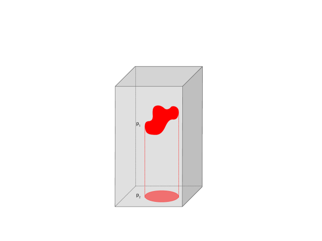
Figure 1: A loop $K$, denoted by $p_{2}$, in the ($x_{1},x_{2}$) plane can be lifted up to form a knot ${\bf K}$, denoted by $p_{1}$, once we go to the Euclidean space. Non-trivial Wilson loop can now be constructed by integrating the twisted gauge field ${\cal A}_{d}$ along the knot $p_{1}$.

Alternatively we can go to Euclidean space where the co-dimension two singularity is a curve in a three-manifold with non-trivial topology. This will be our knot configuration. This means a co-dimension two singularity in four-dimensional space ${\bf V}$ as in (109) will now be of the form:

$${\bf C}\equiv{\bf K}\times{\bf R}_{+},$$ (350)

where ${\bf K}$ is a knot in three-dimensional Euclidean space (not to be confused with the loop $K$ discussed earlier in (345)) and ${\bf R}_{+}$ is our $\psi$ direction. In the equivalent Minkowski space, ${\bf K}$ would be a one-dimensional curve in ($x_{0},x_{1},x_{2}$) plane. In the above discussion of putting a co-dimension two singularity along ($x_{0},\psi,\phi_{1}$) directions the charge of the dual D0-brane bound state (with D6-branes) appears from:

$$\int_{\Sigma_{11}}{\cal C}_{3}\wedge{\cal G}_{4}\wedge{\cal G}_{4}=\int{\cal A}_{0}dx_{0}\int_{\Sigma_{6}}\langle{\cal F}\rangle\wedge\langle{\cal F}\rangle\wedge\langle{\cal F}\rangle\int_{\rm TN}\omega\wedge\omega,$$ (351)

as such this amounts to switching on two extra components of gauge fields $\langle{\cal A}_{1}\rangle$ and $\langle{\cal A}_{\psi}\rangle$ in addition to what we had earlier. The caveat however is that, as discussed above, the temporal loop would vanish if we want to maintain our gauge choice (170) or (187). On the other hand, once we take a curve in the ($x_{0},x_{1},x_{2}$) space, this issue doesn’t arise and knots can arise naturally (see also Fig 1).

In the same vein if we allow the co-dimension two singularity to be along ($x_{0},\psi,r$) directions, then the dual M2-brane state will be along ($x_{0},\phi_{1},r$) directions. Going to the Euclidean space we can allow the co-dimension two singularity to be along ${\bf C}\times{\bf R}$, where ${\bf C}$ is the surface given in (350) and ${\bf R}$ is the radial direction $r$. The dual M2-brane state then would be along ${\bf K}\times{\bf R}\times\phi_{1}$, where ${\bf K}$ is the knot. In the IIA framework this is again an instanton in a four-dimensional space, whose two coordinates are ($x_{3},\psi$) and the other two coordinates are orthogonal to the knot ${\bf K}$.

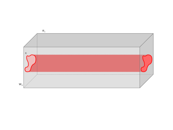
Figure 2: A surface operator constructed out of a M2-brane intersects the three-dimensional Euclidean boundary ${\bf W}$ (or ${\bf W}_{3}$ in the language of [11]) along a knot ${\bf K}$ and is stretched along the remaining $\psi$ direction, which we denote here as ${\bf R}_{+}$. As such it is a co-dimension two singularity both on the three-dimensional boundary ${\bf W}_{3}$ as well as the four-dimensional space ${\bf V}\equiv{\bf W}_{3}\times{\bf R}_{+}$.

Thus for either of the case discussed above, the co-dimensional two singularity in the Euclidean space is identical and is given in Fig 2, although the M-theory uplifts differ. Previously when the co-dimension two singularity was along ($x_{0},x_{1}$) the equations governed by the hypermultiplet scalars (${\cal A}_{2},{\cal A}_{\psi},\varphi_{2},\varphi_{3}$) were the Hitchin’s equations (296) from the BHN equation (293) in the absence of the surface operator; and (3.3.1) from the BHN equation (3.3.1) when the surface operator is present. Now our hypermultiplet scalars would appear from directions orthogonal to the knot ${\bf K}$ therefore the analysis will be different. However if we consider a knot configuration given in Fig 3, away from the neighborhood points $Q_{i}$, we have:

$$\oint_{\bf K}{\cal A}~{}\to~{}\int_{x_{1}}{\cal A}_{1}dx_{1},$$ (352)

then again we expect the local picture to be similar, namely, the Hitchin’s equations (296) get suitably modified like (3.3.1) (although $\sigma$ and $\bar{\sigma}$ in (3.3.1) need to be interpreted carefully now).

We are now getting closer to the approach initiated in the series of papers [32], [33], [36] and [34] and also in [11]. The co-dimension two singularity in Euclidean space that we discuss here is clearly related to the monodromy defect studied in [11] and [36]. Moreover, since we study static configurations (using the Hamiltonian (167)), the temporal direction $x_{0}$ remains suppressed and the co-dimension one singularity in the three-dimensional boundary of our earlier discussions continues to provide accurate description of the singularity structure of the (4, 4) hypermultiplets locally, although the global picture may be different. This shift of our view point from global to local is not just a mere rephrasing of (352) but more of a helpful calculational tool where analysis pertaining to specific knots could at least be addressed. In particular, for the present context, this helps us to channel our earlier computations to analyze non-trivial knot configurations instead of just closed loops discussed in (345).

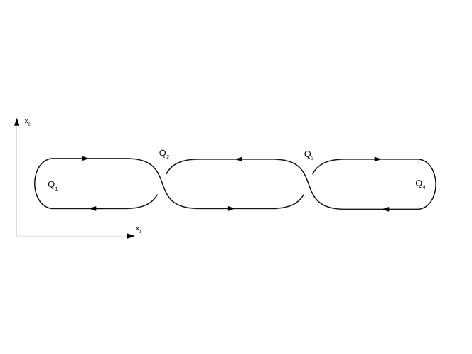
Figure 3: An unknot configuration drawn almost parallel to the $x_{1}$ axis to simplify the computation of the Wilson loop. Thus away from the regions denoted by $Q_{i}$, we can restrict the Wilson line integral to be only along $x_{1}$.

We can make our analysis a bit more precise. In the presence of the knot ${\bf K}$, the part of the boundary three-dimensional action (3.3.1) for the abelian case remains unchanged in form with ${\cal A}_{d}$ defined appropriately with $\hat{\phi}$. The additional piece of the action will be more non-trivial than (344) as now we expect the integral to be over a knot ${\bf K}$. The total action will then take the form similar to (345) with the loop $K$ replaced by the knot ${\bf K}$ and ${\cal A}$ by ${\cal A}_{d}$. For completeness we reproduce this again as:

$$S_{bnd}=(b_{2}+c_{2})\int_{\bf W}{\cal A}_{d}\wedge d{\cal A}_{d}+Q_{2}\oint_{\bf K}{\cal A}_{d},$$ (353)

where $Q_{2}$ can be calculated from M-theory using either the dual D0-brane charge (351), or the dual M2-brane charge depending on our choice of orientation. For the latter case $\hat{\phi}$ in the definition of ${\cal A}_{d}$ will take a different form (that can be determined with some effort, but we will not do so here). Various other details like the field strength ${\cal F}_{d}$ as well as the monodromy around ${\bf K}$ remain similar to (346) and (347) respectively. Furthermore, the presence of ${\cal A}_{d}$ in the integral over the knot ${\bf K}$ can now be directly hinted from (3.3.1) and (3.3.1) by the following replacement:

$${\cal F}_{\alpha\psi}~{}\to~{}{\cal F}_{\alpha\psi}+\langle{\cal F}_{\alpha\psi}\rangle\equiv{\cal F}_{\alpha\psi}+g_{\alpha}{\cal D}_{\psi}\hat{\varphi}_{\alpha},$$ (354)

where $g_{\alpha}$ is an appropriate constant and there is no sum over alpha. Indeed the above defines the gauge field ${\cal A}_{d,\alpha}\equiv{\cal A}_{\alpha}+g_{\alpha}\hat{\varphi}_{\alpha}$ that eventually appears through the boundary magnetic charge ${\bf Q}_{M}$ into the boundary coupling (353). One may easily see that in our earlier derivation this replacement for ${\cal A}_{2}$ was not necessary despite the existence of $\langle{\cal A}_{2}\rangle$ because the instanton configuration therein was defined in the space parametrized by ($x_{2},x_{3},r,\phi_{1}$) and thus independent of the $\psi$ coordinate. However now the dual D0-brane charge (351) does depend on all coordinates orthogonal to the Taub-NUT space and as such (354) becomes necessary.

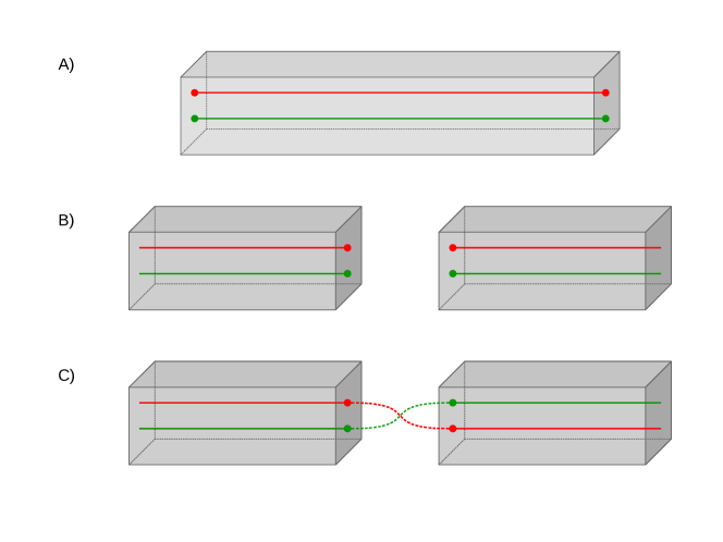
Figure 4: Two Wilson lines in the three-dimensional boundary denoted by (A) is arranged so that they are parallel to the $x_{1}$ axis. In (B) we split them via Heegaard splitting and they are rejoined in (C) via a braid group action. This procedure allows us to introduce non-trivial structures to the Wilson lines.

Our short discussion above shows that, at least for the abelian case, the boundary theory appearing from the magnetic charge ${\bf Q}_{M}$ in the presence of a surface operator does have all the essential properties to study knot configurations. The brief mismatch that we had earlier in the boundary theory (345) goes away once the background is correctly defined as we see in (353). All this is satisfactory and one might, at this stage, even speculate how the non-abelian extension may look like. The non-abelian boundary Chern-Simons theory will have the form (250), but now ${\cal A}_{d,\alpha}$ will have to be defined with respect to $\hat{\phi}_{\alpha}$. The knot will then be added as a linear term in ${\cal A}_{d}$, just as in (353), but now to (250). The above statements are easy to state but a direct derivation of the boundary action along the lines of our earlier discussion is unfortunately harder because of the issues pointed out above. We will therefore relegate a detailed discussion to the sequel of this paper and instead make some generic statements here.

There is one puzzle however that we need to clarify. The non-abelian Chern-Simons theory (250) with the coupling ${k\over 4\pi}\equiv b_{2}+c_{2}$, appearing in (239) and (72), is well defined in a path integral only when $k$ is an integer. With a gauge group $G$, the path integral representation is given by:

$$Z({\bf K},k,G)=\int{\cal D}{\cal A}_{d}~{}{\rm exp}\Big{[}iS_{bnd}(k,{\cal A}_{d})\Big{]}{\rm Tr}_{R}{P}~{}{\rm exp}\left(Q_{2}\oint_{\bf K}{\cal A}_{d}\right),$$ (355)

where the integral is over all gauge connections ${\cal A}_{d}$ modulo gauge transformations. What happens when $k$ is not an integer? This could in general be the case because both $b_{2}$ and $c_{2}$, given in (239) and (72) respectively, appear from supergravity analysis and are as such not restricted to be integers. It turns out, when $k$ is not an integer, we can still perform the path integral by complexifying the gauge field ${\cal A}_{d}$. The story becomes more interesting now, and has been discussed in much details in [37]. This analytical continuation of Chern-Simons theory at the boundary proceeds in few steps: one, to change the measure of the path integral; two, to incorporate the complex conjugate piece in the path integral and then three, to assume the complex conjugate piece, constructed from $\overline{\cal A}_{d}$, to be independent of the one constructed from ${\cal A}_{d}$ [37]. In other words, we change (355) to:

$$Z({\bf K},k,\widetilde{k},G)=\int_{\cal C}{\cal D}{\cal A}_{d}{\cal D}\widetilde{\cal A}_{d}~{}{\rm exp}\Big{[}iS_{bnd}\left(k,{\cal A}_{d}\right)+iS_{bnd}\left(\widetilde{k},\widetilde{\cal A}_{d}\right)\Big{]}{\rm Tr}_{R}{P}~{}{\rm exp}\left(Q_{2}\oint_{\bf K}{\cal A}_{d}\right),$$

where both $\widetilde{\cal A}_{d}$ and $\widetilde{k}$ are in general different from $\overline{\cal A}_{d}$ and $k$ respectively. The choice of the integration cycle ${\cal C}$ is subtle and is captured by finding critical points of the modified Chern-Simons action appearing in (3.3.2) and then expressing ${\cal C}$ in terms of the so-called Lefshetz thimbles [37]. The integrals over these Lefshetz thimbles should always converge, and this way finite values could be determined for the path integral (3.3.2).

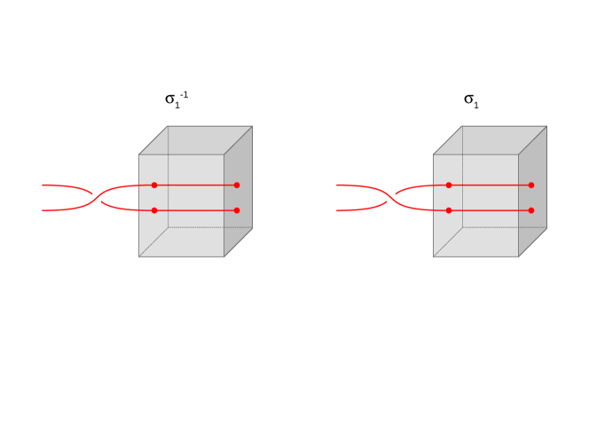
Figure 5: The action of the braid group on the Wilson lines. They are distinguised by their over-crossing and under-crossing pattern. The first one has a braid group action $\sigma_{1}^{-1}$, whereas the second one has a braid group action $\sigma_{1}$.

The above discussion raises an interesting question, namely, what is the interpretation of the above story from our M-theory uplift? To answer this, recall how we arrived at the Chern-Simons theory (250). Our starting point was the four-dimensional action (3.2.10), from where we derived the Hamiltonian (167). The electric and the magnetic charges ${\bf Q}_{E}$ and ${\bf Q}_{M}$ respectively, when arranged properly by taking care of the subtleties mention in section 3.2.12, gave rise to the boundary action (250). There were two crucial ingredients in the discussion: one, the expression (239), which was important in deriving the coupling constant $k$ and two, the twisted gauge field ${\cal A}_{d}$ which in turn was composed of the original gauge field ${\cal A}_{\mu}$ and the twisted scalar field $\phi_{\mu}$. Looking even further back, both the ingredients appeared from M-theory: the twisted gauge field from the G-flux ${\cal G}_{4}$ via (64); and the coupling $k$ (i.e $b_{2}$ and $c_{2}$) essentially from the M-theory action via (71). This means the complexification of the fields that is necessary to analyze (3.3.2) should somehow also appear directly from our M-theory analysis.

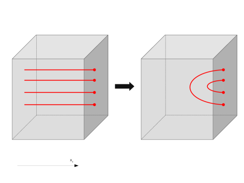
Figure 6: Four Wilson lines are joined pairwise by identifying the respective monodromies around them.

The analysis gets harder because in M-theory, or in the eleven-dimensional supergravity, the ingredients enhancing the four-dimensional gauge theory from abelian to non-abelian and creating the knots may be the same M2-branes. The distinguishing feature is of course their orientations: the non-abelian enhancements appear from M2-branes wrapped on the Taub-NUT two-cycles, whereas the knots appear from M2-branes having at most one leg along the Euclideanized boundary ${\bf W}$ (or being a one-dimensional curve in the three-dimensional Minkowskian boundary). On the other hand when the knot configurations are dual to the D0-branes, with the worldline of the D0-branes forming a knot configuration in the three-dimensional boundary ${\bf W}$, the analysis is equally challenging from M-theory. Even at the abelian level, the essential path-integral that we can lay out is the following:

$$Z(a,b)=\int{\cal D}{\cal G}_{4}~{}{\rm exp}\left[ia\int_{\Sigma_{11}}{\cal G}_{4}\wedge\ast{\cal G}_{4}+ib\int_{\Sigma_{8}}{\cal G}_{4}\wedge{\cal G}_{4}\right]{\rm exp}\left(i\oint{\cal C}_{3}\right).$$ (357)

This is good enough to capture certain aspects of four-dimensional abelian gauge theory as well as the boundary three-dimensional Chern-Simons theory, but definitely not the full story, at least not yet in the present incarnation with $a$ providing the gauge coupling and:

$$b\equiv{c_{2}\over\int_{\rm TN}\omega\wedge\omega},~{}~{}~{}~{}~{}\Sigma_{8}={\bf W}\times{\bf R}_{+}\times{\bf TN},$$ (358)

on the eleven-dimensional manifold $\Sigma_{11}=\Sigma_{8}\times{\bf S}^{3}$, where ${\bf S}^{3}$ is a three-cycle and $\omega$ is the normalizable harmonic form defined on the warped Taub-NUT space. To complete the story, we will need a few crucial intermediate steps: one, that converts $b$ in (357) to $k$ as in (355) via a step similar to (239); two, that converts G-flux ${\cal G}_{4}$ to three-dimensional twisted gauge field ${\cal A}_{d}$; and three, that finally converts (357) to (3.3.2). The search then is a formalism for a topological M-theory where calculations of the kind mentioned above may be performed (somewhat along the lines of [38]).

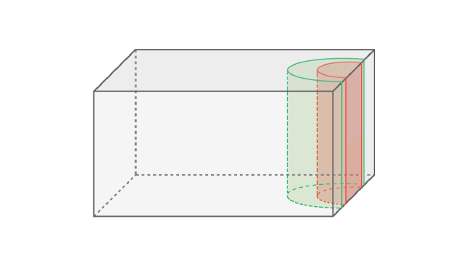
Figure 7: Once we identify monodromies of a pair of Wilson lines, the structure of the co-dimension two surface operator in four-dimensional space can be formed out of two-branes. Here two such configurations are shown on a Heegaard-split three-manifold base.

In the absence of such a formalism, simplification occurs when $k$ becomes an integer, so that we can ignore complexification, and when we go to the abelian case, where we can resort to our earlier calculations. This then brings us to the following path-integral representation:

$$Z({\bf K},k)=\int{\cal D}{\cal A}_{d}~{}{\rm exp}\left({ik\over 4\pi}\int_{\bf W}{\cal A}_{d}\wedge d{\cal A}_{d}\right){\rm exp}\left(iQ_{2}\oint_{\bf K}{\cal A}_{d}\right),$$ (359)

which is simpler than both (355) as well as (3.3.2) and where ${k\over 4\pi}=b_{2}+c_{2}$ is now an integer. Additionally, the quadratic form of the Chern-Simons action implies that (359) can be simplified further. Defining ${\cal A}_{d}=\langle{\cal A}_{d}\rangle+a_{d}$, where $a_{d}$ is the fluctuation over the background field $\langle{\cal A}_{d}\rangle$, and using (346) now for the background field strength $\langle{\cal F}_{d}\rangle$, we can express (359) equivalently as:

$$Z({\bf K},k)=Z_{0}\int{\cal D}{a}_{d}~{}{\rm exp}\left({ik\over 4\pi}\int_{\bf W}{a}_{d}\wedge d{a}_{d}\right),$$ (360)

where $Z_{0}$ is a number and is given by $Z_{0}={\rm exp}\left({ik\over 4\pi}\int_{\bf W}\langle{\cal A}_{d}\rangle\wedge d\langle{\cal A}_{d}\rangle\right){\rm exp}\left(\oint_{\bf K}\langle{\cal A}_{d}\rangle\right)$, implying that the quantum computations in the presence of a knot may be performed by studying the fluctuations over a classical background as if the knot was absent. This simplification is of course only for the abelian case, as the non-abelian case would require more elaboarate computational machinery.

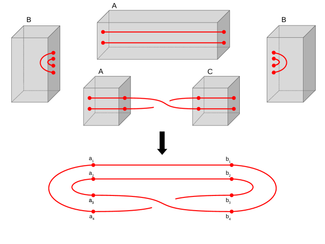
Figure 8: Construction of an unknot using all the ingredients that we developed earlier. Boxes ${\bf A}$ represent the Wilson lines parallel to $x_{1}$ axis, boxes ${\bf B}$ denote the curving of the Wilson lines by identifying pairwise monodromies, and finally box ${\bf C}$ denote the braid group action. Together they form an unknot configuration. The points $a_{i}$ and $b_{i}$ are the points where the Wilson lines end on the Heegaard-split three manifolds.

There is something puzzling about (360) that we would like to clarify. Rephrasing (359) to (360) one might worry that all information about the knot ${\bf K}$ is now lost. In fact what we have in (360) is the following additional integral:

$${\rm exp}\left(-iQ_{2}\int_{\bf W}a_{d}\wedge\delta_{\bf K}\right){\rm exp}\left(iQ_{2}\oint_{\bf K}a_{d}\right),$$ (361)

which vanishes classically and so the computations proceeds as though no knot is present in (360). However (361) imples that the actual quantum mechanical computation should have another knot linked to the previous one. In other words there should be a framing anomaly [2]. Taking this into account, the information about the knot can thus be recovered in the quantum computations.

Let us elaborate this a bit more. For abelian, Chern-Simons, the cubic interaction term is absent. The expectation value of Wilson loop operator for knot $\mathbf{K}$ in (359) can be expressed as:

$$Z({\bf K},k)=\exp\left\{-Q_{2}^{2}\langle\oint_{\mathbf{K}}dx_{\mu}{\cal A}_{d}^{\mu}(x)\oint_{\mathbf{K}}dy_{\nu}{\cal A}_{d}^{\nu}(y)\rangle\right\},$$ (362)

where $Q_{2}$, as mentioned earlier, may be computed in M-theory from the dual D0-brane charge (351) or from dual M2-brane charge depending on our choice of orientation. Using the gauge field two point function:

$$\langle{\cal A}_{d}^{\mu}(x){\cal A}_{d}^{\nu}(y)\rangle=\epsilon^{\mu\nu\lambda}~{}{(x-y)_{\lambda}\over|x-y|},$$ (363)

we see that the above invariant (362) will blow up at coincident points $x_{\mu}\rightarrow y_{\mu}$. So we will have to regularize the integral. This is achieved by choosing a suitable frame with a ${\mathbf{K}_{f}}$ knot slightly displaced from the original knot. In other words, we take the coincident points as $y_{\mu}=x_{\mu}+\epsilon_{\mu}$, with $\epsilon_{\mu}$ approaching zero. Depending on the choice of frame, we will get the $U(1)$ knot invariant (362) to be in terms of a framing number $p$, defined as the linking number of knot ${\mathbf{K}}$ with its frame knot ${\mathbf{K}_{f}}$, in the following way:

$$-{1\over Q_{2}^{2}}~{}{\rm log}~{}Z({\bf K},k)={}^{\rm lim}_{\epsilon_{\mu}\to 0}\langle\oint_{\mathbf{K}}dx_{\mu}{\cal A}_{d}^{\mu}(x)\oint_{\mathbf{K}_{f}}dy_{\nu}{\cal A}_{d}^{\nu}(y)\rangle=-{i\pi p\over k},$$ (364)

implying that for any knot the result is proportional to $p$. However, we can always choose a canonical frame in ${\bf S}^{3}$ where $p=0$. In other words, this canonical frame does not give any information about knots within abelian Chern-Simons theory. This is exactly reflected by perturbing the classical background solution as detailed in (360) and (361). Thus non-trivial information is achieved when we go from one frame to another. For more details see [39].

We are now ready to discuss the construction of knots using our surface operators. One of the crucial ingredient is the Heegaard splitting, which states that a three manifold ${\bf W}$ can be obtained as a connected sum of three manifolds ${\bf W}_{1}$ and ${\bf W}_{2}$ joined along their common boundary ${\bf\Sigma}\equiv\partial{\bf W}$. Thus:

$${\bf W}={\bf W}_{1}\cup_{\bf\Sigma}{\bf W}_{2}.$$ (365)

In the presence of a surface operator, a three manifold can also be split in a similar way as depicted in Fig 4, ($A$) and ($B$). Once we extend the Wilson lines along the ${\bf R}_{+}$ direction (or alternatively the $\psi$ direction) in Fig 4($B$), we can see how the surface operators split. The way we have expressed the surface operators, they are parallel to $x_{1}$ axis as can be seen from the Wilson line representation (352). This means on the boundary ${\bf\Sigma}$ of our three manifold ${\bf W}$ the Wilson lines will end on points, and the splitting of the surface operators would imply how the points are distributed on different boundaries. In a standard quantization of the Chern-Simons theory on ${\bf W}$, where ${\bf W}$ is locally a product of ${\bf\Sigma}\times{\bf R}_{1}$ with ${\bf R}_{1}$ representing the direction $x_{1}$, the Hilbert space ${\cal H}_{\bf\Sigma}$ associated to the boundary ${\bf\Sigma}$ changes, in the presence of the surface operator, to:

$${\cal H}_{\bf\Sigma}~{}\to~{}{\cal H}_{{\bf\Sigma};p_{i};R_{i}},$$ (366)

where $p_{i}$ are the points on ${\bf\Sigma}$ where the Wilson lines end and $R_{i}$ are the representations of each points. In the present case the Hilbert space is precisely the gauge theory described on the D2-brane surface operator that we use here.

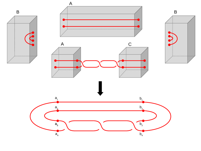
Figure 9: Construction of a trefoil knot by joining boxes ${\bf A}$, ${\bf B}$ and ${\bf C}$ appropriately. The braid group action now acts twice. The points ($a_{i},b_{i}$) still remain the points where the Wilson lines end on the Heegaard-split manifolds.

The next ingredient is the monodromy around the surface operator. We already described the case when we have a loop $K$ in the ($x_{1},x_{2}$) plane for the surface operator given in Table 5. The monodromy therein was given by (347), which can be re-expressed in the language of ($\alpha,\beta,\gamma$) using the BHN equations (317), where ($\alpha,\beta,\gamma$) have in-turn been expressed using supergravity variables in (3.3.1) and (319). In eq. (6.4) of [11], and also in eq. (2.2) and eq. (2.3) of [33] with more details, the gauge field ${\cal A}$ and the scalar field $\hat{\phi}$ have been described using ($\alpha,\beta,\gamma$). Using (3.3.1) and (319), we now express (${\cal A},\hat{\phi}$) using supergravity variables. This is no surprise, of course, as in our earlier sections we used supergravity to write the BHN equations for ${\cal F}_{\alpha\beta}$ and ${\cal F}_{\alpha\psi}$. Thus the monodromy around the $k$-th surface operator (347) can be now written as:

$${\cal M}_{k}\equiv{\rm exp}\left[-2\pi(\alpha_{k}-i\gamma_{k})\right].$$ (367)

Since a given surface operator is a solution of the set of equations (3.3.1), (335), (3.3.1), (333) and (334), monodromies around different surface operators depend on their respective choices of the triplets ($\alpha_{k},\beta_{k},\gamma_{k}$).

The gauge field set (${\cal A},\hat{\phi}$) that we take appears in the boundary Chern-Simons theory as a combined gauge field ${\cal A}_{d}$ as defined in (249) and in (3.3.1). There are three parameters that appear in the definition of ${\cal A}_{d}$: $b_{2}$ and $c_{2}$ from gauge theory coupling constant (239) after twisting, and $d_{1}$ from (241). It is easy to see that although $b_{2}$ and $c_{2}$ both have to be real, $d_{1}$ can in principle be complex. Nothing that we discussed earlier will modify if $d_{1}$ becomes a complex function. In fact there are two ways to go about this, with definite advantages in either formalism. Using ${\cal A}_{\mu}=-iA_{\mu}$ as in (3.3.1), we can express ${\cal A}_{d}$ as:

$${\cal A}_{d}~{}=~{}-i\left(A-{id_{1}\over b_{2}+c_{2}}\hat{\phi}\right),$$ (368)

which keeps $d_{1}$ real, but inserts an $i$ in the definition of the gauge field. In this formalism, a boundary flat connection implies a Hitchin equation of the following form:

$$d{\cal A}_{d}-i{\cal A}_{d}\wedge{\cal A}_{d}~{}=~{}0~{}=~{}F+\left({d_{1}\over b_{2}+c_{2}}\right)^{2}\hat{\phi}\wedge\hat{\phi},$$ (369)

where note the relative plus sign. Comparing this with say (335), which is expressed in variables before twisting, we see that they are similar provided we use ${\cal F}_{12}=-iF_{12}$ as in (3.3.1). After twising the coefficients of (369) may be identified with the ones in (335) and this way the value of $d_{1}$ may be determined.

In the second formalism, we keep the gauge field as ${\cal A}_{\mu}$, but make $d_{1}$ itself complex. If we now map all the variables in the action (3.2.10) to the ones appearing in say [11] using ($\sigma_{0},\gamma_{0},\kappa_{0}$) etc in (220) and (224) respectively, then one can show that:

$$d_{1}~{}\equiv~{}\pm{ic_{11}(b_{2}+c_{2})\over\sqrt{c_{11}^{2}+v_{3}^{2}q^{2}~{}{\rm sin}^{2}\theta}},$$ (370)

where $c_{11}$ is given in (85), $v_{3}$ in (75) and $q(\theta)$ in (76) with a NC deformation $\theta$. This definition of $d_{1}$ doesn’t change if we change $\phi$, in the absence of a surface operator, to $\hat{\phi}$, in the presence of one. Additionally it is interesting to note that there are certain values of the NC parameter $\theta$ for which the definition of the boundary gauge field ${\cal A}_{d}$ simplifies to:

$${\cal A}_{d}={\cal A}\pm i\hat{\phi}.$$ (371)

The simplest case is of course when $\theta$ vanishes. The other case may arise when $q(\theta)$, as defined in (259), vanishes for non-zero $\theta$. Clearly for all these cases $c_{2}$ also vanishes, and $t$ becomes $t=\pm i$. However the boundary gauge theory coupling continues to remain non-zero and now takes the value $b_{2}$ as can be seen from (239).

Unfortunately, as it turns out, by doing similar mapping of our variables to the ones in [11] as discussed above, $b_{2}$ becomes infinite when $t$ approaches $\pm i$. In this limit, and as elaborated in [12], $\tau$ defined in (192) becomes irrelevant and therfore is not an useful arena to study the boundary theory. Thus it seems we should only allow $t\neq\pm i$ cases, which then brings us to the question whether the simplification (371) is any way useful for us.

A path integral representation sheds some light here. Let us first discuss the non-abelian case in the absence of any knots. The path integral can be written as:

$$\int_{\cal C}{\cal D}{\cal A}_{d}~{}{\rm exp}\Bigg{[}i(b_{2}+c_{2})\int_{\bf W}{\rm Tr}\left({\cal A}_{d}\wedge d{\cal A}_{d}+{2i\over 3}{\cal A}_{d}\wedge{\cal A}_{d}\wedge{\cal A}_{d}\right)\Bigg{]},$$ (372)

where ${\cal C}$ is the same integration cycle that we discussed earlier; and we see that (372) only depends on the combination $b_{2}+c_{2}$ but does not depend on the ratio ${d_{1}\over b_{2}+c_{2}}$, which is another way of saying that ${\cal A}_{d}$ is a dummy variable in the integral (372). We can therefore replace ${\cal A}_{d}$ by any complex function and the definition (371) would equally suffice if we view ${\cal A}$ and $\hat{\phi}$ to be arbitrary functions appearing in the path integral. All in all, it boils down to the fact that the gauge field appearing in the path integral may be an arbitrary complex one-form, although the boundary action is defined with a specific functional form for ${\cal A}_{d}$. Even in the presence of a knot, for both abelian and non-abelian cases, the arguments presented above go through because the Wilson loop is defined with ${\cal A}_{d}$, and as such could again be replaced by an arbitrary complex one-form in the path integral. All these observations resonate well with the ones presented in sec (2.4) of [11].

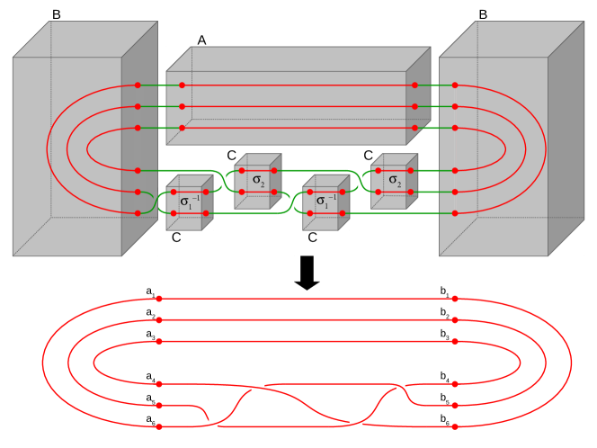
Figure 11: The construction of a figure 8 knot using ${\bf A}$, ${\bf B}$ and ${\bf C}$ boxes in a slightly different way than discussed earlier. The braid group action is now $\sigma_{1}^{-1}\cdot\sigma_{2}\cdot\sigma_{1}^{-1}\cdot\sigma_{2}$ acting on the Wilson lines as shown.

Further simplification occurs when we look at the BHN equations (3.3.1) and (335) on a plane orthogonal to the surface operator. Since $\sigma$, as well as its covariant derivatives (326) and (337), are localized functions we expect the behavior in a plane away from the center of the surface operator to be:

$${\cal F}_{1\psi}-i\gamma_{4}\left[\varphi_{1},\varphi_{3}\right]~{}=~{}{\cal F}_{2\psi}-i\gamma_{4}\left[\varphi_{2},\varphi_{3}\right]~{}=~{}{\cal F}_{12}-i\gamma_{7}\left[\varphi_{1},\varphi_{2}\right]~{}=~{}0,$$ (373)

where $\gamma_{7}$ is the coefficient of the commutator piece in (335). Note that we have expressed the BHN equations without the hats, as the $\sigma$ dependences die off in the orthogonal plane. Converting the gauge fields from ${\cal A}_{\mu}$ to $-iA_{\mu}$ using (3.3.1), the Hitchin equation for ${\cal F}_{12}$ in (373) match with (369) as noted earlier. Of course the above discussion is good only for the configuration that we study in Table 5 which is a co-dimension one singularity in the three-dimensional boundary. For a co-dimension two singularity in the boundary, we will have to study the Hitchin’s equations in a plane orthogonal to the surface operator. The analysis would be similar to what we did above, although certain specific details might be different now.

The picture that we developed above leads to the concept of holonomy of the complex gauge field around a given surface operator. This can typically be represented by $V_{k}\equiv{\rm Hol}({\cal A}_{d(k)})$ with $k$ representing the $k$-th surface operator. For flat connections holonomy and monodromy are related so $V_{k}$ will be conjugate to the monodromy ${\cal M}_{k}$ in (367). An interesting consequence of having holonomy around a surface operator is the following. Consider four Wilson lines parallel to each other and intersecting at four-points on $\Sigma$ in a Heegaard split three-manifold. This is depicted to the left of Fig 6, where the Wilson lines are parallel to $x_{1}$ direction. If we name them as 1, 2, 3 and 4, then by identifying the monodromies:

$${\cal M}_{1}={\cal M}_{4}^{-1},~{}~{}~{}~{}~{}~{}~{}~{}~{}{\cal M}_{2}={\cal M}_{3}^{-1},$$ (374)

or equivalently the holonomies, we can go to the configuration depicted to the right of Fig 6. This operation is useful because it tells us that we can join two Wilson lines by identifying monodromies. In terms of surface operators, this procedure will lead to the configuration depicted in Fig 7.

In fact we now have two distinct configurations of Wilson lines, or equivalently, surface operators. The first one, we will call it box A and is depicted in Fig 4 (A), is a configuration of parallel surface operators. The second one, and we will call it box B, is depicted to the right of Fig 6: a configuration of curved surface operators. Associated to these boxes will be the operators ${\bf A}_{k}$ and ${\bf B}_{k}$ where $k$ denote the number of surface operators (or equivalently, Wilson lines).

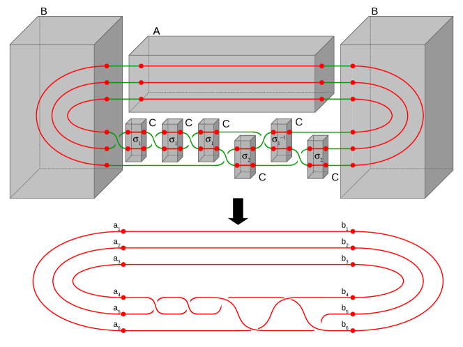
Figure 12: The construction of $5_{2}$ knot using the ${\bf A}$, ${\bf B}$ and ${\bf C}$ boxes. The braid group action is now $\sigma_{1}^{3}\cdot\sigma_{2}\cdot\sigma_{1}^{-1}\cdot\sigma_{2}$ acting on the Wilson lines as shown.

There is a third possibility that we can entertain and is depicted in Fig 4 (C). We will call it box C, where the Wilson lines are swapped by a braid group action $\sigma_{\alpha}$. We will concentrate on a braid group with two strands, with generators $\sigma_{\alpha}$ where the subscript $\alpha$ denote which set of two strands, out of a given set of Wilson lines, we choose here. The operators associated with the braid group action will be ${\bf C}_{(2,\sigma_{1})}$ and ${\bf C}_{(2,\sigma^{-1}_{1})}$ where we take $\alpha=1$ for illustrative purpose and the two operations are depicted in Fig 5. We therefore expect:

$${\bf C}_{(2,\sigma_{1})}{\bf C}_{(2,\sigma^{-1}_{1})}~{}=~{}{\bf C}_{(2,1)},$$ (375)

where $\sigma_{1}=1$ implies no braid group action. This is therefore topologically equivalent to ${\bf A}^{\intercal}_{2}$, with transpose put in to account for the orientations of the Wilson lines.

We now have more or less all the necessary ingredients to analyze the invariants for various knots. Let us start with the simplest case of an unknot as depicted in Fig 8. Combining the boxes ${\bf A}$, ${\bf B}$ and ${\bf C}$ we can express the invariant (or the linking number) in the following way:

$$Z(q;~{}{\bf K}_{0})~{}=~{}\langle{\rm exp}\oint_{{\bf K}_{0}}{\cal A}_{d}\rangle~{}=~{}\sum_{n_{2}}\langle n_{2}|{\bf B}_{2}^{\intercal}{\bf C}_{(2,\sigma_{1})}{\bf B}_{2}{\bf A}_{2}|n_{2}\rangle,$$ (376)

where ${\cal A}_{d}$, as described above, could be any complex one-form; and ${\bf K}_{0}$ is the unknot configuration. The action of the operators in the RHS of (376) can be elaborated in the following way. Consider box ${\bf A}$ in Fig 8 where the Wilson lines intersect the top right two-dimensional surface $\Sigma$ at two points. These two points may be considered as a given state $|n_{2}\rangle$ in the boundary $U(1)$ Chern-Simons theory. The operator ${\bf A}_{2}$ evolves the state from right to left (here we take the direction to be parallel to $x_{1}$, but this is not necessary). The subscript $2$ denotes two strands (or the two particle state $|n_{2}\rangle$) in the field theory. The operator ${\bf B}_{2}$ then curves the Wilson-line states by monodromy identification, much like (374) discussed above. This evolution continues till the braid group operation ${\bf C}_{(2,\sigma_{1})}$ acts in the way depicted in Fig 8. The braided state is then evolved by ${\bf B}_{2}^{\intercal}$ where the transpose operation just reverses the orientations of ${\bf B}_{2}$. Finally we sum over all possible two Wilson-line states in the Chern-Simons theory.

The above, slightly unconventional way, reproduces the invaraint (362) for the unknot case using the operators ${\bf A}_{2}$, ${\bf B}_{2}$ and ${\bf C}_{(2,\sigma_{1})}$ combined as (376). All the three operators can be thought of as a $2\times 2$ matrices whose components are evolution operators. As such they are expressible in terms of exponentials of generators integrated over the knot configuration, exactly as in (362). This can be normalized to 1, so one might wonder why we went about expressing the unknot in a rather complicated way. The answer is that the above way of expressing the unknot using the operators, help us to generalize the picture to any complicated torus knots. For example, let us consider the trefoil depicted in Fig 9, which again uses the three set of operators ${\bf A}_{2}$, ${\bf B}_{2}$ and ${\bf C}_{(2,\sigma_{1})}$. The knot invariant associated with the trefoil then is:

$$Z(q;~{}{\bf K}_{t})~{}=~{}\langle{\rm exp}\oint_{{\bf K}_{t}}{\cal A}_{d}\rangle~{}=~{}\sum_{n_{2}}\langle n_{2}|{\bf B}_{2}^{\intercal}{\bf C}_{(2,\sigma_{1})}{\bf C}_{(2,\sigma_{1})}{\bf C}_{(2,\sigma_{1})}{\bf B}_{2}{\bf A}_{2}|n_{2}\rangle,$$ (377)

where ${\bf K}_{t}$ denotes the trefoil knot. The operators act in the same way as in (376), except now we have three times the braid group action by the operator ${\bf C}_{(2,\sigma_{1})}$. This of course distinguishes it from (376), and thus the above analysis generalizes easily to the torus knots ($2,n$) as:

$$Z(q;~{}{\bf K}_{\intercal})~{}=~{}\langle{\rm exp}\oint_{{\bf K}_{\intercal}}{\cal A}_{d}\rangle~{}=~{}\sum_{n_{2}}\langle n_{2}|{\bf B}_{2}^{\intercal}{\bf C}^{n}_{(2,\sigma_{1})}{\bf B}_{2}{\bf A}_{2}|n_{2}\rangle,$$ (378)

with ${\bf K}_{\intercal}$ representing the torus ($2,n$) knots. Clearly when $n=3$ we get our trefoil invariant.

So far we have been using the operator ${\bf C}_{(2,\sigma_{1})}$ to represent the braid group action for two Wilson lines. The question is what happens when we have more than two Wilson lines. It turns out we can still use ${\bf C}_{(2,\sigma_{1})}$ but represent the braid group action is a slightly different way. An example of this can be presented for the figure 8 knot, which is the simplest non-torus knot, given in Fig 11. The knot invariant for this is now:

$$Z(q;~{}{\bf K}_{8})~{}=~{}\langle{\rm exp}\oint_{{\bf K}_{8}}{\cal A}_{d}\rangle~{}=~{}\sum_{n_{3}}\langle n_{3}|{\bf B}_{3}^{\intercal}{\bf C}^{m_{{}_{1}}}_{(2,\sigma_{2})}{\bf C}^{m_{{}_{2}}}_{(2,\sigma^{-1}_{1})}{\bf C}^{m_{{}_{3}}}_{(2,\sigma_{2})}{\bf C}^{m_{{}_{4}}}_{(2,\sigma^{-1}_{1})}{\bf B}_{3}{\bf A}_{3}|n_{3}\rangle,$$

where ${\bf K}_{8}$ is the figure 8 knot with $m_{1}=m_{2}=m_{3}=m_{4}=1$; and ${\bf C}_{(2,\sigma_{2})}$ and ${\bf C}_{(2,\sigma^{-1}_{1})}$ are the braid group actions ($\sigma_{1},\sigma_{2}$) on two different strands. The inverse to be understood as the operations depicted in Fig 5. The rest of the operators act in the way we described earlier. We can generalize (3.3.2) by considering arbitrary values for $n_{i}$ in (3.3.2). One such generalization leads to the $5_{2}$ knot given in Fig 12, whose knot invariant may be written as:

$$Z(q;~{}{\bf K}_{5_{{}_{2}}})~{}=~{}\langle{\rm exp}\oint_{{\bf K}_{5_{{}_{2}}}}{\cal A}_{d}\rangle~{}=~{}\sum_{n_{3}}\langle n_{3}|{\bf B}_{3}^{\intercal}{\bf C}_{(2,\sigma_{2})}{\bf C}_{(2,\sigma^{-1}_{1})}{\bf C}_{(2,\sigma_{2})}{\bf C}^{3}_{(2,\sigma_{1})}{\bf B}_{3}{\bf A}_{3}|n_{3}\rangle,$$

where ${\bf K}_{5_{{}_{2}}}$ is the $5_{2}$ knot, and we have taken ${\bf C}^{3}_{(2,\sigma_{1})}$ instead of ${\bf C}^{3}_{(2,\sigma^{-1}_{1})}$ action. We thus see that the three ingredients, namely (a) the Heegaard splittings, that typically lead to a class of operators ${\bf A}_{k}$; (b) Monodromy identifications, that lead to a class of operators ${\bf B}_{k}$; and (c) braid group actions that lead to a class of operators ${\bf C}_{(2,\sigma_{\alpha})}$ and ${\bf C}_{(2,\sigma^{-1}_{\alpha})}$ are sufficient to give us both the surface operator representations as well as the invariants for any given knots. All these are expressible in the language of a $U(1)$ Chern-Simons theory with a complex gauge group ${\cal A}_{d}$ and the invariants that we computed above are proportional to:

$$\exp\left({i\pi p~{}Q_{2}^{2}\over k}\right),$$ (381)

which are consistent with the generic argument that we presented for (362). This is not a big surprise, and one might wonder if we can get anything more out of our elaborate constructions beyond the expected result (381). The answer turns out to be affirmative and in fact accommodates the polynomial constructions outlined in [36] where the monodromies ${\cal M}_{k}$ in (367) are used to construct the variables ($\theta_{i}$, $x_{i}$) and the affine cubic $f(x_{i},\theta_{m})=0$ (see for example equations (4.6), (4.7) and (4.9) of [36]). This means the surface operator representations presented for various knot configurations above not only give us the knot invariants, but also reproduce all the constructions of [36]. Additionally, our analysis shows that all the constructions of [36] may be given a supergravity interpretation!

However once we go to the non-abelian extension, we face many issues, and the simple minded analysis that we presented here will have to be modified. This means, for example, a surface operator representations of Jones polynomials using the three kinds of operators we used here are not sufficient. A more detailed framework is then called for, which is unfortunately beyond the scope of the present work. We will therefore not discuss this further, instead we will elaborate on another set of constructions that generalize easily to the non-abelian case.

3.3.3 ’t Hooft operator, opers and supergravity parameters

In the previous section we have considered the co-dimension two defect operators in the field theory. The monodromy defect supported on a knot ${\bf K}$ inside the Chern-Simons boundary was extended in four dimensions to a singularity that the fields had along a two dimensional surface ${\bf K}\times{\bf R}_{+}$ inside the four dimensional space.

In [11] and [13], other defect operators were considered in a four dimensional theory, the co-dimension one Wilson line operators and the co-dimension three ’t Hooft operators. Especially important are the co-dimension three ’t Hooft operators which can be related to the Nahm pole solution where the dependence of the co-dimension three object is only on $\psi$, the four dimensional coordinate transversal to the three dimensional boundary. The relevant equations have already appeared in (194), which are of course the ones of [11]. Note that, compared to our earlier sections, nothing we say in this subsection will be new. However an attempt will be made to pave a way for possible connections between the results of [13] and our supergravity analysis.

Let us first consider $t=1$ case, where $t$ is given, in our language of supergravity, by (193). In this case, a stationary solution (invariant under translations along time direction) with zero $A_{\mu}$ and $\phi_{3}$ reduce to Nahm’s equations for the components of the field $\phi$ tangent to the boundary:

$$\frac{d\overrightarrow{\phi}}{dy}+\overrightarrow{\phi}\times\overrightarrow{\phi}=0,$$ (382)

where we have identified $y$ as our $\psi$ coordinate. The above equation follows easily from our BHN equation (3.2.11), and also from (335) which is in the presence of a surface operator provided we change $\phi$ to $\hat{\phi}$. In the language of commutator brackets of (3.2.11) or (335), it is not too hard to guess the solution of the above equation to be:

$$\overrightarrow{\phi}=\frac{\overrightarrow{\tau}}{y},$$ (383)

where $\tau_{a}$ are the three Pauli matrices. The advantage of expressing the equations in terms of three-dimensional vectors, before twisting, allows us to compare with the equations after twisting when they all become one-forms.

Once $A_{\mu}$’s are non-vanishing, the scenario is not so simple as the Nahm equation (382). From our earlier analysis, we know that we need the full BHN equations. Of course, as expected, the solutions to the BHN equation again cannot be as simple as (383). It turns out, there are two types of solutions to the BHN equations which may be succintly presented in terms of a complex coordinate $z$ defined as $z=x_{1}+ix_{2}$ (recall that our four-dimensional space is parametrized by ($x_{0},x_{1},x_{2},\psi$) where we already identified $y$ with $\psi$). The first type of solutions are independent of $z$ coordinate. Defining:

$$D_{1}\equiv\frac{\partial}{\partial x_{1}}+i\frac{\partial}{\partial x_{2}}+\left[A_{1}+iA_{2},~{}.\right]$$

$$D_{2}\equiv\frac{\partial}{\partial y}+\left[A_{y}-i\phi_{0},~{}.\right],~{}~{}D_{3}\equiv\left[\phi_{1}-i\phi_{2},~{}.\right],$$ (384)

where $A_{y}\equiv A_{\psi}$; and as mentioned earlier, depending on the mapping (165) or (291), we can identify $\phi_{0}$ to either ${\cal A}_{3}$ or $\varphi_{3}$ respectively. This means, for certain choice of the gauge ((170) or (187)), $\phi_{0}$ may vanish and therefore $D_{2}$ described above may be simplified. However for the present discussion, we will keep things generic. The first order differential operators $D_{i}$ therefore satisfy:

$$\left[D_{i},D_{j}\right]=0,~{}~{}i,j=1,2,3;~{}~{}~{}~{}~{}~{}~{}~{}~{}~{}~{}\sum_{i=1}^{3}\left[D_{i},D^{\dagger}_{i}\right]=0,$$ (385)

which are alternative ways to express the BHN equation (217) or (3.2.11) once we absorb some factors and signs appropriately. To verify that this is indeed, for example, (217) we note that the second equation in (385) is the moment map equation which can be written as:

$$F_{12}-\left[\phi_{1},\phi_{2}\right]-D_{y}\phi_{0}=0.$$ (386)

In the gauge $A_{1}+iA_{2}=0$, the operator $D_{1}$ becomes derivative with respect to $\bar{z}$ and with the gauge choice $A_{y}=i\phi_{0}$, the operator $D_{2}$ becomes derivative with respect to $y$. $D_{3}$ is proportional to $\phi\equiv\phi_{1}-i\phi_{2}$ as should be clear from (3.3.3). The commutation relation $[D_{1},D_{3}]=0$ implies that $\phi$ is holomorphic in $z$ and the relation $[D_{2},D_{3}]=0$ means that $\phi$ is independent of $y$. Near $y=0$, $\phi$ is a constant and a complex valued gauge transformation maps it into the Nahm pole solution with $\frac{1}{y}$ dependence.

What about outside the region $y=0$? The vanishing of the commutator brackets $[D_{1},D_{3}]$ and $[D_{2},D_{3}]$ define a Higgs bundle $(E,\phi)$ where $\phi$ is independent of $y$ and holomorphic. The Nahm pole solution (also called the model solution) is trusted around the $y=0$ boundary but we can extend the model solution as a Higgs bundle $(E,\phi)$ away from $y=0$. In fact, as described in [13], such extension gives a Higgs bundle $(E,\phi)$ endowed with a holomorphic line sub-bundle $L$ which is not stabilised by $\phi$. In other words, for any section $s$ of $L$ we expect $s\wedge\phi s\neq 0$, as described in [13].

Let us now consider the second type of solutions that depend on $z$. The dependence on $z$ is determined by the presence of extra monopoles with extra charges $k_{a}$ at points $z=z_{a}$. Next to $y=0$, the solution is a simple modification of the Nahm pole solution as the field $\phi$ has a holomorphic entry with a power of $z$. Away from $y=0$ the solution is given again by a triplet $(E,\phi,L)$ of a Higgs bundle with a holomorphic sub-bundle $L$.

How do we now extend this result to the case $t\neq 1$? A key observation of [13] is that the Higgs bundle (with the key ingredient of a holomorphic scalar field $\phi$) can be obtained by starting from a set of Hitchin equations:

$$F-\phi\wedge\phi=0;~{}~{}~{}~{}d*\phi=d\phi=0,$$ (387)

and combining the last two equations to get the holomorphicity condition on $\phi$, namely $\bar{\partial}\phi=0$. This is true for $t=1$. When $t\neq 1$, it is useful to modify the definition of the derivatives with respect to $z,\bar{z}$ by introducing a complex parameter $\zeta$ in the following way:

$$D_{z}^{\zeta}=\frac{D}{Dz}-\zeta^{-1}\left[\phi,~{}.\right],~{}~{}~{}~{}~{}D_{\bar{z}}^{\zeta}=\frac{D}{D\bar{z}}+\zeta\left[\bar{\phi},~{}.\right].$$ (388)

We have $[D_{z}^{\zeta},D_{\bar{z}}^{\zeta}]=0$ which is taken as an equation governing holomorphic data. In fact using vector field components $A_{z}^{\zeta}=A_{z}-\zeta^{-1}\phi$ and $A_{\bar{z}}^{\zeta}=A_{\bar{z}}+\zeta\bar{\phi}$ makes (388) holomorphic in these variables. Additionally, the holomorphicity condition on $\phi$ is mapped into a holomorphicity condition on $A_{z}^{\zeta}$ and the Higgs bundle condition is now replaced by a complex flat connection. The Nahm pole solution around $y=0$ now describes a singularity in $A_{z}^{\zeta}$ and $A_{y}$. Away from $y\rightarrow 0$ region, the solution is a complex flat bundle $E$ with a holomorphic bundle $L$ defined such that its holomorphic sections are not annihilated by $D_{z}$. Such a pair $(E,L)$ is called an oper [13].

In the Appendix A of [13], the reduction of a four dimensional stationary solution to a topological theory in three dimensions was a function of a rotational angle $\theta$ where the parameter $t$ was set to ${\rm tan}\left({3\theta\over 2}+{\pi\over 4}\right)$ and $\zeta$ to ${\rm tan}~{}\theta$. This relation between $t$ and $\zeta$ should also appear from our M-theory reduction. As $t$ is related to the supergravity parameters via (193), we expect $\zeta$ to also be represented by our supergravity parameter. From here we conclude that the oper solution is automatically fixed once we have determined the supergravity parameters. This is somewhat along the lines of the discussion in the previous subsections where we saw that many of the results discussed in [11] automatically appear from our supergravity analysis. More details on this will be presented in the sequel to this paper.

4 Model B: The type IIB dual description and non-K$\ddot{a}$hler resolved cone

In section 3 most of our analysis revolved around the uplift of the brane configuration given in Table 1 to M-theory, and the subsequent physics associated to the presence of a knot in $2+1$ dimensional boundary ${\bf W}$. The existence of a Coulomb branch, as well as dipole (or RR) deformation, helped us to study the knots and their localization to the boundary ${\bf W}$. Many of the details, that were studied exclusively from the boundary point of view in [11], appeared very naturally in our set-up from the bulk dynamics in M-theory. The starting point of all our discussion was the Hamiltonian (167) from where, and in the presence of surface operators, we were led to the detailed study of knots and knots invariants.

At this stage it is interesting to ask if we can repeat the success using the second brane configuration given in Table 2. One immediate difference from the earlier brane configuration in Table 1 (or its T-dual type IIA version) is the absence of the Coulomb branch. Recall that the existence of the Coulomb branch earlier was responsible in constructing the twisted gauge field ${\cal A}_{d}$ in (249) which eventually led us to the boundary Chern-Simons theory (250). Once we lose the Coulomb branch, restricting the knot to the three-dimensional boundary ${\bf W}$ is more subtle. In fact the whole boundary picture developed from four-dimensional space ${\bf V}={\bf W}\times{\bf R}^{+}$ a la [11] will need to be re-interpreted differently now. Problems lie in restricting the knots to three-dimensions, constructing the twisted gauge field and resolving the conundrum addressed earlier in section 2.2.

We will start by discussing, in series of steps, a way out of the conundrum for Model B by analyzing the picture from M-theory in a slightly different way from what is discussed in section 5 of [11]. In the process we will get some understanding how to address the other two issues namely, restricting knots to 3d and topological twisting of the scalar fields. But we make only the barest beginnings in this direction, and leave most of the details for the sequel.

4.1 Second look at the gravity and the topological gauge theory

We saw, from our earlier discussion in section 2.2, that an appropriate duality to the brane configuration of Model B leads to a type IIB picture with wrapped D5-branes on the two-cycle of a resolved conifold. According to [40] the metric on the resolved conifold should be non-Kähler. Ignoring the dipole deformation for the time being (we will insert this soon), the supergravity background for the configuration is given by (3.1) as before with $\phi$ being the dilaton and the Hodge star and the fundamental form $J$ are wrt to the dilaton deformed metric $e^{2\phi}ds_{2}^{6}$. The metric $ds_{6}^{2}$ is now different from (14) as its a non-Kähler resolved conifold metric written as:

$$ds^{2}_{6}=F_{1}~{}dr^{2}+F_{2}(d\psi+{\rm cos}~{}\theta_{1}d\phi_{1}+{\rm cos}~{}\theta_{2}d\phi_{2})^{2}+\sum_{i=1}^{2}F_{2+i}(d\theta_{i}^{2}+{\rm sin}^{2}\theta_{i}d\phi_{i}^{2}),$$

where $F_{i}(r)$ are warp factors that are functions of the radial coordinate $r$ only. The above background (4.1) can be easily converted to a background with both ${\cal H}_{3}$ and ${\cal F}_{3}$ fluxes by a series of duality specified in [41, 40]. The duality converts (4.1) to:

$$ds^{2}={1\over e^{2\phi/3}\sqrt{e^{2\phi/3}+\Delta}}~{}ds^{2}_{0123}+e^{2\phi/3}\sqrt{e^{2\phi/3}+\Delta}~{}ds^{2}_{6}$$ (390)

$${\cal F}_{3}=-e^{2\phi}{\rm cosh}~{}\beta\sqrt{F_{2}\over F_{1}}\left(g_{1}~{}e_{\psi}\wedge e_{\theta_{1}}\wedge e_{\phi_{1}}+g_{2}~{}e_{\psi}\wedge e_{\theta_{2}}\wedge e_{\phi_{2}}\right)$$

$${\widetilde{\cal F}}_{5}=-{\rm sinh}~{}\beta~{}{\rm cosh}~{}\beta\left(1+\ast_{10}\right){\cal C}_{5}(r)~{}d\psi\wedge\prod_{i=1}^{2}~{}{\rm sin}~{}\theta_{i}~{}d\theta_{i}\wedge d\phi_{i}$$

$${\cal H}_{3}={\rm sinh}~{}\beta\Big{[}\left(\sqrt{F_{1}F_{2}}-F_{3r}\right)e_{r}\wedge e_{\theta_{1}}\wedge e_{\phi_{1}}+\left(\sqrt{F_{1}F_{2}}-F_{4r}\right)e_{r}\wedge e_{\theta_{2}}\wedge e_{\phi_{2}}\Big{]}$$

with a dilaton $e^{\phi_{B}}=e^{-\phi}$ and a $\Delta$ defined as:

$$\Delta={\rm sinh}^{2}\beta\left(e^{2\phi/3}-e^{-4\phi/3}\right)$$ (391)

and $\beta$ is a parameter related to certain boost that is explained in [40] while the others, namely ($g_{1},g_{2},{\cal C}_{5}$) are given by:

$$g_{1}(r)=F_{3}\left(\sqrt{F_{1}F_{2}}-F_{4r}\over F_{4}\right),~{}~{}~{}g_{2}(r)=F_{4}\left(\sqrt{F_{1}F_{2}}-F_{3r}\over F_{3}\right)$$ (392)

$${\cal C}_{5}(r)=\int^{r}~{}{e^{2\phi}F_{3}F_{4}\sqrt{F_{1}F_{2}}\over F_{1}}\left[\left({\sqrt{F_{1}F_{2}}-F_{3r}\over F_{3}}\right)^{2}+\left({\sqrt{F_{1}F_{2}}-F_{4r}\over F_{4}}\right)^{2}\right]dr.$$

4.1.1 Revisiting the topologically twisted theory

Before moving further, let us ask how does finding the type IIB background (4.1) and (390) helps us in understanding the topologically twisted theory. Recall what we did in section 3. We mapped the type IIB brane configuration of Table 1 to a configuration of wrapped D5-${\overline{\rm D5}}$ branes on two-cycle of a warped Taub-NUT space. An M-theory uplift then gave us the required action (3.2.10) and the Hamiltonian (167) from where we extracted our boundary three-dimensional Chern-Simons action (250).

The situation now is a bit different as has been hinted above. The Ooguri-Vafa model [8] has two different realizations that are connected via large $N$ dualities. On one hand the $SU(N)$ Chern-Simons theory is defined on ${\bf S}_{(2)}^{3}$, the subscript 2 is for later convenience, with the dual closed topological string theory of $A$-type defined on the ${\bf S}^{2}$ blown-up of a conifold geometry (i.e on a resolved conifold). On the other hand, we have $N$ D6-branes wrapped on the ${\bf S}_{(2)}^{3}$ of a deformed conifold giving us ${\cal N}=1$ SYM theory in four spacetime dimensions that is dual to closed type IIA string theory on a resolved conifold with fluxes and no branes.

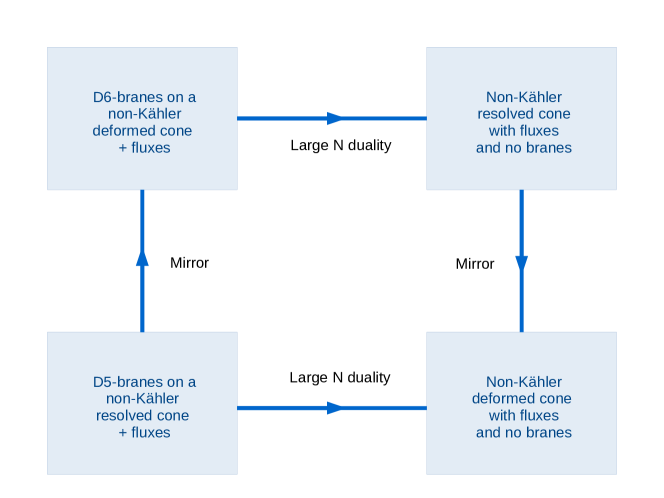
Figure 13: The web of dualities that connect various configurations in type IIB and type IIA theories. Here we will concentrate mostly on the lower left hand box that captures the physics of D5-branes wrapped on the two-cycle of a non-Kähler resolved conifold.

There appears to be some mismatch between the locations of four-dimensional gauge theory and the three-dimensional Chern-Simons theory. The four-dimensional ${\cal N}=1$ gauge theory is defined along the space-time directions ($x_{0},x_{1},x_{2},x_{3}$). Although this is slightly different from our earlier case, where the four-dimensional gauge theory was located along ($x_{0},x_{1},x_{2},\psi$) directions, it is nevertheless consistent with both the brane configurations in Table 2 as well as the configuration after a duality to a non-Kähler resolved conifold with wrapped D5-branes. However what is different now is the location of the Chern-Simons theory. Previously the Chern-Simons theory was localized to the boundary ${\bf W}$ of the four-dimensional space. For the present case the Chern-Simons theory is most succinctly described on the three-cycle ${\bf S}_{(2)}^{3}$ of a deformed conifold got by taking the mirror of the resolved conifold picture with wrapped D5-branes.

This apparent mismatch of the location of the Chern-Simons theory is not just a relocalization of the topological theory, but lies at the heart of the problem. To see this, first note that the partition function of the Chern-Simons theory on ${\bf S}_{(2)}^{3}$ in the large $N$ limit, takes the following form [7]:

$$Z\left[{\bf S}_{(2)}^{3}\right]={\rm exp}\left[-\sum_{g=0}^{\infty}\lambda^{2g-2}F_{g}(t)\right],$$ (393)

where $\lambda$ is the string coupling and $t=i\lambda N$ is the Kähler modulus of the blown-up ${\bf S}^{2}$ of a resolved conifold. This resolved conifold is not the same one studied in (4.1) above. Rather it is the one that appears to the top right of Fig 13. The factor $g$ in (393) is the genus $g$ of Riemann surfaces that parametrize the moduli space ${\cal M}_{g}$ with Euler characteristics $\chi_{g}$. Together they can be used to define $F_{g}(t)$, for $g\geq 2$, appearing in (393) as (see [42], and [8] for details):

$$F_{g}(t)~{}\equiv~{}\int_{{\cal M}_{g}}c_{g-1}^{3}-{\chi_{g}\over(2g-3)!}\sum_{n=1}^{\infty}n^{2g-3}e^{-nt},$$ (394)

where the first term denotes the Chern class of the Hodge bundle over the moduli space ${\cal M}_{g}$, derived in [42]. As noted in [7], (394) is very suggestive of a $g$-loop topological string amplitude.

Secondly, there are two different ways we can study knots here as mentioned above. The first is with intersecting D4-branes where a set of $N$ D4-branes wrap ${\bf S}_{(2)}^{3}\times{\bf R}^{2}$ and another set of $M$ D4-branes intersect the first set on the knot ${\bf K}$ and are stretched along the remaining directions ${\bf R}^{2}\times{\bf D}^{2}$, where ${\bf D}^{2}$ is a two-dimensional subspace in $T^{\ast}{\bf S}_{(2)}^{3}$. The second is with $N$ D6-branes wrapping ${\bf R}^{4}\times{\bf S}_{(2)}^{3}$. Once we go to Euclidean space, the knots appearing on ${\bf S}_{(2)}^{3}$ may be constructed using D2- or D4-branes intersecting the D6-branes on ${\bf K}$. Clearly it is the second case that is more relevant to us because the brane configuration given in Table 2 take us directly to this set-up via a series of T and SYZ [44, 45] dualities as shown in fig 13, at least in the absence of knots. Knots can then be inserted in the type IIA picture by surface operators.

It turns out, for the case that we are most interested in, the topological string amplitude $F_{g,h}$ with $g=0$ and $h=1$ computes the superpotential terms for the ${\cal N}=1$ theories in four-dimensions. The superpotential terms are in general harder to compute in type IIA language, but become easier in the mirror type IIB language. The mirror is of course our configuration of D5-branes wrapped on the two-cycle of a non-Kähler resolved conifold, bringing us back to the analysis performed in section 4.1.

The above discussion should hopefully suggest the usefulness of the type IIB analysis. However we haven’t yet reconconciled with all the steps of our earlier analysis performed in section 3. For example, if we want to localize the knots to the three-cycle ${\bf S}_{(2)}^{3}$ of the deformed conifold, what is the usefulness of the boundary ${\bf W}$ used earlier?

The answer can be given in a few steps. First, let us go back to the type IIB D5-$\overline{\rm D5}$ branes wrapped on the two-cycle of our Taub-NUT space discussed in section 3.1. We can move the $\overline{\rm D5}$-branes away on the Coulomb branch so that we are left with only D5-branes wrapped on the two-cycle of the Taub-NUT space. The geometry is discussed in (14) before. To go from this geometry to the one studied above in (4.1), we will assume that our Taub-NUT space is fibered over a ${\bf P}^{1}$, in other words, a resolved conifold geometry may be viewed as a Taub-NUT space fibered over a ${\bf P}^{1}$. The precise relationship between the two geometries is studied in section 3.1 of [46] (see equations (3.10) to (3.13) in [46]). The only difference here is now that the two-cycle, on which we have our wrapped D5-branes, should be along ($\theta_{1},\phi_{1}$). This is of course just a renaming of coordinates from section 3. The fibration breaks the four-dimensional supersymmetry down to ${\cal N}=1$, but for the time being we will not be too concerned with the supersymmetry. The above manipulation tells us how we can channel our earlier calculations for the new set-up. Locally, at every point on the base ${\bf P}^{1}$, parametrized by ($\theta_{2},\phi_{2}$), we have D-branes wrapped on the two-cycle of a Taub-NUT space.

Secondly, we go to Euclidean space and assume that the spacetime directions with Minkowskian coordinates ($x_{0},x_{1},x_{2}$) are now on an Euclidean ${\bf S}_{(1)}^{3}$. Thus the four-dimensional space ${\bf V}={\bf W}\times{\bf R}^{+}$ previously, now becomes ${\bf S}_{(1)}^{3}$ that represents ${\bf W}$ and the half coordinate $x_{3}$ that parametrizes ${\bf R}^{+}$. Further, the four-dimensional theory that we have on ${\bf S}_{(1)}^{3}\times{\bf R}^{+}$ can also be got from the mirror construction of D6-branes wrapped on three-cycle of a non-Kähler deformed conifold. Since they are connected by SYZ transformations [44, 45], the theories on ${\bf V}$, and therefore also on ${\bf W}$, are identical.

The above discussions suggest that we can perform similar computations in type IIB theory as in section 3, but now appropriately modified to incorporate D5-branes wrapped on two-cycle of a non-Kähler resolved conifold. This is easier than the mirror computations with D6-branes, and one may now insert the knots using surface operators on ${\bf S}^{3}$. Since the mirror picture is identical, we can view the theory on ${\bf S}_{(1)}^{3}$, got from our IIB computations, to be exactly the same in the type IIA side.

In the type IIA side, as shown on fig 13, the D6-branes are wrapped on the three-cycle ${\bf S}_{(2)}^{3}$ of a non-Kähler deformed conifold. In fact the world-volume of the D6-branes is oriented along ${\cal M}_{7}$ where:

$${\cal M}_{7}~{}\equiv~{}{\bf S}_{(1)}^{3}~{}\times~{}{\bf S}_{(2)}^{3}~{}\times~{}{\bf R}^{+},$$ (395)

and the physics on the first three-cycle ${\bf S}_{(1)}^{3}$ is directly imported from our type IIB analysis. Since the deformed conifold is non-compact, Gauss’ law is not violated and the wrapped D6-branes continue to be a valid supergravity solution there. We can now perform the following flop operation:

$${\bf S}_{(1)}^{3}~{}\leftrightarrow~{}{\bf S}_{(2)}^{3},$$ (396)

transferring all the physics on ${\bf S}_{(1)}^{3}$ to the three-cycle of the non-Kähler deformed conifold. This is exactly the D6-brane realization of the Ooguri-Vafa [8] model! Our construction differs from the intersecting D4-branes’ realization of the Ooguri-Vafa model in [11, 43].

The above discussions suggest the power of the IIB analysis: we can continue working on the type IIB side, albeit with a different background, and perform similar manipulations as in section 3. Of course subtleties appear because of the underlying supersymmetry, twisting etc, but presumably none too unsurmountable. Remarkably, once we have the full IIB analysis at hand, we can transfer the physics to the type IIA side by a mirror transformation followed by a flop operation (396) giving us the full realization of the Ooguri-Vafa [8] model. Therefore in the following we will elaborate on the type IIB side, by analyzing the background with and without dipole deformation and then discuss how to extract the four-dimensional physics similar to what we did in section 3. Most of the other details regarding the subtleties coming from reduced supersymmetry, twisting and the exact boundary theory on ${\bf S}_{(1)}^{3}$; including the type IIA mirror and the flop operation (396) will only be briefly touched upon here, and detailed elaborations will be relegated to the sequel.

4.2 Five branes on a resolved conifold: Exact results

Let us now consider specific choices of the warp factors $F_{i}(r)$ that would not only solve the EOMs but also preserve supersymmetry. One solution that was briefly mentioned in [40] and studied in some details in [46] is:

$$F_{1}={e^{-\phi}\over 2F},~{}~{}~{}~{}~{}F_{2}={r^{2}e^{-\phi}F\over 2},~{}~{}~{}~{}~{}F_{3}={r^{2}e^{-\phi}\over 4}+a^{2}(r),~{}~{}~{}~{}~{}F_{4}={r^{2}e^{-\phi}\over 4},$$ (397)

where $a^{2}\equiv a_{0}^{2}+a_{1}(r)$ and $a_{0}^{2}$ is the resolution parameter, $F(r)$ is some function of $r$ whose value will determined soon and $\phi$, as usual, is related to the type IIB dilaton. The function $F(r)$ has to be related to the dilaton $\phi(r)$ because any arbitrary choice of $F$ and $\phi$ will break supersymmetry. We will determine the equation relating $F$ and $\phi$ using torsion classes [49, 50, 51, 52]. In the process we will also argue for supersymmetry.

4.2.1 Analysis of the background fluxes

Before we go about determing the functional form for $r$, let us work out the three-form fluxes from (390). Plugging (397) into (390), they are given by:

$${\cal H}_{3}={1\over 4}{\rm sinh}~{}\beta~{}e^{-\phi}~{}r^{2}\left[\left(\phi_{r}-{8a\over r^{2}}e^{\phi}a_{r}\right)e_{r}\wedge e_{\theta_{1}}\wedge e_{\phi_{1}}+\phi_{r}~{}e_{r}\wedge e_{\theta_{2}}\wedge e_{\phi_{2}}\right]$$

$${\cal F}_{3}=-{1\over 4}{\rm cosh}~{}\beta~{}e^{\phi}~{}r^{3}F(r)\left[\left(1+{4a^{2}\over r^{2}}e^{\phi}\right)\phi_{r}~{}e_{\psi}\wedge e_{\theta_{1}}\wedge e_{\phi_{1}}+\left({r^{2}\phi_{r}-8aa_{r}e^{\phi}\over r^{2}+4a^{2}e^{\phi}}\right)e_{\psi}\wedge e_{\theta_{2}}\wedge e_{\phi_{2}}\right].$$

Looking carefully at the three-forms we see that ${\cal H}_{3}$ is closed but ${\cal F}_{3}$ is not. This is good because non-closure of ${\cal F}_{3}$ is related to the wrapped five-brane sources. Recall that the five-branes are wrapped on the two-cycle ($\theta_{1},\phi_{1}$) and stretched along the space-time directions $x_{0,1,2,3}$, which will be later converted to Euclidean ${\bf S}^{3}_{(1)}\times{\bf R}^{+}$. This means the source equation should have delta function like singularity along the orthogonal directions of the brane, namely the ($\theta_{2},\phi_{2},\psi$) and the radial direction $r$. In the limit when both $a^{2}$ as well as $a_{r}$ are smaller than some chosen scale in the theory, ${\cal F}_{3}$ can be expressed in the following suggestive way:

$${\cal F}_{3} = -{1\over 4}~{}{\rm cosh}~{}\beta~{}e^{\phi}r^{3}F~{}\phi_{r}~{}e_{\psi}\wedge\left(e_{\theta_{1}}\wedge e_{\phi_{1}}-e_{\theta_{2}}\wedge e_{\phi_{2}}\right)$$

$$-{\rm cosh}~{}\beta~{}e^{2\phi}rF~{}e_{\psi}\wedge\left[{\hat{a}}^{2}~{}e_{\theta_{1}}\wedge e_{\phi_{1}}-{\hat{a}}^{2}~{}e_{\theta_{2}}\wedge e_{\phi_{2}}-\left(2aa_{r}-{1\over 2}e^{-\phi}r^{2}\phi_{r}\right)e_{\theta_{2}}\wedge e_{\phi_{2}}\right]$$

where the implications of the relative sign between the vielbein products will become clear soon. We have also defined:

$${\hat{a}}^{2}=a^{2}\phi_{r}.$$ (400)

As mentioned earlier, ${\cal F}_{3}$ is not closed, and therefore $d{\cal F}_{3}$ should be related to localized or delocalized sources along the ($\theta_{2},\phi_{2}$) and ($r,\psi$) directions. Using the fact that the three-form:

$$\eta_{3}\equiv e_{\psi}\wedge\left(e_{\theta_{1}}\wedge e_{\phi_{1}}-e_{\theta_{2}}\wedge e_{\phi_{2}}\right)$$ (401)

is closed we can find some relations between the three unknown functions $F(r),\phi(r)$ and $a(r)$ that appear in (4.2.1). All we need is to express the dilaton $\phi(r)$ and the resolution parameter $a(r)$ in terms of the function $F(r)$ that appears in our ansatze (397). One simple relation between the three variables is given by:

$${de^{\phi}\over dr}\left({1\over 4}+{e^{\phi}~{}a^{2}\over r^{2}}\right)={c_{0}\over r^{3}F},$$ (402)

where $c_{0}$ is a constant whose value could be determined from the boundary condition. Note that this is an additional constraint compared to [46]. Pluging in (402) in (4.2.1), we get:

$${{\cal F}_{3}\over{\rm cosh}~{}\beta}=-c_{0}~{}\eta_{3}+\left(2aa_{r}-{1\over 2}e^{-\phi}r^{2}\phi_{r}\right)e^{2\phi}rF~{}e_{\psi}\wedge e_{\theta_{2}}\wedge e_{\phi_{2}}.$$ (403)

The source equation is now easy to determine from (403). It is clear that the first term does not contribute, and the contribution therefore solely comes from the second term of (403):

$$d{\cal F}_{3}=G_{r}(r)~{}e_{r}\wedge e_{\psi}\wedge e_{\theta_{2}}\wedge e_{\phi_{2}}-G(r)~{}e_{\theta_{1}}\wedge e_{\phi_{1}}\wedge e_{\theta_{2}}\wedge e_{\phi_{2}}$$ (404)

with $G(r)$ defined as:

$$G(r)=\left(2aa_{r}-{1\over 2}e^{-\phi}r^{2}\phi_{r}\right)e^{2\phi}rF~{}{\rm cosh}~{}\beta.$$ (405)

Looking at (404) we see that we have two terms. The first term of (404) captures the Gauss’ charge along the orthogonal directions of the wrapped D5-branes i.e the ($r,\psi,\theta_{2},\phi_{2}$) directions. The second term, that is proportional to the volume of the four-cycle, captures the Gauss’ charge along the ($\theta_{2},\phi_{2}$) directions. In fact this term tells us that even if $G(r)$ is a constant, the D5-branes’ charge would be calculable.

We see that there are two constraint equations, (402) and (404), for three functions $F(r),e^{\phi}$ and $a(r)$. The third equation will be determined soon when we will demand supersymmety in the system. We could also go for more generic solution to the system. Constraint on D5-brane charges impose the following relation between the four warp factors $F_{i}(r)$ and the dilaton $e^{\phi}$:

$${dF_{4}\over dr}=\sqrt{F_{1}F_{2}}\left(1-{e^{-2\phi}F_{4}\over F_{2}F_{3}}\right).$$ (406)

One may compare this with the recently found constraint relations in [40]. Since we are not imposing integrable complex structures, we don’t have additional constraint equations as in [40]. Note also that an equation like (406) is not required in the heterotic theory as the anomalous Bianchi identity is enough [46]. Thus plugging in (406) in (390) we get:

$${{\cal F}_{3}\over{\rm cosh}~{}\beta}=-\eta_{3}-\left[1+e^{2\phi}{F_{4}\over F_{3}}\sqrt{F_{2}\over F_{1}}\left(\sqrt{F_{1}F_{2}}-F_{3r}\right)\right]~{}e_{\psi}\wedge e_{\theta_{2}}\wedge e_{\phi_{2}}.$$ (407)

The second constraint would come from (407) if we demand charge quantization. Of course if the D5-brane charges are delocalized there is no strong constraint being imposed by (407). However demanding supersymmetry does introduce new constraint on the warp factors. In the following section we will use the powerful machinery of the torsion classes ${\cal W}_{i}$ [49] to analyze this.

4.2.2 Finding the warp factors using torsion classes

To study the constraint on the warp factors one may use the technique of the torsion classes [49]. For us the relevant torsion classes are the ${\cal W}_{4}$ and ${\cal W}_{5}$ classes, defined as:

$$\mathcal{W}_{4}={F_{3r}-\sqrt{F_{1}F_{2}}\over 4F_{3}}+{F_{4r}-\sqrt{F_{1}F_{2}}\over 4F_{4}}+\phi_{r},$$

$${\rm Re}~{}\mathcal{W}_{5}={F_{3r}\over 12F_{3}}+{F_{4r}\over 12F_{4}}+{F_{2r}-2\sqrt{F_{1}F_{2}}\over 12F_{2}}+{\phi_{r}\over 2},$$ (408)

where one may look at the detailed derivations from [46, 40] or some of the earlier papers in the series namely [47, 48] etc. Plugging in the warp factor choice (397), it is easy to see that:

$${\cal W}_{4}={\phi_{r}\over 2}+{\cal O}(a^{2})$$

$${\cal W}_{5}\equiv{\rm Re}~{}{\cal W}_{5}={1\over 12}\left({6\over r}+3\phi_{r}+{F_{r}\over F}-{2\over rF}\right).$$ (409)

Depending on how to define our dilaton,

$${\rm Re}~{}{\cal W}_{5}=\pm\phi_{r}+{\cal O}(a^{2}),$$ (410)

such that the supersymmetry condition will take the following well-known form in terms of the torsion classes [50, 51, 52]:

$$2{\cal W}_{4}\pm{\rm Re}~{}{\cal W}_{5}=0.$$ (411)

For us we will choose the minus sign in (410) such that (411) will appear with a relative plus sign. This gives the following equation for the variables $F(r)$ and $e^{\phi}$ upto ${\cal O}(a^{2})$:

$$r{d\phi\over dr}+{r\over 15F}{dF\over dr}-{2\over 15F}+{2\over 5}+{\cal O}(a^{2})=0.$$ (412)

The above is the simplified version where the dependence of the resolution parameter is not shown. If we insert $a^{2}$, the EOM becomes more involved and takes the following form:

$$\left(15+{88a^{2}e^{\phi}\over r^{2}}\right){d\phi\over dr}+{56e^{\phi}a\over r^{2}}{da\over dr}+\left({4\over r}+{1\over F}{dF\over dr}-{2\over rF}\right)\left(1+{4a^{2}e^{\phi}\over r^{2}}\right)+{2\over r}=0,$$

and reduces to (412) in the limit where $a^{2}$ as well as $da/dr$ are small. In this limit we can combine (402) and (412) to eliminate $F(r)$ and express everything in terms of the following dilaton equation:

$$r{d^{2}Z\over dr^{2}}-3{dZ\over dr}+r\left({r^{2}\over 2c_{0}}-{15\over Z}\right)\left({dZ\over dr}\right)^{2}=0$$ (414)

where $Z=e^{\phi}$ and $c_{0}$ is a constant appearing in (402). To solve the above equation let us take the following ansatze for $Z$:

$$Z(r)~{}=~{}{\alpha(r)\over r^{2}},$$ (415)

with $\alpha(r)$ a positive definite function for all $r$. Plugging (415) in (414), we see that $\alpha(r)$ satisfies the following second-order differential equation:

$$c_{0}{d^{2}\alpha\over dr^{2}}+\left({53c_{0}-2\alpha\over r}\right){d\alpha\over dr}+\left({1\over 2}-{15c_{0}\over\alpha}\right)\left({d\alpha\over dr}\right)^{2}+{2\alpha(\alpha-24c_{0})\over r^{2}}=0.$$ (416)

One simple solution for the system is given by a constant $\alpha$, i.e:

$$\alpha~{}=~{}24c_{0}.$$ (417)

Other solutions to (416) could be entertained but we will not do so here. Plugging (417) in (415) and (402), and using the definition of $Z$, we find that:

$$e^{\phi}={24c_{0}\over r^{2}},~{}~{}~{}~{}~{}~{}~{}~{}F=-{1\over 12}.$$ (418)

The careful reader will be alarmed by seeing the negative value for $F$ because $F$ goes into the definition for the warp-factors in (397). However if we look at (397) carefully, we see that $F$ appears in the definitions of $F_{1}$ and $F_{2}$ but not in the definitions of $F_{3}$ and $F_{4}$. This is good because ($F_{1},F_{2}$) appear in the three-form fluxes ${\cal H}_{3}$ and ${\cal F}_{3}$ only in the combinations $F_{1}F_{2}$ and $F_{2}/F_{1}$. Thus we can change the sign of ($F_{1},F_{2}$) simultaneously without changing the fluxes or the constraint equation (402)! The consequence of this invariance is simply the following changes to the definition of the warp factors:

$$F_{1}~{}\to~{}|F_{1}|,~{}~{}~{}~{}~{}~{}~{}F_{2}~{}\to~{}|F_{2}|,$$ (419)

without changing $F_{3}$ and $F_{4}$. This means, after the dust settles, the internal six-dimensional manifold in type IIB theory will be given by the following metric:

$$ds_{6}^{2} = {r^{2}\over 4c_{0}}\Big{[}dr^{2}+{r^{2}\over 144}\left(d\psi+{\rm cos}~{}\theta_{1}~{}d\phi_{1}+{\rm cos}~{}\theta_{2}~{}d\phi_{2}\right)^{2}$$ (420)

$$+\left({r^{2}\over 24}+{\cal O}(a^{2})\right)(d\theta_{1}^{2}+{\rm sin}^{2}\theta_{1}~{}d\phi_{1}^{2})+{r^{2}\over 24}(d\theta_{2}^{2}+{\rm sin}^{2}\theta_{2}~{}d\phi_{2}^{2})\Big{]}.$$

The above metric is a non-Kähler metric on the resolved conifold, and can be compared to the recently studied examples in [40]. If we change our initial ansatze (397), we can allow for a different non-Kähler metric on the resolved conifold. There is of course an infinite class of possible non-Kähler metric that we can allow for a given complex structure and satisfying the constraint equation (406) and the supersymmetry condition (411) with a relative plus sign between the ${\cal W}_{4}$ and ${\cal W}_{5}$ torsion classes. The generic solution for the metric and the three-form fluxes with these constraints will then be (390). For the specific choice (420) of the internal metric, the three-form fluxes are given by:

$${\cal F}_{3}=+c_{0}~{}{\rm cosh}~{}\beta~{}e_{\psi}\wedge\left(e_{\theta_{1}}\wedge e_{\phi_{1}}+e_{\theta_{2}}\wedge e_{\phi_{2}}\right)$$

$${\cal H}_{3}=-{r^{3}\over 48c_{0}}~{}{\rm sinh}~{}\beta~{}e_{r}\wedge\left(e_{\theta_{1}}\wedge e_{\phi_{1}}+e_{\theta_{2}}\wedge e_{\phi_{2}}\right),$$ (421)

with the five-form flux derivable from (4.2.2) and (390). The IIB dilaton, on the other hand, is $e^{\phi_{B}}=e^{-\phi}$ and so for

$$r~{}\geq~{}\sqrt{24c_{0}},$$ (422)

classical supergravity solution will not capture the full dynamics and one has to go to it S-dual, or weakly coupled version of the theory. Combining the two patches, one should be able to study the sugra limit of the theory.

On the other hand if dilaton is slowly varying from its weak coupling value then one may express (4.2.2) as:

$${da^{2}\over dr}+{1\over 28}\left(4r+{r^{2}\over F}{dF\over dr}-{2r\over F}\right)\left(e^{-\phi}+{4a^{2}\over r^{2}}\right)+{re^{-\phi}\over 14}=0.$$ (423)

To solve (423), let us assume that the dilaton is given by the following expression in terms of a slowly varying function $f(r)$:

$$e^{\phi}~{}=~{}e^{\phi_{0}}+f(r),$$ (424)

where the constant factor is the weak coupling limit. To proceed, let us define two functions $H(x)$ and $G(x)$ using the function $F(x)$ appearing in (423), in the following way:

$$G(x)={1\over 7}\left({4\over x}-{2\over xF(x)}+{F^{\prime}(x)\over F(x)}\right),~{}~{}~{}~{}~{}H(x)=xe^{-\phi_{0}}\left({xG(x)\over 4}+{1\over 14}\right),$$ (425)

where the prime is defined as the derivative of $x$. Using (424) and (425), we can solve for the resolution parameter $a^{2}$ in terms of the functions $G(x)$ and $H(x)$ as:

$$a^{2}(r)=-\int_{0}^{r}dy~{}H(y)~{}{\rm exp}\left(\int_{r}^{y}dx~{}G(x)\right)+{\cal O}(f),$$ (426)

where the overall negative sign shouldn’t be a concern because the functional form for $F(x)$ will be chosen so that $a^{2}$ remains positive definite.

4.3 A four-fold from the $G_{2}$ structure manifold in M-theory

In the previous section we discussed possible ways to construct the metric of D5-branes wrapped on two-cycle of a non-Kähler resolved conifold. We discussed a class of these solutions satisfying the charge constraint (406) and the supersymmetry constraint (411). The M-theory uplift of these solutions can be done by first T-dualizing along $\psi$ direction to allow for D6-branes in type IIA theory oriented along ($\theta_{1},\phi_{1},\psi$) and spanning the space-time directions $x_{0,1,2,3}$. We can then lift this configuration to M-theory on a $G_{2}$ structure manifold. The way we constructed our scenario, T-duality of the IIB configuration will lead to D6-branes and not D4-branes as in [21, 19]. At low energies, and as discussed around (8), we do get the D4-branes configuration (see also [40]). Furthermore, we will start by studying a single D6-brane and insert the dipole deformation of the T-dual wrapped D5-brane. Later on we will generalize this to multiple D6-branes.

4.3.1 First look at the $G_{2}$ structure manifold

The D6-brane configuration, without dipole deformation of the T-dual wrapped D5-brane on non-Kähler resolved conifold, is given by the following metric structure on an internal six-dimensional space:

$$ds^{2} = {1\over\sqrt{h}}~{}ds^{2}_{012}+{1\over\sqrt{h}}\left(dx_{3}^{2}+{1\over F_{2}}~{}d\psi^{2}\right)$$ (427)

$$+ \sqrt{h}\left[F_{1}dr^{2}+F_{3}(d\theta_{1}^{2}+{\rm sin}^{2}\theta_{1}~{}d\phi_{1}^{2})+F_{4}(d\theta_{2}^{2}+{\rm sin}^{2}\theta_{1}~{}d\phi_{2}^{2})\right],$$

where we have separated the compact directions ($x_{3},\psi$) in anticipation of the dipole deformations along those directions in the type IIB side. The type IIA dilaton $e^{\phi_{A}}$ and the warp factor $h$ are defined in the following way:

$$e^{\phi_{A}}\equiv e^{-\phi}F_{2}^{-1/2}h^{-1/4},~{}~{}~{}~{}h\equiv e^{2\phi}~{}{\rm cosh}^{2}\beta-{\rm sinh}^{2}\beta,$$ (428)

such that when $\beta=0$ we get back the standard picture. Combining the IIA metric (427) with the dilaton (428) we can easily get the M-theory manifold as:

$$ds^{2}_{11}={e^{2\phi/3}F_{2}^{1/3}\over h^{1/3}}~{}ds^{2}_{012}+ds^{2}_{8}$$ (429)

where $ds^{2}_{8}$ is a eight-dimensional manifold that, in the absence of the dipole deformation in the type IIB side, is simply a $S^{1}$ fibration over a $G_{2}$ structure seven-manifold expressed as:

$$ds^{2}_{8} = {e^{2\phi/3}F_{2}^{1/3}\over h^{1/3}}\left(dx^{2}_{3}+{1\over F_{2}}d\psi^{2}\right)+{1\over e^{4\phi/3}F_{2}^{2/3}h^{1/3}}(dx_{11}+{\bf A}_{1\mu}dx^{\mu})^{2}$$

$$+ e^{2\phi/3}F_{2}^{1/3}h^{2/3}\left[F_{1}dr^{2}+F_{3}(d\theta_{1}^{2}+{\rm sin}^{2}\theta_{1}~{}d\phi_{1}^{2})+F_{4}(d\theta_{2}^{2}+{\rm sin}^{2}\theta_{2}~{}d\phi_{2}^{2})\right].$$

The ${\bf A}_{1}$ appearing above is the type IIA gauge field whose value will be determined soon. As discussed in details in [40], the $G_{2}$ structure seven-manifold in-turn is a four-dimensional warped Taub-NUT manifold $ds^{2}_{\rm TN}$ fibered over a three-dimensional base $ds_{3}^{2}$ parametrized by ($\theta_{1},\phi_{1},\psi$):

$$ds^{2}_{7} = ds^{2}_{3}+ds^{2}_{\rm TN}$$ (431)

$$= G_{2}\left(d\theta_{1}^{2}+{\rm sin}^{2}\theta_{1}~{}d\phi_{1}^{2}+{G_{1}\over G_{2}F_{2}}d\psi^{2}\right)$$

$$+ G_{3}dr^{2}+G_{4}\left(d\theta_{2}^{2}+{G_{5}\over G_{4}}d\phi_{2}^{2}\right)+G_{6}\left(dx_{11}+{\bf A}_{1\mu}dx^{\mu}\right)^{2},$$

where $G_{i}$ are the warp factors that can be read up from (4.3.1) or from [40] and the third line of (431) is the metric of the warped Taub-NUT space.

4.3.2 Dipole deformation and the M-theory uplift

It is now time to see what effect would the type IIB dipole deformation have on our M-theory manifold. Dipole deformation of four-dimensional Yang-Mills theory was first introduced from gauge theory side in [24] and from type IIB gravity dual in [25, 26]. Elaborate study was performed in [53, 54]. Essentially the simplest dipole deformation amounts to switching on a NS B-field with one component along the brane and the other component orthogonal to the brane. Generalization of this picture exists, but we will not discuss this here. The B-field for our case will have component $B_{3\psi}$ as we mentioned before, which of course has the required property in the presence of a D5-brane along ($x_{0,1,2,3},\theta_{1},\phi_{1}$). However as before this B-field cannot be a constant otherwise it will be gauged away. Thus again we expect a field strength of the form $dB$, which in turn will then back-react on our original type IIB background (390) and change the metric to the following:

$$ds^{2} = {1\over\sqrt{h}}\left(-dt^{2}+dx_{1}^{2}+dx_{2}^{2}+{dx_{3}^{2}\over{\rm cos}^{2}~{}\theta+F_{2}~{}{\rm sin}^{2}~{}\theta}\right)$$

$$+ \sqrt{h}\left[F_{1}dr^{2}+{F_{2}({d\psi\over{\rm cos}~{}\theta}+{\rm cos}~{}\theta_{1}~{}d\phi_{1}+{\rm cos}~{}\theta_{2}~{}d\phi_{2})^{2}\over 1+F_{2}~{}{\rm tan}^{2}~{}\theta}+\sum_{i=1}^{2}F_{2+i}\left(d\theta_{i}^{2}+{\rm sin}^{2}~{}\theta_{i}~{}d\phi_{i}^{2}\right)\right],$$

where $\theta$ is the dipole deformation parameter. The three-form fluxes also change from their values in (390) to the following:

$${\cal F}_{3} = -e^{2\phi}~{}{\rm cosh}~{}\beta\sqrt{F_{2}\over F_{1}}\left(g_{1}~{}{\widetilde{e}_{\psi}}\wedge e_{\theta_{1}}\wedge e_{\phi_{1}}+g_{2}~{}{\widetilde{e}_{\psi}}\wedge e_{\theta_{2}}\wedge e_{\phi_{2}}\right)$$

$${\cal H}_{3} = {\rm sinh}~{}\beta\left[\left(\sqrt{F_{1}F_{2}}-F_{3r}\right)e_{r}\wedge e_{\theta_{1}}\wedge e_{\phi_{1}}+\left(\sqrt{F_{1}F_{2}}-F_{4r}\right)e_{r}\wedge e_{\theta_{2}}\wedge e_{\phi_{2}}\right]$$

$$+{F_{2r}~{}{\rm sin}~{}2\theta\over 2\left({\rm cos}^{2}~{}\theta+F_{2}~{}{\rm sin}^{2}~{}\theta\right)^{2}}~{}e_{r}\wedge{\widetilde{e}_{\psi}}\wedge e_{3}+{F_{2}~{}{\rm sin}~{}\theta\over{\rm cos}^{2}~{}\theta+F_{2}~{}{\rm sin}^{2}~{}\theta}\sum_{i=1}^{2}e_{\phi_{i}}\wedge e_{\theta_{i}}\wedge e_{3}$$

where as before we note that the dipole deformation has appeared as an additional term in the definition of the three-form flux ${\cal H}_{3}$, and helped to break the Lorentz invariance between $x_{0,1,2}$ and $x_{3}$ directions. The type IIB dilaton $e^{\phi_{B}}$ and ${\widetilde{e}_{\psi}}$ are defined in the following way:

$$e^{\phi_{B}}={e^{-\phi}\over\sqrt{{\rm cos}^{2}~{}\theta+F_{2}~{}{\rm sin}^{2}~{}\theta}},~{}~{}~{}~{}{\widetilde{e}_{\psi}}=d\psi+{\rm cos}~{}\theta_{1}~{}{\rm cos}~{}\theta~{}d\phi_{1}+{\rm cos}~{}\theta_{2}~{}{\rm cos}~{}\theta~{}d\phi_{2}.$$

The M-theory uplift of the dipole-deformed type IIB set-up is now easy to perform once we get the type IIA configuration. The type IIA dilaton does not change from its value (428), and the only change in the metric (427) is:

$${1\over\sqrt{h}}\left(dx_{3}^{2}+{1\over F_{2}}~{}d\psi^{2}\right)~{}~{}\to~{}~{}{1\over\sqrt{h}}\left[{dx_{3}^{2}\over{\rm cos}^{2}~{}\theta}+2{\rm tan}~{}\theta~{}dx_{3}d\psi+\left({\rm sin}^{2}~{}\theta+{{\rm cos}^{2}~{}\theta\over F_{2}}\right)d\psi^{2}\right],$$

which means the M-theory metric retain its form (429) except the metric of the eight manifold changes slightly from (4.3.1) to the following metric:

$$ds^{2}_{8} = {e^{2\phi/3}F_{2}^{1/3}\over h^{1/3}{\rm cos}^{2}~{}\theta}~{}{\bf|}dx_{3}+\tau_{1}~{}d\psi{\bf|}^{2}+{1\over e^{4\phi/3}F_{2}^{2/3}h^{1/3}}(dx_{11}+{\bf A}_{1\mu}dx^{\mu})^{2}$$

$$+ e^{2\phi/3}F_{2}^{1/3}h^{2/3}\left[F_{1}dr^{2}+F_{3}(d\theta_{1}^{2}+{\rm sin}^{2}\theta_{1}~{}d\phi_{1}^{2})+F_{4}(d\theta_{2}^{2}+{\rm sin}^{2}\theta_{2}~{}d\phi_{2}^{2})\right],$$

where the complex structure $\tau_{1}$ of the ($x_{3},\psi$) torus is given by:

$$\tau_{1}~{}=~{}{\rm sin}~{}\theta~{}{\rm cos}~{}\theta+{i{\rm cos}^{2}~{}\theta\over\sqrt{F_{2}}}.$$ (437)

Note that the warped Taub-NUT space doesn’t change from what we had earlier in (4.3.1) without dipole deformation. The gauge field ${\bf A}_{1}$ in the Taub-NUT fibration structure also doesn’t change, and is given by the following field-strength:

$${{\cal F}_{2}\over{\rm cosh}~{}\beta} = -e_{\theta_{1}}\wedge e_{\phi_{1}}-e^{2\phi}\sqrt{F_{2}\over F_{1}}\cdot{F_{4}\over F_{3}}\left(\sqrt{F_{1}F_{2}}-F_{3r}\right)~{}e_{\theta_{2}}\wedge e_{\phi_{2}}$$ (438)

$$= {d{\bf A}_{1}\over{\rm cosh}~{}\beta}+\left[1-e^{2\phi}\sqrt{F_{2}\over F_{1}}\cdot{F_{4}\over F_{3}}\left(\sqrt{F_{1}F_{2}}-F_{3r}\right)\right]~{}e_{\theta_{2}}\wedge e_{\phi_{2}},$$

using the constraint (406) and defining the gauge field ${\bf A}_{1}$ in the following way:

$${\bf A}_{1}={\rm cosh}~{}\beta\left({\rm cos}~{}\theta_{1}~{}d\phi_{1}+{\rm cos}~{}\theta_{2}~{}d\phi_{2}\right),$$ (439)

which would appear in the fibration (4.3.2). However expressing the gauge field as (439) does not introduce any additional constraint on the warp-factors in the metric (see discussion in [40]). The ${\cal G}_{4}$ flux in M-theory can now be expressed as:

$${{\cal G}_{4}\over{\rm sinh}~{}\beta} = \left(\sqrt{F_{1}F_{2}}-F_{3r}\right)e_{r}\wedge e_{\theta_{1}}\wedge e_{\phi_{1}}\wedge e_{11}+{\rm cosech}~{}\beta~{}d\psi\wedge e_{\theta_{1}}\wedge e_{\phi_{1}}\wedge\widetilde{e}_{11}$$

$$+ \left(\sqrt{F_{1}F_{2}}-F_{4r}\right)e_{r}\wedge e_{\theta_{2}}\wedge e_{\phi_{2}}\wedge e_{11}+{\rm cosech}~{}\beta~{}d\psi\wedge e_{\theta_{2}}\wedge e_{\phi_{2}}\wedge\widetilde{e}_{11},$$

where we see that the dipole deformation appears in an appropriate way in the ${\cal G}_{4}$ flux. In the absence of the type IIB dipole deformation the form of (4.3.2) is almost similar to what we had in [40] except the vielbeins $e_{11}$ and $\widetilde{e}_{11}$ are defined in a slightly different way as:

$$e_{11}=dx_{11}+{\rm cos}~{}\theta~{}{\rm cosh}~{}\beta({\rm cos}~{}\theta_{1}~{}d\phi_{1}+g_{o}~{}{\rm cos}~{}\theta_{2}~{}d\phi_{2})$$ (441)

$$\widetilde{e}_{11}=dx_{11}+{\rm cos}~{}\theta~{}{\rm cosh}~{}\beta(g_{o}~{}{\rm cos}~{}\theta_{1}~{}d\phi_{1}+{\rm cos}~{}\theta_{2}~{}d\phi_{2}),$$

using the following functional form for $g_{o}(r)$:

$$g_{o}(r)=e^{2\phi}\sqrt{F_{2}\over F_{1}}\cdot{F_{4}\over F_{3}}\left(\sqrt{F_{1}F_{2}}-F_{3r}\right).$$ (442)

4.3.3 Revisiting gauge theory from M-theory

We have by now developed all the machinery needed for determining the gauge field on the wrapped D5-branes from M-theory. If we take a single wrapped D5-brane on the non-Kähler resolved conifold, the M-theory manifold (4.3.2) will be a warped single-centered Taub-NUT space fibered over a four-dimensional base parametrized by ($x_{3},\psi,\theta_{1},\phi_{1}$) coordinates. The gauge-field in the type IIB side will appear as localized G-flux in M-theory, similar to what we had earlier in section 3.2.3 (see also the discussion in [40]). For the single centered Taub-NUT case in (4.3.2), at any given point on four-dimensional base, the localized G-flux can be expressed as:

$${\cal G}_{4}^{\rm loc}={\cal F}\wedge\omega,$$ (443)

where ${\cal F}$ is the world-volume gauge field that, in the language of the wrapped D6-brane, will be along four-dimensional spacetime parametrized by $x_{0,1,2,3}$ coordinates. This of course parallels the story we discussed in great details in section 3.2.4. There is also an option to define the gauge theory along the compact ($\psi,\theta_{1},\phi_{1}$) directions, or even along all compact and non-compact directions. Each of these possibilities will lead to interesting interpretations for the knot invariants once we extend this to the non-abelian case. We will however only concentrate on the gauge theory along the spacetime directions so that comparison with earlier sections like 3.2.4, 3.2.5 and 3.2.6 as well as with [11] may be made easily. In fact we will follow similar logic as in sections 3.2.4 and 3.2.5, namely, study the abelian theory and then proceed to discuss the non-abelian case (which is the large $N$ limit here).

The abelian case is succinctly represented by $\omega$ in (443), which is a normalizable harmonic two-form, expressed as $\omega=d\zeta$. The procedure is similar to what we had in (55), (3.2.3) and (3.2.3), so we will avoid the details. Once the dust settles, $\zeta$ is given by the following expression:

$$\zeta(r,\theta_{2}) = g_{0}~{}{\rm exp}\left[-\int^{r}dr~{}{e^{-\phi}\over F_{4}}\sqrt{F_{1}\over hF_{2}}\right]\left(d\Psi+{\rm cos}~{}\theta_{2}~{}d\phi_{2}\right)$$

$$= g_{0}~{}{\rm exp}\left[-\int_{0}^{r}{48~{}dx\over x\sqrt{576c_{0}^{2}~{}{\rm cosh}^{2}~{}\beta-x^{4}~{}{\rm sinh}^{2}~{}\beta}}\right]\left(d\Psi+{\rm cos}~{}\theta_{2}~{}d\phi_{2}\right),$$

where $d\Psi=dx_{11}/{\rm cosh}~{}\beta$ and the second line is from using the background (418) and (420). Note that the harmonic form tells us that for:

$$r~{}>~{}\sqrt{24c_{0}~{}{\rm coth}~{}\beta},$$ (445)

new description has to be devised as the harmonic form will become oscillatory. This bound should be compared to (422) where strong coupling sets in for the radius equals $\sqrt{24c_{0}}$.

The non-abelian enhancement now follows similar procedure as outlined in section 3.2.6. The M2-brane states wrap around the Taub-NUT singularities to enhance the gauge symmetry to $SU(N)$. This way we will have ${\cal N}=1$ supersymmetric $SU(N)$ Yang-Mills theory in four spacetime dimensions appearing from $N$ D5-branes wrapped on the two-cycle of a non-Kähler resolved conifold.

4.4 Comparing knots from branes and from gravity duals

In the previous sections we have developed most of the machinery needed to study the abelian and the non-abelian theories on the wrapped D5-branes on a resolved conifold from M-theory point of view. Our aim is to concentrate on the non-abelian case with two goals in mind: the first is to study the connection between the model of Witten [11] using five-branes and the model of Ooguri-Vafa [8] using geometric transition picture to study knots invariants and Khovanov homology. The second goal is to use our M-theory picture to actually compute some of these invariants and develop the picture in more generic direction. A discussion of the first goal, namely connecting the two models: [11] and [8], is presented in section 4.1.1 and in the following we will elaborate the story a bit more.

Our starting point, which is the configuration of $N$ D5-branes wrapped on a two-cycle of a non-Kähler resolved conifold, may look a bit different from the configuration that we used before in section 3, namely, a finite number of D5-branes wrapped on the two-cycles of a warped Taub-NUT space. Additionally, the supersymmetry is now no longer ${\cal N}=4$, but is the minimal ${\cal N}=1$. The latter tells us that we have no Coulomb branch, implying that the vector multiplet is devoid of any scalar fields. Thus the twisting that we performed in section 3.2.12 to determine the boundary theory cannot be done in a similar way now. Additionally, we see that there are apparently two realizations of the Ooguri-Vafa model in M-theory from the type IIB configuration.

Using one T-duality: This will lead to the D6-branes that we studied above. Subsequent lift to M-theory results in the localized G-flux that has two legs along the spacetime $x_{0,1,2,3}$ directions and two legs along the Taub-NUT directions leading to gauge fields in the spacetime directions. The other components of the gauge fields in the internal directions will appear as non-abelian scalars in the non-compact three-dimensions. Together they will generate the ${\cal N}=1$ non-abelian vector multiplet with scalar fields forming the chiral multiplets.

Using three T-dualities: Instead of making one T-duality to go to the D6-brane picture, we can make three T-dualities to go to the mirror picture [44, 45]. Here we will again get D6-branes but wrapped on the three-cycle of a non-Kähler deformed conifold. Lifting this to M-theory this will lead to another $G_{2}$ structure manifold which is yet again a warped Taub-NUT space fibered over a three-dimensional base [46]. The localized G-flux can now be used to compute the four-dimensional theory as before.

As explained in section 4.1.1, despite appearance, the physics in four spacetime dimensions for both cases are identical. This is not a surprise because T-dualities generally do not change the four-dimensional physics. Thus either of the two configurations $-$ D5-branes wrapped on two-cycle of a resolved conifold or D6-branes wrapped on three-cycle of a deformed conifold $-$ may be used to study the Ooguri-Vafa [8] model. However since the latter is technically harder, we have used the type IIB model to study the four-dimensional physics above. Additionally since a non-Kähler resolved cone may be expressed as a warped Taub-NUT fibered over a ${\bf P}^{1}$ base [46], locally at a given point on ${\bf P}^{1}$, the D5-branes can be thought of as wrapping the two-cycle of the Taub-NUT space. We now see some resemblance with [11] locally, although the global picture is different. Unfortunately we cannot extend the similarity too far because, in the Ooguri-Vafa case, the absence of the Coulomb branch will not allow us to make similar manipulations as we did in section 3.2.12.

Despite this, the gauge theory derivation from M-theory in the previous section helps us to at least get the topological piece in a way similar to what we had in (71) before. Let us concentrate on the second piece in (71), namely the topological term. For the present case, it is more instructive to Euclideanize everthing, as we hinted in section 4.1.1. Assuming this, we get:

$$\int_{\Sigma_{11}}{\cal C}_{3}\wedge{\cal G}_{4}\wedge{\cal G}_{4}={\widetilde{c}}_{2}\int_{\Sigma_{4}}{\cal F}\wedge{\cal F},$$ (446)

where both $\Sigma_{11}$ and $\Sigma_{4}$ are eleven and four-dimensional Euclidean spaces respectively, and the coupling constant ${\widetilde{c}}_{2}$ is defined as:

$${\widetilde{c}}_{2}\equiv\int_{\Sigma_{7}}\langle{\cal C}_{3}\rangle\wedge\omega\wedge\omega,$$ (447)

with $\omega=d\zeta$ as described in (4.3.3) above, $\Sigma_{7}$ is the $G_{2}$ structure manifold in M-theory and $\langle{\cal C}_{3}\rangle$ is the expectation value of the three-form potential $\left({\cal C}_{3}\right)_{r\psi\phi_{1}}$ which may be extracted from the four-form ${\cal G}_{4}$ in (4.3.2) using the vielbeins (441).

One of the key difference between ${\widetilde{c}}_{2}$ in (447) and $c_{2}$ in (72) is the orientations of $\langle{\cal C}_{3}\rangle$ appearing in both. Previously we needed three-form potential of the form $\left({\cal C}_{3}\right)_{3r\phi_{1}}$ (76) to determine $c_{2}$ in (72). Such a component was generated from the subtle flux arrangement on the two-cycle of the warped Taub-NUT space to stabilize the D5-${\overline{\rm D5}}$ pairs against tachyonic instabilities. Now we don’t have such instabilities, and the three-form potential does appear more naturally from (4.3.2).

Once we allow for the non-abelian extension, the coefficient of the topological term ${\widetilde{c}}_{2}$ will remain the same as (447) with a $SU(N)$ trace inserted in the action (447), similar to what we had in section 3.2.6. The boundary theory may now be derived in a much simpler way that what we had in section 3.2.12. To proceed, we will first assume that the Euclidean space $\Sigma_{4}$ may be written as $\Sigma_{4}={\bf S}^{3}_{(1)}\times{\bf R}^{+}$ where ${\bf R}^{+}$ is parametrized by $x_{3}$ in either the M-theory or the type IIB metrics. Taking $x_{3}$ or ${\bf R}^{+}$ to be the half-line, we can easily infer the boundary theory to be:

$$S_{ov}=\left({\widetilde{b}}_{2}+{\widetilde{c}}_{2}\right)\int_{{\bf S}^{3}_{(1)}}{\rm Tr}\left({\cal A}\wedge d{\cal A}+{2i\over 3}{\cal A}\wedge{\cal A}\wedge{\cal A}\right),$$ (448)

where the trace is in the adjoint representation of $SU(N)$ and ${\cal A}$ is the non-abelian gauge field derived from ${\cal F}$ once we allow for the full non-abelian extension in M-theory (this is similar to what we had in section 3.2.6). The coefficient ${\widetilde{c}}_{2}$ is of course the one in (447), however ${\widetilde{b}}_{2}$ is new. We expect ${\widetilde{b}}_{2}$ to appear in somewhat similar way as $b_{2}$ appearing in (239) earlier. In other words, in the presence of a boundary, the kinetic term is not completely ${\bf Q}$ invariant, and a piece proportional to (446) should appear as described in (239). Considering this, reproduces (448).

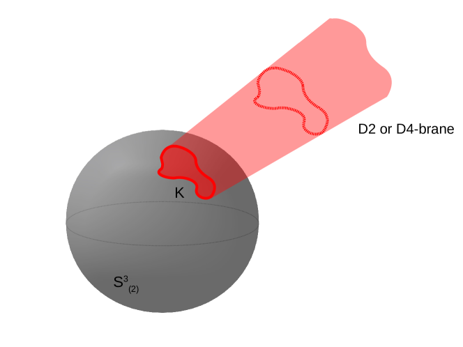
Figure 14: Knot ${\bf K}$ on D6-branes wrapped on ${\bf S}^{3}_{(2)}$ of a deformed conifold is represented by a D2-brane (or D4-brane) surface operator that intersects the D6-branes on ${\bf K}$. This picture is before geometric transition. After geometric transition, the D6-branes disappear and are replaced by fluxes on a non-Kähler resolved conifold, but the D2-brane (or D4-brane) state survives on the dual side retaining all information of the knot ${\bf K}$.

The attentive reader must have noticed the key difference between (250) and (448). The former is constructed from a modified gauge field ${\cal A}_{d}$ by combining the original gauge field ${\cal A}$ and the Coulomb branch scalars $\phi$ as in (249). For the present case, the vector multiplet has no scalars, and assuming we keep vanishing expectation values of the scalars in the chiral multiplets, the boundary theory will be constructed solely using the non-abelian gauge field ${\cal A}$, leading to (448). Quantum mechanically however the difference is only in the choices of the coupling constants for the boundary theories (250) and (448). This is because of the following path integral equivalence in the Euclidean formalism:

$$\int_{\cal C}{\cal D}{\cal A}_{d}~{}{\rm exp}\left[-S_{bnd}({\cal A}_{d})\right]~{}F({\cal A}_{d})=\int_{\cal C}{\cal D}{\cal A}~{}{\rm exp}\left[-S_{bnd}({\cal A})\right]~{}F({\cal A}),$$ (449)

where $F({\cal A})$ is any observable in the theory and ${\cal C}$ is the integration cycle. Therefore in the path integral ${\cal A}_{d}$ is just a dummy variable and can be replaced by the gauge field ${\cal A}$. Although our discussion above is a bit sloppy as we are ignoring many subtle points, the essential physics is captured in (449). For more details on the equivalence of two path integrals for both real and complex gauge fields, one may refer to section (2.4) of [11].

The three-dimensional boundary theory (448), defined on ${\bf S}^{3}_{(1)}$, remains the same when we go to the mirror type IIA side. Since the SYZ transformations [44, 45] do not change the spacetime metric, the three-cycle ${\bf S}^{3}_{(1)}$ on the type IIB side goes unchanged to the type IIA side. However the D5-branes wrapped on the two-cycle of the non-Kähler resolved confold become D6-branes wrapped on the three-cycle ${\bf S}^{3}_{(2)}$ of the non-Kähler deformed conifold. The world-volme of the D6-branes is now (395), and therefore a flop operation (396) will transfer the boundary theory (448) defined on the three-cycle ${\bf S}^{3}_{(1)}$ to the three-cycle ${\bf S}^{3}_{(2)}$ of the deformed conifold, giving us:

$$S_{ov}=\left({\widetilde{b}}_{2}+{\widetilde{c}}_{2}\right)\int_{{\bf S}^{3}_{(2)}}{\rm Tr}\left({\cal A}\wedge d{\cal A}+{2i\over 3}{\cal A}\wedge{\cal A}\wedge{\cal A}\right),$$ (450)

where, although we use the same notation of (448), ${\cal A}$ should be thought of as the gauge field defined on ${\bf S}^{3}_{(2)}$. Knots may now be inserted on ${\bf S}^{3}_{(2)}$ using D2-brane (or D4-brane) surface operators as shown in fig 14. The construction parallels the discussion in section 3.3.1 in spirit only as specific details differ. The difference of course stems from the construction of the Ooguri-Vafa model [8] starting with Table 2 compared to the construction in section 3 starting with Table 1. The flop operation (396) with the added complication of geometric transition, as well as the absence of the Coulomb branch scalars, in fact makes it harder to implement similar procedure as in section 3.3.1. We will therefore not analyze the story further and only make few observations keeping most of the details for the sequel.

The first observation is the M-theory lift of the knot configurations on ${\bf S}^{3}_{(2)}$. The uplift leads to M2-brane states in the $G_{2}$ structure manifold of the second kind associated with three T-dualities (see discussion above). These M2-brane states do not wrap the eleven-dimensional circle, so are distinct from the ones leading to non-abelian enhancement discussed for the $G_{2}$ structure manifold of the first kind associated with one T-duality. This would then be the uplift of the surface operators in M-theory.

The second observation is that the knots appearing from the surface operators do not follow similar pathway that we developed earlier in section 3.3.1 and 3.3.2 for Witten’s model [11]. This is because we cannot study the abelian version now as the model is only defined for large $N$, implying that our earlier analysis of the knots using operators ${\bf A}_{k}$, ${\bf B}_{k}$ and ${\bf C}_{(2,\sigma_{j})}$ in section 3.3.2 may not be possible now. Secondly, similar manipulations to the BHN equations that we did in section 3.3.1 now cannot be performed.

What can be done here? There is one well known procedure that we can follow. We can use the canonical quantization approach by slicing the three-cycle ${\bf S}^{3}_{(2)}$ containing the knot ${\bf K}$ into many pieces so that each piece appears locally as ${\bf S}^{2}_{(2)}\times{\bf R}$ where ${\bf S}^{2}_{(2)}$ is a two-dimensional sphere with punctures $p_{i}$’s. On every piece, the action (450) in gauge ${\cal A}_{0}=0$ gives classical solution ${\cal F}_{ij}=0$. One may compare this to the classical solution ${\cal F}_{12}=0$ that we get from (448) $-$ which in turn may be assumed to be the special case of (181) with the scalar fields switched off. The constraint implies that the physical space $\{{\cal A}\}$ to be moduli space of flat connections on the punctured sphere ${\bf S}^{2}_{(2)}$ (modulo gauge transformation) which has a finite volume. After imposing the constraint and then quantizing gives a finite dimensional Hilbert space $\mathcal{H}_{({\bf S}^{2}_{(2)},p_{i})}$, with $i=1,2,...r$, whose states are related to the $r$-point correlation functions of the Wess-Zumino-Novikov-Witten conformal field theory (WZNW model) in the two dimensional sphere ${\bf S}^{2}_{(2)}$ [55]. The WZNW model possesses level $k$ current algebra symmetry $G_{k}$ besides the conformal symmetry, where the Chern-Simons coupling $k\equiv 2\pi\left({\widetilde{b}}_{2}+{\widetilde{c}}_{2}\right)$ is identified with the level $k$ of WZNW models.

This connection between Chern-Simons theory (450) and WZNW model [2, 3] brings us to the familiar playground where a path integral of the form (449), now defined with (450), may be identified with a quantum state in the Hilbert space of WZNW model with $r$ punctures. The story can be elaborated by working out the link invariants, one example is shown in fig 15, but we will not do so here. Our aim is to find a supergravity link to this construction, and we leave this for the sequel.

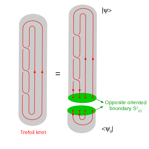
Figure 15: An example of a trefoil knot computation in the Ooguri-Vafa model. The knot invariant is now proportional to $\langle\Psi_{0}|\Psi\rangle$, which is somewhat similar in spirit with the knot invariants computed earlier. The details however differ.

The third observation is related to geometric transition in the wrapped D6-branes’ picture. Under geometric transition, the D6-branes wrapped on the three-cycle ${\bf S}^{3}_{(2)}$ of a non-Kähler deformed conifold disappear and are replaced by a non-Kähler resolved conifold with fluxes and no branes. What happens to the knot configurations on ${\bf S}^{3}_{(2)}$? This was the conundrum that we started off with in section 2.2. Introducing the D2-brane surface operators (or equivalently D4-brane surface operators) in the wrapped D6-branes’ picture now resolves the conundrum. After geometric transition, even though the D6-branes disappear, the D2-brane (or D4-brane) configurations that are responsible for the knots, as shown in fig 14, continue to survive on the resolved conifold side. Thus the gravity dual, which is our non-Kähler resolved conifold with fluxes, now equipped with the D2-brane (or D4-brane) states, continues to retain all the informations of knots and knot invariants and may be extracted with high fidelity.

5 Discussions and conclusions

In recent times we have understood that knot invariants like Jones polynomial in three-dimensional space ${\bf W}$ can be computed by understanding the solutions of certain elliptic partial differential equations in four-dimensional space ${\bf V}$, where ${\bf W}$ is the boundary of ${\bf V}$. These equations were originally derived in a topologically modified ${\cal N}=4$ Super Yang-Mills by imposing a localization condition into the Chern-Simons theory in the three-dimensional boundary ${\bf W}$ [11]. The restriction to the three-dimensional boundary was realized by switching on an axionic field in the four-dimensional gauge theory defined on ${\bf V}={\bf W}\times{\bf R}^{+}$. This way various details about knot configurations may be addressed directly using the dynamics of four-dimensional gauge theory.

In a parallel development, Ooguri-Vafa [8] studied $SU(N)$ knot invariants using a topological theory generated by wrapping D6-branes on three-cycle of a deformed conifold. Here the knot invariants may be associated to counting certain BPS configurations that have origins in the gravity dual of the wrapped D6-branes’ configuration. The gravity dual is given by resolved conifold with topological fluxes.

In the first part of our work we present an alternative derivation of the results of [11]. We show that the physics studied in both ${\bf W}$ and ${\bf V}$ can be derived from a configuration in M-theory on a certain seven-dimensional manifold with fluxes and no branes other than the M2-branes. These M2-branes serve dual purpose: one set of configurations lead to non-abelian gauge theory in ${\bf V}$; and another set of configurations lead to surface operators in ${\bf V}$ that are responsible for knots in ${\bf W}$.

Restricting the knots to the boundary ${\bf W}$ is achieved by switching on a dipole or a RR deformation in ${\bf V}$ that can be parametrized from supergravity. The M-theory uplifts leads to a seven-dimensional manifold, as mentioned above, of the form of a warped Taub-NUT space fibered over a three-dimensional base. Supergravity analysis leads to a four-dimensional Hamiltonian (167), from where a series of BPS equations are derived. A sets of these BPS equations are exactly the localization equations of [11] and [13], and we call them the BHN equations (the acronym stands for Bogomolnyi, Hitchin and Nahm). The remaining sets of the BPS equations are shown to be solved exactly using supergravity variables. Therefore one of our results was to show that such equations emerge from M-theory compactifications and their coefficients are succinctly interpreted in terms of supergravity parameters.

We also considered various types of solutions of such BHN equations alongwith their deformations. One possibility is to have codimension three solutions denoted by ’t Hooft operators. These solutions appear as opers, and we discuss them briefly here attempting a supergravity interpretation. Another possibility is to have codimension two solutions denoted by surface operators. We make a detailed study of this in our work and show how the surface operators, which we interpret as certain configuration of M2-branes, modify the BHN equations. These modifications are given by introducing delta function sources whose coefficients can be traced to the supergravity parameters in our model. Additionally we argue how the M2-brane surface operators help us to study the link invariants for various knot configurations in the abelian case.

In the second part of the paper we argue how the Ooguri-Vafa model may also be derived from a configuration in M-theory defined on a different seven-dimensional manifold that is given by another warped Taub-NUT fibered over a three-dimensional base. The warping and fluxes now are such that the supersymmetry is reduced to ${\cal N}=1$, and the seven-dimensional manifold has a $G_{2}$ structure. Nevertheless, many of the physics discussed in the first part of the paper follow a similar route in the second part too. There are crucial differences of course, which we point out in our paper. For example the topological theory is simpler now, but the analysis of knots using surface operators are harder because there is no abelian simplification that can be performed now. There is also a relocation of the knots on the three-cycle of the deformed conifold instead on the spacetime boundary ${\bf W}$ earlier. This relocation is associated to a flop transition that can be performed on the mirror type IIA side. In our opinion these are all new results.

There are a number of future directions. For example, in the first part we only studied the link invariants for the abelian case, so a natural question would to investigate the non-abelian scenario. This is harder because, as we discussed in the text, the effect of the non-abelian configuration of the surface operators on the BHN equations are difficult to handle. Thus solving the BHN equations and interpreting the knots in terms of solutions of the BHN equations in the non-abelian case will be more challenging.

For the second part we only make the barest beginnings in this direction, and leave most of the details for the sequel. For example the configuration of the surface operators in terms of M2 or M5-branes, details about the flop transition and the subsequent analysis of knot invariants still remain to be elaborated. Other connection to A-polynomial of [14], Khovanov homology [4] etc have not been touched here at all, and we expect to study them in the sequel. Thus we see that the two connections to M-theory seven-manifolds explored in this paper lead to a rich spectrum of ideas that can allow us to have a fruitful dialogue between M-theory supergravity on one hand and topological field theory and mathematics on the other.

Acknowledgements

We would like to specifically thank Edward Witten for helpful correspondences clarifying many subtleties of [11]; to Johannes Walcher for initial collaboration and for [43]; to Ori Ganor for explaining the cubic term in (17) and for other helpful comments via [23]; and to Sergei Gukov for discussions and for a helpful reference. V. E. D. is grateful to Maxim Emelin, Avinash Raju, Sam Selmani and Bala Subramanian for illuminating discussions, to Chethan Krishnan for pointing out useful references and to Jatin Panwar for invaluable help with the figures. We would also like to thank Siddharth Dwivedi, Sam Selmani, Jihye Seo and Zodinmawia for initial collaborations. The work of K. D and V. E. D is supported in part by National Science and Engineering Research Council of Canada.

References

- [1] J. W. Alexander, “Topological invariants of knots and links”, Trans. Am. Math. Soc. 30, 275 (1928); V. F. R. Jones, “A polynomial invariant for knots via von Neumann algebras”, Bull. AMS, 103 (1985); P. Freyd, D. Yetter, J. Hoste, W. B. R. Lickorish, K. Millet and A. Ocneanu, “A new polynomial invariant of knots and links”, Bull. AMS.12(1985) 239; J. H. Przytycki and K. P. Traczyk, “Invariants of links of Conway Type”, Kobe J. Math. 4, 115 (1987); L. H. Kauffman, “An invariant of regular isotopy”, Trans. Amer. Math. Soc. 318, 417 (1990).
- [2] E. Witten, “Quantum Field Theory and the Jones Polynomial,” Commun. Math. Phys. 121, 351 (1989).
- [3] P. Ramadevi, T. R. Govindarajan and R. K. Kaul, “Three-dimensional Chern-Simons theory as a theory of knots and links. 3. Compact semisimple group”, Nucl. Phys. B 402, 548 (1993) [hep-th/9212110]
- [4] M. Khovanov, “A categorification of the Jones polynomial”, Duke Math. J. 3, 359 (2000).
- [5] M. Khovanov, “ link homology”, Algebr. Geom. Topol. 4, 1045 (2004).
- [6] M. Khovanov and L. Rozansky, “Matrix factorizations and link homology”, Fund. Math. 199, 1 (2008).
- [7] R. Gopakumar and C. Vafa, “On the gauge theory / geometry correspondence,” Adv. Theor. Math. Phys. 3, 1415 (1999) [hep-th/9811131].
- [8] H. Ooguri and C. Vafa, “Knot invariants and topological strings,” Nucl. Phys. B 577, 419 (2000) [hep-th/9912123].
- [9] J. M. F. Labastida and M. Marino, “Polynomial invariants for torus knots and topological strings,” Commun. Math. Phys. 217, 423 (2001) [hep-th/0004196]; P. Ramadevi and T. Sarkar, “On link invariants and topological string amplitudes,” Nucl. Phys. B 600, 487 (2001) [hep-th/0009188].
- [10] S. Gukov, A. S. Schwarz and C. Vafa, “Khovanov-Rozansky homology and topological strings,” Lett. Math. Phys. 74, 53 (2005) [hep-th/0412243].
- [11] E. Witten, “Fivebranes and Knots,” arXiv:1101.3216 [hep-th].
- [12] A. Kapustin and E. Witten, “Electric-Magnetic Duality And The Geometric Langlands Program,” Commun. Num. Theor. Phys. 1, 1 (2007) [hep-th/0604151].
- [13] D. Gaiotto and E. Witten, “Knot Invariants from Four-Dimensional Gauge Theory,” Adv. Theor. Math. Phys. 16, no. 3, 935 (2012) [arXiv:1106.4789 [hep-th]].
- [14] M. Aganagic and C. Vafa, “Large N Duality, Mirror Symmetry, and a Q-deformed A-polynomial for Knots,” arXiv:1204.4709 [hep-th].
- [15] V. Errasti Díez, “A companion to Knot Invariants and M-Theory I: Proofs and Derivations,” To appear.
- [16] K. Dasgupta, K. Oh and R. Tatar, “Geometric transition, large N dualities and MQCD dynamics,” Nucl. Phys. B 610, 331 (2001) [hep-th/0105066].
- [17] K. Dasgupta, K. Oh and R. Tatar, “Open / closed string dualities and Seiberg duality from geometric transitions in M theory,” JHEP 0208, 026 (2002) [hep-th/0106040].
- [18] M. Bershadsky, C. Vafa and V. Sadov, “D strings on D manifolds,” Nucl. Phys. B 463, 398 (1996) [hep-th/9510225].
- [19] K. Dasgupta and S. Mukhi, “Brane constructions, fractional branes and Anti-de Sitter domain walls,” JHEP 9907, 008 (1999) [hep-th/9904131].
- [20] A. M. Uranga, “Brane configurations for branes at conifolds,” JHEP 9901, 022 (1999) [hep-th/9811004].
- [21] K. Dasgupta and S. Mukhi, “Brane constructions, conifolds and M theory,” Nucl. Phys. B 551, 204 (1999) [hep-th/9811139].
- [22] K. M. Lee and H. U. Yee, “BPS String Webs in the 6-dim (2,0) Theories,” JHEP 0703, 057 (2007) [hep-th/0606150].
- [23] O. Ganor, “A derivation of the term in eqn. (17) and in [11],” Nov 2015.
- [24] A. Bergman and O. J. Ganor, “Dipoles, twists and noncommutative gauge theory,” JHEP 0010, 018 (2000) [hep-th/0008030].
- [25] K. Dasgupta, O. J. Ganor and G. Rajesh, “Vector deformations of N=4 superYang-Mills theory, pinned branes, and arched strings,” JHEP 0104, 034 (2001) [hep-th/0010072].
- [26] A. Bergman, K. Dasgupta, O. J. Ganor, J. L. Karczmarek and G. Rajesh, “Nonlocal field theories and their gravity duals,” Phys. Rev. D 65, 066005 (2002) [hep-th/0103090].
- [27] Y. Imamura, “Born-Infeld action and Chern-Simons term from Kaluza-Klein monopole in M theory,” Phys. Lett. B 414, 242 (1997) [hep-th/9706144]; A. Sen, “Dynamics of multiple Kaluza-Klein monopoles in M and string theory,” Adv. Theor. Math. Phys. 1, 115 (1998) [hep-th/9707042]; “A Note on enhanced gauge symmetries in M and string theory,” JHEP 9709, 001 (1997) [hep-th/9707123]; K. Becker, M. Becker, K. Dasgupta and P. S. Green, “Compactifications of heterotic theory on nonKahler complex manifolds. 1.,” JHEP 0304, 007 (2003) [hep-th/0301161].
- [28] W. Fischler and A. Rajaraman, “M(atrix) string theory on K3,” Phys. Lett. B 411, 53 (1997) [hep-th/9704123].
- [29] A. Hanany and G. Lifschytz, “M(atrix) theory on T**6 and a m(atrix) theory description of K K monopoles,” Nucl. Phys. B 519, 195 (1998) [hep-th/9708037].
- [30] R. C. Myers, “Dielectric branes,” JHEP 9912, 022 (1999) [hep-th/9910053].
- [31] J. Bagger and N. Lambert, “Modeling Multiple M2’s,” Phys. Rev. D 75, 045020 (2007) [hep-th/0611108]; “Gauge symmetry and supersymmetry of multiple M2-branes,” Phys. Rev. D 77, 065008 (2008) [arXiv:0711.0955 [hep-th]]; J. Bagger, N. Lambert, S. Mukhi and C. Papageorgakis, “Multiple Membranes in M-theory,” Phys. Rept. 527, 1 (2013) [arXiv:1203.3546 [hep-th]].
- [32] S. Gukov and E. Witten, “Gauge Theory, Ramification, And The Geometric Langlands Program,” hep-th/0612073.
- [33] S. Gukov and E. Witten, “Rigid Surface Operators,” Adv. Theor. Math. Phys. 14, no. 1, 87 (2010) [arXiv:0804.1561 [hep-th]].
- [34] S. Gukov, “Surface Operators,” arXiv:1412.7127 [hep-th].
- [35] E. Witten, “Small instantons in string theory,” Nucl. Phys. B 460, 541 (1996) [hep-th/9511030].
- [36] S. Gukov, “Gauge theory and knot homologies,” Fortsch. Phys. 55, 473 (2007) [arXiv:0706.2369 [hep-th]].
- [37] E. Witten, “Analytic Continuation Of Chern-Simons Theory,” AMS/IP Stud. Adv. Math. 50, 347 (2011) [arXiv:1001.2933 [hep-th]].
- [38] R. Dijkgraaf, S. Gukov, A. Neitzke and C. Vafa, “Topological M-theory as unification of form theories of gravity,” Adv. Theor. Math. Phys. 9, no. 4, 603 (2005) [hep-th/0411073].
- [39] M. Marino, “Chern-Simons theory, Matrix Models, and Topological Strings,” Int. Ser. Monogr. Phys. 131, 1 (2005).
- [40] K. Dasgupta, M. Emelin and E. McDonough, “Non-Kahler Resolved Conifold, Localized Fluxes in M-Theory and Supersymmetry,” JHEP 1502, 179 (2015), [arXiv:1412.3123 [hep-th]].
- [41] J. Maldacena and D. Martelli, “The Unwarped, resolved, deformed conifold: Fivebranes and the baryonic branch of the Klebanov-Strassler theory,” JHEP 1001, 104 (2010) [arXiv:0906.0591 [hep-th]].
- [42] C. Faber and R. Pandharipande, “Hodge Integrals and Gromov-Witten Theory”, math.AG/9810173.
- [43] J. Walcher, “Goods to those who wait”, private email correspondence, April 2013.
- [44] A. Strominger, S. T. Yau and E. Zaslow, “Mirror symmetry is T duality,” Nucl. Phys. B 479, 243 (1996) [hep-th/9606040].
- [45] M. Becker, K. Dasgupta, A. Knauf and R. Tatar, “Geometric transitions, flops and nonKahler manifolds. I.,” Nucl. Phys. B 702, 207 (2004) [hep-th/0403288]; S. Alexander, K. Becker, M. Becker, K. Dasgupta, A. Knauf and R. Tatar, “In the realm of the geometric transitions,” Nucl. Phys. B 704, 231 (2005) [hep-th/0408192]; M. Becker, K. Dasgupta, S. H. Katz, A. Knauf and R. Tatar, “Geometric transitions, flops and non-Kahler manifolds. II.,” Nucl. Phys. B 738, 124 (2006) [hep-th/0511099].
- [46] F. Chen, K. Dasgupta, J. M. Lapan, J. Seo and R. Tatar, “Gauge/Gravity Duality in Heterotic String Theory,” Phys. Rev. D 88, 066003 (2013) [arXiv:1303.4750 [hep-th]].
- [47] F. Chen, K. Dasgupta, P. Franche, S. Katz and R. Tatar, “Supersymmetric Configurations, Geometric Transitions and New Non-Kahler Manifolds,” Nucl. Phys. B 852, 553 (2011) [arXiv:1007.5316 [hep-th]].
- [48] K. Dasgupta, M. Grisaru, R. Gwyn, S. H. Katz, A. Knauf and R. Tatar, “Gauge-Gravity Dualities, Dipoles and New Non-Kahler Manifolds,” Nucl. Phys. B 755, 21 (2006) [hep-th/0605201].
- [49] S. Chiossi and S. Salamon, “The Intrinsic torsion of SU(3) and G(2) structures,” [math/0202282 [math-dg]].
- [50] G. Lopes Cardoso, G. Curio, G. Dall’Agata, D. Lust, P. Manousselis and G. Zoupanos, “Non-Kähler string backgrounds and their five torsion classes,” Nucl. Phys. B 652, 5 (2003) [hep-th/0211118].
- [51] S. Gurrieri, J. Louis, A. Micu and D. Waldram, “Mirror symmetry in generalized Calabi-Yau compactifications,” Nucl. Phys. B 654, 61 (2003) [hep-th/0211102].
- [52] J. P. Gauntlett, D. Martelli and D. Waldram, “Superstrings with intrinsic torsion,” Phys. Rev. D 69, 086002 (2004) [hep-th/0302158].
- [53] K. Dasgupta and M. M. Sheikh-Jabbari, “Noncommutative dipole field theories,” JHEP 0202, 002 (2002) [hep-th/0112064].
- [54] K. Dasgupta and M. Shmakova, “On branes and oriented B fields,” Nucl. Phys. B 675, 205 (2003) [hep-th/0306030].
- [55] J. Wess and B. Zumino, “Consequences of anomalous Ward identities,” Phys. Lett. B 37, 95 (1971); E. Witten, “Global Aspects of Current Algebra,” Nucl. Phys. B 223, 422 (1983); S. P. Novikov, “The Hamiltonian formalism and a many valued analog of Morse theory,” Usp. Mat. Nauk 37N5, no. 5, 3 (1982) [Russ. Math. Surveys 37, no. 5, 1 (1982)].