Signatures of Young Planets
in the Continuum Emission From Protostellar Disks

Abstract

Many protostellar disks show central cavities, rings, or spiral arms likely caused by low-mass stellar or planetary companions, yet few such features are conclusively tied to bodies embedded in the disks. We note that even small features on the disk’s surface cast shadows, because the starlight grazes the surface. We therefore focus on accurately computing the disk’s thickness, which depends on its temperature. We present models with temperatures set by the balance between starlight heating and radiative cooling, that are also in vertical hydrostatic equilibrium. The planet has 20, 100, or 1000 M_⊕, ranging from barely enough to perturb the disk significantly, to clearing a deep tidal gap. The hydrostatic balance strikingly alters the model disk’s appearance. The planet-carved gap’s outer wall puffs up under starlight heating, throwing a shadow across the disk beyond. The shadow appears in scattered light as a dark ring that could be mistaken for a gap opened by another more distant planet. The surface brightness contrast between outer wall and shadow for the 1000-M_⊕ planet is an order of magnitude greater than a model neglecting the temperature disturbances. The shadow is so deep it largely hides the planet-launched spiral wave’s outer arm. Temperature gradients are such that outer low-mass planets undergoing orbital migration will converge within the shadow. Furthermore the temperature perturbations affect the shape, size, and contrast of features at millimeter and centimeter wavelengths. Thus radiative heating and cooling are key to the appearance of protostellar disks with embedded planets.

1 Introduction

Extrasolar planetary systems are now known to be strikingly diverse in the member planets’ masses, multiplicities and orbital configurations (Udry & Santos, 2007; Batalha et al., 2013; Laughlin & Lissauer, 2015; Winn & Fabrycky, 2015). Placing our Solar system in the context of these new discoveries will require learning how the diversity arises from differing conditions or processes in the protostellar disks that gave the planets birth. A promising way forward is by studying spatially resolved observations of the protostellar disks orbiting nearby young stars, which reveal numerous features in the emission from the dust and gas: central cavities, bright and dark rings, including asymmetric ones, and spiral arms. These features are qualitatively consistent with gravitational perturbation by low-mass stellar or planetary companions, and offer an opportunity to learn about the early stages of planet and star formation within the disks.

Clear examples of the variety of structures found in protostellar disks are around the young stars SAO 206462 (also known as HD135344B), J160421.7–213028 (hereafter J1604), and TW Hya. The first two disks have large ($>$10 AU) cavities that are dark in the continuum emission from millimeter and centimeter-size grains. While SAO 206462 shows horseshoe-shaped azimuthal asymmetries (Pérez et al., 2014; van der Marel et al., 2016), J1604 is characterized by an almost axisymmetric narrow ring at millimeter wavelengths (Zhang et al., 2014; Dong et al., 2017). In the optical and near-infrared, the SAO 206462 disk shows a well-defined $m=2$ spiral design (Muto et al., 2012), while the surface brightness around J1604 is circularly symmetric (Mayama et al., 2012a; Thalmann et al., 2010), similar in shape to the millimeter wavelengths. Unlike SAO 206462 and J1604, the TW Hya disk at 0.85 mm shows a series of at least five narrow concentric rings extending from 1 to 50 AU (Andrews et al., 2016). Near-infrared imaging also shows rings, but these are much wider and only loosely related to those observed in the sub-millimeter (van Boekel et al., 2017).

The dynamical interaction between the circumstellar material and planets or low-mass stellar companions is the most widely discussed explanation for the observed structures. This is because, on one hand, circular gaps, spiral waves, and azimuthal asymmetries are naturally produced by the gravitational interaction with one or more companions (Li et al., 2000a; Baruteau et al., 2014; Kley & Nelson, 2012), and on the other hand, the search for exoplanets has revealed that most mature stars host one or more planets, therefore many protostellar disks should show the effects of planet formation.

Recent observations however point to major discrepancies with planet-disk interaction models. For example, the infrared spiral arms observed in SAO 206462 and MWC 758 have large opening angles, which, if interpreted as the manifestation of density waves propagating away from an embedded planet at the local sound speed, imply temperatures much higher than equilibrium with the stellar radiation field (Benisty et al., 2015). Furthermore, Juhász et al. (2015) pointed out that the appearance of the spiral structures in scattered light requires disk pressure scale heights several times larger than expected under hydrostatic equilibrium. Finally, some models used to interpret the observed spiral features lack internal consistency. As an example, planet masses of several Jupiters were derived in the case of SAO 206462 by adopting prescriptions for the disk-planet interaction that hold only for planets with masses less than 1 Earth. In contrast, the rather simple morphologies of the J1604 and LkCa 15 disks, and even the multi-ring morphology in TW Hya, HL Tau, HD 163296, and AS 209 can be explained using planet-disk interaction models (Dong et al., 2015c; Picogna & Kley, 2015; Pinilla et al., 2015; Jang-Condell & Turner, 2013; Jin et al., 2016; Isella et al., 2016; Fedele et al., 2017). Furthermore, a candidate young planet has been imaged in the dust-depleted cavity of LkCa 15 (Sallum et al., 2015). Based on this sample, we might argue that the features in “dynamically cold” ring-like disks result from planet-disk interaction, while those in “dynamically hot” asymmetric disks come from other yet unknown physical processes.

Improving our understanding of planet-disk interaction requires both enlarging the still small and biased sample of disks observed at high angular resolution, and improving upon theoretical models of the disks’ response to perturbations from stellar and planetary companions. In this paper we address the modeling issue, motivated by the fact that current treatments of embedded planets’ effects on the disk’s appearance involve very simple prescriptions for the disk’s thermal response. Juhász et al. (2015) noted that spiral structures in the scattered light are more sensitive to disturbances in the disk’s pressure scale height than to disturbances in the density. The scale height is proportional to the sound speed and thus depends on the temperature. The temperature in turn is highly sensitive to the angle of incidence of the starlight, so accurately calculating the shape of the disk surface is crucial for modeling the system’s appearance (Jang-Condell, 2008).

To address these issues, we investigate the planet-disk interaction’s effects on the disk temperature and density. We construct models that are in hydrostatic equilibrium in the vertical direction, with temperatures set by the balance between starlight heating and radiative cooling. Two-dimensional hydrodynamical calculations in the equatorial plane yield surface density maps, which we expand into three-dimensional density distributions using the hydrostatic equilibrium for the initially guessed temperature distribution. We compute new temperatures using detailed frequency-dependent Monte Carlo radiative transfer calculations treating scattering, absorption and thermal re-emission. We then step forward in time, letting each patch of the disk expand or contract vertically on its own thermal or dynamical timescale, and again compute temperatures accounting for the way the starlight falls across the disk’s new shape. The calculations continue as long as needed to reach joint radiative and hydrostatic equilibrium. This modeling approach is laid out in section 2, and we describe its results in section 3. We find that planets affect the temperatures through the interplay between starlight heating, the disk’s shape, and radiative cooling. We then apply the model to investigate the planet-induced perturbations’ observational appearance. We focus on signatures in infrared scattered light, which trace the disk’s surface layers, and in millimeter-wave dust continuum emission, which trace the dust in the midplane. Section 4 deals with the temperature structures’ implications for disks’ equation of state and planets’ orbital migration. The models’ relationship to the features observed in protostellar disks is discussed in section 5, and the conclusions are presented in section 6.

2 Modeling the Planet-Disk Interaction

Accurately modeling the planet-disk interaction requires solving the following problem. The orbiting planet exerts a gravitational force on nearby disk material, launching acoustic waves which compress and rarefy the gas through which they pass, perturbing the surface density. The density fluctuations alter the height and slope of the surface where the illuminating starlight is absorbed. Large enough excursions of the surface cast shadows across the disk beyond. The changing illumination is reflected in the system’s appearance in scattered light. Over the heating or cooling timescale, the changing illumination also affects the interior temperatures, which feed back on the acoustic waves’ own propagation. Furthermore, planets more massive than Jupiter launch waves strong enough to clear disk material from an annulus around the planetary orbit. This drastic change in the disk structure further alters how starlight is absorbed and scattered across the disk.

Several approximations are necessary to make this problem tractable. To begin with, we assume that the planet disturbs the disk in a way that depends weakly on the temperature, so we can solve for the gas dynamics using temperatures differing from those we will eventually determine through detailed Monte Carlo radiative transfer. We find that this is valid for planets too low in mass to open a gap in the disk. However the formation of a gap leads to large temperature excursions, making the approximation questionable. We nevertheless separate the dynamics and radiative transfer because the latter takes far too much computer time to be carried out with each hydrodynamical time step. Frequency-averaged semi-analytic transfer methods are much faster (Jang-Condell, 2009) and adequately reproduce the results of detailed transfer calculations (Jang-Condell & Turner, 2012), but have not been combined with the 3-D hydrodynamical methods needed to model the surface-illuminated disk’s non-axisymmetric response to an embedded planet. Numerical 3-D radiation hydrodynamics modeling is now feasible in the flux-limited diffusion approximation, including direct starlight treated by integrating along radial rays (Kuiper et al., 2010; Bitsch & Kley, 2011; Flock et al., 2013), but the flux-limiting yields wrong answers when shadowing is important (Hayes & Norman, 2003), and these approaches also neglect scattered starlight. In contrast, the Monte Carlo approach finds the radiation field’s full dependence on both angle and frequency. Thus the models for gap-opening planets presented below, despite their limitations, provide insights into the appearance of disks with embedded planets that are not available from other existing results.

2.1 Unperturbed Disk

We start our investigation by adopting a disk model unperturbed by any planet, with gas surface density

$$\Sigma_{g}^{0}(r)=18\ \textrm{g cm}^{-2}\times\left(\frac{r}{10\textrm{AU}}\right)^{-1}$$ (1)

extending from 0.1 AU to 50 AU. Its total mass is 0.007 $M_{\odot}$, less than the minimum-mass Solar nebula but consistent with the masses of young disks in nearby star forming regions (e.g. Andrews & Williams, 2007; Isella et al., 2009).

The central star has a mass of 1 $M_{\sun}$, a luminosity of 1 $L_{\sun}$, and an effective temperature of 5600 K. The disk temperature and vertical density structure are calculated under the assumption of hydrostatic equilibrium between the gas pressure and the stellar gravity. Dust is well-mixed throughout the gas, with a uniform gas-to-dust ratio of 100. The interaction between dust and gas is further discussed in Section 2.3. Temperatures are computed using the Monte Carlo radiative transfer code RADMC-3D. The disk is placed in radiative equilibrium, so that the bolometric emission from each grid cell matches the rate at which starlight and other incident radiation are absorbed, following the procedure discussed in Section 2.4.

The midplane temperature of the resulting unperturbed disk model is well approximated by the power-law fit

$$T_{m}^{0}(r)\simeq\textrm{41}\textrm{K}\times\left(\frac{r}{10\textrm{AU}}\right)^{-0.45}.$$ (2)

The temperature along the direction perpendicular to the midplane is equal to $T_{m}^{0}(r)$ for $z/r<h/r\approx 0.04$. At greater heights the temperature increases to reach that of a dust grain in optically thin surroundings exposed to the starlight, $T_{s}^{0}(r)\simeq 124\,\textrm{K}(r/10\textrm{AU})^{-1/2}$ (e.g. Dullemond et al., 2001; Dullemond & Dominik, 2004).

Since most of the disk’s mass lies in the vertically-isothermal interior, the vertical density profile to first approximation is the Gaussian

$$\rho(r,z)=\frac{\Sigma(r)}{\sqrt{2\pi}h(r)}\exp\frac{-z^{2}}{2h^{2}(r)}.$$ (3)

At hydrostatic equilibrium, the pressure scale height $h(r)$ is equal to $c_{s}(r)/\Omega(r)$, where $c_{s}(r)=\sqrt{k_{b}T(r)/\mu m_{p}}$ is the isothermal gas sound speed, and $\Omega(r)=\sqrt{GM_{\star}/r^{3}}$ is the Keplerian angular speed. Using the gas temperature from Equation 2 and a mean molecular weight $\mu=2.3$, the sound speed and pressure scale height are

$$c^{0}_{s}(r)\simeq 0.38\ \textrm{km s}^{-1}\times\left(\frac{r}{10\textrm{AU}}\right)^{-0.225}$$ (4)

and

$$h^{0}(r)\simeq 0.41\textrm{AU}\times\left(\frac{r}{10\textrm{AU}}\right)^{1.275}.$$ (5)

Below we use the fits in Equations 1 and 2 as baselines against which to compare the structure of model disks perturbed by planets.

2.2 Planets Perturbing the Disk

The first step in producing synthetic images of a disk interacting with an embedded planet is to map the perturbations in the surface density. If the planet is low-mass, the perturbations are small and can be calculated by linearizing the equations of motion and continuity (Goldreich & Tremaine, 1978). In contrast, high-mass planets induce non-linear perturbations that must be investigated using numerical simulations (Bryden et al., 1999). The transition between these two regimes occurs when non-linear effects, such as shocks, become relevant in transferring the angular momentum carried by the waves into the gas (Goodman & Rafikov, 2001).

The transition from linear to non-linear perturbations in a Keplerian disk occurs around the thermal mass $M_{th}=2c_{s}^{3}/3\Omega G$ (Goodman & Rafikov, 2001; Dong et al., 2011). A planet with mass $M_{p}=M_{th}$ has a Hill sphere whose radius is comparable to the disk’s pressure scale height. In an inviscid disk, $M_{th}$ is the mass at which planets start to open annular gaps in the surrounding gas by depositing angular momentum at their innermost Lindblad resonance (Lin & Papaloizou, 1993).

For the unperturbed disk model described above, the critical mass is

$$M_{th}\sim 15M_{\oplus}\times\left(\frac{r}{\textrm{10AU}}\right)^{0.825}.$$ (6)

If $M_{p}\ll M_{th}$, the planet perturbation’s waveform can be written in polar coordinates as

$$\phi=\phi_{p}+\textrm{sign}(r-r_{p})\frac{r_{p}}{h_{p}}\times 4\left[\left(\frac{r}{r_{p}}\right)^{-0.275}+\frac{1}{5}\left(\frac{r}{r_{p}}\right)^{1.225}-1.48\right],$$ (7)

where $\phi_{0}$ is the planet’s position angle and $h_{p}$ is the pressure scale height at the planet’s orbital radius $r_{p}$. This equation was derived from Rafikov (2002) Equation 44 using a power law index for the sound speed $\nu=0.225$, as in Equation 4. In the linear regime, the perturbation is a one-armed spiral propagating from the planet both inward and outward and characterized by an opening angle depending only on the sound speed. The density perturbation’s maximum amplitude $\delta\Sigma/\Sigma_{0}\simeq M_{p}/M_{th}\ll 1$, where $\Sigma_{0}$ is the unperturbed surface density profile.

If $M_{p}\geq M_{th}$, the density perturbations induced by the planet must be calculated by numerically solving the hydrodynamics equations. In this paper, we employ the publicly available code FARGO3D (Masset, 2000, http://fargo.in2p3.fr) to simulate the disk’s interaction with planets having masses of 20, 100 and 1000 $M_{\oplus}$, corresponding to about 1.3, 7 and 70 times the thermal mass respectively. Henceforth, we refer to these three hydrodynamical results as P20, P100, and P1000, respectively. We arbitrarily place the planets at 10 AU so that the perturbations on the disk structure have spatial scales observable with current infrared and millimeter-wave telescopes. The calculations are two-dimensional in the orbital plane, with the disk structure averaged over the perpendicular direction. The code setup is described in appendix A.

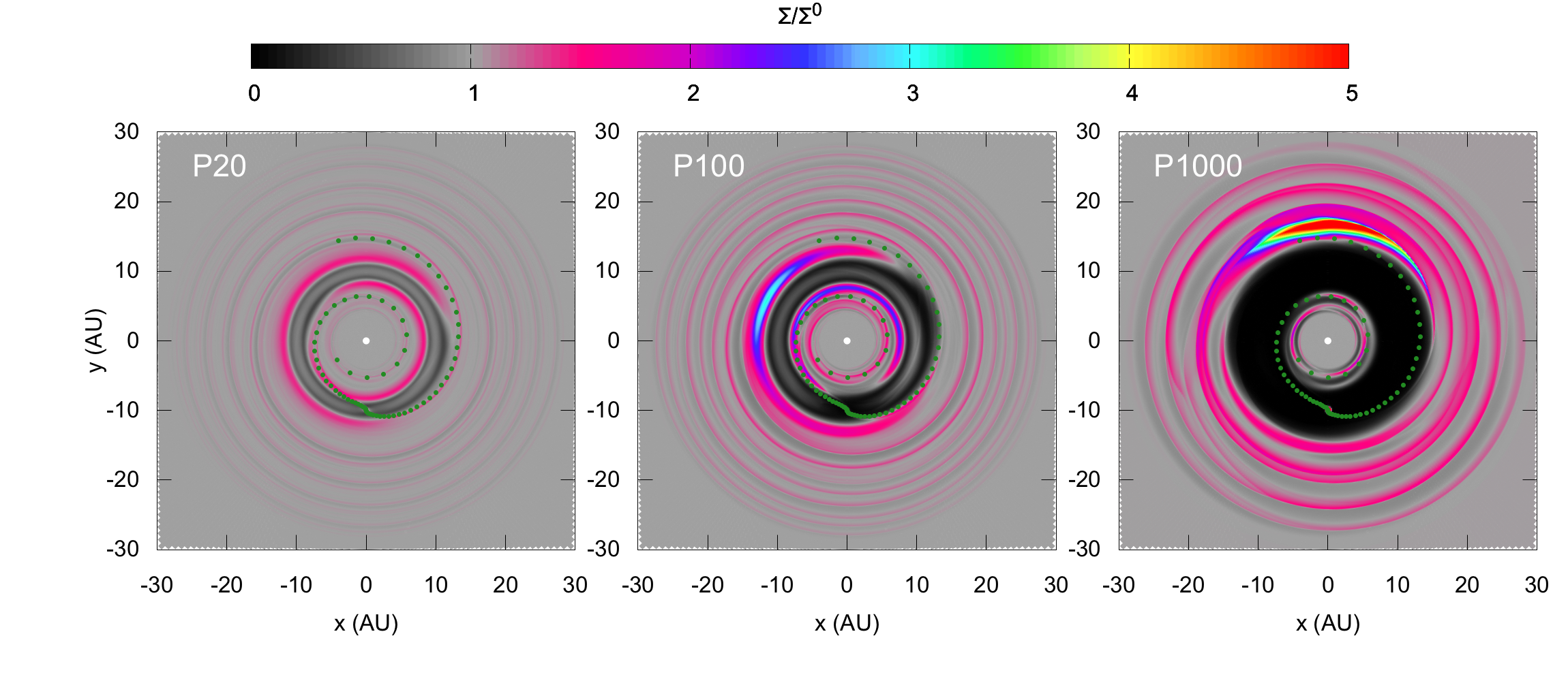
Figure 1: Surface density perturbations induced by planets of 20 (P20), 100 (P100) and 1000 (P1000) M_⊕ (left, center, and right panels, respectively) orbiting 10 AU from the star, after about 300 planet orbits ($\sim 10^{4}$ yr). The color scale shows the amplitude of the perturbations $\Sigma/\Sigma^{0}$, relative to initial surface density profile $\Sigma^{0}$ defined by Equation 1. Green dots show the locus of the peak of the spiral density wave from the linear theory (Equation 7).

In Figure 1 are snapshots of the surface density in the P20, P100, and P1000 models after 300 orbits of the planet. To highlight the perturbations, we plot the ratio of the gas surface density to that of the unperturbed disk defined by Equation 1. In the P20 model ($M_{p}\sim M_{th}$), the planet creates an $m=1$ spiral wave, similar in shape and amplitude to the linear solution of Equation 7. Furthermore, the planet partially depletes a circular gap, reducing the surface density to about half its initial value over an annulus about 3 AU wide. Near the gap’s inner and outer edges are horseshoe structures in which the surface density varies by about 40% with azimuth.

More massive planets lead to stronger density perturbations. The gap is wider and more highly depleted, the spiral density wave has a higher amplitude and deviates more from the linear solution, and the azimuthal asymmetries grow. The non-axisymmetric structures take the form of anticyclonic vortices (Li et al., 2000b). It is worth noting that while spiral density waves rotate at the planet’s Keplerian speed, the vortices formed at the gap edges rotate at the local orbital speed. This difference could profoundly impact the coupling between dust and gas, the disk thermal structure, and therefore the observability of such perturbations.

Finally, we point out that our hydrodynamic simulations’ outcomes depend on poorly known physical quantities such as the accretion stresses, as well as numerical parameters such as the smoothing length applied to the planet’s gravitational potential (see appendix A). Investigating the interplay of these parameters is not the purpose of this paper. Instead, we use FARGO3D simply as a tool to produce surface density maps showing features similar to those observed in protostellar disks, namely, circular gaps, azimuthal asymmetries, and spiral density waves.

2.3 Dynamical Coupling Between Dust and Gas

While the planet-disk interaction affects the distribution of circumstellar gas, the bulk of the disk’s opacity is carried by dust grains. The perturbations that planets induce on the disk temperature and continuum emission therefore depend on the relative distributions of dust and gas. The two are coupled by drag forces over the stopping time $\tau_{s}$, which in the case of a Keplerian disk in hydrostatic equilibrium, can be written as

$$\tau_{s}\approx{2\rho_{i}a\over\Sigma\Omega}\sim 1.1\textrm{yr}\times\left(\frac{a}{1\mathrm{cm}}\right)\left(\frac{r}{10\textrm{AU}}\right)^{5/2}$$ (8)

(e.g., the review by Testi et al., 2014), where $a$ is the particle size and $\rho_{i}$ is the grains’ internal density. The right-hand form of the equation results from adopting a grain density of 2 g cm^-3 and the surface density profile in Equation 1. The stopping time increases linearly with the grain size, so small particles are more closely coupled to the gas than big ones. To quantify the effect of planet perturbations on particles of different sizes, we compare the stopping time $\tau_{s}$ to the characteristic time scale for density perturbations $\tau_{e}$ calculated as follows. Spiral waves excited by a planet rotate at the Keplerian speed $\Omega_{p}=\sqrt{GM_{\star}/r_{p}^{3}}$. The relative angular speed between the spiral perturbation and a grain orbiting at a distance $r$ from the star is therefore

$$\delta\Omega(r)=\Omega(r)-\Omega_{p}=\sqrt{GM_{\star}}\left(\frac{1}{r^{3/2}}-\frac{1}{r_{p}^{3/2}}\right).$$ (9)

If the density perturbation has a characteristic angular width $\delta\phi$, then during each orbit, a dust grain is entrained in the density wave only for the characteristic time

$$\tau_{e}\simeq\frac{\delta\phi}{\delta\Omega}=\frac{\delta\phi}{\sqrt{GM_{\star}}}\left|\frac{1}{r^{3/2}}-\frac{1}{r_{p}^{3/2}}\right|^{-1}.$$ (10)

Particles with $\tau_{s}\ll\tau_{e}$ will be distributed in the same way as the gas. If the gas surface density increases by $\delta\Sigma$, the dust surface density will simultaneously increase by the same proportion. Particles with $\tau_{s}\gg\tau_{e}$ on the other hand will not respond to the gas density variations. In between is the critical grain size $a_{cr}$, at which $\tau_{s}=\tau_{e}$. Particles smaller than $a_{cr}$ trace the gas disturbances, while larger particle are free to respond to forces other than the gas drag. Using Equation 8 and 10, we write the critical grain size as

$$a_{cr}(r)=\delta\phi\times\frac{\Sigma(r)}{2\rho_{i}}\times\left|1-\left(\frac{r}{r_{p}}\right)^{3/2}\right|^{-1}\simeq 0.8\ \textrm{cm}\times\left(\frac{10{\textrm{AU}}}{r}\right)\times\left|1-\left(\frac{r}{r_{p}}\right)^{3/2}\right|^{-1},$$ (11)

where in writing the rightmost form, we assumed $\delta\phi=10$°. Figure 2 shows $a_{cr}$ for $r_{p}=10$ AU and $\delta\phi=5$, 10 and 15°. The critical grain size at 20 AU and 40 AU from the star ranges from 0.1 to 0.3 and 0.01 to 0.03 cm, respectively. This suggests that the grains dominating the cm- and mm-wave continuum emission will trace spiral density waves generated by a planet only close to the planet itself. Micron-sized particles, which are much smaller than the critical size, are well coupled to these perturbations throughout the disk.

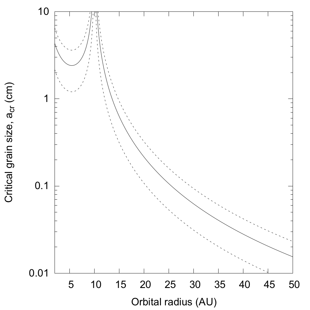
Figure 2: Critical dust particle size vs. distance from the star, for a planet orbiting at 10 AU. Only particles smaller than $a_{cr}$ couple to spiral density perturbations raised by the planet. The solid line corresponds to an angular extent for the perturbation $\delta\phi=10^{\circ}$, and the upper and lower dashed lines to $\delta\phi=15^{\circ}$ and $\delta\phi=5^{\circ}$, respectively.

The formation of gas-depleted gaps and vortices also affects the distribution of the dust relative to the gas. A gap’s outer edge is a local maximum in the gas pressure, and thus traps dust particles (Haghighipour & Boss, 2003). Trapping is most efficient for particles with Stokes number $St=\tau_{s}\Omega\simeq 2\rho_{i}a/\Sigma$ close to unity. With the surface density profile in Equation 1, $St=1$ corresponds to a grain size $a(St=1)=4.5\ \textrm{cm}\times(r/10\textrm{AU})^{-1}$. A gap’s outer edge will therefore preferentially trap cm- and mm-sized particles, while micron-sized dust remains coupled to the gas. Similarly, the gas pressure maxima at the centers of the vortices that develop on the gap’s outer edge preferentially concentrate large dust particles (Lyra et al., 2009; Birnstiel et al., 2013).

In summary, dust grains smaller than a few microns are likely to be well coupled to the gas through drag forces even in the presence of time-variable perturbations like those created by a planet. These small grains carry most of the opacity at optical and infrared wavelengths, and therefore control the starlight absorption and the disk’s temperature. However the continuum emission at mm and cm wavelengths comes from dust particles that are big enough to decouple from the gas. Thus, combining spatially-resolved observations of the gas and dust continuum emission at near-infrared and mm to cm wavelengths can potentially reveal both planet signatures and the dynamics of the larger particles.

2.4 Calculating Temperatures in Disks Perturbed by Planets

In this section, we describe the approach we adopt to compute the temperatures in disks perturbed by planets. We start by assuming that the disk beyond a few AU is heated only by the starlight. Accretion heating is neglected, which is a good approximation outside 1 AU for mass accretion rates less than about $10^{-8}$ M_⊙ yr^-1 (D’Alessio et al., 1998). We also assume that shock and compression heating related to the planet perturbations are negligible compared to the starlight heating. In this limit, the temperatures depend on the vertical distribution of dust particles smaller than a few $\mu$m, which dominate the opacity at optical and infrared wavelengths. Following the discussion of the previous section, we assume these particles are dynamically well-coupled to the gas. We take the dust and gas temperatures to be equal, which is a good approximation at vertical visual extinctions $A_{V}$ greater than about 0.1 magnitude (Dullemond et al., 2007).

For smooth surface density profiles like that of Equation 1, the balance between gas pressure and stellar gravity leads to a hydrostatic equilibrium solution in which the disk’s top and bottom surfaces are concave, bending upward with increasing distance from the star. The temperature and the pressure scale height follow radial power-laws similar to Equations 2-5 (Chiang & Goldreich, 1997; D’Alessio et al., 1998; Dullemond et al., 2001). By contrast, disks with non-monotonic surface density profiles like those resulting from disk-planet interactions have had their temperatures calculated only in a few cases. Turner et al. (2012) examined Jupiter’s effects on the Solar Nebula, finding that the gap opened by the planet was up to twice as hot as the same location in an unperturbed Solar nebula. The low optical depth lets starlight scattered and reprocessed on the gap’s walls reach the midplane. Such planet-driven temperature perturbations could impact the chemistry of the circumplanetary material, and perhaps the evolution of the disk itself.

Building on this result, we develop a numerical scheme to calculate the three-dimensional thermal structure of a disk perturbed by one or more planets. Our method is based on the consideration that the disk’s response to changes in illumination depends on the ratio of the thermal and dynamical time scales. The thermal time scale $t_{th}$ is the time for the disk to heat or cool to a new thermal equilibrium, and the dynamical time scale $t_{dy}$ is the time for the disk to reach hydrostatic equilibrium. Following Watanabe & Lin (2008), we consider the region beyond about 1 AU from the star where accretion heating can be neglected, and write the thermal and dynamical time scales as

$$t_{th}=\frac{(\gamma+1)}{2(\gamma-1)}\frac{c^{2}_{s}\Sigma}{\sigma T^{4}}\propto r^{0.35}$$ (12)

and

$$t_{dy}=\frac{2\pi}{\Omega}\propto r^{1.5},$$ (13)

where $\gamma$ is the adiabatic index of the gas.

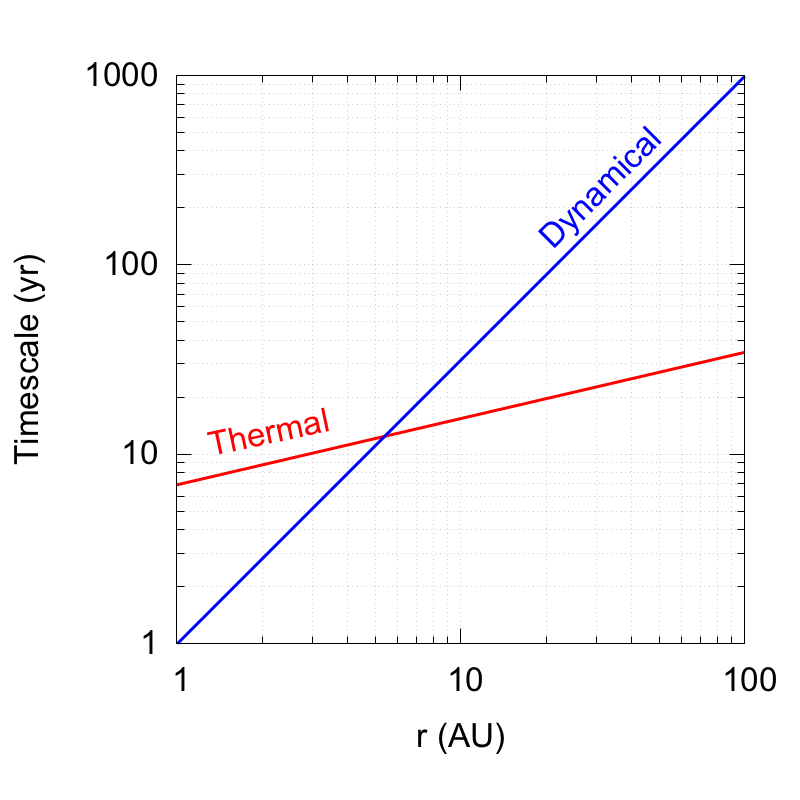
Figure 3: Thermal $t_{th}$ and dynamical $t_{dy}$ timescales vs. radius in the unperturbed disk model described in Section 2.1.

Figure 3 shows the ratio of thermal to dynamical time for the unperturbed disk model described in Section 2.1. The two time scales reach the same value of about 13 yr at $r\simeq 5.5$ AU. We call these the crossover time scale $t_{cr}$ and radius $r_{cr}$, respectively. At $r\ll r_{cr}$, where $t_{dy}\ll t_{th}$, the disk can expand or contract in the vertical direction faster than its temperature can change. Thus after each change in the illumination, the disk will gradually approach thermal equilibrium while remaining close to hydrostatic equilibrium throughout. In the opposite extreme, at $r\gg r_{cr}$ where $t_{dy}\gg t_{th}$, the vertical structure varies slower than the temperature, so under changing illumination, the disk will quickly reach thermal equilibrium while spending some time out of hydrostatic equilibrium.

The following example illustrates these two time scales’ effects. Imagine that a planet orbiting near the crossover radius opens a gap, creating a local maximum in the gas and dust density near the gap’s inner edge. The higher dust density means more starlight is intercepted here, so the disk temperature begins increasing. Since the dynamics are quicker than the heating, the disk promptly expands to the hydrostatic equilibrium corresponding to the rising temperature. As its height increases, the gap’s inner edge casts a taller shadow on the disk beyond. Under the decreased illumination, the outer regions (i.e. the regions outside the crossover radius) quickly cool off. The shadowed parts contract toward the midplane on the local dynamical time scale, which is longer than the local thermal timescale, so even after the gap’s inner edge reaches thermal and hydrostatic equilibrium, the outer disk is still contracting towards the thinner state appropriate for its new cooler temperature.

To track the disk’s response to the starlight across both regimes — with the thermal time scale the slower of the two, and with the dynamical time scale the limiting factor — we implement a sort of poor man’s radiation hydrodynamics. First, we bring the 2-D vertically-averaged hydrodynamics calculation with embedded planet to an approximate steady-state, and construct an initial guess at the 3-D density structure using the scale height $h^{0}(r)$ from the same radius in the unperturbed disk (Equation 5). Second, we send starlight into this structure using Monte Carlo radiative transfer, to determine new temperatures. Third, we adjust the structure of each patch of disk towards vertical hydrostatic equilibrium, letting the scale height change no more than permitted by the ratio of the time step to the local limiting time scale. Then we continue stepping forward in time. With each time step we compute first the new temperatures by Monte Carlo transfer, and then the new densities by letting the gas expand or contract towards hydrostatic balance. This simplified dynamics lets us determine whether the outer disk settles into a solution where it is (1) starlit, warm, and flared, or (2) shadowed, cold, and flat (Dullemond & Dominik, 2004). The final solution is both in radiative balance with the starlight, and in vertical hydrostatic equilibrium. Note that the disk can reach such a joint equilibrium only if every patch is illuminated steadily for longer than both its dynamical and thermal timescales. Faster-varying lighting, for example due to shadows cast by non-axisymmetric structures orbiting nearer the star, can maintain permanent disequilibrium, but this is not captured here.

For the radiative transfer piece of each time step, we use the Monte Carlo code RADMC-3D. This follows the paths of large numbers of photons as they are absorbed and scattered by the dust. The code is set up as spelled out in appendix B. Heating and cooling are calculated by adopting absorption and scattering opacities for spherical grains made of a mixture of astronomical silicates and carbonaceous materials, with relative abundances as in Pollack et al. (1994). The materials’ optical properties are mixed together using the Bruggeman theory to calculate the opacities for grains of a single size, which are then averaged over the size distribution $n(a)\propto a^{-3.5}$, with $a$ ranging from 0.01 to 1000 $\mu$m. Anisotropic scattering is treated using the Henyey-Greenstein phase function. The absorption and scattering opacities, and asymmetry parameter $g$, are calculated using the Mie theory and are shown in Figure 4. We have varied the dust composition and the grain size limits, with little effect on the disk’s final temperature structure.

For the gas dynamics piece of the time step, we evolve the density profile of each disk patch toward vertical hydrostatic equilibrium. We integrate the force balance equation from the midplane upwards, but let the density scale height at each point change by a fraction no greater than the time step divided by either the thermal or dynamical timescale, whichever limits the gas movements. The new density profile is closer to, but not necessarily in, hydrostatic equilibrium. To conserve mass, we adjust the midplane density at the start of the integration till the new structure has the same surface density as the old. The method is spelled out in full in appendix C.

Compared with Bitsch & Kley (2011) and Flock et al. (2013), we thus treat the gas flows in a highly simplified fashion, while giving the radiation field the comprehensive Monte Carlo transfer treatment. The method yields three kinds of model disks which we examine below: (1) in radiative equilibrium with the starlight, and in vertical hydrostatic balance, but unperturbed and planet-free, (2) disturbed by an embedded planet, and placed in radiative equilibrium with the starlight, but having the same scale heights $h^{0}(r)$ as the unperturbed model, so that it is hydrostatically out of balance, and (3) with the embedded planet, and placed in joint radiative and hydrostatic equilibrium using the poor man’s radiation hydrodynamics approach. We refer to these as models RH, P20R, and P20RH, respectively, when the planet has 20 M_⊕. Thus our complete procedure yields a total of seven models. The other four are P100R, P100RH, P1000R, and P1000RH.

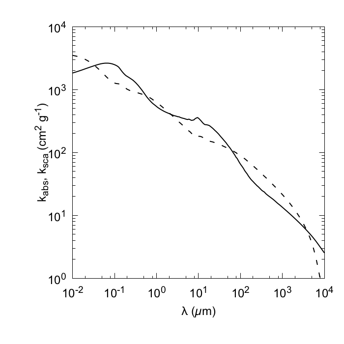
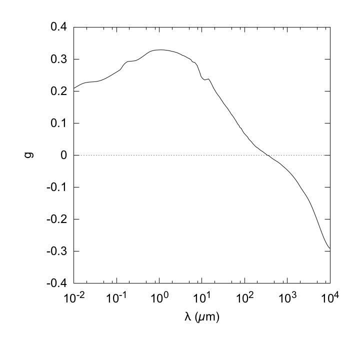
Figure 4: Left: Wavelength-dependent absorption (solid) and scattering (dashed) opacities adopted in calculating the disk’s temperature and appearance. Right: Wavelength-dependent scattering asymmetry parameter $g$.

3 Results

3.1 Planet Perturbations’ Effects on Disk Temperatures

Figure 5 shows the midplane temperature distributions in the P20, P100 and P1000 models. The top row has the radiative equilibrium models, where we neglect the planets’ effects on the pressure scale height (cases P20R, P100R and P1000R). The bottom row has the models in both radiative and hydrostatic balance (P20RH, P100RH and P1000RH). To highlight the perturbations, we plot the ratio of perturbed to unperturbed temperature, the latter being as in Equation 2. Figure 6 shows the azimuthally averaged profiles of the temperature and surface density, ratioed with the unperturbed models.

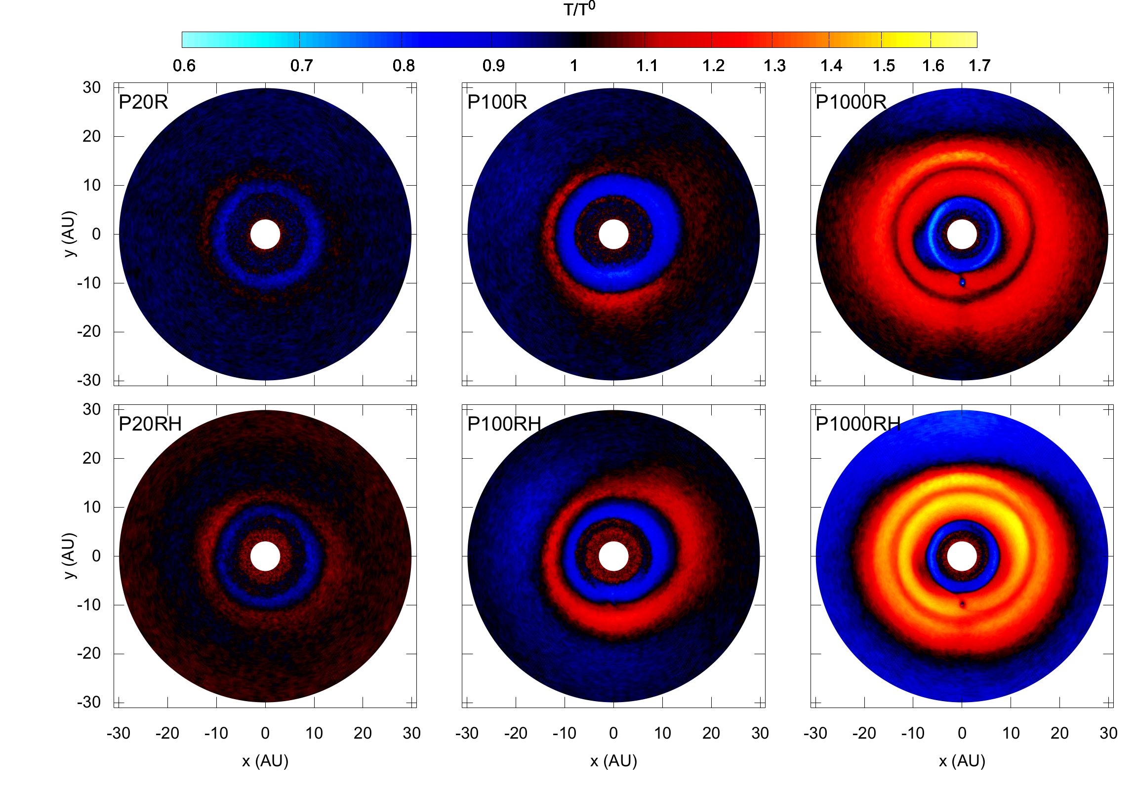
Figure 5: Midplane temperature perturbations in the models with planets of 20 (left), 100 (center), and 1000 M_⊕ (right). The top row shows models P20R, P100R and P1000R with the pressure scale height unchanged from the planet-free disk. The bottom row shows models P20RH, P100RH and P1000RH with pressure scale heights found by placing the disk in hydrostatic as well as radiative equilibrium.

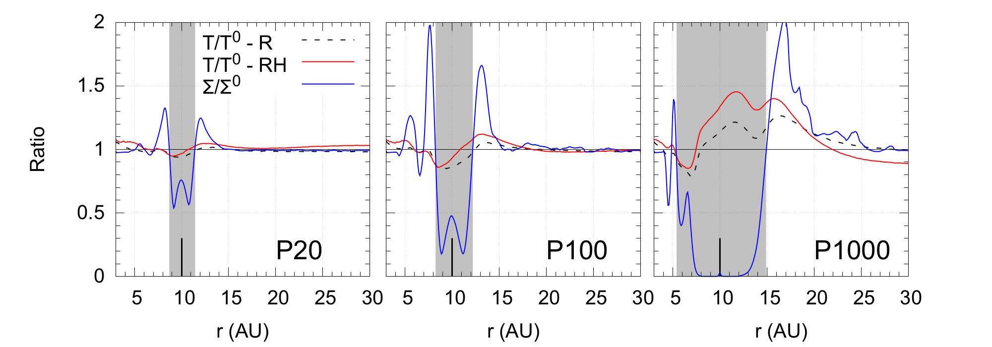
Figure 6: Azimuthally-averaged surface density and midplane temperature profiles in the 20-, 100-, and 1000-M_⊕ cases (left to right), divided by the planet-free model RH profiles. Dashed lines show models P20R, P100R and P1000R with the unperturbed scale heights, and solid lines are models P20RH, P100RH and P1000RH in hydrostatic as well as radiative equilibrium. Gray shading marks the gap opened by the planet, where surface densities are less than in the planet-free case.

The biggest disturbance in the temperature comes from the annular gap in the disk. Stronger temperature excursions generally go with stronger density perturbations, that is, with more massive planets. Among the $h=h^{0}$ cases, the temperature departs about $\pm$5% in the P20R model, and up to $\pm 30\%$ in the P1000R model. The gap is cooler by about 5% and 15% in the P20R and P100R models, respectively, while temperatures near the gap edges increase by similar fractions. In the P1000R model, temperatures both inside the gap and at its outer edge increase around 25%, while the gap’s inner edge cools by about 15%.

The disks that are also in hydrostatic equilibrium have larger temperature excursions. What’s more, the midplane temperature gradients near the planets change, such that the temperature is constant at 40 K across the gap in P20RH, while it increases with radius in P100RH and P1000RH. Specifically, the temperature rises from 37 K at 9 AU to 41 K at 13 AU in P100RH, and from 42 K at 7 AU to 56 K at 11 AU in P1000RH. In the P20RH and P100RH models, the midplane within the gap is respectively about 5% and 15% colder than the same location in the unperturbed case, while in the P1000RH model, the gap is about 40% hotter than the unperturbed disk. This difference is due to the fact that the gaps in the P20RH and P100RH models are optically thick to the starlight, while the gap is optically thin in the P1000RH model, letting more scattered starlight and thermal re-emission reach the midplane. The temperature variations in the P1000RH model are consistent with the results for Jupiter presented in Turner et al. (2012).

The outer edge of the gap opened by the planet is always hotter in the radiative-hydrostatic equilibrium models P20RH, P100RH and P1000RH than in the corresponding $h=h^{0}$ cases, and hotter than the same location in the unperturbed model. The higher temperatures mean the gap outer edges puff up and cast shadows, cooling the disk beyond. In the P20RH and P100RH models, the shadows extend to 20 and 30 AU, respectively, where the decrease in stellar gravity with distance allows the disk thickness to increase to the point where the upper layers are once again in starlight. In the P1000RH model, the shadow extends beyond 50 AU where our model ends. In this latter case, the shadowed regions’ weaker stellar illumination means temperatures are only about 90% of the unperturbed values, reducing the bolometric cooling rates roughly by half.

Finally, the temperature variations are slightly asymmetric, correlating to first approximation with the asymmetries in the surface density. For example, in the P1000RH model, the outer edge of the gap opened by the planet is hotter near the position of the density enhancement located at about 12 o’clock in figure 5 lower right panel. Along this same direction we register steeper temperature gradients between the hot gap edge and the cold outer shadowed region.

3.2 Planet Perturbations’ Effects on Panchromatic Disk Continuum Emission

We construct synthetic images of all seven models using the ray-tracing module of RADMC3D, at wavelengths of 1 $\mu$m, 1 mm, and 1 cm. Whereas the near-infrared is dominated by stellar radiation scattered by sub-micron grains located in the disk’s surface layers, the emission at millimeter and centimeter wavelengths is mostly thermal, and originates from larger particles near the midplane. For simplicity, we generate synthetic images with the disk face-on. Furthermore, to better show the planet’s effects on the disk’s appearance, in all following figures we ratio each image with that of the unperturbed model RH.

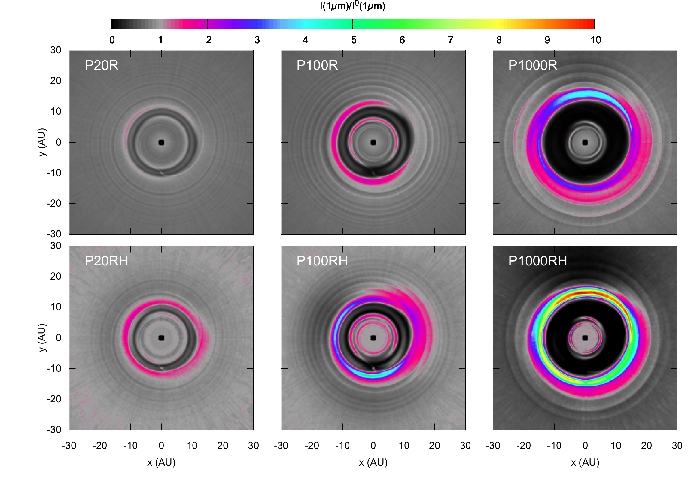
Figure 7: Maps of the 1 $\mu$m scattered light for the 20 (left), 100 (middle), and 1000-M_⊕ cases (right) viewed face-on. The top row shows the models in radiative but not hydrostatic equilibrium, P20R, P100R and P1000R. The bottom row has the corresponding models in both radiative and hydrostatic balance, P20RH, P100RH and P1000RH.

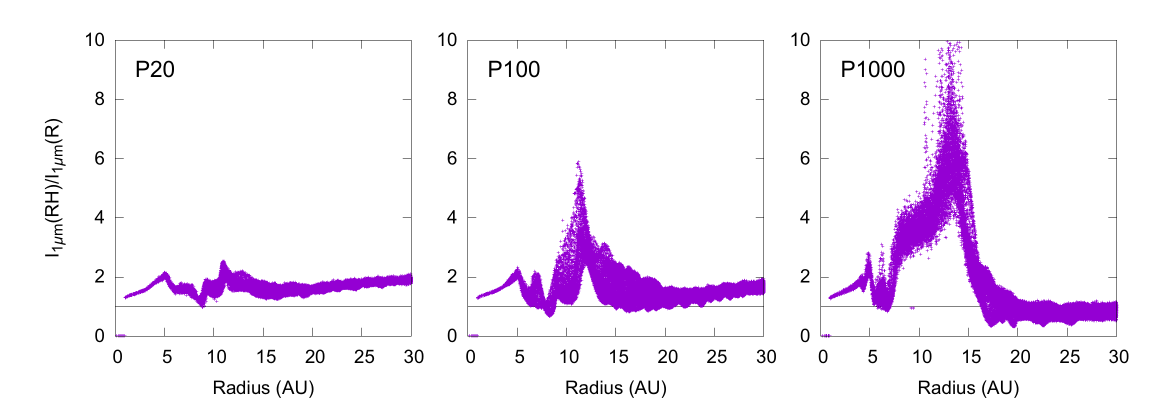
Figure 8: Ratio of the scattered light at 1 $\mu$m between the models in joint radiative and hydrostatic equilibrium (RH, shown in the bottom panels of Figure 7) and those in radiative but not hydrostatic equilibrium (R, shown in the top panels of Figure 7). Each point represents one pair of corresponding pixels.

The 1 $\mu$m synthetic images appear in Figure 7. Their strongest features are dark and bright rings tracing, respectively, the gap opened by the planet and its outer edge. The hydrostatic equilibrium models also have a broad dark ring where the gap’s puffed-up outer edge throws its shadow. The intensity of the bright ring at the gap’s outer edge depends sensitively on the disk’s vertical structure (Figure 8): its surface brightness is 1.5-4 times the planet-free case in the three R models which are out of hydrostatic balance, and 3-10 times the planet-free case in the three RH models, where hydrostatic balance is restored. In this and other ways, the R- and RH-models appear quite different, despite having identical surface density maps.

In the hydrostatic models, the region shadowed by the gap’s outer edge scatters starlight with surface brightness just a fraction of the same locations in the unperturbed disk. In contrast, the $h=h^{0}$ R-models show no such shadowing. Because of its sensitivity to the scale height, the scattered light is a poor tracer of the surface density. Relating scattered light features directly to density variations can lead to serious errors.

Another notable feature of the scattered light images is that the planets’ outer spiral density waves are brighter in the radiative equilibrium R-models than in the radiative-hydrostatic equilibrium RH-models. For example, in the P1000R model, the spiral arms near 20 AU are 1.5 to 2 times brighter than surrounding regions, a contrast similar to the amplitude of the spiral density wave. However in the corresponding hydrostatic P1000RH model, the spiral arms disappear in the dark ring beyond the gap’s outer edge. We will come back to this point in Section 5 in comparing models to observations.

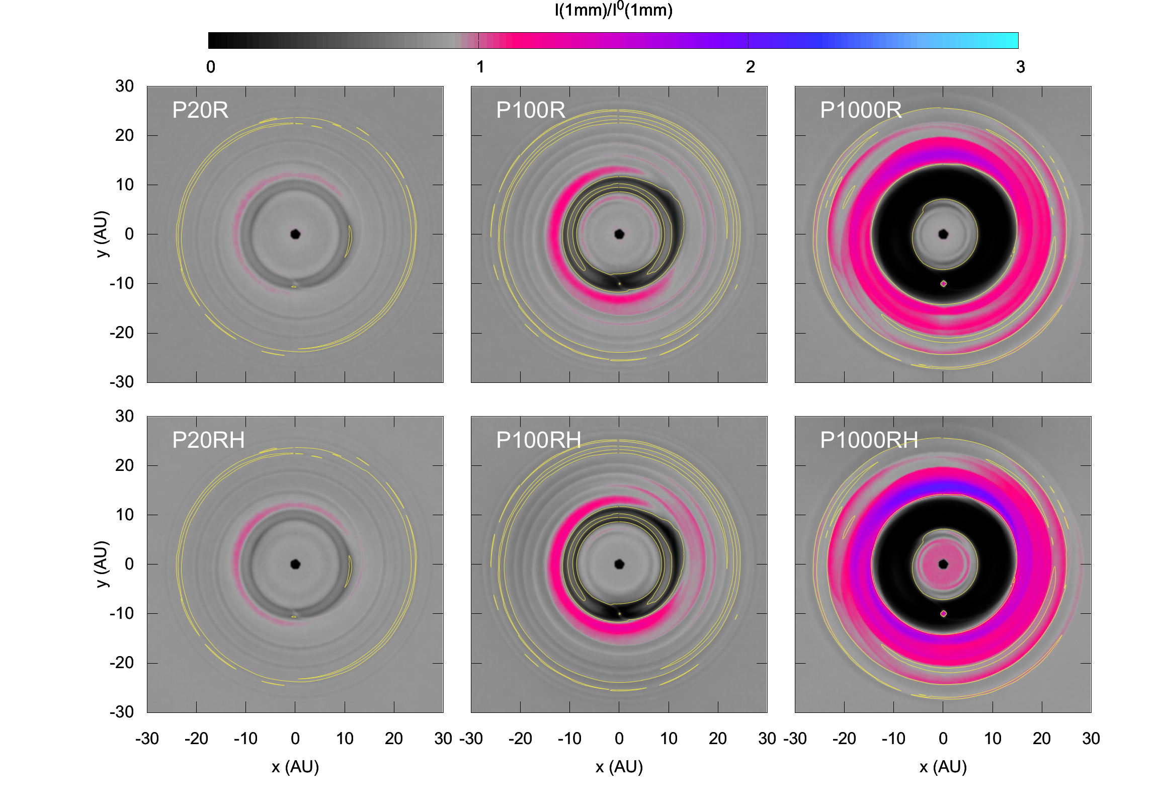
Figure 9: Maps of the 1 mm continuum emission from cases with planets of 20 (left), 100 (middle), and 1000 M_⊕ (right) viewed face-on. The top row shows the radiative equilibrium models P20R, P100R and P1000R. The bottom row has the radiative-hydrostatic models P20RH, P100RH and P1000RH. Yellow contours mark monochromatic optical depth unity.

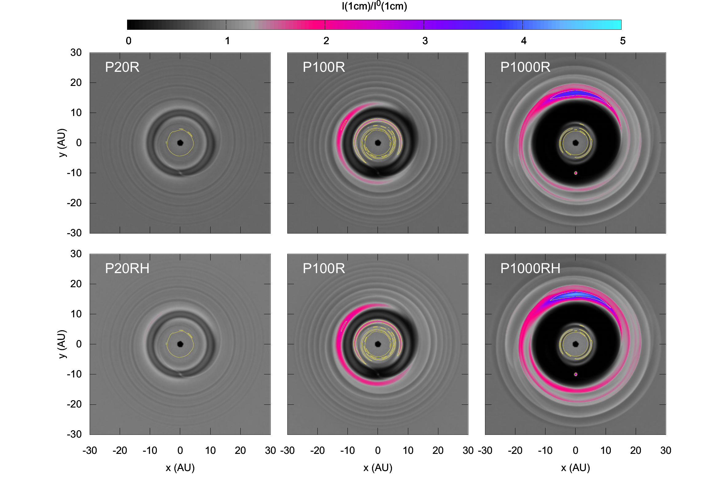
Figure 10: As Figure 9 but for the wavelength of 1 cm.

Figures 9 and 10 show the ratio between the dust emission of the perturbed and unperturbed disk models at wavelengths 1 mm and 1 cm, respectively. As in the scattered light, the gaps opened by the planets appear as dark annuli, and the gaps’ outer rims appear as bright annuli. Azimuthal asymmetries due to vortices orbiting near the gaps’ outer edges are also visible.

For our assumed dust opacity and initial surface density, the 1 mm emission arising within 20 AU of the central star is mostly optically thick, and so probes spatial variations of the temperature rather than the surface density. For example, in the P20 models, the dark ring at the partially depleted, but still optically thick, gap comes from the low temperature in the gap discussed in Section 3.1 and is not due to the lower surface density. The large optical depth also reduces the visibility of the azimuthal asymmetries in the P100 and P1000 models. In both the P1000R and RH models, the intensity ratio at the center of the vortex on the gap’s outer edge is about 2.5, which is only about half the surface density ratio (Figure 1).

Since the 1 mm emission probes temperatures, it indirectly informs us about the vertical structure of the disk. In particular, the radiative-hydrostatic equilibrium RH-models have brighter gap outer edges, and fainter shadowed regions, than the radiative-equilibrium-only R-models. The starlight illumination is thus important for interpreting millimeter-wave observations of the optically-thick parts of protostellar disks.

The dust thermal emission at the wavelength of 1 cm from regions more than 5 AU from the star is mostly optically thin. It more closely probes the surface density perturbations caused by the planets. For example, at the gap’s outer edge the intensity varies with azimuth by factors of about 1.3 in the P20RH model, and about 5 in the P1000RH model, similar to the azimuthal ranges in the surface density shown in Figure 1. As with the 1 mm emission, the radiative equilibrium and radiative-hydrostatic equilibrium models look different at 1 cm wavelength, following the corresponding variations in the dust temperature discussed in the previous section.

4 Consequences for Gas and Planet Dynamics

The main goal of our investigation is to understand young planets’ effects on the multi-wavelength dust continuum emission from protostellar disks, especially at the locations outside 5 AU where starlight dominates the heating. In pursuing this, we have found that the planet-disk interaction produces more than the long-predicted surface density perturbations: it also significantly perturbs temperatures across the disk. In this section, we elaborate on the temperature perturbations’ consequences for the dynamics of gas, dust and planets.

4.1 Heating and Cooling

We showed in Section 3.1 that perturbing planets of more than about 20 $M_{\oplus}$ yield variations in the disk temperature with respect to a planet-free disk. This means that evolving the disk with an isothermal equation of state produces errors, and that reliable hydrodynamical modeling requires treating the heating and cooling. The need for something beyond a simple power-law relationship between temperature and density is illustrated in Figure 11, a map of the index $\gamma-1$ in the relationship $T(r,\phi)\propto\rho^{\gamma-1}(r,\phi)$ applied to the disk’s evolution from the unperturbed state to the planet perturbation in radiative-hydrostatic equilibrium. The index is calculated by

$$\gamma-1=\log(T_{m}^{RH}/T_{m}^{0})/\log(\rho_{m}^{RH}/\rho_{m}^{0}),$$ (14)

where $T_{m}^{0}$ is the midplane temperature of the unperturbed disk and $T_{m}^{RH}$ is the midplane temperature in the RH-model. Isothermal evolution corresponds to $\gamma-1=0$, and adiabatic evolution of molecular hydrogen corresponds to $\gamma-1=0.4$. Clearly the evolution from the unperturbed to planet-perturbed models is not well described by a single value of $\gamma$. Note that $\gamma-1$ is near zero within the gap opened by the planet not because the temperature is time-constant, but because the change in density is so much greater than the change in temperature. Generally, $\gamma-1$ ranges from positive to negative values as we move from patches of the disk directly lit by the star to those lying in the shadows.

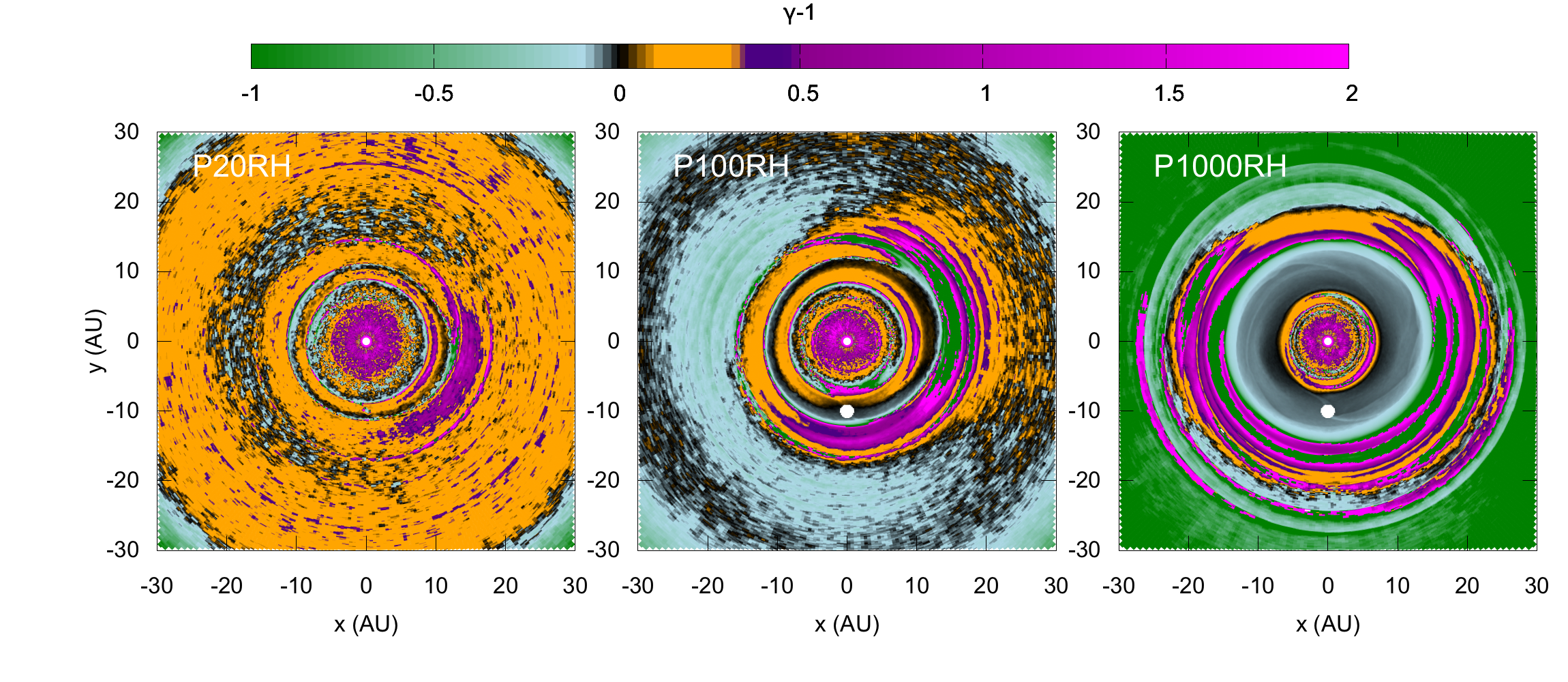
Figure 11: Maps of the power-law index in $T\propto\rho^{\gamma-1}$ describing the pointwise change in midplane temperature and density between the disk’s unperturbed state and its radiative-hydrostatic equilibrium with an embedded planet. The three panels show models P20RH, P100RH and P1000RH (left to right).

Another consequence of the changes in surface density and temperature across the disk is new values for the thermal time scale discussed in section 2.4. In figure 12 we show the ratio of the thermal to the dynamical time scale in the three radiative-hydrostatic equilibrium cases. The 20-M_⊕ model is broadly similar to the unperturbed profile in figure 3. The 100-M_⊕ model cools faster in the gap owing to the lower surface density, and cools slower in the outer shadowed region owing to the low temperatures. The 1000-M_⊕ model is a more extreme version of the 100-M_⊕ case, with shadows so deep and cold that temperatures change only over time scales comparable to or longer than the local orbital period. Apparently gap-opening planets can drastically change the surrounding disk’s thermal timescale, and thus its response to changing illumination.

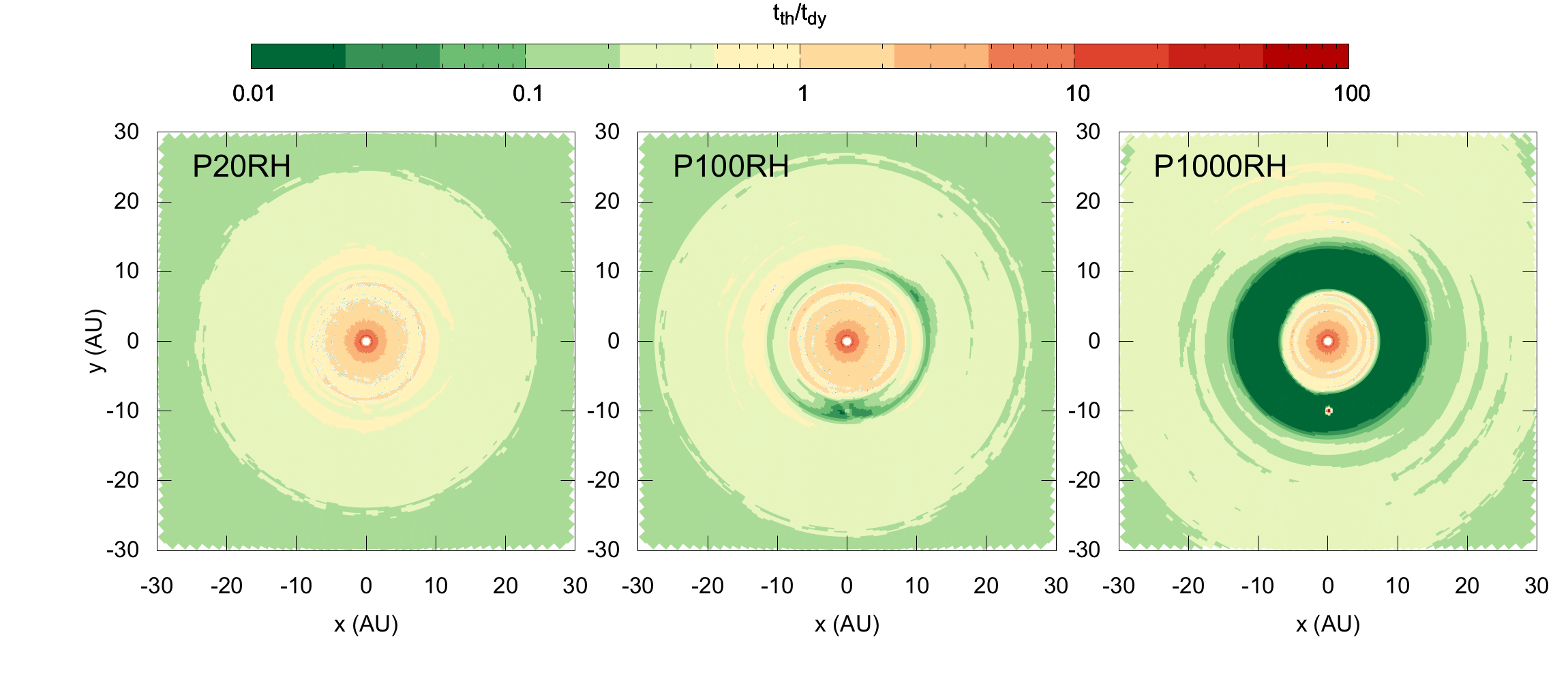
Figure 12: Ratio between the thermal and dynamical time scales. The three radiative-hydrostatic equilibrium models P20RH, P100RH and P1000RH appear from left to right.

4.2 Orbital Migration

Temperature perturbations caused by the planet-disk interaction might also affect the planet’s long-term orbital migration, which is governed by the gravitational forces exchanging angular momentum between planet and disk. If $M_{p}\ll M_{th}$, the rate and direction of migration are sensitive to the disk’s temperature and density structure. In a power-law model disk defined by $T\propto r^{-\beta}$ and $\Sigma\propto r^{-s}$, with $\beta$ between 0.1 and 0.5, and $s$ between 1 and 1.5, an Earth-mass planet migrates inward at a rate as high as $10^{-5}$ AU/yr (Ward, 1997; Papaloizou & Terquem, 2006). However, sufficiently steep radial temperature gradients can slow and even reverse the motion. In particular, outward migration is expected within a few AU of the star, where accretion is the main source of heating, while inward migration should occur at larger radii (Paardekooper & Mellema, 2006; Lyra et al., 2010; Paardekooper et al., 2011; Bitsch & Kley, 2011). Our results suggest that planets less than $M_{th}$ perturb the temperatures too little to affect the migration rate. However, low-mass planets could find themselves migrating along the temperature gradients arising from a more massive companion’s interaction with their shared host disk.

Temperature perturbations’ effects on planets with $M_{p}\sim M_{th}$ have received too little attention. Jang-Condell & Sasselov (2005) found that the density and temperature perturbations near Neptune-mass planets can substantially slow their inward migration. Similar results were found by D’Angelo et al. (2003), who moreover argued that the lack of an appropriate energy equation is the main limitation in modeling such planets’ dynamics. Our results show that planets with close to the thermal mass (as in the P20 models) produce disturbances of about $\pm$10% in the gas temperature (Figure 6). More importantly, in the P20RH model, the temperature gradient within the planet’s partially depleted gap is close to zero. Quantifying the effects such perturbations have on the migration requires numerically integrating the torque exerted by the disk on the planet, which is beyond the scope of this work. Instead, we seek a qualitative understanding of the effects on low-mass planets’ migration by assuming the total torque $\Gamma_{tot}$ is the sum of the Lindblad torque $\Gamma_{L}$ and the horseshoe corotation torque $\Gamma_{hs}$ expressed as (Paardekooper et al., 2011; Bitsch et al., 2013; Baruteau et al., 2014)

$$\Gamma_{tot} = \Gamma_{L}+\Gamma_{hs},$$ (15)

$$\gamma\frac{\Gamma_{L}}{\Gamma_{0}} = -2.5-1.7\beta+0.1s,$$ (16)

$$\gamma\frac{\Gamma_{hs}}{\Gamma_{0}} = \frac{7.9}{\gamma}(\beta-(\gamma-1.0))s,$$ (17)

$$\Gamma_{0} = \left(\frac{q}{h}\right)^{2}\Sigma_{p}r_{p}^{6}\Omega_{p}^{2},$$ (18)

where $\gamma$ is the effective ratio of specific heats for the disturbances the planet launches, taking into account radiative diffusion. If the disturbances are so optically thick they trap their thermal radiation, then they propagate through the disk in the adiabatic limit, with $\gamma=1.4$ for molecular hydrogen gas. If the photons quickly smooth out temperature variations, then the disturbances propagate isothermally, and $\gamma=1$. In the models we consider, the thermal timescale at the planet is about half the orbital period, so the thermal diffusivity is $2h^{2}\Omega/(2\pi)$. The effective equation of state considering disturbances of all wavenumbers is then around $\gamma=1.2$, judging from the numerical results shown in figure 8 of Paardekooper et al. (2011). This implies that the total torque in the unperturbed model ($s=1$, $\beta=0.45$) is negative with $\Gamma_{tot}/\Gamma_{0}=-1.3$, indicating inward migration as expected. In model P20RH, the surface density near the planet’s orbit also varies as $r^{-1}$, while the temperature is roughly constant between 9 AU and 11 AU, an annulus that spans both the horseshoe region and the Lindblad resonances’ pileups inside and outside the planet’s orbit, and thus most strongly affects the planet. The uniform temperature yields a more negative torque $\Gamma_{tot}/\Gamma_{0}=-3.1$, indicating faster inward migration.

Finally, planets much more massive than $M_{th}$ clear gaps, and so are thought to migrate following the global inflow of the circumstellar gas. The massive planets through their temperature perturbations might not affect their own migration rate, but they can alter the migration of nearby low-mass planets. For example, the P1000RH model in figure 5 at 15-20 AU, in the shadow of the gap’s outer edge, has midplane temperature scaling as $T\propto r^{-1.6}$. Across the same annulus, the surface density varies as $\Sigma\propto r^{-3.9}$. Equations 15-17 above indicate that a low-mass planet ($M_{p}\ll M_{th}$) orbiting here feels a positive torque ($\Gamma_{tot}/\Gamma_{0}\sim 26$) so migrates rapidly outward. Positive torques also occur in the shadowed regions of the P20RH and P100RH models. Further out in each shadow, the temperature and surface density gradients flatten, and the torque turns negative. Migrating low-mass planets thus likely converge within the shadows cast by the gaps opened by the massive planets.

5 Consequences For Interpreting Features in Protostellar Disks

5.1 Taxonomy

This section is devoted to the models’ implications for interpreting recent observations. Many protostellar disks feature annuli, crescents, and circular and spiral arcs in the dust and gas emission, as revealed through the improved sub-arcsecond mapping capabilities of infrared cameras such as HiCIAO/Subaru, Sphere/VLT, GPI/Gemini, and millimeter and centimeter arrays including CARMA, SMA, ALMA and the VLA. A list of such disks is in Table 1. Whether these structures, and their diversity, result from the interaction between the circumstellar material and forming planets, or are caused by other processes, is debated.

The SAO 206462 and J160421.7-213028 systems are good examples of the diverse morphologies observed in protostellar disks (Figure 13). At sub-millimeter wavelengths, both disks show partially depleted dust cavities tens of AU in diameter (Pérez et al., 2014; Zhang et al., 2014; van der Marel et al., 2016; Dong et al., 2017). However, while the dust continuum in the SAO 206462 disk traces a ring and a crescent, the J1604 disk appears almost axisymmetric. At near-infrared wavelengths, the SAO 206462 disk exhibits an $m=2$ grand design spiral, while the J1604 disk appears as a circularly symmetric annulus.

The crescents observed in the microwave regime come with a large spread of amplitudes, defined as the difference between the maximum and minimum flux densities measured at the same orbital radius divided by the minimum intensity, $a=(F_{max}(r)-F_{min}(r))/F_{min}(r)$. IRS 48 has the most prominent crescent observed so far, with an amplitude greater than $100$; MWC 758, SAO 206462, LkHa 330 and SR 21 have much more moderate amplitudes between 1.5 and 3. Recent data show that crescents at sub-millimeter wavelengths are accompanied in most cases by near-infrared spiral features. This is the case for AB Aur, MWC 758, SAO 206462 and HD 142527.

The observations collected so far reveal a second trend: the earlier the spectral type of the star, the more complex the morphology of its disk. For example, the disks around HD 100546 and AB Aur, which have spectral types of B9.5 and A0, respectively, show multiple spiral features in the near-IR. The AB Aur disk has a complex morphology also at millimeter wavelengths, showing a crescent and spiral features in the molecular line emission (Tang et al., 2012). The disks around MWC 758, SAO 206462, and HD 142527, with spectral types between A5 and F7, have $m=1$ or $m=2$ spiral structures. The disks around HD 97048 (A0), HD163296 (A1), HD 169142 (A5) are exceptions in that they do not show spiral features. In contrast, the disks around late G, K and M stars are mostly characterized by azimuthally symmetric rings at both infrared and millimeter wavelengths.

Finally, we note that in classifying perturbed disks, we explicitly avoid making use of the morphology of the molecular line emission observed with ALMA. The main reason is that spatially-resolved maps of the molecular line emission are available only for a few of the disks listed in Table 1. The molecular line emission however provides valuable information on the nature of the structures observed in disks. For example, ALMA observations of HD 142527, SAO 206462, and MWC 758 show that the ¹³CO and C¹⁸O are distributed much more nearly axisymmetrically than the dust. This suggests the crescent observed in the millimeter-wave continuum could result from the decoupling of large dust grains from the gas.

Table 1: Protostellar disks around stars not known to be double or multiple, and which show small-scale morphological features. The list includes only objects with high-quality imaging at both near-infrared (NIR) and millimeter wavelengths (mm). The source list is ordered by stellar spectral type. In Columns 4 and 5, we report the main morphological feature characterizing NIR and mm observations, respectively. The parameter $m$ indicates the number of structures. The parameter $a$ indicates the azimuthal contrast in the dust continuum emission at the crescent(s)’ orbital radius.

(1)	(2)	(3)	(4)	(5)	(6)
Name	Sp.T.	M⋆	NIR	mm	ref.
HD 100546	B9.5	2.4	Spiral, $m\geq 3$	Ring, $m\geq 1$
HD 97048	A0	2.5	Ring, $m\geq 4$	Ring , $m\geq 2$
AB Aur	A0	2.0	Spiral, $m\geq 5$	Crescent, $m\geq 1$, $a\sim 4$
IRS 48	A0	2.0	Spiral, $m\geq 1$	Crescent, $m\geq 1$, $a>100$
HD 163296	A1	2.3	Ring, $m\geq 1$	Ring, $m\geq 3$
MWC 758	A5	2.0	Spiral, $m\geq 2$	Crescent, $m\geq 2$, $a\sim 1.5,3$
HD 169142	A5	2.0	Ring, $m\geq 2$	Ring, $m\geq 2$
SAO 206462	F4	1.7	Spiral, $m\geq 2$	Ring, $m\geq 1$; Crescent, $m\geq 1,a\sim 3$
LkH$\alpha$ 330	G3	2.5	Spiral, $m\geq 1$	Crescent, $m\geq 1,a\sim 1.5$
SR 21	G3	2.5	No structures	Crescent, $a\sim 3$
J160421.7-213028	K2	1.0	Ring, $m\geq 1$	Ring, $m\geq 1$
LkCa 15	K3	1.0	Ring, $m\geq 2$	Ring, $m\geq 1$
RX J1615-3255	K5	1.1	Ring, $m\geq 3$	Ring, $m\geq 1$
PDS 70	K5	0.8	Ring, $m\geq 1$	Crescent, $a\sim 1.5$
TW Hya	K6	0.8	Ring, $m\geq 5$	Ring, $m\geq 6$

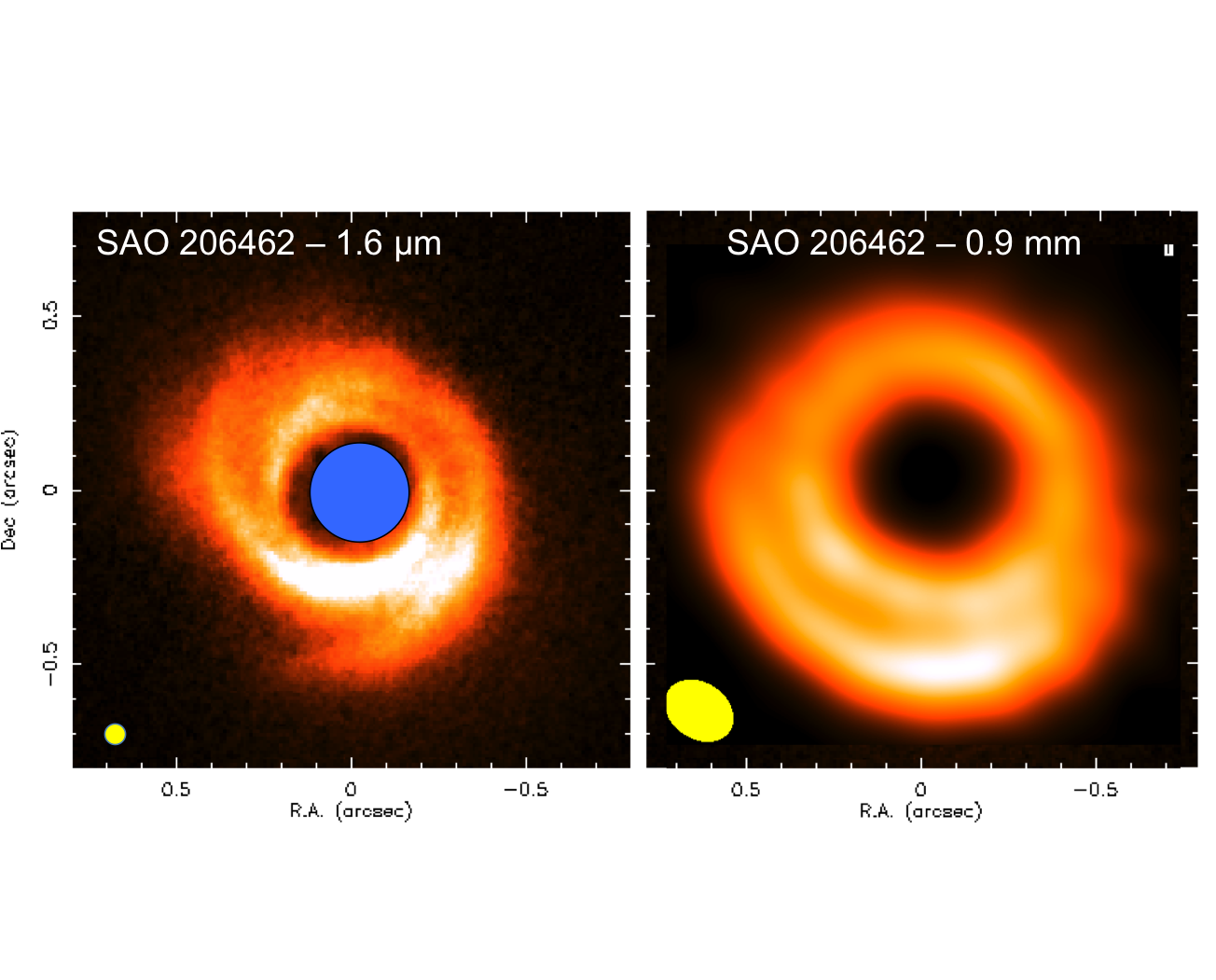
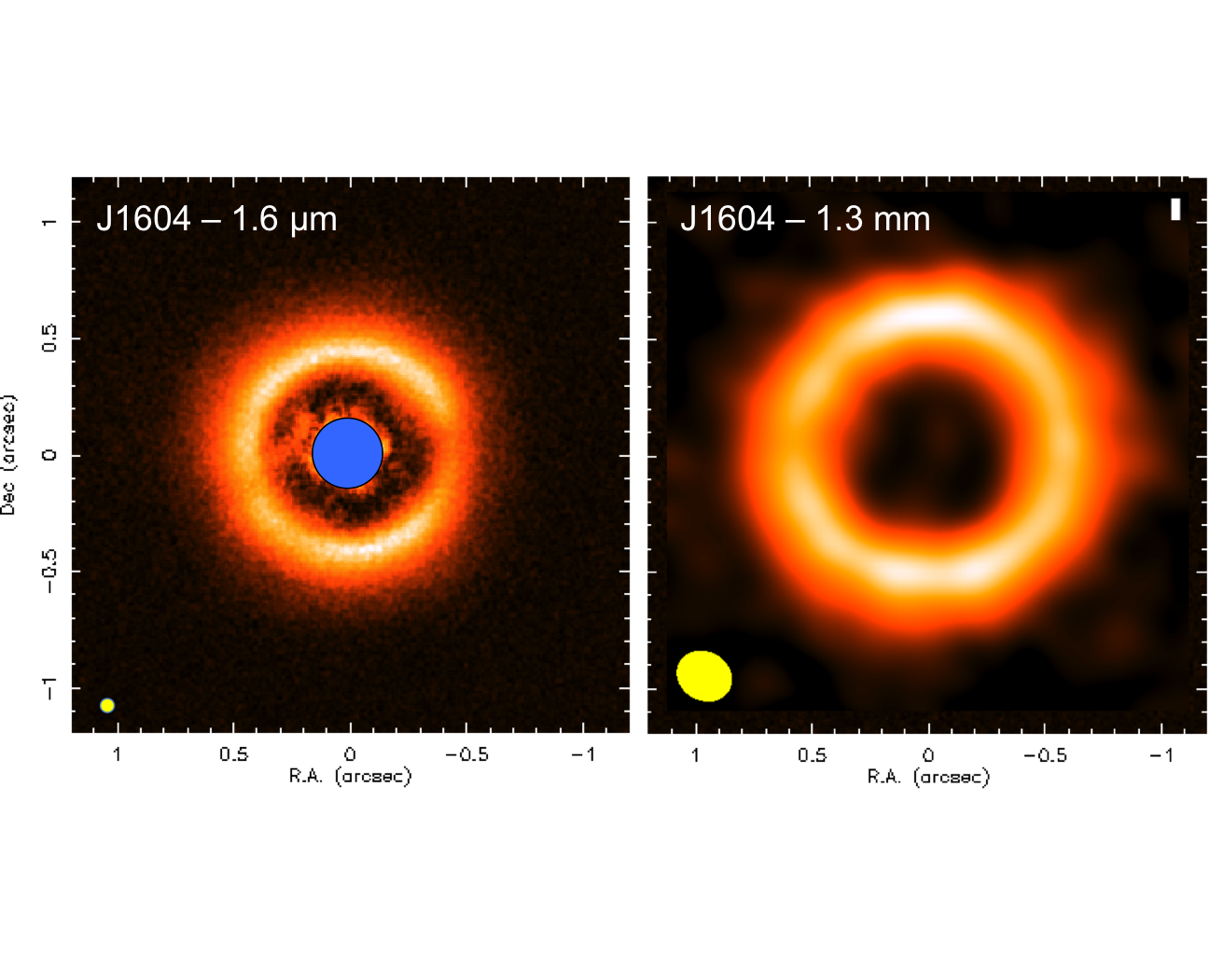
Figure 13: Maps of the SAO 206462 (top) and J1604 (bottom) disks recorded in the continuum emission at 1.6 $\mu$m (left) and $\sim$1 mm (right). These maps illustrate the diversity of structures observed in protostellar disks, which include spiral and circular arcs, as well as crescents. The observations are taken from Muto et al. (2012), Mayama et al. (2012b), Dong et al. (2017) and van der Marel et al. (2016).

5.2 Comparing Models With Observations

Annuli: The models discussed in Section 3.2 show that the disk-planet interaction can naturally lead to ring-like structures in both the infrared scattered light and millimeter-wave emission, similar to those observed toward dynamically-cold disks. For example, the annular emission observed toward J160421.7-213028 is very similar to the synthetic maps for the P1000 model shown in the bottom-right panels of Figure 7 and 9. In both the model and the observations, the scattered light emission is confined to a narrow ring, whereas dust is present on a much wider area (Zhang et al., 2014; Dong et al., 2017). In the case of HD 169142, polarimetric images obtained at about 0.7 $\mu$m show a narrow bright ring with a radius of 23 AU, surrounded by a wide dark annulus extending to about 65 AU and a second wide bright ring extending outward of 65 AU (Bertrang et al., 2018). These structures are also very similar to those observed in our models, where the dark ring might trace the shadow cast by the outer rim of the gap created by a planet. In our model, rings seen in scattered light are narrow because scattered light arises from the puffed-up outer edge of the gap opened by the planet. If, instead, the disk vertical structure were unaffected by the planet, scattered light would come from a wider annulus as shown in the top-right panel of Figure 7. Clearly the vertical structure is a key factor in interpreting scattered light maps of protostellar disks.

The effect of the vertical structure on the scattered light emission can be understood by analogy with a mountain illuminated by the Sun at sunset, as seen by an observer flying over it. Only the part of the mountain facing west will be illuminated, while its east side and the surrounding valleys will be in the dark. The shape of the illuminated side will depend on the shadows cast by the terrain westward of the mountain, but, in general, the higher the mountain, the larger the fraction lit by the setting Sun. The outer edge of the gap opened by the planet is similar to such a mountain. Indeed, this region is hotter, and therefore more puffed-up, than the surrounding area because it is directly illuminated by the star (Section 3.1).

Crescents: In an inviscid or low viscosity disk, the disk-planet interaction produces vortices near the outer rim of the gap opened by the planet. This could naturally lead to the crescents observed in the millimeter- and centimeter-wave dust continuum emission, if the vortices concentrate sub-millimeter and millimeter-sized particles through gas drag forces. The strongest concentrations toward gas pressure maxima are expected to occur for particles whose aerodynamic stopping time is comparable to the orbital period, so that the Stokes number $St\sim 1$ (Section 2.3).

The crescents observed in perturbed disks are characterized by azimuthal variations in the flux density with amplitudes between 1.5 and more than 100 (Table 1). Even if the dust emission is optically thin, and therefore traces the dust column density, measuring the amplitude of the crescent is by itself insufficient to determine the degree to which the dust has been concentrated relative to the gas. We must also measure the azimuthal variation in the gas density. Nevertheless, hydrodynamic models indicate that a single planet generates azimuthal perturbations on the gas surface density of up to a factor of a few (Figure 1). Similar values are obtained with multiple planets (e.g. Isella et al., 2013). Therefore, the large-amplitude crescents observed in HD 142527 (amplitude 30) and IRS 48 (amplitude $>100$) require dust and gas be dynamically decoupled.

The degree of separation of dust and gas can be measured by comparing maps of the optically-thin dust and trace molecular species’ emission. The latter is the best probe of the total gas mass, since the main component, molecular hydrogen, is not itself observable. In the case of the HD 142527 circumbinary disk, Boehler et al. (2017a) find that the large crescent observed in the dust emission corresponds to an azimuthal variation of a factor of 54 in the density of millimeter grains, but only a factor of about 4 in the density of ¹³CO and C¹⁸O molecules. While the conversion from CO to H₂ density is hampered by uncertainties in the molecular abundance (see, e.g., Willacy & Langer, 2000; Aikawa et al., 2002; Qi et al., 2015; Miotello et al., 2017), this result suggests that vortices concentrate dust efficiently, and that even the more prominent dust crescents might be compatible with azimuthal variations in the gas density such those predicted by planet-disk interaction models.

The disks surrounding SAO 206462 (fig. 13; van der Marel et al., 2016) and MWC 758 (Boehler et al., 2017b) show complex combinations of rings and crescents. In the first case, an azimuthally extended dust crescent is observed outside a ring, which itself shows azimuthal variations in the millimeter-wave dust emission. In the second case, the 0.87 mm dust continuum emission shows two dust crescents centered about 47 and 82 AU from the central star, and characterized by azimuthal variations in the dust emission by factors of 1.5 and 2, respectively. Qualitatively, these features resemble the structure of the P100RH and P1000RH models, where dust crescents form at both edges of the gap formed by a planet. If this model applies, the perturbing object might be located at a radius of about 65 AU in the case of MWC 758, and about 55 AU in the case of SAO 206462.

Spirals: Interpreting protostellar disks with grand design spirals in the framework of planet-disk interaction is problematic. Our models suggest the planet-generated spiral density waves have quite weak signatures at near-infrared wavelengths (Figure 7). This is because the outer edge of the gap cleared by the planet casts a shadow on the outer disk, strongly reducing the visibility of any spiral feature located outside the gap. A similar result was obtained by Juhász et al. (2015), who constructed synthetic scattered light images for a disk perturbed by planets, assuming that the disk pressure scale height scales as a power law with the radius (their Figure 2). As shown in Figure 7, the spirals’ visibility at infrared wavelengths is even worse when the pressure scale heights are consistent with hydrostatic equilibrium.

Another problem is the large pitch angles of the spiral arms observed in the near-infrared. Since the pitch angle of a spiral density wave launched by a planet increases with the gas temperature (see Section 2.2), large angles imply high temperatures. By comparing MWC 758 observations with the analytical solution of Equation 7, Benisty et al. (2015) inferred that the disk temperature at the location of the spirals should be several hundred degrees Kelvin, at least ten times greater than the temperature calculated based on the stellar flux received. How can the disk reach such high temperatures? Lyra et al. (2016) suggest the disk might be heated as the density waves launched by a massive planet (5 M_J) shock the circumstellar gas. Note that this works only if the heat is not radiated away, but remains in the disk from one shock passage to the next – that is, $t_{th}$ must exceed $t_{dy}$, which in our initial disk model happens only within 10 AU of the star.

Furthermore, the shock heating is deposited preferentially near the planet’s innermost Lindblad resonances, which lie close to the edges of the gap the planet opens in the disk (Figure 3 of Lyra et al., 2016). Hot gas at the Lindblad resonances would mean a taller outer edge for the gap, which could even reduce the visibility of spiral waves in the scattered light emission. It is also not yet clear whether such hot material would produce hot spots visible in the mid-infrared or millimeter continuum emission. ALMA observations constrain the temperatures of dust and gas (most gas measurements are of carbon monoxide) near the spiral arms to less than 40 K in agreement with predictions from stellar irradiated disk models (Muto et al., 2015; Boehler et al., 2017b).

As a solution to both the spirals’ visibility and the pitch angle problem, Dong et al. (2015b) have suggested the observed spiral waves might be excited by a massive planet ($>5$M_J) orbiting outside the cavities observed at millimeter wavelengths, and beyond the spiral features observed in the near-infrared. In this model, the observed spirals correspond to the arms propagating inward from the planet orbital radius. This is similar to the picture proposed by Muto et al. (2012) to explain the large pitch angle of the spiral features observed in the SAO 206462 disk. In the case of MWC 758, Dong et al. (2015b) calculate that the planet would have an orbital radius of about 160 AU (their Figure 4). For this model to work, the planet must be very young. In particular, the age of the planet must be less than the time required to open a gap in the disk. This is because once the gap is fully opened, the part of the spiral density wave with the largest pitch angle will be located within the dust depleted gap, making the spiral disappear at infrared wavelengths. In the specific case of MWC 758, Dong et al. (2015b) manage to reproduce the observations by halting the hydrodynamic simulation after 20 orbits of the planet, or about $0.3\times 10^{5}$ yr for an orbital radius of 160 AU. The entire gap opening phase takes $0.6\times 10^{5}$ to $1.5\times 10^{5}$ yr, depending on the accretion stress. If the observable lifetime of the spiral is so short, objects like MWC 758 and SAO 206462 should be a small fraction, probably less than 10%, of the disk population forming giant planets at large separation. This seems to conflict with the fact the spiral arcs are observed in the majority of perturbed disks around early type stars.

A third hypothesis, advanced by Dong et al. (2015a), is that the spirals observed in scattered light result from the disk’s gravitational instability. To be gravitationally unstable, disks must be massive. Dong et al. (2015a) find that the spiral structures in SAO 206462 and MWC 758 require disk masses of 0.25 and 0.5 M_⊙, respectively. These are much greater than the masses derived from observations of the millimeter-wave dust emission, which suggest instead masses of about 0.025 and 0.01 M_⊙, respectively (Isella et al., 2010; Andrews et al., 2011b).

Finally, a fourth hypothesis is that the spiral features are due to material orbiting near the star which casts shadows that appear as spirals because they sweep across the disk at the finite speed of light (Kama et al., 2016). Forming bright spiral arms this way requires notches in the screening material to let through narrow beams of starlight, while variability surveys suggest narrow-angle obscuration is more common (Cody et al., 2014; Stauffer et al., 2015).

Clues to the causes of the spiral features observed in the near-infrared might be gained by looking at the ensemble of perturbed disks listed in Table 1. For example, as noted above, five of the eight disks around A and F stars are characterized by spiral features, while no spirals are detected in the disks of the K type stars for which observations exist. Whereas we cannot exclude that this trend might be an artifact of the small sample, the available observations suggest that the formation of spiral arms somehow depends on the stellar mass.

It is worth noting that early-type stars are mostly in binary or multiple systems. The multiplicity fraction of mature G-type stars is 57%, complete down to a companion-to-primary mass ratio of 0.1. This fraction is higher among A- and F-type stars. The large fraction of multiples among the main-sequence stars suggests a correspondingly high fraction of multiples among young early-type stars. Based on this consideration, we suggest that the observed perturbations might be due to the presence of yet unseen, close separation, stellar mass companions, instead of planets. A companion with greater mass will excite stronger density waves, which might warm up the circumstellar gas through shock heating, as remarked above, or induce other kinds of instability in the disk. The heating from the companions should also be taken into account in future hydrodynamical modeling of this scenario.

A companion might be responsible for at least one of the dynamically-hot disks listed in Table 1. The star HD 142527 has a 0.25 M_⊙ companion orbiting at 10 AU. This binary system has a mass ratio of 8, much lower than those in the models we present here, which range from 330 to 16700. Searches for companions around the other dynamically-hot disks listed in Table 1 have resulted in no detections to date, but most of these observations are sensitive mostly to companions at separations larger than 10 AU (Isella et al., 2014, and references therein).

6 Conclusions

Protostellar disks show central cavities, bright and dark rings, and spiral arms that could be from gravitational perturbations by low-mass stellar or planetary companions, which are expected to be nearly ubiquitous. However, many of the features can also be made by processes intrinsic to the disks, with no companion bodies present. Few or no planets have yet been conclusively identified embedded in protostellar disks, and attempts to connect the observed spiral arms to planets on particular orbits appear to require either rather high disk temperatures, or that we have caught the planets in the short-lived stage when they are crossing the threshold mass for opening a gap. Non-planet mechanisms also have difficulties. Gravitational instability suffers from requiring disk masses much larger than measured, while light-travel-time effects make bright spirals only with specific patterns of obscuration by material near the star.

To address these issues we have explored how young planets alter protostellar disks’ emission at near-infrared, millimeter, and centimeter wavelengths, using 2-D vertically-averaged hydrodynamical modeling to map the surface density around the planet, and 3-D radiative transfer calculations to obtain the temperature structure, from which we find the vertical distribution of material. We consider planets with masses just at the threshold for tidally clearing a gap around their orbit, and planets with masses seven and seventy times greater, which open substantial gaps. We obtain model disks that are in radiative equilibrium with the starlight heating, and in vertical hydrostatic balance. The planets modify the disks’ structure and appearance as follows:

1. A planet massive enough to open even a partial gap in the disk lets additional scattered starlight and re-emitted infrared radiation reach and warm the midplane.

2. The light scattered to our telescopes reveals the parts of the disk directly lit by the star. The starlight’s grazing angle of entry means that even small features on the disk surface cast long shadows. The planet-carved gap’s outer wall in particular receives extra starlight heating and puffs up, throwing a shadow across the disk beyond. The shadow appears in scattered light as an additional dark ring, which could be mistaken for a gap opened by another more distant planet.

3. The shadow is darker and colder in models with the disk placed in vertical hydrostatic equilibrium, than in those where the scale heights are left unchanged from the disk without planets. Our hydrostatic model with 100-M_⊕ planet has a scattered light surface brightness contrast between gap outer wall and shadow that is about 5 times greater than the model where the temperatures and thus scale heights are as in the planet-free disk. The contrast increases by an order of magnitude for the 1000-M_⊕ planet model.

4. For a disk mass and size rather typical of nearby protostellar disks, the millimeter emission arising from the regions where most planets are expected to form is optically thick, and therefore tells us about the dust temperature rather than the surface density. The same disk is mostly optically thin at centimeter wavelengths, which therefore trace perturbations in the dust surface density such as those induced by planets. Combining sensitive observations at millimeter and centimeter wavelengths is therefore key to measuring the dust temperature and density in the planet-forming regions of nearby disks (Ricci et al., 2018).

5. The shapes and contrast levels of the brightest areas in the synthetic millimeter and centimeter continuum images depend on whether we enforce hydrostatic equilibrium, even though this leaves surface densities unchanged, because the altered scale heights change the pattern of starlight illumination, causing shifts in temperature.

A common theme in these results is that when interpreting protostellar disk features as caused by an embedded planet, we cannot safely assume the temperature at each position is fixed, but must consider radiative heating and cooling. The planet disturbs the disk, changing where the starlight falls, which changes the temperatures, which further alters the shape of the disk’s surface. This cascade of effects impacts the architecture of the nascent planetary system: the temperature gradients in the shadows cast by the puffed-up outer rims of the gaps opened by our more massive planets are such that additional low-mass planets’ orbital migration will converge in the shadows.

The coupling of dynamics with radiative transfer which we have explored will help in understanding the concentric rings observed in some disks. However several aspects of the observations remain mysterious. In particular, we have no good explanation for the spiral features. In fact, we have turned up evidence that they are probably not caused by planets, since under hydrostatic equilibrium the outer rim of the planet-opened gap casts a shadow so deep, it largely hides the outer arm of the planet’s spiral wave. Also still unclear is why more-massive stars often show spiral arms, while low-mass stars’ disks typically have azimuthally symmetric rings.

Two limitations of the models presented here are worth mentioning. The first is connected with the millimeter and centimeter emission, which come from sub-millimeter to millimeter-sized dust grains that are dynamically well-coupled only to dense gas near the planet (Section 2.3). Since these big grains’ interaction with the gas depends on their poorly-known aerodynamic properties and the distribution of turbulence, we have focused on the limit where the dust and gas are well-mixed, leaving treatment of the gas-dust dynamical interaction for future work. The second limitation is that radiative and hydrostatic equilibrium hold only in patches of disk receiving time-steady illumination. Any non-axisymmetric disturbances’ orbital motion sweeps their shadows across the material beyond. The illumination may vary faster than the outer disk can respond, in which case some parts of the system will be perpetually out of hydrostatic balance, always shrinking or expanding towards the scale height consistent with their momentary temperature. Capturing this effect would require coupling the differential rotation with the heating and cooling.

Appendix A FARGO setup

The hydrodynamic calculations of the planet-disk interaction are performed using the GPU version of the FARGO3D code. Simulations are run in two dimensions using a polar grid consisting of 1500 cells in both the radial and azimuthal directions, for a total of $2.25\times 10^{6}$ cells. The radial grid is linearly spaced and extends from 0.3 to 3 times the planet’s orbital radius. Each cell’s radial size is 0.02 AU. By comparison, the disk pressure scale height at the position of the planet is 0.43 AU (Equation 5), corresponding to 22 cells.

The disk feels the pull of the planet’s gravity, while the planet is fixed on its initial circular orbit at 10 AU. The planetary gravitational potential is smoothed by setting the ThicknessSmoothing parameter to 0.6. Following Kley et al. (2012), this value of the potential smoothing length provides the best agreement between two- and three-dimensional hydrodynamical calculations. The kinematic viscosity is set to zero across the entire disk. We begin each simulation by running for about 100 orbits while gradually increasing the planet’s mass from zero to its final value. We then let the simulation run another 300 orbits, by which time the surface density map is almost time-steady.

Appendix B RADMC-3D setup

The disk temperature and emitted radiation are calculated using the Monte Carlo radiative transfer code RADMC-3D available at http://www.ita.uni-heidelberg.de/~dullemond/software/radmc-3d. We adopt spherical coordinates with 500 cells in the radial direction, 370 cells in the azimuthal direction, and 160 cells in the polar direction. The radial cells are equally spaced between 0.5 and 50 AU, corresponding to a radial extent of about 0.1 AU. The azimuthal grid extends from 0 to 2$\pi$ radians, and the polar grid from 60° to 120°, where 0° is the disk’s rotational axis, and 90° is the midplane. We have performed several tests to make sure the transfer calculations’ results are unaffected by the number of cells and the extent of the polar grid.

Each Monte Carlo simulation involves $10^{9}$ photon packets. Computing the radiative equilibrium temperature is by far the slowest part of a time step in the poor man’s radiation hydrodynamics scheme, requiring about 1 hr of wall-clock time on a machine equipped with 20 Intel Xeon 2.8-GHz processors. The midplane, which is the optically thickest part of the disk, and so the least often visited by diffusing photon packets, is then well enough sampled to reduce the temperatures’ statistical noise below 5% everywhere.

Appendix C Poor Man’s Hydrodynamics

The novel feature of our simplified radiation hydrodynamics scheme is the time-dependent approach to hydrostatic equilibrium, which we here describe in detail. Hydrostatic balance means the pressure gradient matches gravity in the vertical direction,

$${dp\over dz}=-\rho\Omega^{2}z.$$ (C1)

To solve eq. C1 for the new density profile $\rho^{n+1}(z)$, we must specify how the pressure depends on the density. Since the pressure is proportional to density times temperature, we have to guess the new temperature profile. We need an estimate $T^{*}(z)$ that is close to the next time step’s radiative transfer solution, $T^{n+1}(z)$. A reasonable guess is that the $(n+1)$-th time step’s temperature will be the same as at the corresponding mass column in the $n$-th time step, if the column is proportional to optical depth and the starlight sets the temperature. We define the column

$$m(z)\equiv\int_{z}^{\infty}\rho(z)dz$$ (C2)

and build a lookup table recording how in the $n$-th time step $m^{n}(z)$ maps to $T^{n}(z)$. Then, we use the table to guess $T^{*}(z)=T^{n}(m^{n+1}(z))$.

The rest of the procedure follows from discretizing eq. C1 along the $z$-direction. Let the spatial index $k$ run from zero in the cell adjacent to the midplane, to $K$ in the cell just below and touching the top boundary. Then

$${p_{k+1}-p_{k}\over\Delta z}=-\frac{1}{2}(\rho^{n+1}_{k+1}+\rho^{n+1}_{k})\Omega^{2}z_{k+\frac{1}{2}}.$$ (C3)

where we use the approximation $\Omega^{2}\approx GM/R^{3}$, valid when the disk is geometrically thin. The pressure at the center of the $k$-th cell $p_{k}={\cal R}T^{*}_{k}\rho^{n+1}_{k}/\mu$, where as usual ${\cal R}$ is the gas constant and $\mu$ the mean molecular weight. We solve eq. C3 for $\rho^{n+1}_{k+1}$ by specifying $\rho^{n+1}_{k}$, $T^{*}_{k}$ and how $p_{k+1}$ depends on the choice of $\rho^{n+1}_{k+1}$ through the temperature $T^{*}_{k+1}$, following these steps:

1. Start by guessing the density $\rho^{n+1}_{k=0}$ in the cell touching the midplane.

2. Find the temperature $T^{*}_{k}$ using the lookup table. To get the mass column $m^{n+1}_{k}$, recall that the surface density is fixed, so $m(z)=\frac{1}{2}\sigma-\int_{0}^{z}\rho(z)dz$, or in discretized form,

   $$m_{k}=\frac{1}{2}\sigma-\sum_{k^{\prime}=0}^{k-1}\rho^{n+1}_{k^{\prime}}\Delta z-\frac{1}{2}\rho^{n+1}_{k}\Delta z,$$ (C4)

   where the last term places us at the midpoint of cell $k$.

3. Initially guess that the next cell’s temperature $T^{*}_{k+1}$ equals the lookup table value for the column $m_{k+\frac{1}{2}}$ found at the top of cell $k$.

4. Obtain the corresponding density by solving eq. C3 for $\rho^{n+1}_{k+1}$. Now we can estimate the column at the center of cell $k+1$, and so from the lookup table a revised temperature $T^{*}_{k+1}$.

5. Repeat step 4 till $T^{*}_{k+1}$ stops changing. We’ve found a mutually consistent temperature and density for cell $k+1$.

6. Move up one level to cell $k+2$, and carry out the same procedure from step 3.

7. On reaching the upper boundary $k=K$, check whether the density profile has the required surface density $\sigma$. If not, guess a new midplane starting density, zeroing in on the required value through bisection, and return to step 1.

Note this procedure involves nested loops. The outer one (steps 1–7) finds the midplane density, and the inner one (steps 3–5) finds the temperature in the next cell.

To implement poor man’s radiation hydrodynamics, in step 5 we also compare the density scale height at the cell boundary,

$${\hat{H}}^{n+1}_{k+\frac{1}{2}}\equiv{\frac{1}{2}(\rho^{n+1}_{k}+\rho^{n+1}_{k+1})\Delta z\over\rho^{n+1}_{k}-\rho^{n+1}_{k+1}},$$ (C5)

with that at the same point in the previous time step $n$. We prevent the atmosphere from expanding or contracting from one time step to the next any faster than either the sound-crossing or the heat diffusion timescale, by limiting the new density scale height using

$$H^{n+1}_{k+\frac{1}{2}}-H^{n}_{k+\frac{1}{2}}=\left({\hat{H}}^{n+1}_{k+\frac{1}{2}}-H^{n}_{k+\frac{1}{2}}\right)\times\min\left(1,{0.1t^{0}_{cr}\over\max[t_{dy},t^{n}_{th}]}\right).$$ (C6)

We insert the revised scale height in eq. C5, and solve for the revised $\rho^{n+1}_{k+1}$. Otherwise, we follow step 4 in taking the temperature from the new column. For simplicity, we use the midplane thermal timescale $t^{n}_{th,0}$ at all heights. We have also experimented with increasing the Courant-like time step factor in eq. C6 from 0.1 to 0.3 in a calculation with the Saturn-mass planet. The disk evolves very similarly, and reaches an almost identical equilibrium, but of course the calculation is quicker because fewer time steps are needed. We use a time step factor of 0.1 in all other calculations.

References

- Aikawa et al. (2002) Aikawa, Y., van Zadelhoff, G. J., van Dishoeck, E. F., & Herbst, E. 2002, A&A, 386, 622
- Akiyama et al. (2016) Akiyama, E., et al. 2016, arXiv:1607.04708
- Andrews et al. (2011a) Andrews, S. M., Rosenfeld, K. A., Wilner, D. J., & Bremer, M. 2011a, ApJ, 742, L5
- Andrews & Williams (2007) Andrews, S. M., & Williams, J. P. 2007, ApJ, 671, 1800
- Andrews et al. (2011b) Andrews, S. M., Wilner, D. J., Espaillat, C., Hughes, A. M., Dullemond, C. P., McClure, M. K., Qi, C., & Brown, J. M. 2011b, ApJ, 732, 42
- Andrews et al. (2016) Andrews, S. M., et al. 2016, ApJ, 820, L40
- Ardila et al. (2007) Ardila, D. R., Golimowski, D. A., Krist, J. E., Clampin, M., Ford, H. C., & Illingworth, G. D. 2007, ApJ, 665, 512
- Baruteau et al. (2014) Baruteau, C., et al. 2014, Protostars and Planets VI, 667
- Batalha et al. (2013) Batalha, N. M., et al. 2013, ApJS, 204, 24
- Benisty et al. (2015) Benisty, M., et al. 2015, A&A, 578, L6
- Bertrang et al. (2018) Bertrang, G. H.-M., Avenhaus, H., Casassus, S., Montesinos, M., Kirchschlager, F., Perez, S., Cieza, L., & Wolf, S. 2018, MNRAS, 474, 5105
- Birnstiel et al. (2013) Birnstiel, T., Dullemond, C. P., & Pinilla, P. 2013, A&A, 550, L8
- Bitsch et al. (2013) Bitsch, B., Crida, A., Morbidelli, A., Kley, W., & Dobbs-Dixon, I. 2013, A&A, 549, A124
- Bitsch & Kley (2011) Bitsch, B., & Kley, W. 2011, A&A, 536, A77
- Boehler et al. (2017a) Boehler, Y., Weaver, E., Isella, A., Ricci, L., Grady, C., Carpenter, J., & Perez, L. 2017a, ApJ, 840, 60
- Boehler et al. (2017b) Boehler, Y., et al. 2017b, ArXiv e-prints
- Bryden et al. (1999) Bryden, G., Chen, X., Lin, D. N. C., Nelson, R. P., & Papaloizou, J. C. B. 1999, ApJ, 514, 344
- Chiang & Goldreich (1997) Chiang, E. I., & Goldreich, P. 1997, ApJ, 490, 368
- Cody et al. (2014) Cody, A. M., et al. 2014, AJ, 147, 82
- D’Alessio et al. (1998) D’Alessio, P., Canto, J., Calvet, N., & Lizano, S. 1998, ApJ, 500, 411
- D’Angelo et al. (2003) D’Angelo, G., Henning, T., & Kley, W. 2003, ApJ, 599, 548
- de Boer et al. (2016) de Boer, J., et al. 2016, A&A, 595, A114
- Dong et al. (2015a) Dong, R., Hall, C., Rice, K., & Chiang, E. 2015a, ApJ, 812, L32
- Dong et al. (2011) Dong, R., Rafikov, R. R., & Stone, J. M. 2011, ApJ, 741, 57
- Dong et al. (2015b) Dong, R., Zhu, Z., Rafikov, R. R., & Stone, J. M. 2015b, ApJ, 809, L5
- Dong et al. (2015c) Dong, R., Zhu, Z., & Whitney, B. 2015c, ApJ, 809, 93
- Dong et al. (2017) Dong, R., et al. 2017, ApJ, 836, 201
- Dullemond & Dominik (2004) Dullemond, C. P., & Dominik, C. 2004, A&A, 417, 159
- Dullemond et al. (2001) Dullemond, C. P., Dominik, C., & Natta, A. 2001, ApJ, 560, 957
- Dullemond et al. (2007) Dullemond, C. P., Hollenbach, D., Kamp, I., & D’Alessio, P. 2007, Protostars and Planets V, 555
- Fedele et al. (2017) Fedele, D., et al. 2017, ArXiv e-prints
- Flock et al. (2013) Flock, M., Fromang, S., González, M., & Commerçon, B. 2013, A&A, 560, A43
- Follette et al. (2013) Follette, K. B., et al. 2013, ApJ, 767, 10
- Follette et al. (2015) —. 2015, ApJ, 798, 132
- Garufi et al. (2014) Garufi, A., Quanz, S. P., Schmid, H. M., Avenhaus, H., Buenzli, E., & Wolf, S. 2014, A&A, 568, A40
- Garufi et al. (2016) Garufi, A., et al. 2016, A&A, 588, A8
- Ginski et al. (2016) Ginski, C., et al. 2016, A&A, 595, A112
- Goldreich & Tremaine (1978) Goldreich, P., & Tremaine, S. 1978, ApJ, 222, 850
- Goodman & Rafikov (2001) Goodman, J., & Rafikov, R. R. 2001, ApJ, 552, 793
- Grady et al. (2001) Grady, C. A., et al. 2001, AJ, 122, 3396
- Haghighipour & Boss (2003) Haghighipour, N., & Boss, A. P. 2003, ApJ, 583, 996
- Hashimoto et al. (2011) Hashimoto, J., et al. 2011, ApJ, 729, L17
- Hashimoto et al. (2012) —. 2012, ApJ, 758, L19
- Hashimoto et al. (2013) —. 2013, ApJ, 775, L33
- Hashimoto et al. (2015) —. 2015, ApJ, 799, 43
- Hayes & Norman (2003) Hayes, J. C., & Norman, M. L. 2003, ApJS, 147, 197
- Isella et al. (2009) Isella, A., Carpenter, J. M., & Sargent, A. I. 2009, ApJ, 701, 260
- Isella et al. (2014) Isella, A., Chandler, C. J., Carpenter, J. M., Pérez, L. M., & Ricci, L. 2014, ApJ, 788, 129
- Isella et al. (2010) Isella, A., Natta, A., Wilner, D., Carpenter, J. M., & Testi, L. 2010, ApJ, 725, 1735
- Isella et al. (2012) Isella, A., Pérez, L. M., & Carpenter, J. M. 2012, ApJ, 747, 136
- Isella et al. (2013) Isella, A., Pérez, L. M., Carpenter, J. M., Ricci, L., Andrews, S., & Rosenfeld, K. 2013, ApJ, 775, 30
- Isella et al. (2016) Isella, A., et al. 2016, Physical Review Letters, 117, 251101
- Jang-Condell (2008) Jang-Condell, H. 2008, ApJ, 679, 797
- Jang-Condell (2009) —. 2009, ApJ, 700, 820
- Jang-Condell & Sasselov (2005) Jang-Condell, H., & Sasselov, D. D. 2005, ApJ, 619, 1123
- Jang-Condell & Turner (2012) Jang-Condell, H., & Turner, N. J. 2012, ApJ, 749, 153
- Jang-Condell & Turner (2013) —. 2013, ApJ, 772, 34
- Jin et al. (2016) Jin, S., Li, S., Isella, A., Li, H., & Ji, J. 2016, ApJ, 818, 76
- Juhász et al. (2015) Juhász, A., Benisty, M., Pohl, A., Dullemond, C. P., Dominik, C., & Paardekooper, S.-J. 2015, MNRAS, 451, 1147
- Kama et al. (2016) Kama, M., Pinilla, P., & Heays, A. N. 2016, arXiv:1608.03147
- Kley et al. (2012) Kley, W., Müller, T. W. A., Kolb, S. M., Benítez-Llambay, P., & Masset, F. 2012, A&A, 546, A99
- Kley & Nelson (2012) Kley, W., & Nelson, R. P. 2012, ARA&A, 50, 211
- Kuiper et al. (2010) Kuiper, R., Klahr, H., Dullemond, C., Kley, W., & Henning, T. 2010, A&A, 511, A81
- Laughlin & Lissauer (2015) Laughlin, G., & Lissauer, J. J. 2015, Treatise on Geophysics, 2nd Edition, 10, 673
- Li et al. (2000a) Li, H., Finn, J. M., Lovelace, R. V. E., & Colgate, S. A. 2000a, ApJ, 533, 1023
- Li et al. (2000b) —. 2000b, ApJ, 533, 1023
- Ligi et al. (2018) Ligi, R., et al. 2018, MNRAS, 473, 1774
- Lin & Papaloizou (1993) Lin, D. N. C., & Papaloizou, J. C. B. 1993, in Protostars and Planets III, ed. E. H. Levy & J. I. Lunine, 749–835
- Lyra et al. (2009) Lyra, W., Johansen, A., Zsom, A., Klahr, H., & Piskunov, N. 2009, A&A, 497, 869
- Lyra et al. (2010) Lyra, W., Paardekooper, S.-J., & Mac Low, M.-M. 2010, ApJ, 715, L68
- Lyra et al. (2016) Lyra, W., Richert, A. J. W., Boley, A., Turner, N., Mac Low, M.-M., Okuzumi, S., & Flock, M. 2016, ApJ, 817, 102
- Macías et al. (2017) Macías, E., Anglada, G., Osorio, M., Torrelles, J. M., Carrasco-González, C., Gómez, J. F., Rodríguez, L. F., & Sierra, A. 2017, ApJ, 838, 97
- Masset (2000) Masset, F. 2000, A&AS, 141, 165
- Mayama et al. (2012a) Mayama, S., et al. 2012a, ApJ, 760, L26
- Mayama et al. (2012b) —. 2012b, ApJ, 760, L26
- Miotello et al. (2017) Miotello, A., et al. 2017, A&A, 599, A113
- Momose et al. (2015) Momose, M., et al. 2015, PASJ, 67, 83
- Muto et al. (2012) Muto, T., et al. 2012, ApJ, 748, L22
- Muto et al. (2015) —. 2015, PASJ, 67, 122
- Paardekooper et al. (2011) Paardekooper, S.-J., Baruteau, C., & Kley, W. 2011, MNRAS, 410, 293
- Paardekooper & Mellema (2006) Paardekooper, S.-J., & Mellema, G. 2006, A&A, 459, L17
- Papaloizou & Terquem (2006) Papaloizou, J. C. B., & Terquem, C. 2006, Reports on Progress in Physics, 69, 119
- Pérez et al. (2014) Pérez, L. M., Isella, A., Carpenter, J. M., & Chandler, C. J. 2014, ApJ, 783, L13
- Picogna & Kley (2015) Picogna, G., & Kley, W. 2015, A&A, 584, A110
- Pinilla et al. (2015) Pinilla, P., et al. 2015, A&A, 584, L4
- Pohl et al. (2017) Pohl, A., et al. 2017, ApJ, 850, 52
- Pollack et al. (1994) Pollack, J. B., Hollenbach, D., Beckwith, S., Simonelli, D. P., Roush, T., & Fong, W. 1994, ApJ, 421, 615
- Qi et al. (2015) Qi, C., Öberg, K. I., Andrews, S. M., Wilner, D. J., Bergin, E. A., Hughes, A. M., Hogherheijde, M., & D’Alessio, P. 2015, ApJ, 813, 128
- Quanz et al. (2013a) Quanz, S. P., Amara, A., Meyer, M. R., Kenworthy, M. A., Kasper, M., & Girard, J. H. 2013a, ApJ, 766, L1
- Quanz et al. (2013b) Quanz, S. P., Avenhaus, H., Buenzli, E., Garufi, A., Schmid, H. M., & Wolf, S. 2013b, ApJ, 766, L2
- Rafikov (2002) Rafikov, R. R. 2002, ApJ, 569, 997
- Rapson et al. (2015) Rapson, V. A., Kastner, J. H., Millar-Blanchaer, M. A., & Dong, R. 2015, ApJ, 815, L26
- Ricci et al. (2018) Ricci, L., Liu, S.-F., Isella, A., & Li, H. 2018, ArXiv e-prints
- Sallum et al. (2015) Sallum, S., et al. 2015, Nature, 527, 342
- Stauffer et al. (2015) Stauffer, J., et al. 2015, AJ, 149, 130
- Stolker et al. (2017) Stolker, T., et al. 2017, ApJ, 849, 143
- Tang et al. (2012) Tang, Y.-W., Guilloteau, S., Piétu, V., Dutrey, A., Ohashi, N., & Ho, P. T. P. 2012, A&A, 547, A84
- Testi et al. (2014) Testi, L., et al. 2014, Protostars and Planets VI, 339
- Thalmann et al. (2010) Thalmann, C., et al. 2010, ApJ, 718, L87
- Thalmann et al. (2014) —. 2014, A&A, 566, A51
- Thalmann et al. (2016) —. 2016, ApJ, 828, L17
- Turner et al. (2012) Turner, N. J., Choukroun, M., Castillo-Rogez, J., & Bryden, G. 2012, ApJ, 748, 92
- Udry & Santos (2007) Udry, S., & Santos, N. C. 2007, ARA&A, 45, 397
- van Boekel et al. (2017) van Boekel, R., et al. 2017, ApJ, 837, 132
- van der Marel et al. (2016) van der Marel, N., Cazzoletti, P., Pinilla, P., & Garufi, A. 2016, ApJ, 832, 178
- van der Marel et al. (2015) van der Marel, N., van Dishoeck, E. F., Bruderer, S., Pérez, L., & Isella, A. 2015, A&A, 579, A106
- van der Plas et al. (2017) van der Plas, G., et al. 2017, A&A, 597, A32
- Walsh et al. (2014) Walsh, C., et al. 2014, ApJ, 791, L6
- Ward (1997) Ward, W. R. 1997, Icarus, 126, 261
- Watanabe & Lin (2008) Watanabe, S.-i., & Lin, D. N. C. 2008, ApJ, 672, 1183
- Willacy & Langer (2000) Willacy, K., & Langer, W. D. 2000, ApJ, 544, 903
- Winn & Fabrycky (2015) Winn, J. N., & Fabrycky, D. C. 2015, ARA&A, 53, 409
- Zhang et al. (2016) Zhang, K., Bergin, E. A., Blake, G. A., Cleeves, L. I., Hogerheijde, M., Salinas, V., & Schwarz, K. R. 2016, ApJ, 818, L16
- Zhang et al. (2014) Zhang, K., Isella, A., Carpenter, J. M., & Blake, G. A. 2014, ApJ, 791, 42