Tolerant Compressed Sensing With Partially Coherent Sensing Matrices

Tobias Birnbaum, Yonina C. Eldar (IEEE Fellow), Deanna Needell (IEEE Member) Tobias Birnbaum, Department of Electronics and Information Processing (ETRO), Vrije Universiteit Brussel, 1050 Brussels, Belgium, E-mail: Tobias.Birnbaum@vub.ac.be.Yonina C. Eldar, Department of Electrical Engineering, Technion-Israel Institute of Technology, Haifa, Israel, E-mail: Yonina@ee.technion.ac.il.Deanna Needell, Department of Mathematical Sciences, Claremont McKenna College, CA 91711, USA, E-mail: DNeedell@cmc.edu.

Abstract

Most of compressed sensing (CS) theory to date is focused on incoherent sensing, that is, columns from the sensing matrix are highly uncorrelated. However, sensing systems with naturally occurring correlations arise in many applications, such as signal detection, motion detection and radar. Moreover, in these applications it is often not necessary to know the support of the signal exactly, but instead small errors in the support and signal are tolerable. Despite the abundance of work utilizing incoherent sensing matrices, for this type of tolerant recovery we suggest that coherence is actually beneficial. We promote the use of coherent sampling when tolerant support recovery is acceptable, and demonstrate its advantages empirically. In addition, we provide a first step towards theoretical analysis by considering a specific reconstruction method for selected signal classes.

Index terms— coherence, coherent sensing, compressed sensing, d-coherence, d-tolerant recovery, orthogonal matching pursuit (OMP), redundant sensing matrix, signal detection.

1 Introduction

Compressed sensing (CS) deals with sampling and recovery of sparse signals[1, 2, 3]. By using the sparsity structure, recovery is possible from far fewer measurements than the signal length. Initial results (e.g. [4, 5]) showed that it is possible to approximate the NP-hard $\ell_{0}$ minimization with optimization problems that have only polynomial complexity, such as $\ell_{1}$ minimization or orthogonal matching pursuit (OMP) [6]. Although most classical results are in terms of $\ell_{2}$ or exact support error, we focus here on the notion of $d$-tolerant recovery, motivated by applications such as geophysics and radar[7, 3]. By $d$-tolerant recovery, we mean signal (or support) recovery in which one tolerates errors in signal spike locations of up to $d$ indices. In other words, the position of every non-zero in the reconstructed support can differ up to $d$ indices from the original support. In these applications just mentioned, for example, since the scene is typically discretized along a fine grid, one often does not need precise target/event location but rather can tolerate a small amount of spatial error. We demonstrate that we can increase noise robustness by using $d$-tolerant recovery and special types of partially coherent matrices. This is in contrast to the majority of results in CS where incoherent sensing matrices are highly desirable - e.g. [1, 2, 8, 5, 9, 10]. The use of partially coherent sensing matrices provides a new avenue to pursue for applications where such matrices arise naturally and/or where small errors are acceptable. Typical applications are reconstructions of multi-band signals [11], unions of subspaces [12], signal/image processing such as super-resolution [13] or face recognition algorithms [14]. Contribution. Our goal is to introduce the notion of $d$-tolerant recovery and demonstrate that partially coherent matrices are beneficial in this context. We view our main contribution as two-fold: (i) we demonstrate that if an application requires the use of coherent sampling, then $d$-tolerant recovery is still possible, and moreover (ii) that if the desired outcome is actually a tolerant recovery, then one actually should use coherent sampling. To our best knowledge, these phenomena have not been adequately observed, explored or studied, except for preliminary work in the thesis of Bar-Ilan [15], which is the motivation of our work here. We demonstrate these ideas through empirical results and also establish a foundation for theoretical guarantees under specific (non-optimal) assumptions. Organization. The structure of the paper is as follows: In Section 2 we motivate $d$-tolerant recovery and point out links to related work. Section 3 provides a problem formulation and definitions necessary to capture $d$-tolerant theory. We present numerical simulation results comparing incoherent and partially coherent sensing matrices in Section 4. In Section 5 we provide initial analytical justification for our observations under the assumption of sufficiently spread signal support using a variant of OMP [6]. The work is concluded with a summary and outlook in Section 6. Notation. For a positive integer $N$ we write $[N]$ to denote the set $\{1,2,\ldots,N\}$. The norms $\left\lVert\cdot\right\rVert_{p},p\in[1,\infty]$ refer to the vector norms in $\ell_{p}$ or the induced matrix norms. The number of non-zeros of a vector is denoted as $\left|\cdot\right|_{0}$. Lower case Greek letters name the columns of the respective matrix. The $N$th order Fourier matrix is denoted as $F_{N}$. An $S$-sparse signal $x\in\mathbb{C}^{N}$ has exactly $S$ non-zeros. The reconstruction of $x$ from linear measurements $y\in\mathbb{C}^{M}$ is termed $\tilde{x}\in\mathbb{C}^{N}$. We set $\Sigma:=\text{supp}\left(x\right)$, $\Gamma:=\text{supp}\left(\tilde{x}\right)$ and always have $0<S\leq M\ll N$.

2 Motivation

2.1 d-tolerant recovery

We consider a $d$-tolerant recovery of an unknown signal $x$ from measurements $y$ given by the linear sensing model $$y=\Phi x+e,$$ (1) with sensing matrix $\Phi\in\mathbb{C}^{M\times N}$ and measurement noise $e\in\mathbb{C}^{M}$. We assume that the vector $x$ is $S$-sparse, namely, $\left|x\right|_{0}=S$. We postpone until Section 3 a formal definition of this tolerance, but informally we mean recovery which tolerates errors in the support set of up to $d$ indices. This aligns with applications in which the signal spikes refer to e.g. spatial locations, and one tolerates identified locations within $d$ units of actual locations. Specifically, we seek a $d$-tolerant recovery of $x$ with $0<d$, $0<S\leq M\ll N$. For simplicity and to preserve the clarity of illustration we focus on $d$-tolerant recovery for the well known example of Fourier sensing matrices, although extensions to other settings are straightforward. Below, we construct several sensing matrices and investigate their performance in $d$-tolerant recovery. Before proposing our coherent sampling approach and showing our results, we first mention some simple alternatives to tolerant recovery, along with their models. We will use these models for testing purposes in later sections. Note that $d$-tolerant recovery aims to recover spike locations up to a spatial tolerance of $d$ indices. A related but simpler viewpoint would group the coefficients of the signal into bins, each of size $d$, and hope to identify which bins contain spikes. Therefore, the most basic model for tolerant recovery would be to use an appropriate subsampled sensing matrix. This can be done in several ways, which we outline here. In all cases we aim for a measurement vector $y\in\mathbb{C}^{M}$. To be concrete, to downsample a vector $x\in\mathbb{C}^{N}$ to one in $\mathbb{C}^{M}$, we apply a downsampling matrix whose rows consist of single blocks of $N/M$ $1$s (and the rest zero). To upsample we simply pad the signal with zeros such that each entry of a downsampled block is mapped to the center of that block. We refer to these operations by $D$ and $U$, respectively. We denote by $e$ a noise vector of appropriate dimension. • Subsampling on coarse grid: Consider an $\lceil N/d\rceil\times\lceil N/d\rceil$ DFT matrix $F_{N/d}$. Create the subsampled matrix obtained from $F_{N/d}$ by subsampling $M$ rows (as in any fashion described above). Reconstruct a vector $x$ of length $\lceil N/d\rceil$ using a classical CS reconstruction method. For naive comparisons, we also consider two other scenarios. • Downsample then sense (DS): In this case we consider first downsampling the signal $x\in\mathbb{C}^{N}$ to obtain a signal ${x_{M}}\in\mathbb{C}^{M}$. Then we measure $y=F_{M}{x_{M}}+e$. To reconstruct, we simply apply $F_{M}^{-1}$ to the measurements $y$ and then upsample the result to obtain a reconstruction of $x$, $\hat{x}=U(F_{M}^{-1}y)$. • Sense then downsample (SD): Here we first apply $F_{N}$ to the signal $x\in\mathbb{C}^{N}$ and then downsample the result to obtain $y=D(F_{N}x)+e$. To reconstrsuct we first upsample the measurements and then apply the inverse: $\hat{x}=F_{N}^{-1}(Uy)$. We will see later that in most cases, when tolerant recovery is the goal, coherent sampling with our approach outperforms these simple methods. Of course, in other cases, the application may necessitate the need for coherent sampling, in which case our results show that tolerant recovery is still possible. Before formulating the details of tolerant recovery, we first review some related work.

2.2 Related work

Partially coherent sensing matrices have been studied previously in CS. However, existing work has focused on exact support recovery despite coherence within the sensing matrix. Here, instead, we show that coherence is actually a resource when we allow for $d$-tolerant recovery. The literature on OMP related methods using partially coherent sensing matrices can be summarized as follows. In [16] multiple extensions to existing algorithms were formulated. The authors proved and showed numerically that by introducing a band-exclusion method they were able to recover signals in a specific sense. Each non-zero of the original signal has a counterpart in the reconstruction, which is however allowed to be located anywhere. Thus the "tolerance" would be $d=N-1$. Further, a condition related to the ERC[6] is required, and the signals are assumed to have support which is spread enough so that coherent columns do not appear in the support indices. The work [17] also considers spread signals, seeking accurate signal recovery and attempting to overcome coherence in the sampling matrix. In [18], useful concepts such as the distinction between block coherence and sub coherence were developed and applied to the recovery of block-sparse signals using the block OMP (BOMP) algorithm. Correlations were allowed across blocks, but each block itself must be incoherent. The results were refined in a generic manner yielding a block RIP in [19]. The work in [20] extended this framework to noiseless recovery from partially coherent sensing matrices with a static predefined column-block structure, using a block RIP as a necessary requirement. This was done still with the focus on accurate recovery of block sparse signals when the block structure is known a priori. Along a different line of work, [21] shows that mild coherence in the sensing matrix can be allowed when the signal is modeled as random. In this case, accurate recovery is still possible when the coherence scales like $1/\log(N)$. Here again, in this setting the goal is exact recovery and the coherence is something that needs to be overcome, not something that aids in recovery. Some results on exact recovery with dictionary sparsity models ($y=\Phi Dx$) were derived in [22, 23]. The proposed D-RIP condition was defined for the $\ell_{1}$-analysis problem. This condition allows for coherence within the dictionary, $D$, but only $Dx$ is the target of the reconstruction; the sensing matrix $\Phi$ is still required to be incoherent. The same is true for the $\ell_{1}$-synthesis problem which was treated in [24] via $\epsilon$-OMP. The presented theoretical results are based on the $\epsilon$-coherence between the sensing matrix $\Phi$ and the partially coherent dictionary $D$. A recent surge of work has studied the area of dictionary sparsity models [23, 25, 26, 13, 27], all still requiring incoherence of the sensing matrix. Related to these results but fundamentally different, is the super-resolution problem. In this problem, one only has information about a signal in its low frequency band, and wishes to obtain a higher resolution reconstruction from that data. This can be modeled as a CS problem where the sensing matrix is highly coherent and the signal has a spread out support. Recent work on this problem has shown that several optimization based or greedy methods are successful in accurately recovering these types of signals [28, 29, 13]. Although later we will also consider spread signals, these works are fundamentally different than ours since their goal is exact reconstruction that overcomes the coherent sensing, whereas we are promoting the advantages of coherence sampling when tolerant detection is the goal. To our best knowledge, the first observation that coherence in the sensing matrix is not only tolerated but even beneficial for tolerant recovery appeared in the thesis of Bar-Ilan [15].

3 Problem formulation and definitions

In general, a $d$-tolerant recovery will be called successful if every non-zero of the $S$-sparse signal $x$ has a non-zero within the recovery $\tilde{x}$ that is not further than $d$ indices apart. The success can be measured by the (relative) $d$-tolerant support recovery error. We define the $d$-closure of a column index $i$ as $$\text{clos}_{d}\left(\left\{i\right\}\right):=\left\{\max\left\{i-d,1\right\},\dots,\min\left\{i+d,N\right\}\right\}\;.$$ (2) The (relative) $d$-tolerant support recovery error measure is defined as $\displaystyle\rho_{d}\left(\tilde{x},x\right)$ $\displaystyle:=\frac{\sum_{i\in\Sigma}\mathds{1}\left\{\left(\sum_{j\in\text{clos}_{d}\left(\Gamma\right)}\delta_{i,j}\right)>0\right\}}{S}\;,$ (3) with the indicator function $\mathds{1}$, $S:=\left|x\right|_{0}$, the Kronecker delta $\delta_{i,j}$, $d$-closure of the set $\Gamma$, $\text{clos}_{d}\left(\Gamma\right):=\bigcup_{i\in\Gamma}\text{clos}_{d}\left(\left\{i\right\}\right)$, and other notation defined in the notation section above. For block sparse signals, which have their non-zeros cumulated in blocks, this usually means that multiple non-zeros are combined to form a single representative for at most $(2d+1)$ non-zeros of a block. The maximal number of non-zeros that can be resolved in a $d$-tolerant recovery within a signal of length $N$ is given as: $$S_{\text{max}}=\left\lfloor\frac{N-1}{2d+1}\right\rfloor+1\;.$$ (4) This is clear from assuming the most advantageous distribution of non-zeros/disjoint $d$-closures. This distribution has a non-zero in the first and the $N$th element whereas the other non-zeros are equally spaced with distance $2d+1$.

3.1 d-coherence

We base a first analysis of $d$-tolerant recovery on the notion of coherence. This measure is computationally tractable and a proxy for other measures such as the restricted isometry/orthogonality property [30]. Furthermore, as opposed to the latter, matrices with a specific coherence structure can be easily crafted. The linear sensing model, (1), connects the allowed discrepancy in the indices of the recovered non-zeros to the correlation of matrix columns with respect to their index distance. The correlation of any two columns $\phi_{i},\phi_{j}$ of a matrix $\Phi$ can be expressed as: $$\mu(i,j):=\mu(\phi_{i},\phi_{j})=\frac{\left|\left<\phi_{i},\phi_{j}\right>_{2}\right|}{\left\lVert\phi_{i}\right\rVert_{2}\left\lVert\phi_{j}\right\rVert_{2}}\,.$$ (5) The overall maximum correlation of matrix columns is captured by the coherence of a matrix.

Definition 1

The coherence of a matrix $\Phi$ is defined as $\displaystyle\mu(\Phi):=\max_{i\neq j}\mu(\phi_{i},\phi_{j})\;.$ (6) The Welch bound, $\mu(\Phi)\geq\mu_{\text{Welch}}(\Phi):=\sqrt{\frac{N-M}{M(N-1)}}$, is the lowest possible coherence for a $\ell_{2}$-column normalized matrix $\Phi\in\mathbb{C}^{M\times N}$, see Theorem 5.7 in [2]. For the Fourier matrix $\mu_{\text{Welch}}$ is obtained through row selection from a cyclic difference set [31]. If $\mu(\Phi)$ is close to the Welch bound, we call $\Phi$ incoherent. To analyze $d$-tolerant recovery, we extend the notion of coherence to be made dependent on the column index distance.

Definition 2

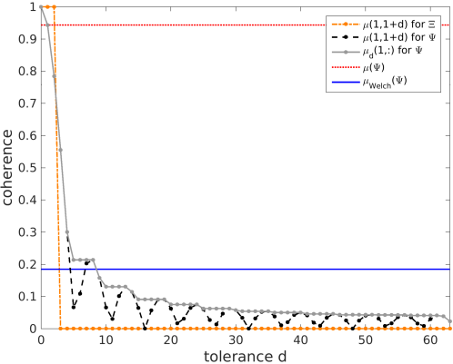
Define the set of $d$-spread coefficients (with wrapping) as $$\Gamma_{d}:=\{(i,j)\in[N]^{2}:|i-j|>d,|i-j-N|>d,|i-j+N|>d\}.$$ Then the $d$-coherence of a matrix $\Phi$ is defined as $\displaystyle\mu_{d}(\Phi):=\max_{(i,j)\in\Gamma_{d}}\mu(\phi_{i},\phi_{j})\;.$ (7) If $\mu_{d}(\Phi)$ is close to the Welch bound for a certain $d$, we call $\Phi$ $d$-incoherent. For $d=0$ the definition of $\mu_{d}(\Phi)$ coincides with that of the coherence. As $d$ increases $\mu_{d}(\Phi)$ decreases monotonically. Indeed, suppose $f<d$. Then $\displaystyle\mu_{d}(\Phi)=\max_{(i,j)\in\Gamma_{d}}\mu(\phi_{i},\phi_{j})<\max_{(i,j)\in\Gamma_{f}}\mu(\phi_{i},\phi_{j})=\mu_{f}(\Phi),$ where the inequality holds because every $d$ separated set is also $f$ separated, i.e. $\left|\Gamma_{d}\right|<\left|\Gamma_{f}\right|$ with cardinality $\left|\cdot\right|$. With $d$-coherence we can ensure that large column correlations are confined to column indices in the $d$-closure of the reference column. This leads to two key aspects for any successful $d$-tolerant recovery: 1. A large $d^{\prime}$-coherence for all $d^{\prime}<d$ increases noise stability by increasing the number of "distorted copies" of any reference column. 2. A minimal $\tilde{d}$-coherence for all $\tilde{d}>d$ ensures reconstruction of any support elements of mutually disjoint $d$-closures. Figure 1: The advantageous fast decrease of column correlations, $\mu(i,i+d)$, of the first and (1+d)th column for $\Psi$ (dashed, black) and $\Xi$ (dash-dotted, orange) highlights the suitability of those matrices for d-tolerant recovery which is based on $\mu_{d}$ (solid, gray; envelope). The matrices are defined in Section III and were instantiated with $M=24,N=128$. The coherence $\mu(\Psi)$ (dotted, red) and Welch bound $\mu(\Psi)$ (solid blue) are given as references towards classical CS and the least coherence possible for a matrix of these dimensions. Symmetric boundary conditions apply for omitted columns. To provide explicit examples, we consider two matrices, $\Xi$ and $\Psi$, defined as follows. Let $\Psi\in\mathbb{C}^{M\times N}$ be the sensing matrix that equals $F_{N}$ restricted to the first $M$ rows, and let $\Xi\in\mathbb{C}^{M\times N}$ be the sensing matrix that equals $F_{M}$ inflated by $(2d+1)$; in other words, every column of $F_{M}$ is copied $2d$ times to form a consecutive block of $(2d+1)$ columns in $\Xi$. In Fig. 1 direct column correlations $\mu(1,1+f)$ of the first with the $(1+f)$th column are shown for $\Psi$ (dashed, black) and $\Xi$ (dash-dotted, orange). Note, only half of the range is shown, as the other half is mirrored. Since both $\Psi$ and $\Xi$ are directly derived from the Fourier matrix, they inherit the invariance property of the column correlations with shifting reference index $j$, $$\forall j\in\left[N\right]:\forall f\in\mathbb{N}_{0}\;\text{such that}\;\mu(1,1+f)=\mu(j,j+f)\;.$$ (8) Thus the shown correlation pattern is exemplary for any column index. For $\Xi$ this is only true for every $(2d+1)$th column. If $\Xi$ is constructed with a fixed $(2d+1)=3$ inflation, we observe $3$ columns with $\mu(1,1+f)=1$. Those are the first column and its copies. For all columns further away $\mu(1,1+f)=0$ due to the orthogonality of the columns in $F_{M}$. Since it is at least for every $(2d+1)=n$th column $\mu(n,n+d)=\mu_{d}(\Xi)$ for this matrix construction, we have maximal $d>d^{\prime}$-coherence and minimal $d<\tilde{d}$-incoherence. To incorporate noise robustness, large $d^{\prime}$-coherences that are still unequal to $1$ are preferable. The greater the deviation from $1$, the larger the noise tolerance. This statement is however limited. Allowing for too much noise compensation would allow a $d$-tolerant reconstruction to completely fail. Experimentally it was found that for OMP a $d$-coherence larger than $0.75$ is beneficial. Due to row restrictions from $F_{N}$ as one continuous block in the case of $\Psi$, we see that large column correlations are possible that are not equal to $1$. Since the coherence $\mu(\Psi)$ (dotted, red) is large, from the perspective of conventional CS theory this matrix seems not to be suited for reconstruction. Matrices used in CS are usually required to have a coherence that is close to the Welch bound, $\mu_{\text{Welch}}(\Psi)$ (solid, blue). We can see however that although correlations of neighboring columns in $\Psi$ are large, the level of correlation rapidly drops with increasing distance between the regarded columns. This means the matrix is only partially coherent and well suited for $d$-tolerant recovery. For $d>8$ (for $M=24,N=128$) it is even $\mu_{d}(\Psi)<\mu_{\text{Welch}}(\Psi)$ motivating the hope that if existing incoherent theory could be adapted to $d$-incoherent theory in a similar way, then it would be possible to get an even better performance in $d$-tolerant recovery than the incoherent theory would allow for a perfectly incoherent sensing matrix. This behavior is well captured by the $d$-coherence (solid, gray). So more specifically $\Psi$ is $\tilde{d}$-incoherent with $\tilde{d}>8$ and could be considered $d^{\prime}$-coherent for $d^{\prime}\leq 3$. Qualitatively this means that in theory, noise robust reconstruction of $S$-sparse signals with small dynamic range, up to an SNR of $0.87$ (equal to $0.45$ of linear independence) with $d=3$ and $S=S_{\text{max}}=18$ from $M=24$ measurements would be possible. In numerical experiments based on OMP and complex valued signals with arbitrary range, this translates into a $3$-tolerant recovery of $6$ more non-zeros on average by using the coherent matrix $\Psi$ instead of an incoherent matrix (random row restricted submatrix of $F_{N}$ of size $M\times N$). To recover at least the same amount of non-zeros with incoherent matrices as with partially coherent matrices and $d=3$, the tolerance would have to be increased to $d\geq 8$. This is true for any SNR in the range of $[0,\infty]$.

3.2 Additional definitions

In this section we introduce a collection of other important concepts that help characterizing the $d$-tolerant recovery setup. We begin with generalizing the concept of the aforementioned column correlation invariance, (8), of Fourier submatrices obtained by row selection. The distribution of highly correlated columns within $\Phi$ can be characterized in terms of matrix coherence functions.

Definition 3

The set of matrix coherence functions $\left\{\mu^{(j)}\right\}_{j\in\left[N\right]}$ of a matrix $\Phi\in\mathbb{C}^{M\times N}$ is defined through $\displaystyle\mu^{(j)}:=\left(\mu\left(\phi_{j},\phi_{1}\right),\dots,\mu\left(\phi_{j},\phi_{N}\right)\right)\,.$ (9) With the help of the matrix coherence functions, two fundamentally different types of partially coherent matrices can be distinguished.

Definition 4

A set of matrix coherence functions is called dynamic, if the correlation of any column with the reference column depends only on the difference of the column indices. Otherwise a set of matrix coherence functions is called static. The choice of the terminology static and dynamic is motivated by the simple cases (i) when all neighboring columns are highly correlated the coherence functions can be viewed via the gram matrix $\Phi^{*}\Phi$ and appear as a sliding gradient (dynamic), e.g. $\Phi\equiv\Psi$, whereas (ii) when the matrix contains blocks of correlated columns and columns in different blocks are uncorrelated, the gram matrix consists of a rigid series of blocks (static), e.g. $\Phi\equiv\Xi$. A similar $d$-tolerant extension as was made to the coherence can be made to the cumulative coherence (also known as $\ell_{1}$-coherence or the Babel function). It will be used in the proof of Theorem 9. The cumulative $d$-coherence is one way to quantify the correlations of any given element with a consecutive, disjoint block of length at most $2d+1$.

Definition 5

For $\Phi\in\mathbb{C}^{M\times N}$, we define its cumulative $d$-coherence $\mu^{C}_{d}(\Phi,k)$ with test-set cardinality $k$ as: $\displaystyle\mu^{C}_{d}(\Phi,k)$ $\displaystyle:=\max_{\begin{subarray}{c}\Gamma\subset\left[N\right]\\ \left|\Gamma\right|=k\end{subarray}}\max_{i\notin\text{clos}_{d}\left(\Gamma\right)}\sum_{j\in\Gamma}\frac{\left|\left<\phi_{i},\phi_{j}\right>_{2}\right|}{\left\lVert\phi_{i}\right\rVert_{2}\left\lVert\phi_{j}\right\rVert_{2}}\,.$ (10) We write $\mu^{C}(\Phi,k):=\mu^{C}_{0}(\Phi,k)$ for the standard cumulative coherence. It is easy to see that the cumulative $d$-coherence satisfies the following properties: • $\mu^{C}_{d}(\Phi,k)$ is monotonically decreasing as $d$ increases. Indeed, we have for any $f<d\in\mathbb{N}_{0}$: $$\mu^{C}_{d}(\Phi,k)\leq\mu^{C}_{f}(\Phi,k)\leq\mu^{C}(\Phi,k)\,.$$ (11) • $\mu^{C}_{d}(\Phi,k)$ is monotonically increasing as $k$ increases: $$\forall k<l\in\mathbb{N}_{0}:\mu^{C}_{d}(\Phi,k)\leq\mu^{C}_{d}(\Phi,l)\,.$$ (12) • The lower bound given in Theorem 5.8 of [2] applies by replacing $N$ by $\hat{N}:=\max\left\{M,\left\lceil\frac{N}{d}\right\rceil\right\}$. That is: $$k\leq\sqrt{\hat{N}-1}\xRightarrow[\phantom{bla}]{}\mu^{C}_{d}(\Phi,k)\geq k\sqrt{\frac{\hat{N}-M}{M(\hat{N}-1)}}\,.$$ (13)

4 Numerical simulation results

In this section we demonstrate the advantage of coherence in $d$-tolerant recovery using numerical simulation results. The main part of the results is based on the $d$-tolerant recovery measure, (3). Results shown in Fig. 6 and Fig. 7 were produced using MATLAB 2017a [32] with the median of 100 iterations per data point. All other results shown below are obtained via standard OMP with MATLAB 2015b [32] using the RPECS Matlab toolbox (version 1.1) [33] and with the median of $500$ iterations per data point. For each iteration just the signal and the noise were re-initialized. The matrices were newly initialized for each set of parameters only. All generated signals were complex valued. Their support was uniformly random distributed. The amplitudes of the real and imaginary parts were selected i.i.d. for every non-zero, uniformly at random on $[-50,50]$. The noise entries were i.i.d. standard normally distributed and then rescaled to fit the desired signal-to-noise ratio (SNR). Note that we do not force the signal to have spread support unless explicitly stated. We consider several types of sensing matrices, given as: F_consecBegin: The first $M$ consecutive rows of $F_{N}$. (Called $\Psi$ in Section 3.1.) F_consecutive: Any $M$ consecutive rows of $F_{N}$. The shift of the block was uniformly random distributed and selected from $\left[1,N-M\right]$. F_rand: $M$ rows of $F_{N}$ were selected uniformly at random. F_nXStatBlocks: Uses $5\left\lfloor\log{N}\right\rfloor$ blocks of consecutive columns from F_consecutive, constructed from $F_{3N}$. R_gauss: Gaussian random matrix. All matrices were $\ell_{2}$-column normalized. The incoherent matrices are F_rand and R_gauss, and the partially coherent matrices are F_consecBegin, F_consecutive and F_nXStatBlocks. F_nXStatBlocks is an approximation to a matrix with static matrix coherence function. The coherence across the column blocks will be low and thus the matrix will appear to have almost rigid blocks of high coherence.

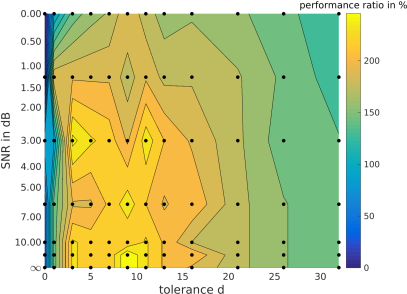
(a) $N=1024$

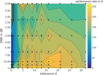
(b) $N=2048$

Figure 2: Consider the percentage of non-zeros recovered with respect to the $d$-tolerant recovery measure. Let $X$ be the percentage recovered with a partially coherent sensing matrix (F_consecutive) and $Y$ the percentage recovered with an incoherent sensing matrix (F_rand). The plot shows the ratio $X/Y$ and as such the benefit of coherent sensing for varying tolerances $d$ and amounts of noise. The number of measurements, $M=32$, the sparsity, $S=16$, and the signal dimension, $N$, are fixed within each plot. Shown in Fig. 2 are the ratios of the percentages of non-zeros that could be recovered, $d$-tolerant wise, with a partially coherent sensing matrix (F_consecutive) over an incoherent sensing matrix (F_rand). The color bar represents the ratio in recovery percentages; thus, when the color is greater than $100\%$ we see improvements with our method. The presented situations are heavily undersampled with the number of measurements $M=32$ fixed and $N=1024$ or $N=2048$. In both plots, we see an optimal value for the tolerance $d$. More importantly, we observe improvements from coherence (i.e. when the ratio percentage is above 100) for a broad range of values of $d$, especially in the mild SNR regime. Only if $d=0$ incoherent matrices perform like partially coherent sensing matrices. Unsurprisingly, this means that for exact support recovery the incoherent sensing is similar or better (for small undersampling factors $N/M\leq 4$, see discussion of Fig. 4 below) in determining the position of every non-zero.

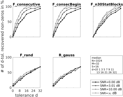
(a) $N/M=1024/32$

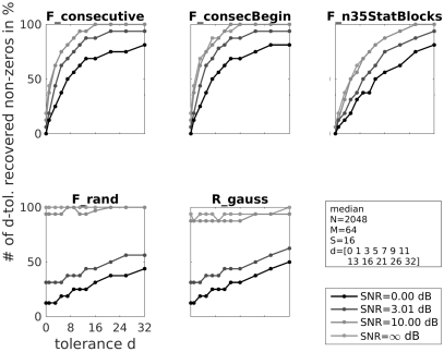
(b) $N/M=2048/64$

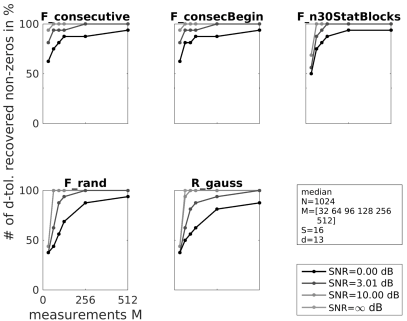
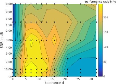
Figure 3: The advantage of coherent (top) over incoherent sensing matrices (bottom) is illustrated in terms of percentages of $d$-tolerant recovered non-zeros via OMP for an increasing tolerance $d$ and several noise levels. The undersampling factor is fixed at $N/M=32$ and the sparsity is $S=16$. Figure 3 shows the average number of $d$-tolerantly recovered non-zeros as a function of $d$, for various types of sensing matrices, various noise levels, and only few measurements ($N/M=32$). We consider $N/M=1024/32$ in Fig. 3a first. The partially coherent sensing matrices F_consecutive and F_consecBegin (with dynamic matrix coherence functions) perform especially well. Most importantly, already with small values of $d$ ($\approx 5$) much more non-zeros can be reconstructed. If little noise is present ($\text{SNR}\leq 10$dB), for $d=9$ the number of reconstructed non-zeros is doubled for partially coherent versus incoherent sensing. Close to $100\%$ recovery is reached for $d>16$ in the low noise setting. Figure 3b with $N/M=2048/64$ shows what happens if both the signal dimension and the number of measurements get scaled up. Due to the lower normalized sparsity $S/M=0.25$ incoherent sensing matrices are able to perform well for large SNR’s ($\geq 10$dB). As the amount of measurement noise increases the incoherent matrices are however drastically impacted ($31\%$ instead of $\approx 100\%$ for $d=0$, $\text{SNR}=3.01$dB for both incoherent matrices). The impact of noise on the coherent sensing matrices is much less severe especially for $d\geq 7$. This emphasizes that partially coherent sensing matrices can be employed very effectively at their optimal level of incoherence for challenging signal detection situations. The percentage of $d$-tolerantly recovered non-zeros is in general monotonic with increasing $d$ amongst all the sensing matrices. Therefore, selecting a large value for $d$ will not result in substantially worse recovery. This general rule coincides with intuition. For (almost) exact support reconstruction ($d\in\left\{0,1\right\}$) using coherence is irrelevant or even bad in the heavily under-sampled setting throughout all SNR levels. Figure 4: Even with an increasing number of measurements, the coherent (top) dominate the incoherent sensing matrices with respect to the percentage of d-tolerant recovered non-zeros via OMP for various noise levels. The signal dimension, the sparsity, and the tolerance are fixed at $N=1024$, $S=16$, and $d=13$. Figure 4 depicts the trends in $d$-tolerant support recovery for an increasing number of measurements $M$ while $N$ is fixed, for various types of sensing matrices, and for various noise levels. Again F_consecutive and F_consecBegin perform especially well. Coherent sensing matrices make much better use of additional, possibly very distorted, measurements, as soon as a certain tolerance (e.g. $d=13$) in the signal support is allowed. For larger numbers of measurements $M\geq 256$ incoherent sensing matrices perform similarly well, independent of the SNR. This again underlines that partially coherent sensing matrices are especially interesting for applications in which using few measurements is key. Figure 5: Extended regions with more then twice as many d-tolerant recovered non-zeros using coherent versus incoherent sensing matrices are shown in the analogue of Fig. 2a for the special case of signals that have their non-zeros never closer then $(4d+1)$. Since we will consider in Section 5 only signals that have their non-zeros never closer then $(4d+1)$, we provide results for those signals in Fig. 5, in analogy to Fig. 2. Next, we compare the coherent sensing paradigm to the simple subsampling strategies described in Section 2.1. Unsurprisingly, the second two naive approaches described there yield very poor results and are not even competitive. Figure 6 displays the results for the “Subsampling on coarse grid” approach; using the standard OMP reconstruction method. The notation $F_{R}$ indicates the rows were subsampled at random, and $F_{cB}$ indicates they were selected to be the first $M$ consecutive rows. Since $d$ is typically much smaller than $N$, both types of sampling approaches are in some sense coherent, so it is not surprising that both are somewhat comparable. Our design, however, maintains the signal on a finer grid, which induces slightly more coherence, which is evident in the improved reconstruction.

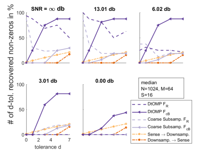
(a) $N/M=1024/64$

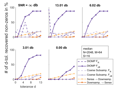
(b) $N/M=2048/64$

Figure 6: A comparison of the proposed DtOMP, Algorithm 1, with the other methods outlined in Section 2.1 reveals that out of these options using the coherent sensing matrix, $F\_consecBegin$ ($F\_cB$) with DtOMP, recovers the largest percentage of non-zeros with a certain d-tolerance as soon as considerable noise is present (top) and/or the undersampling ratio is increased drastically (bottom). $F\_rand$ ($F\_R$) was the chosen representative for incoherent matrices. In this paper we have focused on greedy methods for simplicity of the analysis, but for completeness we include some results using convex methods for reconstruction, Fig. 7. In particular, we compare the results using the proposed DtOMP, Algorithm 1, against Basis Pursuit Denoising (using SPGL1). We see similar trends and behavior in terms of the tolerant $\ell_{2}$-error measure, Fig. 7a, but from the number of tolerant recovered non-zeros its clear that actually often the greedy approach outperforms the convex method, Fig. 7b. The reason for this behavior are multiple false positives in the case of the convex method. Note especially that the typical partially coherent sensing matrix $\text{F}_{\text{cB}}$ has an advantage over the incoherent matrix $\text{F}_{\text{R}}$ when noise is present and tolerant recovery is the objective. However, we emphasize once again that the OMP-based reconstruction method is likely still not optimal, and that further study should be done to analyze reconstruction performance under this new paradigm of beneficial coherent sensing.

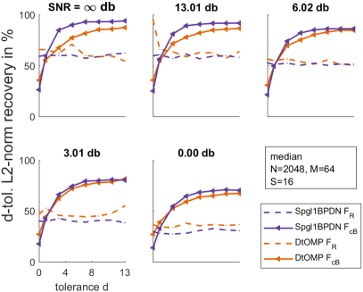
(a)

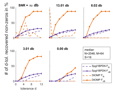
(b)

Figure 7: Convex methods such as SPGL1 BPDN are comparable to DtOMP in terms of tolerantly recovered intensity but not in percentages of $d$-tolerant recovered non-zeros for large undersampling ratios of $N/M=32$, irrespective of the measurement noise and tolerance chosen. We close with a remark on the $d$-tolerant $\ell_{2}$-norm error based recovery measure $\rho_{2}$, introduced below. Finding such a measure is not trivial but may be desired for classification of the magnitude differences of reconstruction and true signal. We choose a measure that requires knowledge about the true signal and is evaluated in two steps: First, we create new proxy signals $x_{p},\tilde{x}_{p}$ via: $\displaystyle(x_{p})_{i}$ $\displaystyle=\begin{cases}\sum_{j\in\text{clos}_{d}\left(i\right)}\left|x_{j}\right|,&\text{if }i\in\text{supp}\left(x\right)\\ 0,&\text{otherwise}\end{cases}$ (14a) $\displaystyle(\tilde{x}_{p})_{i}$ $\displaystyle=\begin{cases}\sum_{j\in\text{clos}_{d}\left(i\right)}\left|\tilde{x}_{j}\right|,&\text{if }i\in\text{supp}\left(x\right)\\ 0,&\text{otherwise}\;.\end{cases}$ (14b) For example, if $x=(1,0,1,0,0,1,1,0,0)$ and $d=2$, we have $x_{p}=(2,0,2,0,0,2,2,0,0)$. Note that we sum over the same set of indices in both cases, which causes both proxy signals to share the same support. In a second step we compute $$\rho_{2}(\tilde{x}_{p},x_{p}):=1-\frac{\left\lVert\tilde{x}_{p}-x_{p}\right\rVert_{2}}{\left\lVert\tilde{x}_{p}\right\rVert_{2}\left\lVert x_{p}\right\rVert_{2}}\;.$$ (15)

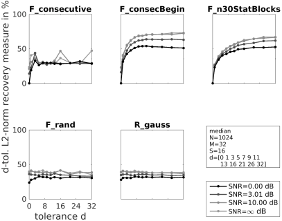
(a) $M=32$

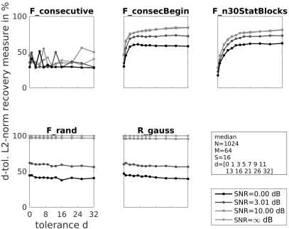
(b) $M=64$

Figure 8: Incoherent (bottom) can compete with coherent sensing matrices (top) in terms of the $d$-tolerant recovered $\ell_{2}$-norm only if the undersampling ratio is comparatively low, $N/M=16$, and the measurement noise is low as well. For harsher sensing conditions $F\_consecBegin$ usually gives the best performance as well. For that recovery measure we find incoherent sensing matrices are favorable for any SNR and $M\in[64,256)$, i.e. a normalized sparsity smaller than $S/M\leq 0.25$ and an undersampling factor larger than $N/M\geq 4$. This is depicted exemplary in Fig. 8 for $S/M=0.5$ in Fig. 8a and $S/M=0.25$ in Fig. 8b. For F_consecBegin and F_nXStatBlocks we observe the same low impact of measurement noise and about $50\%$ recovery as soon as the tolerance is set sufficiently large, $d\geq 7$. We notice F_consecBegin is slightly better than F_nXStatBlocks but F_consecutive produces a much weaker and highly inconclusive result. This is due to the different construction of F_consecBegin and F_consecutive. Both share exactly the same coherence pattern (absolute value) but in general only the former has a smoothly varying phase difference among the real and imaginary parts of the columns. The latter experiences rapid phase shifts in real and imaginary part from column to column. Thus an approximate $d$-tolerant reconstruction can have a quite different magnitude even though reconstructed columns are largely correlated to the true support. Nevertheless, the findings for F_consecBegin and F_nXStatBlocks stress that it is not only possible to better reconstruct the approximate support but also the approximate magnitude by using coherent sensing matrices in difficult sensing scenarios. With a smaller undersampling factor, e.g. $N/M\geq 4$, the results (not depicted here) of in-/coherent sensing matrices largely coincide again. This nicely complements the observations made above: For very few (possibly noisy) measurements, partially coherent sensing matrices give a better reconstruction both in support and magnitude. But in the typical CS setting with exact recovery with respect to the $\ell_{2}$-norm and a moderately low number of measurements, incoherent sensing matrices successfully prevail.

5 Analytical Justification

In this section we provide initial guarantees for the $d$-tolerant recovery of $S$-sparse signals without measurement noise through an OMP-like algorithm using partially coherent sensing matrices. We will utilize the notion of spread support.

Definition 6 ($d$-spread set)

A set $B$ is $d$-spread, if $$\forall i\neq j\in B:\enskip\left|i-j\right|>d\;.$$ (16) A signal $x$ is said to have a $d$-spread support, if $\text{supp}\left(x\right)$ is a $d$-spread set. For the purpose of this work, sufficiently spread means a signal has a $(4d+1)$-spread support. This allows us to ignore recombinations of multiple non-zeros to a single representative during reconstruction and enables us to prove results following closely the initial contributions made for robust recovery via standard OMP. The line of theorems we follow is based on the exact recovery condition (ERC). Within the spread signal support setting only minor adjustments to the theorems are necessary in the noiseless scenario to ensure validity for $d$-tolerant recovery with partially coherent sensing matrices. Further, the OMP-like algorithm has been empirically found to perform similar to OMP in this setting with and without measurement noise. The method below is an adaptation of OMP, which is similar to Band-Excluded OMP in [16], in the context of “coherence bands”.

5.1 Algorithm

To account for the ban of recombinations in the OMP algorithm we forbid new candidates for the reconstructed support to be selected from the $2d$-closure of the already reconstructed support, as shown in Algorithm 1. This modification ensures that every high coherence neighborhood is met exactly once and since we will assume a $(4d+1)$ spread for our signals in the statements of the next section, we can guarantee not to miss any non-zero by this exclusion. Algorithm 1 Pseudo code for d-tolerant OMP (DtOMP) 1:$y\in\mathbb{C}^{M}$, $S\in\mathbb{N}^{+}$, $\Phi\in\mathbb{C}^{M\times N}$, $d\in\mathbb{N}_{0}$ 2:$d$-tolerant recovery $\tilde{x}\in\mathbb{C}^{N}$ 3:$k=0$, $x^{k}=0$, $\Sigma=\left\{\right\}$, $r^{(0)}=y$ $\triangleright$ Initialization 4:while $k\leq S$ and $\left|\Sigma\right|<S$ do 5:     $k=k+1$ 6:     $b=\left|\Phi^{*}r^{(k-1)}\right|$ 7:     $\tilde{n}=\operatorname*{argmax}_{n\notin\text{clos}_{2d}\left(\Sigma\right)}\left\{b_{n}\right\}$ $\triangleright$ Modification 8:     $\Sigma=\Sigma\cup\left\{\tilde{n}\right\}$ 9:     $x^{(k)}_{\Sigma}=\Phi^{\dagger}_{\Sigma}y$ 10:     $r^{(k)}=y-\Phi x^{(k)}$ 11:end while 12:$\tilde{x}=x^{(S)}$ In the algorithm, $x^{(k)}_{\Sigma}$ and $\Phi^{\dagger}_{\Sigma}$ are the reconstruction in the $k$th iteration restricted to the rows in the set $\Sigma$ and the Moore-Penrose pseudoinverse of $\Phi$ restricted to the columns with indices in $\Sigma$, respectively. Through the exclusion of the $2d$-closures of the already recovered support, the algorithm will select at most one candidate per high correlation region. This modification is negligible within the scenario of signals with $(4d+1)$-spread support as all the numerical experiments for all tested parameter sets showed. For signals without spread support DtOMP fails at exact recovery by design due to its exclusion feature.

5.2 Theory

Here we present some results closely related to established results for recovery from coherent sampling. These, like others in the literature, are for signals with spread support only. As our experiments seem to indicate, we conjecture this condition is only an artifact of the proofs, and further study should be performed to remove this assumption. The given theoretical reconstruction guarantees are a close analog to the ERC based incoherent OMP theory [6, 16]. The presented results can be understood as a characterization of OMP in the noiseless scenario of signals with sufficiently spread support. Before we formulate the theorems we need to fix the notion of a $d$-approximate pair of sets $\left\{\Sigma,\Gamma\right\}_{d}$.

Definition 7

Let $\Sigma,\Gamma\subset\mathbb{N}^{+}$ be sets and a $d\in\mathbb{N}_{0}$ be given. Then we have a $d$-approximate pair of sets $\left\{\Sigma,\Gamma\right\}_{d}$, if and only if $$\Sigma\subseteq\text{clos}_{d}\left(\Gamma\right)\;\text{and}\;\Gamma\subseteq\text{clos}_{d}\left(\Sigma\right)\;,$$ (17) that is their distance in the Hausdorff-metric is at most $d$. We will call the set of all such pairs of sets containing at least one set of cardinality $S$, $\mathcal{D}^{S}_{d}$. The following theorem is the essential result ensuring recovery from noiseless measurements via the $d$-tolerant recovery condition (TRC). We do not present a proof here, since it follows similarly to previously established results [6, 16]. In particular, see Theorem 1 of [16] for a more general result that tolerates noise and is in terms of arbitrary coherence bands, rather than $d$-tolerant recovery.

Theorem 8 ($d$-tolerant recovery guarantee without measurement noise).

Consider (1) with $e=0$ and $\left|x\right|_{0}\leavevmode\nobreak\ =\leavevmode\nobreak\ S$. The $d$-tolerant reconstruction of the signal can be guaranteed via DtOMP, Algorithm 1, if: $\displaystyle\text{supp}\left(x\right)\text{ is $(4d+1)$-spread}$ (18a) $\displaystyle\mu_{d}(\Phi)\leq\text{const.}\ll 1$ (18b) $\displaystyle\forall\left\{A,B\right\}_{d}\in\mathcal{D}^{S}_{d}:\enskip A\text{ is $(4d+1)$-spread},\;\tilde{T}:=A\cup B,$ $\displaystyle\hskip 40.00006ptT:=\text{clos}_{2d}\left(A\right)\;\xRightarrow[\phantom{bla}]{}\;\max_{j\in T^{C}}\left\lVert\Phi_{\tilde{T}}^{\dagger}\phi_{j}\right\rVert_{1}<1$ (TRC) where $\left\{A,B\right\}_{d}$, $\mathcal{D}^{S}_{d}$ are given in Definition 7 and $\mu_{d}(\Phi)$ is given in (7). The theorem allows to guarantee the $d$-tolerant recovery of any $S$-sparse signal from noiseless measurements using partially coherent sensing matrices. The original theory for OMP will fail for partially coherent sensing matrices since the ERC is usually not satisfied. In addition, given that the utilized sensing matrix has large $d^{\prime}$-coherences ($d^{\prime}<d$) in every $d$-neighborhood, the reconstruction will naturally be also close in magnitude. Note that many naturally arising sensing matrices such as overcomplete Fourier frames satisfy the condition of the theorem for some $d$. This can be seen in Fig. 1 for the example of $\Psi$. The TRC will hold for any sufficiently small $\mu_{d}(\Phi)$ since the Hausdorff distance between $T^{C}$ and $\tilde{T}$ is by construction larger then $d$. We also point out that (18b) is primarily a lower bound on the minimal number of measurements $M$. This link is established using the Welch bound applied to all possible submatrices restricted to column indices that are $(4d+1)$-spread. Continuing the theoretical construction as in [6], one can ensure the TRC by imposing conditions on the cumulative coherence.

Theorem 9 (TRC guarantee).

Let $\Phi\in\mathbb{C}^{M\times N}$. Then the TRC holds for all $\left\{A,B\right\}_{d}\in\mathcal{D}^{S}_{d}$, if $\displaystyle\mu^{C}_{d}(\Phi,2S-1)+\mu^{C}_{d}(\Phi,2S)<1\;,$ (19) where $\left\{A,B\right\}_{d}$, $\mathcal{D}^{S}_{d}$ are given in Definition 7 and $\mu^{C}_{d}(\Phi,\cdot)$ is given in (10).

Proof.

The proof follows analogously to the proof of Theorem 3.5 in [6] with only minor modifications. Namely $S$ is replaced with $2S$, since the optimal support of that theorem is replaced by the union $A\cup B$ of two $S$-cardinal sets, and $\mu^{C}(\Phi,\cdot)$ is replaced by $\mu^{C}_{d}(\Phi,\cdot)$. ∎

Corollary 10

Equation (19) of Theorem 9 holds, with the conditions stated, if any of the following inequalities is satisfied: $\displaystyle S$ $\displaystyle<\frac{1}{4}\left(\mu_{d}(\Phi)^{-1}+1\right)$ (20) $\displaystyle\mu^{C}_{d}(\Phi,2S)$ $\displaystyle<\frac{1}{2}\;.$ (21)

Proof.

Both conditions follow from the monotonic behavior of $\mu^{C}_{d}(\Phi,\cdot)$. Equation (20) is proved using $$\mu^{C}_{d}(\Phi,k)\leq\mu_{d}(\Phi)k\;,$$ (22) which holds due to the monotonic increase of $\mu^{C}_{d}(\Phi,k)$ as $k$ decreases. So we have: $\displaystyle\mu^{C}_{d}(\Phi,2S-1)+\mu^{C}_{d}(\Phi,2S)$ $\displaystyle\stackrel{{\scriptstyle\mathclap{\eqref{eq:lemma_coherences_lb_mu_d}}}}{{\leq}}\left(2S-1+2S\right)\mu_{d}(\Phi)<1$ $\displaystyle\iff S<\frac{1}{4}\left(\mu_{d}(\Phi)^{-1}+1\right)\;.$ Equation (21) follows immediately from the increasing behavior of $\mu^{C}_{d}(\Phi,k)$: $\displaystyle\mu^{C}_{d}(\Phi,2S-1)+\mu^{C}_{d}(\Phi,2S)$ $\displaystyle\leq 2\mu^{C}_{d}(2S,\Phi)<1$ $\displaystyle\iff\mu^{C}_{d}(2S,\Phi)<\frac{1}{2}\;,$ completing the proof. ∎ Both results given in the corollary are stronger than the original requirement but may be easier to verify. As is the case for OMP, (20) is stronger than (21). As a concrete example of a matrix that satisfies the conditions of the corollary, one could consider $F\_consecBegin$; when $N=1024$, $S=1$, and $M=64$, the conditions hold for $13\leq d\leq 23$. When $N=512$, $S=2$, and $M=64$, the conditions hold for $15\leq d\leq 20$. Clearly these are not optimal conditions, but do provide a heuristic that holds for practical sensing matrices in certain parameter regimes. Moreover, we see tolerant support recovery for much broader ranges in the experiments.

6 Conclusion and future directions

We considered $d$-tolerant recovery and showed that in the low and noisy measurement regime, coherence in the sensing matrix is actually beneficial – despite just the opposite in the classical recovery setting. We have taken first steps towards developing a framework and building a theoretical foundation for $d$-tolerant recovery. An empirical characterization of OMP for the purpose of $d$-tolerant recovery has been provided. It was backed for signals with sufficiently spread support theoretically through the interim modified OMP, termed DtOMP, which was found to be empirically the same as OMP in this setting. A comparison with simpler downsampling alternatives and the convex SPGL1 BPDN algorithm underlined our findings and showed best performance, both with respect to tolerant support and tolerant magnitude recovery, for partially coherent sensing matrices when paired with DtOMP. The modifications necessary for the ERC based OMP reconstruction guarantees were minimal. We introduced a modified version of the ERC, called TRC, with which we were able to prove $d$-tolerant recovery of arbitrary $S$-sparse signals with $(4d+1)$ spread support from noiseless measurements using partially coherent sensing matrices. For noisy recovery the classic proofs can not be easily extended. Some future directions include: (i) developing new prove strategies to proof recovery guarantees for the noisy measurement setting; (ii) deriving theoretical guarantees of the $d$-tolerant reconstruction for signals without a spread support; (iii) analyzing the coherent sensing paradigm for other algorithms in order to improve the reconstruction performance; (iv) deriving a characterization of the phase transition of $d$-tolerant algorithms, to enable clear assertions whether partially coherent or incoherent sensing should be employed given the problem dimensions; (v) further investigating how the smallest "optimal" value of $d$ relates to the problem dimensions and the coherence levels in the matrix in general; (vi) the development of partially coherent sensing matrices specifically designed for particular applications. (vii) a study utilizing a variant of the restricted isometry property may be illuminating in the context of tolerant recovery, see [20] for some initial considerations in this direction.

Acknowledgments

We would like to thank Omer Bar-Ilan, whose Master thesis inspired this work, the Faculty of Mathematics and Informatics of TU Bergakademie Freiberg for providing computational resources. The work of T. Birnbaum was supported in part by the INTERFERE ERC Consolidator Grant. The work of Y. C. Eldar was supported in part by the European Union’s Horizon 2020 Research and Innovation Program through the ERC-BNYQ Project, and in part by the Israel Science Foundation under Grant 335/14. The work of D. Needell was supported by NSF CAREER grant $\sharp$1348721 and the Alfred P. Sloan Foundation.

- [1] Yonina C. Eldar and Gitta Kutyniok. Compressed Sensing: Theory and Applications. Cambridge University Press, 2012.
- [2] Holger Rauhut Simon Foucart. A Mathematical Introduction to Compressive Sensing. Applied and Numerical Harmonic Analysis. Springer New York, 2013. doi:10.1007/978-0-8176-4948-7.
- [3] Y. C. Eldar. Sampling theory: Beyond bandlimited systems. Cambridge University Press, 1 edition, 2015.
- [4] David L. Donoho and Philip B. Stark. Uncertainty principles and signal recovery. SIAM Journal on Applied Mathematics, 49(3):906–931, Jun 1989. doi:10.1137/0149053.
- [5] Emmanuel J. Candes and Terence Tao. Near-optimal signal recovery from random projections: Universal encoding strategies? IEEE Transactions on Information Theory, 52(12):5406–5425, Dec 2006. doi:10.1109/TIT.2006.885507.
- [6] Joel A. Tropp. Greed is good: algorithmic results for sparse approximation. IEEE Transactions on Information Theory, 50(10):2231–2242, Oct 2004. doi:10.1109/TIT.2004.834793.
- [7] O. Bar-Ilan and Y. C. Eldar. Sub-Nyquist radar via Doppler focusing. IEEE Transactions on Signal Processing, 62(7):1796–1811, Apr 2014. doi:10.1109/TSP.2014.2304917.
- [8] Joel A. Tropp, Anna C. Gilbert, Sambavi Muthukrishnan, and Martin J. Strauss. Improved sparse approximation over quasi-incoherent dictionaries. In International Conference on Image Processing, Proceedings., volume 1, pages I–37–40, Sep 2003. doi:10.1109/ICIP.2003.1246892.
- [9] David L. Donoho, Michael Elad, and Vladimir N. Temlyakov. Stable recovery of sparse overcomplete representations in the presence of noise. IEEE Transactions on Information Theory, 52(1):6–18, Jan 2006. doi:10.1109/TIT.2005.860430.
- [10] Emmanuel Candes and Justin Romberg. Sparsity and incoherence in Compressive Sampling. Inverse problems, 23(3):969–985, Nov 2007.
- [11] Moshe Mishali and Yonina C. Eldar. Blind multiband signal reconstruction: Compressed Sensing for analog signals. IEEE Transactions on Signal Processing, 57(3):993–1009, Mar 2009.
- [12] Yonina C. Eldar and Moshe Mishali. Robust recovery of signals from a structured union of subspaces. IEEE Transactions on Information Theory, 55(11):5302–5316, Nov 2009. doi:10.1109/TIT.2009.2030471.
- [13] Guangliang Chen, Atul Divekar, and Deanna Needell. Guaranteed sparse signal recovery with highly coherent sensing matrices. Sampling Theory in Signal & Image Processing, 13(1):91–109, Apr 2014.
- [14] John Wright, Allen Y. Yang, Arvind Ganesh, Shankar S. Sastry, and Yi Ma. Robust face recognition via sparse representation. IEEE Transactions on Pattern Analysis and Machine Intelligence, 31(2):210–227, Feb 2009.
- [15] Omer Bar-Ilan. Sub-Nyquist radar via Doppler focusing. Master’s thesis, The Technion - Israel Institute of Technology, Oct 2014.
- [16] Albert Fannjiang and Wenjing Liao. Coherence pattern-guided Compressive Sensing with unresolved grids. SIAM Journal on Imaging Sciences, 5(1):179–202, Jun 2012.
- [17] Marco F. Duarte and Richard G. Baraniuk. Spectral compressive sensing. Applied and Computational Harmonic Analysis, 35(1):111 – 129, 2013. doi:10.1016/j.acha.2012.08.003.
- [18] Y. C. Eldar, P. Kuppinger, and H. Bolcskei. Block-sparse signals: Uncertainty relations and efficient recovery. IEEE Transactions on Signal Processing, 58(6):3042–3054, Jun 2010. doi:10.1109/TSP.2010.2044837.
- [19] Jun Wang, Gang Li, Hao Zhang, and Xiqin Wang. Analysis of block OMP using block RIP. ArXiv Mathematics e-prints, Apr 2011. URL: arXiv:1104.1071[cs.IT].
- [20] Yuli Fu, Haifeng Li, Qiheng Zhang, and Jian Zou. Block-sparse recovery via redundant block OMP. Signal Processing, 97:162–171, Apr 2014. doi:http://dx.doi.org/10.1016/j.sigpro.2013.10.030.
- [21] Emmanuel J Candes and Yaniv Plan. Near-ideal model selection by l1 minimization. Annals of Statistics, 37(5A):2145–2177, 10 2009. URL: arXiv:0801.0345v3[math.ST], doi:10.1214/08-AOS653.
- [22] Emmanuel J Candes, Yonina C Eldar, Deanna Needell, and Paige Randall. Compressed Sensing with coherent and redundant dictionaries. Applied and Computational Harmonic Analysis, 31(1):59–73, 2011.
- [23] Raja Giryes and Michael Elad. Can we allow linear dependencies in the dictionary in the sparse synthesis framework? In IEEE International Conference on Acoustics, Speech and Signal Processing, pages 5459–5463, May 2013.
- [24] Raja Giryes and Michael Elad. OMP with highly coherent dictionaries. In 10th International Conference on Sampling Theory and Applications (SAMPTA), pages 9–12, Jul 2013.
- [25] R. Rubinstein, T. Peleg, and Michael Elad. Analysis K-SVD: A dictionary-learning algorithm for the analysis sparse model. IEEE Transactions on Signal Processing, 61(3):661–677, Feb 2013. doi:10.1109/TSP.2012.2226445.
- [26] Chris Garnatz, Xiaoyi Gu, Alison Kingman, James LaManna, Deanna Needell, and Shenyinying Tu. Practical approximate projection schemes in greedy signal space methods. ArXiv Mathematics e-prints, pages 1–12, Sep 2014. URL: arXiv:1409.1527[math.NA].
- [27] Simon Foucart. Dictionary-sparse recovery via thresholding-based algorithms. Journal of Fourier Analysis and Applications, 22(1):6–19, May 2016. doi:10.1007/s00041-015-9411-4.
- [28] Emmanuel J Candes and Carlos Fernandez-Granda. Super-resolution from noisy data. Journal of Fourier Analysis and Applications, 19(6):1229–1254, 2013. doi:10.1007/s00041-013-9292-3.
- [29] N. Nguyen and L. Demanet. Sparse image super-resolution via superset selection and pruning. In IEEE Int. Computational Advances in Multi-Sensor Adaptive Processing (CAMSAP), pages 208–211, Dec 2013. doi:10.1109/CAMSAP.2013.6714044.
- [30] Zvika Ben-Haim, Yonina C Eldar, and Michael Elad. Coherence-based performance guarantees for estimating a sparse vector under random noise. IEEE Transactions on Signal Processing, 58(10):5030–5043, Oct 2010. doi:10.1109/TSP.2010.2052460.
- [31] Nam Yul Yu. Deterministic construction of partial Fourier Compressed Sensing matrices via cyclic difference sets. ArXiv Mathematics e-prints, abs/1008.0885, 2010. URL: arXiv:1008.0885[cs.IT].
- [32] MathWorks. Matlab 2015b. Online, 1984. URL: http://www.mathworks.de/products/matlab/.
- [33] Tobias Birnbaum. Rapid prototyping environment for compressed sensing algorithms (RPECS). Online, May 2016. URL: http://de.mathworks.com/matlabcentral/fileexchange/58750-rapid-prototyping-environment-for-compressed-sensing--repcs-.