The driven Dicke Model: time-dependent mean field and quantum fluctuations in a non-equilibrium quantum many-body system

Abstract

We establish a new theoretical framework, based on a time-dependent mean field approach, to address the dynamics of the driven Dicke model. The joint evolution of both mean fields and quantum fluctuations gives rise to a rich and generally non-linear dynamics, featuring a normal (stable) regime and an unstable, super-radiant one. Various dynamical phenomena emerge, such as the spontaneous amplification of vacuum fluctuations, or the appearance of special points around which the mean-field amplitudes rotate during driven time evolution, signalling a dynamical symmetry breaking. We also provide a characterization of the driving-induced photon production in terms of the work done by the driving agent, of the non-adiabaticity of the process and of the entanglement generated between the atomic system and the cavity mode.

The dynamical behavior of quantum critical systems displays interesting features concerning defects or excitations production polkormp ; eisertnatphys , which occurs when the system is driven across its critical point varikz . The Dicke model is a paradigmatic example in this context, embodying a quantum many-body system with highly non-trivial critical features Brennecke ; pnas , where an electromagnetic mode is coupled to a collection of $N$ identical two-levels atoms dicke . Indeed, strong correlations are set both among atoms and with the field, which in turn result in significant non-classical behavior of the radiation and in cooperative effects giving rise to both atomic and photon squeezing.

These tantalising features persist in the case of external driving of the dynamics, as remarkably shown experimentally in Ref. Brennecke , where the corresponding spontaneous symmetry-breaking effect induced by an adiabatic crossing of the quantum critical point of the model has been demonstrated. Non-adiabatic driving has also been the focus of substantive theoretical and experimental investigation varie . In particular, for a periodic driving of the atom–field coupling strength, Ref. Bastidas12PRL108 has shown the emergence of new metastable phases in the driven Dicke model, whose phase diagram appears to be substantially different from the static one, both qualitatively and quantitatively.

In this paper we discuss symmetry breaking and photon generation in the driven Dicke model, where the frequency of the field, the energy of the atoms, and their mutual coupling are all allowed to vary in time. While the dynamical behavior of the single-atom case has been recently studied plenion=1 , we are interested in the thermodynamic limit. By non-adiabatically driving the system, and thoroughly analysing its stability conditions, we highlight implications that non-adiabaticity has on the evolution of both the mean fields and the residual quantum fluctuations. Indeed, the macroscopic trajectories followed by the mean fields are shown to dynamically select one of the symmetry broken configurations each time the critical point is crossed; while the microscopic features of the fluctuations are shown to be crucial for the characterization of the temporal behavior of key observables of the system, such as the photon number. Moreover, we study the thermodynamic work produced by driving the system, and the associated degree of irreversibility, thus addressing the non-adiabatic production of photons from the electromagnetic vacuum, a phenomenon akin to the dynamical Casimir effect Vacanti12PRL108 , and the associated generation of atom-field entanglement, from a genuinely non-equilibrium perspective.

For a negligible mutual atomic interaction and for an atomic system occupying a linear dimension much smaller than the electromagnetic wavelength, the atom field system is described by the collective-spin Hamiltonian $\hat{H}=\hat{H}_{0}+\hat{H}_{int}$ with

$$\hat{H}_{0}=\omega_{a}\hat{a}^{\dagger}\hat{a}+\omega_{b}\hat{J}_{z}\,,\quad\hat{H}_{int}={2g}\left(\hat{a}^{\dagger}+\hat{a}\right)\hat{J}_{x}/\sqrt{N}.$$ (1)

Here $\hat{a}$ ($\hat{a}^{\dagger}$) is a bosonic annihilation (creation) operator, and $\hat{\bm{J}}=(\hat{J}_{x},\hat{J}_{y},\hat{J}_{z})$ is the collective spin operator, with $\hat{\bm{J}}=\sum_{i=1}^{N}{\hat{\bm{\sigma}_{i}}}/{2}$ and $\hat{\bm{\sigma}_{i}}$ is the vector of Pauli spin operators.

As mentioned, we will be interested in the case where $\omega_{a,b}$, and $g$ are all functions of time (in order to avoid notational clutter, and unless otherwise specified, we will avoid writing explicitly any time dependence). In fact, as we discuss below, the key ingredient in the dynamics of the system is the time dependence of the parameter $\mu={\omega_{a}\omega_{b}}/(4g^{2})$. We will treat the atoms as indistinguishable, and consider a fully symmetric initial atomic state. This feature is preserved during time evolution as the symmetric subspace is dynamically invariant. We now consider the Holstein-Primakoff transformation of $\hat{\bm{J}}$ restricted to such subspace and thus introduce the bosonic operators $\hat{b}$ and $\hat{b}^{{\dagger}}$ such that

$$\hat{J}_{z}=\hat{b}^{\dagger}\hat{b}-N/2\,,\quad\hat{J}_{+}\equiv\hat{J}_{x}+i\hat{J}_{y}=\hat{b}^{\dagger}\sqrt{N-\hat{b}^{\dagger}\hat{b}}.$$ (2)

As a result, within the symmetric subspace $\hat{H}_{int}$ takes the form

$$\hat{H}_{int}=g\left(\hat{a}^{\dagger}+\hat{a}\right)\left(\hat{b}^{\dagger}\sqrt{1-\frac{\hat{b}^{\dagger}\hat{b}}{N}}+\sqrt{1-\frac{\hat{b}^{\dagger}\hat{b}}{N}}\hat{b}\right).$$ (3)

In the time-independent case and at the thermodynamic limit, $\hat{H}$ can be diagonalized by isolating from $\hat{b}$ a macroscopic ($\sim\sqrt{N}$) mean contribution Emary03PRE67 and retaining only the leading terms of a $1/N$ expansion of the square roots in Eq. (2), thus obtaining a quadratic Hamiltonian. This procedure implies subtracting a static mean field chosen in order to approximate the Hamiltonian as accurately as possible at low energies, or, loosely speaking, chosen in such a way as to minimize residual quantum fluctuations near the ground state. Our approach to the investigation of the driven model is based on an analogous idea: we will isolate time-dependent mean fields, chosen so as to minimize residual quantum fluctuations around the instantaneous state vector $\left|\psi,t\right\rangle$, whose evolution is generated by an approximately quadratic time-dependent Hamiltonian.

In the thermodynamic limit and for $\mu>\mu_{c}=1$ [$\mu<1$], $\hat{H}$ admits a normal (N) [super-radiant (SR)] quantum phase. At $\mu=1$, a second-order phase transition is found. As we discuss below, the driven system correspondingly displays two dynamical regimes Bastidas12PRL108 .

In order to perform a quantitative analysis, we start by shifting the field and atomic operators $\hat{a}$ and $\hat{b}$ by their time-dependent mean values $\langle\hat{a}\rangle=\sqrt{N}\alpha$ and $\langle\hat{b}\rangle=\sqrt{N}\beta$, thus introducing new operators describing deviations from the averages, $\hat{c}=\hat{a}-\sqrt{N}\alpha$, and $\hat{d}=\hat{b}-\sqrt{N}\beta$ (with $\alpha,\beta\in\mathbb{C}$). We require any macroscopic contribution to be ascribed to the mean fields, and thus assume that fluctuations remain very small. Therefore, after the rescaling by $\sqrt{N}$ performed above, we expect $\alpha$ and $\beta$ to remain ${\cal O}(1)$ as $N\rightarrow\infty$ (as it is the case for a static $\hat{H}$ Emary03PRE67 ), see nota for details. We thus have

$$\sqrt{1-\frac{\hat{b}^{\dagger}\hat{b}}{N}}\simeq\sqrt{\Gamma}\bigg{[}1-\frac{\beta\hat{d}^{\dagger}+\beta^{*}\hat{d}}{2\Gamma\sqrt{N}}-\frac{d^{\dagger}\hat{d}}{2N\Gamma}-\frac{(\beta\hat{d}^{\dagger}+\beta^{*}\hat{d})^{2}}{8N\Gamma^{2}}\bigg{]}$$ (4)

with $\Gamma=1-\left|\beta\right|^{2}$. Using the leading terms only, one can derive equations for the bosonic operators and their averages as nota

$$i\dot{\alpha}=\omega_{a}\alpha+2g\sqrt{\Gamma}\beta_{r},\,\,i\dot{\beta}=\omega_{b}\beta+2g\sqrt{\Gamma}\alpha_{r}\left(1-{\beta\beta_{r}}/{\Gamma}\right).$$ (5)

Here $s_{r}=\text{Re}(s)$ and $s_{i}=\text{Im}(s)$ with $s=\alpha,\beta$. Eq. (5) are explicitly nonlinear. However, by starting from low-energy conditions, the dynamics can be well approximated by linear equations of motion up until the time $t_{\text{lin}}$ within which $|\alpha|,|\beta|\ll 1$ nota . When the mean fields acquire macroscopic values, their dynamics become fully non linear and the whole of Eq. (5) should be retained. For a constant Hamiltonian and any value of $\mu$, these equations admit the stationary solution $\alpha^{n}=\beta^{n}=0$, corresponding to the ground state of the N phase Emary03PRE67 . In the SR-phase, with $\mu<1$, two other stationary points appear, corresponding to states with broken (parity) symmetry, $\alpha^{sr}_{\pm}=\pm\frac{g}{\omega_{a}}\sqrt{1-\mu^{2}}$, and $\beta^{sr}_{\pm}=\mp\sqrt{\frac{1-\mu}{2}}$. For a driven system, $\mu$ depends on time and so do $\alpha^{sr}$ and $\beta^{sr}$, while the normal value remains stationary. As a result, if the initial state has null mean fields, the condition $\alpha=\beta=0$ will hold at all times and the dynamics never exit the linear transient. However, if the system is instantaneously brought into the SR region, such normal stationary state can become unstable.

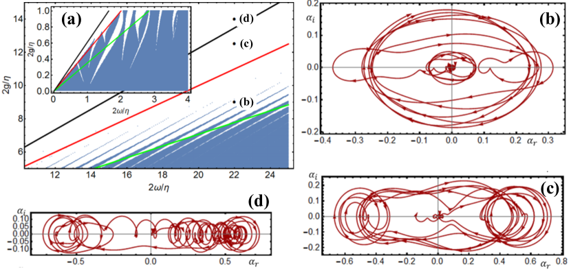
Figure 1: (Color online) (a) Stability diagram in the driving frequency vs. coupling plane, signalling in white the regions with positive instability rate, $\gamma^{*}>0$. The plot is drawn at the static resonance, $\lambda_{0}=1$, with $\lambda=\frac{1}{2}$. The red line marks the static critical coupling $\mu_{0}=1$, while the green one corresponds to $\mu_{min}=1$; so that, for a point under the green line $\mu(t)>1\forall t$, while $\mu(t)$ periodically goes below unity above it. Finally, the black line corresponds to $\mu_{max}=1$. For $g\rightarrow 0$ the white zones open for $\eta_{k}=2\omega_{a}/k$, $k\in Z$. In the limit $\eta\rightarrow\infty$ the first blue triangle on the left tends to fill the whole region under the red line, while for $\eta\rightarrow 0$ it is the region under the green line that becomes blue. The inset shows the stability diagram for larger values of the driving frequency. (b)-(d) Trajectories of the mean field $\alpha$ corresponding to the three points in panel (a). We have assumed a slow periodic driving ($\omega_{a}=11\eta$) and evaluated $\alpha(t)$ up to $t=60\eta^{-1}$ by numerically solving Eqs. (5) for the parameters indicated by the black dots in the central panel, with $2g/\eta=9,12.5,14$. Initially, the radiation field has been taken in the coherent state $|{\sqrt{N}\epsilon}\rangle$ with $\epsilon=10^{-2}$, with all of the atoms in their ground states.

In the following, we focus on a periodically driven system. We specifically assume the atomic frequency to be sinusoidally perturbed, $\omega_{b}/\omega_{a}=\lambda_{0}+\lambda\sin(\eta t)$, as in  Vacanti12PRL108 , implying an harmonic time dependence for $\mu(t)$, which oscillates with frequency $\eta$, between $\mu_{min}=\mu_{0}(1-\lambda/\lambda_{0})$ and $\mu_{max}=\mu_{0}(1+\lambda/\lambda_{0})$, where $\mu_{0}=\lambda_{0}\omega_{a}^{2}/4g^{2}$. For such a periodic driving, we can make use of Floquet theory Floq to study the dynamics of the system. In particular, the stability of the solutions of Eqs. (5) can be characterized by an instability rate $\gamma^{*}$ defined as the largest positive Floquet exponent of the linearized equations Floq , which embodies the growing rate of the mean fields in the linear regime. While the details of this analysis are given in the supplementary material nota , the result is reported in Fig. 1, where we see that $\gamma^{*}>0$ if $\mu(t)<1$ at all times (above the black line in Fig. 1), while driving-induced instabilities appear even in the (static) N region (below the red line in Fig. 1). For small couplings, this occurs near the parametric resonance points $\eta_{k}=\omega_{a}(1+\lambda_{0})/k$ ($k\in\mathbb{Z}$). These are the so called Arnold instability tongues, discussed in Bastidas12PRL108 . Although our treatment is valid in general, the discussion below will mainly focus on the case of a slow (but non-adiabatic) driving, therefore Fig. 1 explicitly displays the case $\eta\ll\omega_{a},\omega_{b}$.

Although the dynamics can exit the linear regime when the mean fields acquire large values (which can occur quite quickly, e.g., for initial coherent states with very small amplitudes), the diagram in Fig. 1 still helps classifying the dynamical behavior of the mean fields, identifying those values of frequency and coupling for which $\alpha$ and $\beta$ grow exponentially in time, from those for which they stay bounded. As shown below, the very same diagram will help in the study of quantum fluctuations (cfr. the discussion after Eq. 6).

Solutions of Eqs. (5) in the different regimes are reported in Fig. 1 (b)-(d), where various examples of trajectories of the photon mean field $\alpha$ are shown ($\beta(t)$ follows similar paths). At $t=0$ the electromagnetic mode is taken in the coherent state $|{\sqrt{N}\epsilon}\rangle$ (with $\epsilon\ll 1$), while the atoms are in their ground states. If the system’s parameters are chosen in the unstable region, the mean fields grow exponentially and, once out of the linear regime, get macroscopic values. For a set of parameters in the stable zone, instead, the trajectory is bounded, with $|\alpha(t)|$ remaining $\sim\epsilon$. This behavior is quite general and does not depend on the value of the driving frequency.

For a slow driving, the trajectories show some regularity as, after an initial amplification stage, the mean fields remarkably tend to be attracted towards the nearest of the equilibrium points; namely, either $(\alpha^{n},\beta^{n})$, or one of the two broken symmetry points $(\alpha^{sr}_{\pm},\beta^{sr}_{\pm})$, which is then ‘followed’ as its value changes due to the driving. More specifically, when $\mu(t)>1$, the two mean fields circulate around their N stationary point, $\alpha^{n}$ and $\beta^{n}$, respectively. A switching occurs once $\mu(t)$ crosses its critical value, with the mean field trajectory that dynamically breaks the parity symmetry, “selects a sign”, and moves towards either the positive or the negative real axis, to begins rotating around one of SR values. When, later, we get $\mu(t)>1$ again, the mean fields are attracted back by the N fixed point, to move again towards one of the SR points further on. Such a sequence of switching events occurs if the driving parameters and the coupling strength are such that $\mu_{0}\in[(1+\lambda/\lambda_{0})^{-1},1]$ whose boundaries correspond to the black and red lines in Fig. 1 (a), respectively. This is the case, e.g., of Fig.  1 (c). A different behavior is found for $\mu_{0}\in(1,(1-\lambda/\lambda_{0})^{-1}]$, where the right boundary corresponds to the green line in Fig. 1 (a). In this case, although $\mu<1$ for some $t$, the trajectory keeps rotating around the N equilibrium point, as in Fig. 1 (b). For parameters taking us below the green line, the driving is not able to bring the system to criticality and the solution of Eqs. (5) never exit the linear regime. Correspondingly, the values of the mean fields remain of order $\epsilon$. Above the black line, on the other hand, only the two SR stationary points come into play. One further particular trajectory for the mean photon field, in the regime in which both the N and the SR points are relevant, is analyzed in detail in Fig. (2), which shows how the field follows the instantaneous equilibrium point, dynamically breaking the equivalence between the two SR values when entering the regime with $\mu<1$.

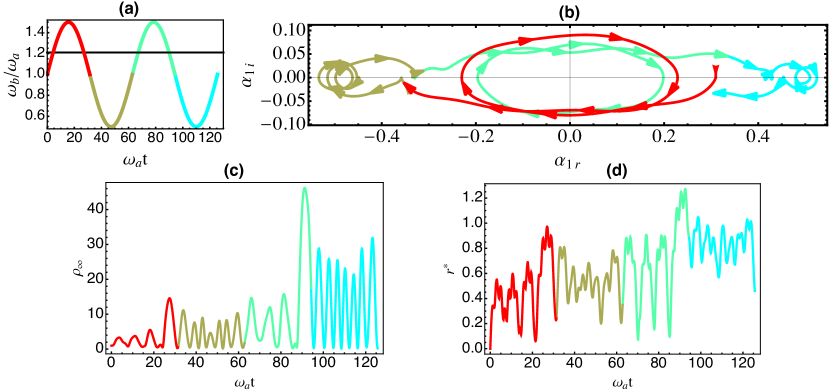
Figure 2: (Color online): We show the driving cycle [panel (a)], the mean field trajectory (b), the photon number fluctuations $\rho_{\infty}$ (c), and the two-mode squeezing parameter $r^{*}$ (d). In panels (b)-(d), segments of a given color refer to the corresponding part of the driving cycle [panel (a)]. We set $\eta=0.1\omega_{a}$ and $\lambda=0.5$, with $\lambda_{0}=1$, and $g=0.55\omega_{a}$. Initial conditions are $\alpha(0)=\alpha^{sr}(0)$ and $\beta(0)=\beta^{sr}(0)$.

The dynamic mean fields are not sufficient to obtain the average value of a generic observable. This is the case, for instance, of the photon number. A complete quantum description requires the knowledge of the (operator) fluctuations around the mean fields. The associated equations of motion for the fluctuations are explicitly derived in nota . They are best displayed in terms of the quadrature vector $\hat{\bm{Q}}(t)=(\hat{q}_{c},\hat{q}_{d},\hat{p}_{c},\hat{p}_{d})$ with $\hat{q}_{k}=(\hat{k}+\hat{k}^{{\dagger}})/\sqrt{2}$, $\hat{p}_{k}=i(\hat{k}^{{\dagger}}-\hat{k})/\sqrt{2}$ ($k=c,d$), and take the form

$$\dot{\hat{\bm{Q}}}(t)={\bm{M}}_{\alpha,\,\beta}\,\hat{\bm{Q}}(t),$$ (6)

where matrix ${\bm{M}}_{\alpha,\,\beta}$ is a non-linear function of the instantaneous mean field values $\alpha$ and $\beta$ nota . Although the dynamics of the mean fields discussed above is independent of the fluctuations, the reverse is not true. Moreover, for $\alpha,\beta\ll 1$ (i.e. when the mean fields are in the linear regime), ${\bm{M}}_{\alpha,\,\beta}$ reduces to the very same dynamical kernel ruling Eqs. (5) for $t<t_{\text{lin}}$. This implies that the stability analysis of Fig. 1 applies to the quantum fluctuations as well. In particular, for a parameter set in the white region, the dynamics of the fluctuations becomes chaotic: two very close initial states exponentially diverge in time, at a rate $\gamma^{*}$. Eq. (6) are formally solved as $\hat{\bm{Q}}(t)=\Phi(t)\hat{\bm{Q}}(0)$, where matrix $\Phi$ is such that $\dot{\Phi}={\bm{M}}_{\alpha,\,\beta}\Phi$ and satisfies the boundary condition $\Phi(0)=\mathds{1}$. The first moments of the quadratures are zero at all times (as the averages are given by the mean fields), while the second moments form the covariance matrix $W$ with elements $W_{i\,j}=\langle\{\hat{Q}_{i},\hat{Q}_{j}\}\rangle/2-\langle\hat{Q}_{i}\rangle\langle\hat{Q}_{j}\rangle$, Weedbrook2012 ; Simon1994 ; Ferraro05arxiv . The time-evolved covariance matrix is then given by $W(t)=\Phi(t)W(0)\Phi(t)^{T}$. In general, both the mean fields and the quantum fluctuations contribute to the evolution of a physical observable, an interesting example being given by the average photon number

$$n_{a}=\langle\hat{a}^{{\dagger}}\hat{a}\rangle\equiv N\left|\alpha\right|^{2}+\left(W_{11}+W_{33}-1\right)/2.$$ (7)

Covariance matrix contributions dominate for initial mean fields values $\lesssim N^{-1/2}$, and, in particular, if one takes the vacuum of both modes as initial state. In fact, in virtue of the previous discussion, this implies $\alpha=\beta=0\,\forall t$, so that photons are generated, in this case, by the exponential amplification of the initial fluctuations, due to the instability of the system under sinusoidal perturbation signalled by a positive instability rate $\gamma^{*}$. For a very fast perturbation, $\eta\gg\omega_{a},\omega_{b}$, this requires $\mu_{0}<1$. On the other hand, if $\mu_{0}>1$, fluctuations are bounded in time. Differently, for a very slow perturbation, photon production occurs if we can make $\mu(t)<1$ in some time interval, while fluctuations are bounded only if $\mu(t)>1\,\forall t$. Photon generation from the vacuum is related to the thermodynamic work done on the system by the driving agent work . The average work performed at time $t$ is

$$\langle w\rangle =\langle\hat{H}\rangle_{t}-\langle\hat{H}\rangle_{0}=\omega_{a}n_{a}(t)+{N}\omega_{b}(0)/2+2gW_{12}(t)$$ (8)

$$+{\omega_{b}(t)}\left[W_{22}(t)+W_{44}(t)-(N+1)\right]/2,$$

which depends not only on the local energies of the two modes involved, but also on their correlations through the $W_{12}$ term. Eq. (8) shows that not all of the energy pumped into the system is used for photon production in light of the non-adiabatic nature of the driving. Part of such energy goes to the atoms and part is stored as interaction energy. The non-adiabaticity of the driving process can be quantitatively studied using specifically designed thermodynamic figures of merit for irreversibility work . Among them is the inner friction Plastina14PRL113 , which is defined as the non-adiabatic part of the work. In our case, assuming the coupling to be switched on at $t=0$, it reads $\langle w_{fric}\rangle=\langle w\rangle-E^{t}_{GS}+E^{0}_{GS}$, where $E^{t}_{GS}$ is instantaneous energy of the ground state $\left|GS\right\rangle$ of the system, which becomes non-analytic for $\mu=1$. The behavior of $\langle w_{fric}\rangle$ crucially depends on the driving amplitude $\lambda$.If $\lambda$ is such that $\mu_{min}>1$,the system never exit the N region and $\langle w_{fric}\rangle$ never gets macroscopic values. If $\mu_{min}=1$(i.e., $\mu=1$ at times $\eta t=(3/2+2k)\pi$, $k\in\mathbb{Z}^{*}$), the inner friction becomes non analytic (as the energy gap closes), yet remaining ${\cal O}(1)$ as $N\rightarrow\infty$. If $\lambda$ is such that $\mu_{min}<1$,instead, the system enters the SR region for $t\in[(2k-1)\pi+\tilde{t},2k\pi-\tilde{t}]$, where $\eta\tilde{t}=\arcsin(\lambda_{c}/\lambda)$ ($k\in\mathbb{Z}^{*}$). Then, as the evolved state becomes macroscopically different from the instantaneous ground state, inner friction gets macroscopic values. Altogether, the inner friction per atom in the thermodynamic limit is

$$\lim_{N\rightarrow\infty}{\langle w_{fric}\rangle}/{N}=\begin{cases}0&\text{for}\leavevmode\nobreak\ \mu(t)\geq 1,\\ {\omega_{b}(t)}[1-1/\mu(t)]^{2}/4&\text{for}\leavevmode\nobreak\ \mu(t)<1.\end{cases}$$ (9)

Besides the mean photon number and the average (non-adiabatic) work, we can characterize the photon statistics by the variance, $\sigma_{a}^{2}=\langle(a^{\dagger}a)^{2}\rangle-n_{a}^{2}$, and the Mandel parameter $\rho=\frac{\sigma_{a}^{2}}{n_{a}}$. The latter signals a sub- or super-Poissonian statistics, with $\rho=1$ for a coherent state. For very large $N$, in the regime in which the mean fields dominate with respect to quantum fluctuations (which is the case for initial mean fields larger than $N^{-1/2}$), and neglecting ${\cal O}(\sqrt{N})$ terms, the variance is

$$\sigma_{a}^{2}=2N\left(\alpha_{r}^{2}W_{11}+\alpha_{i}^{2}W_{33}+2\alpha_{r}\alpha_{i}W_{13}\right)$$ (10)

so that, as $N\rightarrow\infty$, the Mandel parameter becomes

$$\rho_{\infty}={2}(\alpha_{r}^{2}W_{11}+\alpha_{i}^{2}W_{33}+2\alpha_{r}\alpha_{i}W_{13})/|\alpha|^{2}$$ (11)

In general terms, the time behavior of the quantum fluctuations is very different depending on wether $\mu$ is larger or smaller than $1$. This is reflected in the covariance matrix and witnessed by the parameter $\rho_{\infty}$ (see Fig. 2). Roughly, this is an oscillating function of time, which oscillates faster as the mean fields get larger, with an amplitude that suddenly increases whenever $\mu$ crosses $\mu_{c}$ to enter in the SR region.

While $n_{a}$ and $\rho$ describe the reduced photon-state only, we can also characterize global state correlations by evaluating the degree of two-mode squeezing. With this aim, we consider the parameter $r_{opt}(t)$ optimizing the fidelity Marian12PRA86 between $\left|\psi,t\right\rangle$ and the two-mode squeezed coherent state $\left|\psi_{\alpha,\,\beta}(r,t)\right\rangle$ having coherent amplitudes given by the mean fields and (real) squeezing degree $r$, i.e. $|{\psi_{\alpha,\beta}(r,t)}\rangle=e^{r(c^{\dagger}d^{\dagger}-cd)}\left|\sqrt{N}\,\alpha(t)\right\rangle_{a}\left|\sqrt{N}\,\beta(t)\right\rangle_{b}$. Regardless of $t$, we find a value $r_{opt}(t)$ for which the fidelity is $\geq 0.9999$ nota . Therefore, $r_{opt}$ itself can be thought as a good (although approximate) descriptor of the photon-atom entanglement, Horodecki96PLA96 ; Simon00PRL84 . During time evolution, it turns out that $r_{opt}$ can either grow exponentially at short times (if $\gamma^{*}>0$), or remains very close to its initial value (for $\gamma^{*}=0$). An example of the behavior of $r_{opt}$ is reported in Fig. (2), for the various stages of the driving induced dynamics. After the initial fast increase, $r_{opt}$ displays small ‘jumps’ whenever the driving brings the system in the SR region.

Concluding remarks.-We have provided a dynamical mean field-based description of the driven Dicke model, discussing the non-linear evolution of the mean fields, as well as that of quantum fluctuations. Both are needed to determine the time behavior of physical observables such as the photon number. Our approach is exact in the thermodynamic limit. However, for finite $N$, our description is accurate provided that fluctuations do not become macroscopic (otherwise the expansion in Eq. (4) breaks down). This gives a time limit $t_{max}$ (generically increasing with $N$) within which the analysis is meaningful. Remarkably $t_{max}$, which is estimated in nota , may be different in the various dynamical regimes. Within such limit, we have discussed the phenomenon of dynamical breaking of the parity symmetry in the mean field evolution under driving, analysed photon generation from the vacuum, using out-of-equilibrium thermodynamical tools to characterize it, and described the generation of two-mode squeezing and entanglement between field and atoms.

Acknowledgements We acknowledge support from the Collaborative Projects QuProCS (Grant Agreement 641277), and TherMiQ (Grant Agreement 618074), the John Templeton Foundation (grant number 43467), the Julian Schwinger Foundation (grant number JSF-14-7-0000), and the UK EPSRC (grant number EP/M003019/1). We acknowledge partial support from COST Action MP1209.

I Supplementary material

I.1 Holstein-Primakoff trasformation

Since the total spin $|\vec{J}|^{2}$ is conserved, the full Hilbert space can be decomposed into invariant subspaces labelled by the index $j$ describing its eigenvalues, $j=1,2,\cdots,\frac{N}{2}$ for an even $N$, or $j=\frac{1}{2},\cdots,\frac{N}{2}$ if $N$ is odd. Defining the projector $P_{j}$ onto $j$-th subspace, we can rewrite the Hamiltonian as $H=\sum_{j}P_{j}HP_{j}\equiv\sum_{j}H^{(j)}$

In the main text we focus on the case of a fully symmetric initial atomic state, which implies selecting the $j=\frac{N}{2}$ invariant subspace. We therefore performed the Holstein-Primakoff transformation on the spin operators projected in this sector alone. The procedure, however, could have been repeated for each $j$. To start with, one has to express the projected spin $\vec{J}^{(j)}=P_{j}\vec{J}P_{j}$ through boson operators $b_{j},b_{j}^{{\dagger}}$:

$$J_{z}^{(j)}=b_{j}^{\dagger}b_{j}-j\,,\quad J_{+}^{(j)}=b_{j}^{\dagger}\sqrt{2j-b_{j}^{\dagger}b_{j}}$$

so that the projected Hamiltonian is

$$H^{(j)} = \omega_{a}a^{\dagger}a+\omega_{b}\left(b_{j}^{\dagger}b_{j}-j\right)+$$

$$g\left(a^{\dagger}+a\right)\left(b_{j}^{\dagger}\sqrt{1-2\frac{b_{j}^{\dagger}b_{j}}{j}}+\sqrt{1-2\frac{b_{j}^{\dagger}b_{j}}{j}}b_{j}\right)$$

In the main text, $j=N/2$ is taken and all of the subscripts are erased.

I.2 Equations of motion

The core of our approximate analysis is the expansion of the non linear term

$$\sqrt{1-\frac{b^{\dagger}b}{N}}=\sqrt{\Gamma}\sqrt{1-\frac{\sqrt{N}(\beta d^{\dagger}+\beta^{*}d)+d^{\dagger}d}{N}}\,.$$ (13)

In the limit $N\rightarrow\infty$, this can be expanded into a power series as

$$\sqrt{1-\frac{b^{\dagger}b}{N}} = \sqrt{\Gamma}\bigg{(}1-\frac{\beta d^{\dagger}+\beta^{*}d}{2\sqrt{N}\Gamma}-\frac{d^{\dagger}d}{2N\Gamma}$$

$$-\frac{\left(\beta d^{\dagger}+\beta^{*}d\right)^{2}}{8N\Gamma^{2}}\bigg{)}+O\left(N^{-\frac{3}{2}}\right)$$

with $\alpha(t)$ and $\beta(t)$ assumed to stay order $O(1)$ so that the lowest order term gives already a good approximation once inserted in the Hamiltonian.

Using the leading contribution only, the Hamiltonian becomes

$$H^{(N/2)} = \omega_{a}c^{\dagger}c+\left[\omega_{b}-2g\frac{\alpha_{r}\beta_{r}}{\sqrt{\Gamma}}\left(2+\frac{|\beta|^{2}}{2\Gamma}\right)\right]d^{{\dagger}}d+$$ (15)

$$g\sqrt{\Gamma}(c^{\dagger}+c)\left[\left(1-\frac{\beta^{*}\beta_{r}}{\Gamma}\right)d+h.c.\right]-$$

$$g\frac{\alpha_{r}}{\sqrt{\Gamma}}\left[\beta^{*}\left(1+\frac{\beta^{*}\beta_{r}}{2\Gamma}\right)d^{2}+h.c.\right]+$$

$$\sqrt{N}\left(\Delta_{c}^{*}c+\Delta_{d}^{*}d+h.c.\right)+\Lambda_{N}+O\left(\frac{1}{\sqrt{N}}\right)$$

where we defined $\Delta_{c}$ and $\Delta_{d}$ as

$$\vec{\Delta}=\left(\begin{array}[]{c}\Delta_{c}\\ \Delta_{d}\\ \end{array}\right)=\left(\begin{array}[]{c}\omega_{a}\alpha+2g\sqrt{\Gamma}\beta_{r}\\ \omega_{b}\beta+2g\sqrt{\Gamma}\alpha_{r}\left(1-\frac{\beta\beta_{r}}{\Gamma}\right)\\ \end{array}\right)$$ (16)

while $\Lambda_{N}$ is the c-number

$$\Lambda_{N} = N\left\{\omega_{a}|\alpha|^{2}+\omega_{b}\left(|\beta|^{2}-\frac{1}{2}\right)+4g\sqrt{\Gamma}\alpha_{r}\beta_{r}\right\}-$$ (17)

$$g\alpha_{r}\beta_{r}\frac{|\beta|^{2}}{2\sqrt{\Gamma}}$$

In the strict thermodynamic limit, thus, the Hamiltonian becomes quadratic, so that the time evolution can be described by a Gaussian propagator.

We describe the dynamics in the Heisenberg picture, and obtain the following equation for the annihilation operators:

$$i\frac{d}{dt}c^{(H)}(t) = -U^{\dagger}(t,0)\left[H^{(N/2)}(t),c\right]U(t,0)-i\sqrt{N}\frac{d\alpha(t)}{dt}$$

$$= \omega_{a}c^{(H)}+g\sqrt{\Gamma}\left[\left(1-\frac{\beta^{*}\beta_{r}}{\Gamma}\right)d^{(H)}+h.c.\right]$$

$$+\sqrt{N}\Delta_{c}-i\sqrt{N}\frac{d\alpha}{dt}+O\left(\frac{1}{\sqrt{N}}\right)$$

In order for the operator $c$ to stay of order $O(1)$, the two terms $\sim\sqrt{N}$ above should compensate each other. To this end, we require the mean field $\alpha$ to satisfy

$$i\frac{d\alpha}{dt}=\Delta_{c}$$ (19)

In this way, the Heisenberg equation becomes

$$i\frac{d}{dt}c^{(H)}=\omega_{a}c^{(H)}+g\sqrt{\Gamma}\left[\left(1-\frac{\beta^{*}\beta_{r}}{\Gamma}\right)d^{(H)}+h.c.\right]+O\left(\frac{1}{\sqrt{N}}\right)$$ (20)

In the limit $N\rightarrow\infty$ the terms $O\left(\frac{1}{\sqrt{N}}\right)$ do not bring any contribution to the dynamics of the operator $c^{(H)}$. For finite $N$, on the other hand, in order to give a more accurate description of the dynamics of the fluctuations, one should consider further terms in the expansion (I.2). Even if this is done, however, the dynamics of the mean field will remain unchanged, as it is determined by the $\sim\sqrt{N}$ terms only.

After a similar analysis is carried out for the operator $d$, we find the differential equation for $\beta$

$$i\frac{d\beta}{dt}=\Delta_{d}$$ (21)

and the Heisenberg equations

$$i\frac{d}{dt}d^{(H)} = \left(\omega_{b}-2g\frac{\alpha_{r}\beta_{r}}{\sqrt{\Gamma}}\left(2+\frac{|\beta|^{2}}{2\Gamma}\right)\right)d^{(H)}$$ (22)

$$+g\sqrt{\Gamma}\left(1-\frac{\beta\beta_{r}}{\Gamma}\right)(c^{(H)}+h.c.)$$

$$-2g\frac{\alpha_{r}\beta}{\sqrt{\Gamma}}\left(1+\frac{\beta\beta_{r}}{2\Gamma}\right){d^{(H)}}^{\dagger}+O\left(\frac{1}{\sqrt{N}}\right)$$

I.3 Time evolution of the mean fields

Explicitly, the equations for the real and imaginary parts of the re-scaled mean fields are

$$\begin{cases}\dot{\alpha}_{r}=\omega_{a}\alpha_{i}\\ \dot{\alpha}_{i}=-\omega_{a}\alpha_{r}-2g\sqrt{\Gamma}\beta_{r}\\ \dot{\beta}_{r}=\omega_{b}\beta_{i}-2g\alpha_{r}\frac{\beta_{r}\beta_{i}}{\sqrt{\Gamma}}\\ \dot{\beta}_{i}=-\omega_{b}\beta_{r}-2g\sqrt{\Gamma}\alpha_{r}(1-\frac{\beta_{r}^{2}}{\Gamma})\end{cases}$$ (23)

If we regard $\alpha_{r}$ and $\beta_{r}$ as the generalized coordinates, and $\alpha_{i}$ and $\beta_{i}$ as their conjugate momenta, these equations can be derived from the Hamiltonian function

$$H(\alpha,\beta)=\frac{\omega_{a}}{2}|\alpha|^{2}+\frac{\omega_{b}}{2}|\beta|^{2}+2g\sqrt{\Gamma}\beta_{r}\alpha_{r}$$

They can be considered as purely classical equations, but should be solved with initial conditions that comes from the choice of an initial quantum state:

$$\left(\begin{array}[]{c}\alpha(0)\\ \beta(0)\\ \end{array}\right)=\frac{1}{\sqrt{N}}\left(\begin{array}[]{c}\langle a(0)\rangle\\ \langle b(0)\rangle\\ \end{array}\right)$$ (24)

As our treatment is based on the requirement that fluctuations stay of lower order than averages, we need to restrict our-selves to initial quantum states that fulfill this very same condition.

The system (23) can be linearized if the initial conditions are such that $|\alpha(0)|,|\beta(0)|\ll 1$. Then, until the time $t_{lin}$ such that $\alpha$ and $\beta$ are of order one, the dynamics of the mean fields can be described by the linearized system

$$\frac{d}{dt}\left(\begin{array}[]{c}\alpha_{r}\\ \beta_{r}\\ \alpha_{i}\\ \beta_{i}\\ \end{array}\right)\approx M_{0}\left(\begin{array}[]{c}\alpha_{r}\\ \beta_{r}\\ \alpha_{i}\\ \beta_{i}\\ \end{array}\right)$$ (25)

where

$$M_{0}=\left(\begin{array}[]{cccc}0&0&\omega_{a}&0\\ 0&0&0&\omega_{b}\\ -\omega_{a}&-2g&0&0\\ -2g&-\omega_{b}&0&0\\ \end{array}\right)$$

I.4 Time evolution of the fluctuations

As for the quantum fluctuations, we can recast the Heisenberg equations (20) and (22) in a more compact form using the quadrature operators $\vec{Q}=(q_{c},q_{d},p_{c},p_{d})$ as introduced in the main text. In the limit $N\rightarrow\infty$, we find

$$\dot{\vec{Q}}^{(H)}=M_{\alpha,\beta}\vec{Q}^{(H)}$$

where $M_{\alpha,\beta}$ is the matrix

$$M_{\alpha,\beta}=\left(\begin{array}[]{cccc}0&0&\omega_{a}&0\\ -\frac{2g\beta_{r}\beta_{i}}{\sqrt{\Gamma}}&-\frac{2g\alpha_{r}\beta_{i}}{\sqrt{\Gamma}}\left(1+\frac{\beta_{r}^{2}}{\Gamma}\right)&0&\omega_{b}-\frac{2g\alpha_{r}\beta_{r}}{\sqrt{\Gamma}}\left(1+\frac{\beta_{i}^{2}}{\Gamma}\right)\\ -\omega_{a}&-2g\sqrt{\Gamma}\left(1-\frac{\beta_{r}^{2}}{\Gamma}\right)&0&2g\frac{\beta_{r}\beta_{i}}{\sqrt{\Gamma}}\\ -2g\sqrt{\Gamma}\left(1-\frac{\beta_{r}^{2}}{\Gamma}\right)&-\omega_{b}+\frac{2g\alpha_{r}\beta_{r}}{\sqrt{\Gamma}}\left(3+\frac{\beta_{r}^{2}}{\Gamma}\right)&0&\frac{2g\alpha_{r}\beta_{i}}{\sqrt{\Gamma}}\left(1+\frac{\beta_{r}^{2}}{\Gamma}\right)\\ \end{array}\right)$$ (26)

We can define the fundamental matrix $\Phi$ as the solution of the differential equation

$$\dot{\Phi}=M_{\alpha,\beta}\Phi$$ (27)

with the initial condition $\Phi(0)=\mathds{1}$. Then the solution of the Heisenberg equation is

$$\vec{Q}^{(H)}(t)=\Phi(t)\vec{Q}$$

In our description the first moments are zero for every time, i.e. $\langle\vec{Q}\rangle=\vec{0}$. The second moments are given by the covariance matrix $W$, as mentioned in the main text. If the initial state is Gaussian, then the covariance matrix completely characterizes the fluctuations around the mean fields.

In the linear transient regime, $t<t_{lin}$, we find that $M_{\alpha,\beta}=M_{0}$, so that the dynamics of the fluctuations are the same as the mean field ones. Furthermore, if the initial state is such that $\alpha(0)=\beta(0)=0$, then the mean fields will remain zero $\forall t$ and, thus the dynamics of the fluctuations is described by $M_{0}$ at all times.

In general, $M_{\alpha,\beta}$ has a parametric time dependence, as it contains $\omega_{b}(t)$. Therefore, it inherits from $\omega_{b}$ a periodicity of $T=2\pi/\eta$. Then, by the Floquet theorem, we can write

$$\Phi(t)=e^{-\frac{Bt}{T}}\,P(t)\,,$$

with a constant $B$ and a periodic $P(t)$. For us, $\Phi(0)=\mathds{1}$, therefore also $P(0)=P(T)=\mathds{1}$. As a result, we have that the so called monodromy matrix is $\Phi(T)=e^{-B}$.

I.5 Limits of validity for finite $N$

Our description of the dynamics becomes exact for every finite time $t$ in the limit $N\rightarrow\infty$. Anyway, it’s crucial to understand what the limits of applicability of our approach are for finite $N$. We observe that, during the time evolution, fluctuations (assumed to be $O(1)$ at $t=0$) can become very large and even unbounded. When this happens, the expansion of the square root in the Hamiltonian may become incorrect. In other words, for finite but large $N$ our description stays accurate until the n-th moments become of order $N^{n/2}$. To ensure that this is not the case, it is enough to require that all of the elements of the matrix $\Phi$ are small compared to $\sqrt{N}$. Therefore, our description of the dynamics is accurate until a time $t_{max}$, defined as the first instant for which

$$max_{i\,j}\left\{\Phi_{ij}(t_{max})\right\}\approx\sqrt{N}$$ (28)

In the limit $N\rightarrow\infty$, we expect $t_{max}\rightarrow\infty$.

In order to characterize and estimate $t_{max}$, we need to consider the initial conditions for the mean fields, $\alpha(0)=\alpha_{0}$ and $\beta(0)=\beta_{0}$. In particular, if we take $\delta=max\left\{|\alpha_{0}|,|\beta_{0}|\right\}\ll 1$, the first part of the dynamics is included in the linear transient. This implies that, for $0\leq t<t_{lin}$, the time evolution of both the fluctuations and of the mean-fields is determined by the linearized matrix $M_{0}$.

In the absence of driving and in the linear transient, the dynamics would be characterized by the eigenvalues of the matrix $M_{0}$. Two of them are always purely imaginary, i.e. $\pm i\lambda_{1}$. The other two are $\pm i\lambda_{2}$, where $\lambda_{2}$ is real if $\mu>1$, it is equal to $\lambda_{1}$ if $\mu=1$ and it is purely imaginary if $\mu<1$. This means that if $\mu>1$ the fluctuations and the mean fields stay always of the same order, i.e $t_{lin}\rightarrow\infty$ and $t_{max}\rightarrow\infty$. At the transition point, $\mu=1$, fluctuations and mean-fields grow linearly in time; while in the super-radiant phase $\mu<1$, the fluctuations and the mean fields can experience an exponential growth, with an instability rate given by $\gamma^{*}=|\lambda_{2}|$. This is true until $t\lesssim t_{lin}$. After $t_{lin}$, the nonlinear terms cannot be neglected anymore and one has to consider the full non-linear equations. Thus, within the linear regime, we can define the characteristic time $\tau^{*}$ as the inverse of the instability rate, i.e.

$${\tau^{*}}^{-1}=\gamma^{*}=\sqrt{\sqrt{\left(\frac{\omega_{a}^{2}-\omega_{b}^{2}}{2}\right)^{2}+4\omega_{a}\omega_{b}g^{2}}-\frac{\omega_{a}^{2}+\omega_{b}^{2}}{2}}$$

We can estimate $t_{lin}$ as the time for which one of the mean fields (either $\alpha$ or $\beta$) becomes of order one,

$$t_{lin}\approx\tau^{*}\ln\left(\delta^{-1}\right)$$ (29)

Since $\delta\ll 1$, we expect $t_{lin}$ to be much larger than $\tau^{*}$. The crucial point, however, is wether or not all of the linear transient is contained within our limit of validity. Indeed, for this description to be valid for times of the order of $t_{lin}$, we have to require that

$$e^{\gamma^{*}t_{lin}}\ll\sqrt{N}$$

from which it follows that

$$t_{lin}\ll\frac{\tau^{*}}{2}\ln(N)$$

and that

$$\delta\gg\frac{1}{\sqrt{N}}$$

This means that if the initial state is not so close to the vacuum (the difference from zero of $\alpha$ and $\beta$ being larger than $\frac{1}{\sqrt{N}}$), then $t_{lin}\ll t_{max}$. In this case, our description makes full sense even outside the linear transient, and can be used even when the mean-fields take macroscopic values. In this case, $t_{lin}$ can indeed be estimated by (29) and is finite. On the other hand, for finite $N$, it is not possible to give a simple expression for $t_{max}$, as it depends on the non-linear terms appearing in the time evolution, and the only way to check the validity of our approach is to check the condition (28).

Instead, if both of the mean fields start too close to zero, specifically if $\delta\lesssim\frac{1}{\sqrt{N}}$, then our description ceases to be good before the mean fields $\alpha$ and $\beta$ reach macroscopic values. In this case, in fact, $t_{max}$ is inside the linear transient, and, from (28), we can make the simple estimate

$$t_{max}=\frac{\tau^{*}}{2}\ln(N)$$

These estimates and reasoning can be adapted also to the case of a driven system, since they are simply a consequence of the fact that the dynamics of the mean fields and that of the fluctuations are the same in the linear transient.

For instance, for a periodically driven Hamiltonian, we can use the largest positive Floquet exponent of the linearized matrix $M_{0}$ in order to estimate $\tau^{*}$; and then use again the equations above to estimate $t_{lin}$ and $t_{max}$. Specifically, if $M_{0}$ is periodic in time, with period $T$, then the monodromy matrix (in the Floquet description) is given by $\mathcal{M}=\Phi(T)$. The eigenvalues of $\mathcal{M}$ are the Floquet multipliers $\{\rho_{i}\}_{i=1}^{4}$. From these, we can calculate the Floquet exponents, that are the complex numbers $\nu_{i}=\frac{\ln(\rho_{i})}{T}$. So we can define the instability rate $\gamma^{*}$ as the maximum among zero and the real parts of the Floquet exponents, i.e.

$$\gamma^{*}=max\left\{0,\,\left\{\mathds{R}e\{\nu_{i}\}\right\}_{i=1}^{4}\right\}$$ (30)

As a result, the arguments above can be applied in this case too, even if, in a strict sense, the stability of the dynamics cannot be fully characterized by the instantaneous eigenvalues of the matrix $M_{0}$.

I.6 Optimal degree of two-mode squeezing

As discussed in the main text, we compare the instantaneous state of the global (atom+field) system with the two-mode squeezed coherent state $\left|\psi_{\alpha,\beta}(r,t)\right\rangle$ obtained by applying the unitary squeeze operator of (real) degree $r$,

$$S(r)=e^{r(c^{\dagger}d^{\dagger}-cd)}\,,$$

to the two-mode coherent state obtained by taking the instantaneous mean fields $\alpha(t)$ and $\beta(t)$ as amplitudes,

$$\left|\psi_{\alpha,\beta}(r,t)\right\rangle=S(r)\left|\sqrt{N}\,\alpha(t)\right\rangle_{a}\left|\sqrt{N}\,\beta(t)\right\rangle_{b}$$ (31)

The fidelity that we obtain by optimizing the parameter $r$, is very close to unity, as reported in Fig. (3).

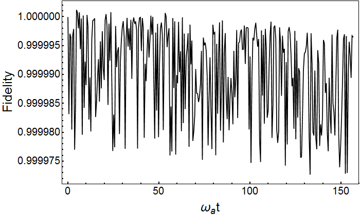
Figure 3: The fidelity $F(t)=|\left\langle\psi_{\alpha(t),\beta(t)}(r_{opt},t)|\Psi,t\right\rangle|^{2}$, evaluated for the same parameter values used in Fig. 2 of the main text. $F(t)$ stays very close to one, tending to slowly decrease for long times.

References

- (1) A. Polkovnikov, K. Sengupta, A. Silva, and M. Vengalattore, Rev. Mod. Phys. 83, 863 (2011).
- (2) J. Eisert, M. Friesdorf, and C. Gogolin, Nat. Phys. 11, 124 (2015).
- (3) B. Damski, Phys. Rev. Lett. 95, 035701 (2005) ; W. H. Zurek, U. Dorner, and P. Zoller, Phys. Rev. Lett. 95, 105701 (2005); J. Dziarmaga, Phys. Rev. Lett. 95 , 245701 (2005); B. Damski and W. H. Zurek, New J. Phys. 10 , 045023 (2008); J. Dziarmaga, Adv. Phys. 59, 1063 (2010); C. De Grandi, V. Gritsev, and A. Polkovnikov, Phys. Rev. B 81, 012303 (2010); P. Silvi, G. Morigi, T. Calarco, S. Montangero Phys. Rev. Lett. 116, 225701 (2016).
- (4) K. Baumann, C. Guerlin, F. Brennecke, and T. Esslinger, Nature (London) 464, 1301 (2010).
- (5) J. Klinder, H. Keßler, M. Wolke, L. Mathey, A. Hemmerich, Proc. Nat. Ac. Sc. 112, 3290 (2015).
- (6) R. H. Dicke, Phys. Rev. 93, 99 (1954); K. Hepp and E. H. Lieb, Ann. Phys. (N.Y.) 76, 360 (1973); Y. Wang and F. Hioe, Phys. Rev. A 7, 831 (1973); C. Emary and T. Brandes, Phys. Rev. Lett. 90, 044101 (2003); T. Brandes, Phys. Rep. 408, 315 (2005); J. Vidal and S. Dusuel, Europhys. Lett. 74, 817 (2006); F. Plastina, G. Liberti, and A. Carollo, Europhys. Lett. 76, 182 (2006); G. Liberti, F. Plastina, and F. Piperno, Phys. Rev. A 74, 022324 (2006); Q. H. Chen, Y. Y. Zhang, T. Liu, and K. L. Wang, Phys. Rev. A 78, 051801(R) (2008); G. Liberti, F. Piperno, F. Plastina, Phys. Rev. A 81, 013818 (2010).
- (7) J. Gong, L. Morales-Molina, and P. Hänggi, Phys. Rev. Lett. 103, 133002 (2009); A. Eckardt, C. Weiss, and M. Holthaus, Phys. Rev. Lett. 95, 260404 (2005). H. Lignier, C. Sias, D. Ciampini, Y. Singh, A. Zenesini, O. Morsch, and E. Arimondo, Phys. Rev. Lett. 99, 220403 (2007); G. Günter et al., Nature (London) 458, 178 (2009).
- (8) V. M. Bastidas, C. Emary, B. Regler, and T. Brandes, Phys. Rev. Lett 108, 043003 (2012).
- (9) M.-J. Hwang, R. Puebla, and M. B. Plenio, Phys. Rev. Lett. 115, 180404 (2015).
- (10) C. Emary, and T. Brandes, Phys. Rev. E 67, 066203, (2003).
- (11) Supplementary Material.
- (12) G. Vacanti, S. Pugnetti, N. Didier, M. Paternostro, G. M. Palma, R. Fazio,V. Vedral, Phys. Rev. Lett. 108, 093603 (2012).
- (13) J. H. Shirley, Phys. Rev. 138, B979 (1965).
- (14) K. Husimi, Miscellanea in Elementary Quantum Mechanics II, Prog. Theor. Phys. 9, 381, (1953).
- (15) C. Weedbrook, and S. Pirandola, Rev. Mod. Phys. 84, 621 (2012).
- (16) R. Simon, N. Mukunda, and B. Dutta, Phys. Rev. A, 49, 1567 (1994).
- (17) A. Ferraro, S. Olivares, and M. G. A. Paris, Gaussian states in continuos variable quantum information, Bibliopolis (Napoli, 2005). (2005).
- (18) M. Campisi, P. Hänggi, and P. Talkner, Rev. Mod. Phys. 83, 771 (2011).
- (19) R. Kosloff and T. Feldmann, Phys. Rev. E 61, 4774 (2000); F. Plastina, A. Alecce, T. J. G. Apollaro, G. Falcone, G. Francica, F. Galve, N. Lo Gullo, and R. Zambrini, Phys. Rev. Lett. 113, 260601 (2014).
- (20) P. Marian and T. A. Marian, Phys. Rev. A, 86, 022340 (2012).
- (21) M. Horodecki, P. Horodecki, and R. Horodecki, Phys. Lett. A, 96, 9601 (1996).
- (22) R. Simon, Phys. Rev. Lett. 84, 2726 (2000)