Random self-similar trees and
a hierarchical branching process

Abstract.

We study self-similarity in random binary rooted trees. In a well-understood case of Galton-Watson trees, a distribution on a space of trees is said to be self-similar if it is invariant with respect to the operation of pruning, which cuts the tree leaves. This only happens for the critical Galton-Watson tree (a constant process progeny), which also exhibits other special symmetries. We extend the prune-invariance setup to arbitrary binary trees with edge lengths. In this general case the class of self-similar processes becomes much richer and covers a variety of practically important situations. The main result is construction of the hierarchical branching processes that satisfy various self-similarity definitions (including mean self-similarity and self-similarity in edge-lengths) depending on the process parameters. Taking the limit of averaged stochastic dynamics, as the number of trajectories increases, we obtain a deterministic system of differential equations that describes the process evolution. This system is used to establish a phase transition that separates fading and explosive behavior of the average process progeny. We describe a class of critical Tokunaga processes that happen at the phase transition boundary. They enjoy multiple additional symmetries and include the celebrated critical binary Galton-Watson tree with independent exponential edge length as a special case. Finally, we discuss a duality between trees and continuous functions, and introduce a class of extreme-invariant processes, constructed as the Harris paths of a self-similar hierarchical branching process, whose local minima has the same (linearly scaled) distribution as the original process.

1. Introduction

Nature commonly exhibits dendritic structures, both static and dynamic, that can be represented by tree graphs [1, 27, 19]. Examples from diverse applications, together with a review of related coalescence and branching models can be found in Aldous [1], Berestycki [2], Bertoin [3], Evans [8], Le Gall [16], and Pitman [21]. Despite their apparent diversity, a number of rigorously studied dendritic structures possess structural self-similarity, which often allows a low-dimensional parameterization [20, 19, 26, 11]. An illuminating example is the combinatorial structure of river networks, which is closely approximated by a two-parametric Tokunaga self-similar model with parameters that are independent of river’s geographic location [25, 20, 6, 29]. Tree self-similarity has been studied primarily in terms of the average values of selected branch statistics, and rigorous results have been obtained only for a very special classes of Markov trees (e.g., binary Galton-Watson trees with no edge lengths, as in [4]). At the same time, solid empirical evidence motivates a search for a flexible class of self-similar models that would encompass a variety of observed combinatorial and metric structures and rules of tree growth. We introduce here a general concept of self-similarity that accounts for both combinatorial and metric tree structure (Sec. 3.5, Def. 12) and describe a model (Sect. 5), called hierarchical branching process, that generates a broad range of self-similar trees (Thm. 4) and includes the critical binary Galton-Watson tree with exponential edge lengths as a special case (Thm. 8). We study time-invariant tree distributions, which is a convenient generalization of Markov growth (Thm. 7). We also introduce a class of critical self-similar Tokunaga processes (Sect. 5.7) that enjoy additional symmetries — their edge lengths are i.i.d. random variables (Prop. 9), and subtrees of large Tokunaga trees reproduce the probabilistic structure of the entire random tree space (Props. 11). The duality between planar trees and continuous functions [9, 21, 28] allows us using the hierarchical branching process to construct a novel class of time series that satisfy the extreme-invariance property: the distribution of their local minima is the same as that of the original series (Sect. 4).

The paper is organized as follows. Section 2 introduces the main definitions, including the Horton-Strahler order of a tree, tree pruning, and a related concept of prune-invariance. Self-similarity for trees with edge lengths is defined in Sect. 3. The duality between trees and continuous functions is reviewed in Sect. 4. In particular, we define here extreme-invariant processes that are equivalent to self-similar trees. The main results are presented in Sect. 5. Sect. 5.1 introduces a hierarchical branching process that generates a rich collection of self-similar trees. The hydrodynamic limit for dynamics of the average numbers of Horton-Strahler branches is established in Sect. 5.2. The properties of criticality and time-invariance are defined in Sect. 5.3 and explored in a self-similar processes in Sect. 5.4. Critical Galton-Watson process and critical Tokunaga processes, which generate the most intriguing examples of self-similar trees, are discussed in Sects. 5.6, 5.7. Section 6 discusses the combinatorial structure of the critical Tokunaga process. Section 7 concludes with two open problems.

2. Random Trees

The focus of this paper is on finite unlabeled rooted reduced planted binary trees with no planar embedding. The space of such trees, which includes the empty tree $\phi$ comprised of a single root vertex and no edges, is denoted by ${\mathcal{T}}$.

The existence of the root vertex imposes the parent-offspring relationship between each pair of the connected vertices in a tree $T\in{\mathcal{T}}$: the one closest to the root is called parent, and the other – offspring. The absence of planar embedding in this context means the absence of order between the two offspring of the same parent. A tree is called reduced if it has no vertices of degree 2; such trees are also called full binary trees. A tree is called planted if its root has degree 1. Accordingly, there are three types of vertices in a tree from ${\mathcal{T}}\setminus\{\phi\}$: internal vertices of degree 3, leaves (degree 1) and the root (degree 1). The operation of series reduction removes each degree-two vertex of a binary tree by merging its adjacent edges into one. Series reduction turns a rooted binary tree into a reduced rooted binary tree. The edges of a tree from ${\mathcal{T}}$ may be assigned positive lengths. The space of trees from ${\mathcal{T}}$ with edge lengths is denoted by ${\mathcal{L}}$.

Any tree from ${\mathcal{T}}$ or ${\mathcal{L}}$ can be embedded (and represented graphically) in a plane by selecting an order for each pair of offspring of the same parent. The space of embedded trees from ${\mathcal{T}}$ (and respectively ${\mathcal{L}}$) is denoted ${\mathcal{T}}_{\rm plane}$ (and respectively ${\mathcal{L}}_{\rm plane}$). Examples of trees from ${\mathcal{L}}_{\rm plane}$ are found in the bottom row of Fig. 1. Choosing different embeddings for the same tree $T\in{\mathcal{T}}$ (or $T\in{\mathcal{L}}$) leads, in general, to different trees from ${\mathcal{T}}_{\rm plane}$ (or ${\mathcal{L}}_{\rm plane}$). Sometimes we focus on the combinatorial tree ${\textsc{shape}(T)}\in{\mathcal{T}}$, which retains the branching structure of $T$ while omitting its edge lengths and embedding.

2.1. Tree pruning and related concepts

The concept of self-similarity is related to the pruning operation [20, 4, 11]. Pruning (aka Horton pruning) of a tree is an onto function ${\mathcal{R}}:{\mathcal{T}}\to{\mathcal{T}}$, whose value ${\mathcal{R}}(T)$ for a tree $T\neq\phi$ is obtained by removing the leaves and their parental edges from $T$, followed by series reduction. We also set ${\mathcal{R}}(\phi)=\phi$.

The pruning is also well defined for trees with edge lengths (${\mathcal{L}}$), where series reduction adds the lengths of merging edges, and for planar trees (${\mathcal{T}}_{\rm plane},{\mathcal{L}}_{\rm plane}$), where the embedding of the remaining part of a tree is unaffected by pruning. Pruning is illustrated in Fig. 1.

Pruning induces a contracting map on ${\mathcal{T}}$. The trajectory of each tree $T$ under ${\mathcal{R}}(\cdot)$ is uniquely determined and finite:

(1) $$T\equiv{\mathcal{R}}^{0}(T)\to{\mathcal{R}}^{1}(T)\to\dots\to{\mathcal{R}}^{k}(T)=\phi,$$

with the empty tree $\phi$ as the (only) fixed point. The pre-image ${\mathcal{R}}^{-1}(T)$ of any non-empty tree $T$ consists of an infinite collection of trees. It is natural to think of the distance to $\phi$ under the pruning map and introduce the respective notion of tree order [10, 24] (see Fig. 1).

Definition 1 (Horton-Strahler order of a tree).

The Horton-Strahler order ${\sf k}(T)\in\mathbb{Z}_{+}$ of a tree $T\in{\mathcal{T}}$ is defined as the minimal number of prunings necessary to eliminate the tree:

$${\sf k}(T)=\min_{k\geq 0}\left\{{\mathcal{R}}^{k}(T)=\phi\right\}.$$

The definition of order is based on the combinatorial shape of a tree. Accordingly, the order of a tree $T$ from either of spaces ${\mathcal{T}}_{\rm plane},{\mathcal{L}},$ or ${\mathcal{L}}_{\rm plane}$ is that of $\textsc{shape}(T)$. The definition implies, in particular, that the order of the empty tree is ${\sf k}(\phi)=0$, because ${\mathcal{R}}^{0}(\phi)=\phi$. Most of our discussion will be focused on trees with orders ${\sf k}>0$, and we often assume that the empty tree $\phi$ has zero probability.

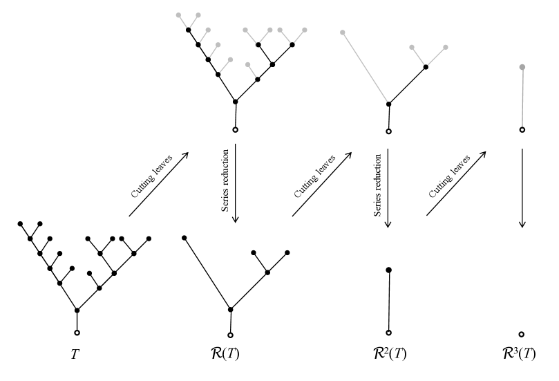
Figure 1. Example of pruning and Horton-Strahler ordering for a tree $T\in{\mathcal{L}}_{\rm plane}$. The figure shows the two stages of pruning operation – cutting the leaves (top row), and consecutive series reduction (bottom row). The initial tree $T$ is shown in the leftmost position of the bottom row. The gray color in the top row depicts vertices and edges being pruned. The order of the tree is ${\sf k}(T)=3$, since it is eliminated in three prunings, ${\mathcal{R}}^{3}(T)=\phi$.

Pruning partitions the tree space ${\mathcal{T}}$ into exhaustive and mutually exclusive set of subspaces ${\mathcal{H}}_{K}$ of trees of order $K\geq 0$ such that ${\mathcal{R}}({\mathcal{H}}_{K+1})={\mathcal{H}}_{K}$. Here ${\mathcal{H}}_{0}=\{\phi\}$, ${\mathcal{H}}_{1}$ consists of a single tree comprised of a root and a leaf connected by an edge, and all other subspaces ${\mathcal{H}}_{K}$, $K\geq 2$, consist of an infinite number of trees.

Definition 2 (Horton-Strahler terminology).

We introduce the following definitions related to the Horton-Strahler order of a tree (see Fig. 2):

1. For any non-root vertex $v$ in $T\in{\mathcal{T}}\setminus\{\phi\}$, a subtree $T_{v}$ of $T$ is defined as the only subtree in $T$ rooted at the parental vertex $p(v)$ of $v$, and comprised by $v$ and all its descendant vertices together with their parental edges (Fig. 2b).

2. The Horton-Strahler order ${\sf k}(v)$ of a vertex $v\in T$ coincides with the order of the subtree $T_{v}\in T$ (Fig. 2a).

3. The parental edge of a vertex has the same order as the vertex.

4. A connected sequence of vertices of the same order together with their parental edges is called a branch (Fig. 2a).

5. The branch vertex closest to the root is called the initial vertex of a branch (Fig. 2a).

6. For the initial vertex $v$ of a branch of order $K\leq{\sf k}(T)$, a subtree of $T_{v}$ is called a complete subtree of order $K$ (Fig. 2b). The single complete subtree of order ${\sf k}(T)$ coincides with $T$. (All subtrees of order ${\sf k}=1$ are complete.)

Remark 1.

Equivalently, the Horton-Strahler ordering can be done by hierarchical counting [5, 10, 24, 20, 19, 4]. In this approach, each leaf is assigned order ${\sf k}({\rm leaf})=1$. An internal vertex $p$ whose children have orders $i$ and $j$ is assigned the order

$${\sf k}(p)=\max\left(i,j\right)+\delta_{ij}=\lfloor\log_{2}(2^{i}+2^{j})\rfloor,$$

where $\delta_{ij}$ is the Kronecker’s delta and $\lfloor x\rfloor$ denotes the maximal integer less than or equal to $x$. The Horton-Strahler order of the tree is ${\sf k}(T)=\max\limits_{v}{\sf k}(v)$, where the maximum is taken over all non-root vertices of $T\in{\mathcal{T}}\setminus\{\phi\}$.

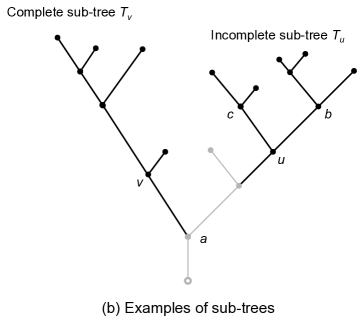
Figure 2. Illustration of the Horton-Strahler terminology (Def. 2) in a tree $T$ of order ${\sf k}(T)=3$. (a) A tree root, a branch, and an initial vertex of a branch. The numbers indicate the Horton-Strahler orders of the vertices. In particular, we have $N_{1}=10$, $N_{2}=3$, $N_{3}=1$, and $N_{1,2}=3$, $N_{1,3}=1$, $N_{2,3}=1$. (b) Examples of a complete ($T_{v}$) and incomplete ($T_{u}$) subtrees. The subtree $T_{u}$ is incomplete since $u$ is not the initial vertex of a branch. The tree shown in this panel has four complete subtrees of order ${\sf k}\geq 2$: $T_{v}$ of order 2, $T_{b}$ of order 2, $T_{c}$ of order 2, and $T_{a}=T$ of order 3.

2.2. Labeling tree vertices

Sometimes we will need to label the vertices and edges of a tree (e.g., for selecting a branch or vertex uniformly). The vertices of a planar tree can be labeled by numbers $1,\dots,\#T$ ($\#T$ denoting the total number of vertices in $T$) in order of depth-first search. We also assume that label of the parental edge for each vertex is taken from that vertex.

For a tree with no embedding, labeling is done by selecting a suitable embedding and then using the depth-first search labeling as above. Such embedding should be properly aligned with the pruning operation, as we describe in the following definition.

Definition 3 (Proper embedding).

An embedding function $\textsc{embed}:{\mathcal{T}}\to{\mathcal{T}}_{\rm plane}$ (${\mathcal{L}}\to{\mathcal{L}}_{\rm plane}$) is called proper if for any $T\in{\mathcal{T}}$ $(T\in{\mathcal{L}})$

$${\mathcal{R}}\left(\textsc{embed}(T)\right)=\textsc{embed}\left({\mathcal{R}}(T)\right),$$

where the pruning on the left-hand side is in ${\mathcal{T}}_{\rm plane}$ (${\mathcal{L}}_{\rm plane}$) and pruning on the right-hand side is in ${\mathcal{T}}$ (${\mathcal{L}})$.

A proper embedding for a tree with no edge lengths can be done using the following induction construction. A tree of order ${\sf k}=1$ assumes a unique embedding. A tree of order ${\sf k}=2$ is embedded by branching all its side-branches of order 1 to the right. Assuming there exists a proper embedding for trees of order ${\sf k}\leq K$, we construct the labeling for a tree of order $K+1$. All its side-branches (of any order) branch to the right. To embed the (only) two merging complete subtrees, $\tau_{1}\neq\tau_{2}$, of order $K$, we consider their farthest non-identical pruning descendants: trees $d_{i}={\mathcal{R}}^{k}(\tau_{i})$, $i=1,2$ obtained by the maximal possible number $k$ of pruning iterations such that $d_{1}\neq d_{2}$. The number $0\leq k\leq K-2$ is well defined since all trees of order 1, which is the unltimate pruning limit, coincide. By construction, the trees $d_{i}$ differ only by the number of side-branches of order 1 attached to the tree $d_{0}={\mathcal{R}}^{k+1}(\tau_{i})$, which already has proper embedding. Consider the numbers of order-1 side-branches within each edge of $d_{0}$, in the order of its labeling: $(n^{(i)}_{1},\dots,n^{(i)}_{\#d_{0}})$. The tree whose sequence has the smallest first non-coinciding number, will branch to the right.

A proper embedding for a tree $T\in{\mathcal{L}}$ with edge length is constructed in the same fashion, with the only correction. From the two merging complete subtrees of order $K$ with the same combinatorial structure, the one with the shortest root edge branches to the right. This definition covers the situation of atomless length distribution, which is of primary interest to us.

3. Tree Self-Similarity

This section defines self-similarity for combinatorial and metric trees. The term self-similarity is associated with invariance of a tree distribution with respect to the pruning operation ${\mathcal{R}}$ introduced in Sect. 2.1. The prune-invariance alone, however, is often insufficient to generate interesting families of trees. This necessitates an additional property – coordination of conditional measures on subspaces of trees of a given order. Coordination together with prune-invariance constitutes the self-similarity studied in this work.

We start in Sect. 3.1 with a weak form of self-similarity that only considers the average values of selected branch statistics; it was introduced in [11]. Section 3.3 discusses a stronger version of self-similarity that operates with tree distributions. Self-similarity of metric trees is presented in Sect. 3.5.

3.1. Mean self-similarity of a combinatorial tree

Let ${\mathcal{H}}_{K}\subset{\mathcal{T}}$ be the subspace of trees of Horton-Strahler order $K\geq 0$. Naturally, ${\mathcal{H}}_{K}\bigcap{\mathcal{H}}_{K^{\prime}}=\emptyset$ if $K\neq K^{\prime}$, and $\bigcup\limits_{K\geq 1}{\mathcal{H}}_{K}={\mathcal{T}}$. Consider a set of conditional probability measures $\{\mu_{K}\}_{K\geq 0}$ each of which is defined on ${\mathcal{H}}_{K}$ by $\mu_{K}(T)=\mu(T|T\in{\mathcal{H}}_{K})$ and let $p_{K}=\mu({\mathcal{H}}_{K})$. Then $\mu$ is represented as a mixture of the conditional measures:

(2) $$\mu=\sum_{K=1}^{\infty}p_{K}\mu_{K}.$$

We write ${\sf E}_{K}(\cdot)$ for the mathematical expectation with respect to $\mu_{K}$. Let $N_{k}=N_{k}[T]$ denotes the number of branches of order $k$ in a tree $T\in{\mathcal{T}}$ (see Fig. 2a). We define the average Horton numbers for subspace ${\mathcal{H}}_{K}$ as

$${\mathcal{N}}_{k}[K]={\sf E}_{K}(N_{k}),\quad 1\leq k\leq K,\quad K\geq 1.$$

Let $N_{i,j}=N_{i,j}[T]$ denote the number of instances when an order-$i$ branch merges with an order-$j$ branch, $1\leq i<j$, in a tree $T$ (see Fig. 2a). Such branches are referred to as side-branches of order $\{i,j\}$. Consider the respective expectation ${\mathcal{N}}_{i,j}[K]:={\sf E}_{K}(N_{i,j})$. The Tokunaga coefficients $T_{i,j}[K]$ for subspace ${\mathcal{H}}_{K}$ are defined as

(3) $$T_{i,j}[K]=\frac{{\mathcal{N}}_{i,j}[K]}{{\mathcal{N}}_{j}[K]},\quad 1\leq i<j\leq K.$$

The Tokunaga coefficient $T_{i,j}[K]$ is hence reflects the average number of side-branches of order $\{i,j\}$ per branch of order $j$ in a tree of order $K$.

Next, we introduce a property that ensures independence of the side-branch structure of a tree order.

Definition 4 (Mean coordination).

A set of measures $\{\mu_{K}\}_{K\geq 1}$ on $\{{\mathcal{H}}_{K}\}_{K\geq 1}$ is called mean coordinated if $T_{i,j}:=T_{i,j}[K]$ for all $K\geq 2$ and $1\leq i<j\leq K$. A measure $\mu$ on ${\mathcal{T}}$ is called mean coordinated if the respective conditional measures $\{\mu_{K}\}$, as in Eq. (2), are mean coordinated.

For a mean coordinated measure $\mu$, the Tokunaga matrix $\mathbb{T}_{K}$ is a $K\times K$ matrix

$$\mathbb{T}_{K}=\left[\begin{array}[]{ccccc}0&T_{1,2}&T_{1,3}&\ldots&T_{1,K}\\ 0&0&T_{2,3}&\ldots&T_{2,K}\\ 0&0&\ddots&\ddots&\vdots\\ \vdots&\vdots&\ddots&0&T_{K-1,K}\\ 0&0&\dots&0&0\end{array}\right],$$

which coincides with the restriction of any larger-order Tokunaga matrix $\mathbb{T}_{M}$, $M>K$, to the first $K\times K$ entries.

Definition 5 (Toeplitz property).

A set of measures $\{\mu_{K}\}_{K\geq 1}$ on $\{{\mathcal{H}}_{K}\}_{K\geq 1}$ is said to satisfy the Toeplitz property if $T_{i,j}[K]=T_{j-i}[K]$ for each $K\geq 2$ and some sequence $T_{k}[K]\geq 0$, $k=1,2,\dots$. The elements of the sequences $T_{k}[K]$ are also referred to as Tokunaga coefficients, which does not create confusion with $T_{i,j}[K]$. A measure $\mu$ on ${\mathcal{T}}$ is said to satisfy the Toeplitz property if the respective conditional measures $\{\mu_{K}\}$, as in Eq. (2), satisfy the Toeplitz property.

Definition 6 (Mean self-similarity).

A measure $\mu$ on ${\mathcal{T}}$ is called mean self-similar if it is mean coordinated and satisfies the Toeplitz property.

For a mean self-similar measure the Tokunaga matrix $\mathbb{T}_{K}$ becomes Toeplitz:

$$\mathbb{T}_{K}=\left[\begin{array}[]{ccccc}0&T_{1}&T_{2}&\ldots&T_{K-1}\\ 0&0&T_{1}&\ldots&T_{K-2}\\ 0&0&\ddots&\ddots&\vdots\\ \vdots&\vdots&\ddots&0&T_{1}\\ 0&0&\dots&0&0\end{array}\right].$$

Pruning ${\mathcal{R}}$ decreases the Horton-Strahler order of each vertex (and hence of each branch) by unity; in particular

(4) $$N_{k}[T]=N_{k-1}\left[{\mathcal{R}}(T)\right],\quad k\geq 2,$$

(5) $$N_{i,j}[T]=N_{i-1,j-1}\left[{\mathcal{R}}(T)\right],\quad 2\leq i<j.$$

Consider measure $\mu^{{\mathcal{R}}}_{K}$ induced on ${\mathcal{H}}_{K}$ by the pruning operator:

$$\mu^{{\mathcal{R}}}_{K}(A)=\mu_{K+1}\left({\mathcal{R}}^{-1}(A)\right)\quad\forall A\subset{\mathcal{H}}_{K}.$$

The Tokunaga coefficients computed on ${\mathcal{H}}_{K}$ using the induced measure $\mu^{{\mathcal{R}}}_{K}$ are denoted by $T_{i,j}^{{\mathcal{R}}}[K]$. Formally,

(6) $$T_{i,j}^{{\mathcal{R}}}[K]=T_{i+1,j+1}[K+1]=\frac{{\mathcal{N}}_{i+1,j+1}[K+1]}{{\mathcal{N}}_{j+1}[K+1]}.$$

Definition 7 (Mean prune-invariance).

A set of measures $\{\mu_{K}\}_{K\geq 1}$ on $\{{\mathcal{H}}_{K}\}_{K\geq 1}$ is called mean prune-invariant if $T_{i,j}[K]=T_{i,j}^{{\mathcal{R}}}[K]$ (equivalently, $T_{i,j}[K]=T_{i+1,j+1}[K+1]$), for any $K\geq 2$ and all $1\leq i<j\leq K$. A measure $\mu$ on ${\mathcal{T}}$ is called mean prune-invariant if the respective conditional measures $\{\mu_{K}\}$, as in Eq. (2), are mean prune-invariant.

Definition 8 (Mean self-similarity).

A probability measures $\mu$ on ${\mathcal{T}}$ is called mean self-similar with respect to pruning ${\mathcal{R}}$ if it is coordinated and mean prune-invariant.

Proposition 1.

Definitions 6 and 8 of mean self-similarity are equivalent.

This equivalence was proven in [11]. Its validity is readily seen from the diagram of Fig. 3a, which shows relations among the quantities $T_{i,j}[K]$, $T_{i,j}[K+1]$, and $T_{i+1,j+1}[K+1]$ involved in the definitions of coordination, prune-invariance, and Toeplitz property. Moreover, we observe that if any two of these properties hold, the third also holds. The Venn diagram of Fig. 3b illustrates the relation among mean coordination, mean prune-invariance, Toeplitz property and mean self-similarity in the space ${\mathcal{T}}$. In this work, we refer to the mean self-similarity with respect to pruning ${\mathcal{R}}$ simply as mean self-similarity.

Figure 3. Relations among mean coordination, mean prune-invariance, and Toeplitz property. (a) Pairwise equalities among the quantities $T_{i,j}[K]$, $T_{i,j}[K+1]$, and $T_{i+1,j+1}[K+1]$ involved in the definitions of mean coordination, mean prune-invariance, and Toeplitz property. (b) Venn diagram of the space ${\mathcal{T}}$ illustrating the relation among mean coordination (left triangle), mean prune-invariance (right triangle), and Toeplitz property (bottom triangle). The mean self-similarity (inner dark triangle) is formed by the intersection of any pair of the three properties.

A variety of mean self-similar measures can be constructed for an arbitrary sequence of Tokunaga coefficients $T_{k}\geq 0$, $k\geq 1$. Next, we give a natural example [11].

3.2. Example of a mean self-similar measure: Independent random attachment

The subspace ${\mathcal{H}}_{1}$, which consists of a single-leaf tree, possesses a trivial unity mass measure. To construct a random tree from ${\mathcal{H}}_{2}$, we select a discrete probability distribution $P_{1,2}(n)$, $n=0,1,\dots$, with the mean value $T_{1}$. A random tree $T\in{\mathcal{H}}_{2}$ is obtained from the single-leaf tree $\tau_{1}$ of order 1 via the following two operations. First, we attach two offspring vertices to the leaf of $\tau_{1}$. This creates a tree of order 2 with no side-branches – one internal vertex of degree 3, two leaves, and the root. Second, we draw the number $\tilde{N}_{1,2}$ from the distribution $P_{1,2}$, and attach $\tilde{N}_{1,2}$ vertices to this tree so that they form side-branches of order $\{1,2\}$.

In general, to construct a random tree $T\in{\mathcal{H}}_{K}$ of order $K\geq 2$ we select a set of discrete probability distributions $P_{k,K}(n)$, $k=1,...,K-1$, on $\mathbb{Z}_{+}$ with the respective mean values $T_{k}$. A random tree $T\in{\mathcal{H}}_{K}$ is constructed by adding branches of order 1 (leaves) to a random tree $\tau\in{\mathcal{H}}_{K-1}$. First, we add two new child vertices to every leaf of $\tau$ hence producing a tree $\tilde{T}$ of order $K$ with no side-branches of order 1. Second, for each branch $b$ of order $2\leq j\leq K$ in $\tilde{T}$ we draw a random number $\tilde{N}_{1,j}(b)$ from the distribution $P_{j-1,K}$ and attach $\tilde{N}_{1,j}(b)$ new child vertices to this branch so that they form side-branches of order $\{1,j\}$. Each new vertex is attached in a random order with respect to the existing side-branches. Specifically, we notice that $m\geq 0$ side-branches attached to a branch of order $j$ are uniquely associated with $m+1$ edges within this branch. The attachment of the new $\tilde{N}_{1,j}(b)$ vertices among the $m+1$ edges is given by the equiprobable multinomial distribution with $m+1$ categories and $\tilde{N}_{1,j}(b)$ trials.

The procedure described above generates a set of measures $\{\mu_{K}\}_{K\geq 1}$ on $\{{\mathcal{H}}_{K}\}_{K\geq 1}$ that are mean coordinated by construction (recall that the mean values $T_{k}$ of the distributions $P_{k,K}$ are independent of $K$).

Furthermore, observe that

$$N_{i,j}=\sum_{b_{i}=1}^{N_{j}}\tilde{N}_{1,j-i+1}(b_{i}),$$

$${\mathcal{N}}_{i,j}[K] = {\sf E}_{K}(N_{i,j})={\sf E}_{K}\left({\sf E}_{K}(N_{i,j}|N_{j})\right)={\sf E}_{K}(N_{j}\,T_{j-i})$$

$$= T_{j-i}\,{\sf E}_{K}(N_{j})=T_{j-i}\,{\mathcal{N}}_{j}[K],$$

and hence $T_{i,j}[K]={\mathcal{N}}_{i,j}[K]/{\mathcal{N}}_{j}[K]=T_{j-i}$, so the tree is mean self-similar, according to Def. 6.

Remark 2.

The properties introduced in this section – mean coordination, mean prune-invariance, Toeplitz, and mean self-similarity – are completely specified by a set of conditional measures $\{\mu_{K}\}$, and are independent of the randomization probabilities $p_{K}=\mu({\mathcal{H}}_{K})$, see Eq. (2).

Remark 3.

The idea of relating tree mean self-similarity (Def. 8) to mean prune-invariance (Def. 7) is quite intuitive (see also [4]). Much less so is the requirement of mean coordination of conditional measures (Def. 4), included in the definition of mean self-similarity. This requirement is motivated by our goal to bridge the measure-theoretic definition of self-similarity via the pruning operation (Def. 8) to a statistical definition via the branch counting (Def. 6). In applications, when a handful of trees of different orders is observed, the coordination assumption allows one to estimate the Tokunaga coefficients $T_{i,j}$ and make inference regarding the Toeplitz property; see [20, 19, 6, 29]. The absence of coordination, at the same time, opens a possibility of having a variety of prune-invariant measures with no Toeplitz constraint, which are hardly treatable in applications. To construct a simplest such measure, let select any tree $T_{2}$ from the pre-image of the only tree $T_{1}\in{\mathcal{H}}_{1}$ of order $K=1$ under the pruning operation: $T_{2}\in{\mathcal{R}}^{-1}(T_{1})\in{\mathcal{H}}_{2}$. In a similar fashion, select any tree $T_{K+1}$ from the pre-image of $T_{K}$ for $K\geq 2$. This gives us a collection of trees $T_{K}\in{\mathcal{H}}_{K}$, $K\geq 1$ such that ${\mathcal{R}}(T_{K+1})=T_{K}$. Assign the full measure on ${\mathcal{H}}_{K}$ to $T_{K}$: $\mu_{K}(T_{K})=1$. By construction, the measures $\{\mu_{K}\}$ are mean prune-invariant. They, however, may satisfy neither the mean coordination nor the Toeplitz property. This construction illustrates how one can produce rather obscure collections of trees that are mean prune-invariant, providing a motivation for the coordination requirement adopted in this work.

3.3. Self-similarity of a combinatorial tree

This section introduces a distribution-based approach to self-similarity.

Definition 9 (Prune-invariance).

Consider a probability measure $\mu$ on ${\mathcal{T}}$ such that $\mu(\phi)=0$. Let $\nu(T)=\mu\circ{\mathcal{R}}^{-1}(T)=\mu\big{(}{\mathcal{R}}^{-1}(T)\big{)}$. (Note that $\nu(\phi)>0$.) Measure $\mu$ is called invariant with respect to the pruning operation (prune-invariant) if for any tree $T\in{\mathcal{T}}$ we have

(8) $$\nu\left(T~{}|T\neq\phi\right)=\mu(T).$$

Proposition 2.

Let $\mu$ be a prune-invariant measure on ${\mathcal{T}}$. Then the distribution of orders, $p_{K}=\mu({\mathcal{H}}_{K})$, is geometric:

(9) $$p_{K}=p\left(1-p\right)^{K-1},\quad K\geq 1,$$

where $p=p_{1}=\mu({\mathcal{H}}_{1})$, and for any $T\in{\mathcal{H}}_{K}$

(10) $$\mu_{K+1}\left({\mathcal{R}}^{-1}(T)\right)=\mu_{K}(T).$$

Proof.

Pruning ${\mathcal{R}}$ is a shift operator on the sequence of subspaces $\{{\mathcal{H}}_{k}\}$:

(11) $${\mathcal{R}}^{-1}({\mathcal{H}}_{K-1})={\mathcal{H}}_{K},~{}K\geq 2.$$

The only tree eliminated by pruning is the tree of order 1: $\{\tau:{\mathcal{R}}(\tau)=\phi\}={\mathcal{H}}_{1}.$ This allows to rewrite (8) for any $T\neq\phi$ as

(12) $$\mu\left({\mathcal{R}}^{-1}(T)\right)=\mu(T)\left(1-\mu({\mathcal{H}}_{1})\right).$$

Combining (11) and (12) we find for any $K\geq 2$

(13) $$\mu\left({\mathcal{H}}_{K}\right)\stackrel{{\scriptstyle{\rm by}~{}\eqref{H_shift}}}{{=}}\mu\left({\mathcal{R}}^{-1}({\mathcal{H}}_{K-1})\right)\stackrel{{\scriptstyle{\rm by}~{}\eqref{def:pi1}}}{{=}}\left(1-\mu({\mathcal{H}}_{1})\right)\mu({\mathcal{H}}_{K-1}),$$

which establishes (9). Next, for any tree $T\in{\mathcal{H}}_{K}$ we have

$$\mu(T)=\mu({\mathcal{H}}_{1})\left(1-\mu({\mathcal{H}}_{1})\right)^{K-1}\mu_{K}(T),$$

$$\mu\left({\mathcal{R}}^{-1}(T)\right)=\mu({\mathcal{H}}_{1})\left(1-\mu({\mathcal{H}}_{1})\right)^{K}\mu_{K+1}\left({\mathcal{R}}^{-1}(T)\right).$$

Together with (12) this implies (10). ∎

Proposition 2 shows that a prune-invariant measure $\mu$ is completely specified by its conditional measures $\mu_{K}$ and the mass $p=\mu({\mathcal{H}}_{1})$ of the tree of order $K=1$. The same result was obtained for Galton-Watson trees in [4, Thm. 3.5].

Next, we introduce a distributional analog of the mean coordination property; see Def. 4 and Remark 3. Specifically, we assume that a complete subtree $T_{K}$ of a given order $K$ randomly selected from a random tree $T_{H}$ of order $H\geq K$ has a common distribution independent of $H$. Since a tree $T_{K}$ of order $K$ has only one complete subtree of order $K$, which coincides with $T_{K}$, this common distribution must be $\mu_{K}$. Formally, consider the following process of selecting a uniform random complete subtree ${\sf subtree}_{K,H}$ of order $K$ from a random tree $T_{H}\in{\mathcal{H}}_{H}$. First, select a random tree $T_{H}$ according to the conditional measure $\mu_{H}$. Label all complete subtrees of order $K$ in $T_{H}$ in order of proper labeling of Sect. 2.2, and select a uniform random subtree, which we denote ${\sf subtree}_{K,H}$. By construction, ${\sf subtree}_{K,H}\in{\mathcal{H}}_{K}$; we denote the corresponding sampling measure on ${\mathcal{H}}_{K}$ by $\mu^{H}_{K}$.

Definition 10 (Coordination).

A set of measures $\{\mu_{K}\}_{K\geq 1}$ on $\{{\mathcal{H}}_{K}\}_{K\geq 1}$ is called coordinated if $\mu^{H}_{K}(T)=\mu_{K}(T)$ for any $K\geq 1$, $H\geq K$, and $T\in{\mathcal{H}}_{K}$. A measure $\mu$ on ${\mathcal{T}}$ is called coordinated if the respective conditional measures $\{\mu_{K}\}$, as in Eq. (2), are coordinated.

Example 1.

The space of finite binary Galton-Watson trees has the coordination property. Recall that a random binary Galton-Watson tree starts with a single progenitor (root) and increases its depth in discrete steps: at every step each existing vertex can either split in two with probability $p_{2}$ or become a leaf (disappear) with probability $p_{0}=1-p_{2}$. We denote the resulting tree distribution on ${\mathcal{T}}$ by $\mathcal{GW}(p_{0},p_{2})$. This Markovian generation mechanism creates complete subtrees of the same structure, independently of the tree order. This implies coordination.

Definition 11 (Combinatorial self-similarity).

A probability measure $\mu$ on ${\mathcal{T}}$ is called (combinatorially) self-similar with respect to pruning ${\mathcal{R}}$ if it is coordinated and prune-invariant.

In this work, we refer to combinatorial self-similarity with respect to pruning ${\mathcal{R}}$ simply as combinatorial self-similarity. It was established in [4] that critical binary Galton-Watson trees $\mathcal{GW}(1/2,1/2)$ are prune-invariant. Together with coordination (see Example 1), this implies combinatorial self-similarity. It also has been shown in [4] that non-critical binary Galton-Watson trees ($p_{0}\neq 1/2$) are not prune-invariant. This gives an example of coordinated measures that are not prune-invariant. Prune-invariant measures with no coordination can be easily constructed following the approach of Remark 3. To make that construction consistent with the definition of distributional prune-invariance (Def. 9), each tree $T_{K}\in{\mathcal{H}}_{K}$ must be assigned the probability $p_{K}=p(1-p)^{K-1}$.

3.4. Horton law in self-similar trees

We say that a random tree $T$ satisfies a strong Horton law if the respective sequence ${\mathcal{N}}_{k}[K]$ of branch numbers decays in geometric fashion as $k$ increases. Formally, we require

(14) $$\lim_{K\to\infty}\frac{{\mathcal{N}}_{k}[K]}{{\mathcal{N}}_{1}[K]}=R^{1-k},\text{ for any }k\geq 1.$$

Horton law and its ramifications, which epitomize scale-invariance of dendritic hierarchical structures, are indispensable in hydrology (e.g., [23, 20, 6]) and have been reported in biology and other areas; see [19, 13] and references therein. It has been shown in [12] that the tree that describes a trajectory Kingman’s coalescent process with $N$ particles obeys a weaker version of Horton law as $N\to\infty$, and that the first pruning of this tree for any finite $N$ is equivalent to a level set tree of a white noise (see Sect. 4 for definitions).

A necessary and sufficient condition for the strong Horton law in a mean self-similar tree has been established in [11]:

$$\limsup_{k\to\infty}T_{k}^{1/k}<\infty.$$

The Horton exponent $R$ in this case is given by $R=1/w_{0}$, where $w_{0}$ is the only real root of

$$\hat{t}(z)=-1+2z+\sum_{k=1}^{\infty}z^{k}\,T_{k}$$

within the interval $(0,1/2]$. Informally, this means that any mean self-similar tree with a “tamed” sequence of Tokunaga coefficients satisfies the strong Horton law.

3.5. Self-similarity of a tree with edge lengths

Consider a tree $T\in{\mathcal{L}}$ with edge lengths given by a positive vector $l_{T}=(l_{1},\dots,l_{\#T})$ and let $\textsc{length}(T)=\sum_{i}l_{i}$. We assume that the edges are labeled in a proper way as described in Sect. 2.2. A tree is completely specified by its combinatorial shape $\textsc{shape}(T)$ and edge length vector $l_{T}$. The edge length vector $l_{T}$ can be specified by distribution $\chi(\cdot)$ of a point $x_{T}=(x_{1},\dots,x_{\#T})$ on the simplex $\sum_{i}x_{i}=1$, $0<x_{i}\leq 1$, and conditional distribution $F(\cdot|x_{T})$ of the tree length $\textsc{length}(T)$, where

$$l_{T}=x_{T}\times\textsc{length}(T).$$

A measure $\eta$ on ${\mathcal{L}}$ is a joint distribution of tree’s combinatorial shape and its edge lengths; it has the following component measures.

$${\rm Combinatorial~{}shape:}\quad\mu(\tau)={\sf Law}\left(\textsc{shape}(T)=\tau\right),$$

$${\rm Relative~{}edge~{}lengths:}\quad\chi_{\tau}(\bar{x})={\sf Law}\left(x_{T}=\bar{x}\,|\,\textsc{shape}(T)=\tau\right),$$

$${\rm Total~{}tree~{}length:}\quad F_{\tau,\bar{x}}(\ell)={\sf Law}\left(\textsc{length}(T)=\ell\,|\,x_{T}=\bar{x},~{}\textsc{shape}(T)=\tau\right).$$

The definition of self-similarity for a tree with edge lengths builds on its analog for combinatorial trees in Sect. 3.3. The combinatorial notions of coordination (Def. 10) and prune-invariance (Def. 9), which we refer to as coordination and prune-invariance in shapes, are complemented with analogous properties in edge lengths. Formally, we denote by $\mu^{H}_{K}(\tau)$, $\chi^{H}_{\tau}(\bar{x})$, and $F^{H}_{\tau,\bar{x}}(\ell)$ the component measures for a uniform complete subtree ${\sf subtree}_{K,H}$. (Notice that the subtree order $K$ is completely specified by the tree shape $\tau$, which explains the absence of subscript $K$ in the component measures for subtree length). We also consider the distribution of edge lengths after pruning:

$$\Xi_{\tau}(\bar{x})={\sf Law}\left(x_{{\mathcal{R}}(T)}=\bar{x}\,|\,\textsc{shape}\big{(}{\mathcal{R}}(T)\big{)}=\tau\right)$$

and

$$\Phi_{\tau,\bar{x}}(\ell)={\sf Law}\left(\textsc{length}\big{(}{\mathcal{R}}(T)\big{)}=\ell\,|\,x_{{\mathcal{R}}(T)}=\bar{x},~{}\textsc{shape}\big{(}{\mathcal{R}}(T)\big{)}=\tau\right).$$

Finally, we adopt here the notation ${\mathcal{H}}_{K}$ for a subspace of trees of order $K\geq 1$ from ${\mathcal{L}}$, and consider conditional measures $\mu_{K}(\tau)=\mu(\tau|{\sf k}(\tau)=K)$, $K\geq 1$, for a tree $\tau\in{\mathcal{L}}$.

Definition 12 (Self-similarity of a tree with edge lengths).

We call a measure $\eta$ on ${\mathcal{L}}$ self-similar with respect to pruning ${\mathcal{R}}$ if the following conditions hold

• The measure is coordinated in shapes. This means that for every $K\geq 1$ and every $H\geq K$ we have

  $$\mu^{H}_{K}(\tau)=\mu_{K}(\tau)\qquad\forall\tau\in{\mathcal{H}}_{K}.$$

• The measure is coordinated in lengths. This means that for every $K\geq 1$, $H\geq K$, and $\tau\in{\mathcal{H}}_{K}$ we have

  $$\chi^{H}_{\tau}(\bar{x})=\chi_{\tau}(\bar{x})\quad\bar{x}\text{-}a.s.~{},$$

  and for every given $\bar{x}$,

  $$F^{H}_{\tau,\bar{x}}(\ell)=F_{\tau,\bar{x}}(\ell)\quad\ell\text{-}a.s.$$

• The measure is prune-invariant in shapes. This means that for $\nu=\mu\circ{\mathcal{R}}^{-1}$ we have

  $$\mu(\tau)=\nu(\tau|\tau\neq\phi).$$

• The measure is prune-invariant in lengths. This means that

  $$\Xi_{\tau}(\bar{x})=\chi_{\tau}(\bar{x})$$

  and there exists a scaling exponent $\zeta>0$ such that for any combinatorial tree $\tau\in{\mathcal{T}}$ we have

  $$\Phi_{\tau,\bar{x}}(\ell)=\zeta^{-1}F_{\tau,\bar{x}}\left(\frac{\ell}{\zeta}\right).$$

In this work, we refer to self-similarity with respect to pruning ${\mathcal{R}}$ simply as self-similarity. Section 5 below introduces a rich class of measures that satisfy this definition.

4. Tree Representation of Continuous Functions

We review here the results of [15, 18, 21, 28] on tree representation of continuous functions. This allows us to apply the self-similarity concepts to time series and motivates discussion in Sects. 5.6, 5.7 below.

4.1. Harris path

For any embedded tree $T\in{\mathcal{L}}_{\rm plane}$ with edge lengths, the Harris path is defined as a piece-wise linear function [9, 21]

$$H_{T}(t)\,:\,[0,2\cdot\textsc{length}(T)]\to\mathbb{R}$$

that equals the distance from the root traveled along the tree $T$ in the depth-first search, as illustrated in Fig. 4. For a tree $T$ with $n$ leaves, the Harris path $H_{T}(t)$ is a piece-wise linear positive excursion that consists of $2n$ linear segments with alternating slopes $\pm 1$ [21].

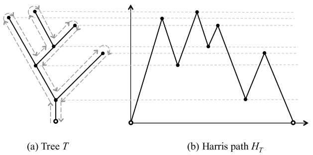
Figure 4. (a) Tree $T$ and its depth-first search illustrated by dashed arrows. (b) Harris path $H_{T}(t)$ for the tree $T$ of panel (a).

4.2. Level set tree

Consider a continuous function $X_{t}$, $t\in[a,b]$ with a finite number of distinct local minima. The level set $\mathcal{L}_{\alpha}\left(X_{t}\right)$ is defined as the pre-image of the function values above $\alpha$:

$$\mathcal{L}_{\alpha}\left(X_{t}\right)=\{t\,:\,X_{t}\geq\alpha\}.$$

The level set $\mathcal{L}_{\alpha}$ for each $\alpha$ is a union of non-overlapping intervals; we write $|\mathcal{L}_{\alpha}|$ for their number. Notice that $|\mathcal{L}_{\alpha}|=|\mathcal{L}_{\beta}|$ as soon as the interval $[\alpha,\,\beta]$ does not contain a value of local extrema of $X_{t}$ and $0\leq|\mathcal{L}_{\alpha}|\leq n$, where $n$ is the number of the local maxima of $X_{t}$.

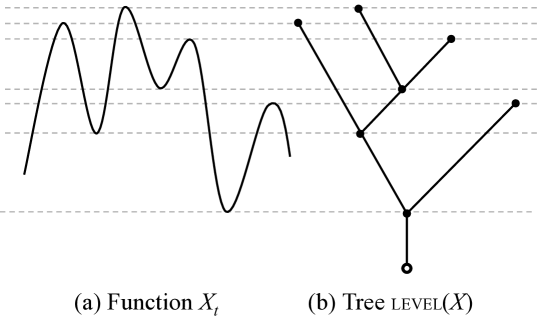
Figure 5. Function $X_{t}$ (panel a) with a finite number of local extrema and its level-set tree $\textsc{level}(X)$ (panel b).

The level set tree $\textsc{level}(X_{t})\in{\mathcal{L}}_{\rm plane}$ is a tree that describes the topology of the level sets $\mathcal{L}_{\alpha}$ as a function of threshold $\alpha$, as illustrated in Fig. 5. Specifically, there are bijections between (i) the leaves of $\textsc{level}(X_{t})$ and the local maxima of $X_{t}$, (ii) the internal (parental) vertices of $\textsc{level}(X_{t})$ and the local minima of $X_{t}$ (excluding possible local minima at the boundary points), and (iii) the pair of subtrees of $\textsc{level}(X_{t})$ rooted at the parental vertex that corresponds to a local minima $X_{t^{*}}$ and the first positive excursions (or meanders bounded by $t=a$ or $t=b$) of $X_{t}-X_{t^{*}}$ to right and left of $t^{*}$. Every edge in the tree is assigned a length equal the difference of the values of $X_{t}$ at the local extrema that correspond to the vertices adjacent to this edge according to the bijections (i) and (ii) above. The lowest internal local minimum (achieved for $a<t<b$) corresponds to the first descendant of the root, see Fig. 5. If the global minimum is achieved on the interval boundary ($t=a$ or $t=b$), then it corresponds to the tree root; otherwise, we artificially add a root to the tree, with an arbitrary root edge length; this situation is illustrated in Fig. 5.

By construction, the level-set tree $\textsc{level}(X_{t})$ is completely determined by the sequence of the values of local extrema of $X_{t}$, and is independent of timing of those extrema, as soon as their order is preserved. This means, for instance, that if $g(t)$ is a continuous and monotone increasing function on $[a,b]$, then the following trees are equivalent:

$$\textsc{level}(X_{t})=\textsc{level}\left(X_{g(t)}\right).$$

Hence, without loss of generality we can focus on the level set trees of continuous functions with alternating slopes $\pm 1$. By ${\mathcal{E}}^{\rm ex}$ we denote the space of all positive piece-wise linear continuous finite excursions with alternating slopes $\pm 1$.

By construction, the level set tree of an excursion from ${\mathcal{E}}^{\rm ex}$ and Harris path are reciprocal to each other as described in the following statement.

Proposition 3 (Reciprocity of Harris path and level set tree).

The Harris path $H:{\mathcal{L}}_{\rm plane}\to{\mathcal{E}}^{\rm ex}$ and the level set tree ${\textsc{level}}:{\mathcal{E}}^{\rm ex}\to{\mathcal{L}}_{\rm plane}$ are reciprocal to each other. This means that for any $T\in{\mathcal{L}}_{\rm plane}$ we have $\textsc{level}(H_{T}(t))\equiv T,$ and for any $Y_{t}\in{\mathcal{E}}^{\rm ex}$ we have $H_{\textsc{level}(Y_{t})}(t)\equiv Y_{t}.$

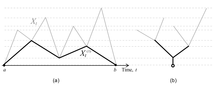
Figure 6. Pruning of a positive excursion: transition to the local minima of an excursion $X_{t}$ corresponds to pruning of the corresponding level set tree. (a) An original excursion $X_{t}$ (gray line) and linearly interpolated sequence $X^{(1)}_{t}$ of the respective local minima (black line). (b) The level set tree $\textsc{level}(X^{(1)}_{t})$ of the local minima sequence (black lines) is obtained by pruning of the level set tree $\textsc{level}(X_{t})$ of the original excursion (whole tree). The pruned edges are shown in gray – each of them corresponds to a local maximum of the original excursion.

4.3. Pruning for positive excursions

This section examines level set tree and the respective pruning for a positive continuous excursion $X_{t}$ on $[a,b]$. Formally, consider a continuous function $X_{t}$ with a finite number of local minima and such that $X_{a}=X_{b}=0$ and $X_{t}>0$ for $a<t<b$. Furthermore, consider excursion $X^{(1)}_{t}$, $t\in[a,b]$, obtained by a linear interpolation of the boundary values and the local minima of $X_{t}$; as well as functions $X^{(m)}_{t}$, $t\in[a,b]$, for $m\geq 1$, obtained by taking the local minima of $X_{t}$ iteratively $m$ times, and linearly interpolating their values together with $X_{a}=X_{b}=0$ (see Fig. 6a).

In the space of level set trees of continuous functions, the pruning ${\mathcal{R}}$ corresponds to coarsening the respective function by removing (smoothing) its local maxima, as illustrated in Fig. 6. An iterative pruning corresponds to iterative transition to the local minima.

Proposition 4 (Pruning for positive excursions, [28]).

Using the definitions of this section, the transition from a positive excursion $X_{t}$ to the respective excursion $X^{(1)}_{t}$ of its local minima corresponds to pruning of the level-set tree $\textsc{level}(X_{t})$. This is illustrated in a diagram of Fig. 7. Formally,

$$\textsc{level}\left(X^{(m)}_{t}\right)={\mathcal{R}}^{m}\left(\textsc{level}(X_{t})\right),\forall m\geq 1.$$

It is straightforward to formulate an analog of Prop. 4 without the excursion assumption (for continuous functions with a finite number of local minima). This, however, involves technicalities that are tangential to the essence of this work and will be discussed elsewhere.

Figure 7. Transition to the local minima of a function $X_{t}$ corresponds to pruning ${\mathcal{R}}$ of the corresponding level set tree $\textsc{level}(X_{t})$.

4.4. Self-similarity for time series

Consider a time series $X_{k}$, $k\in\mathbb{Z}$, with an atomless distribution of values at each $k$. Let $X_{t}$, $t\in\mathbb{R}$, be a continuous function of linearly interpolated values of $X_{k}$. We define a positive excursion of $X_{k}$ as a fragment of the time series on an interval $[l,r]$, $l,r\in\mathbb{Z}$ such that $X_{l}\geq X_{r}$ and $X_{k}>X_{l}$ for all $l<k<r$. To each positive excursion of $X_{k}$ on $[l,r]$ corresponds a positive excursion of $X_{t}$ on $[l,\tilde{r}]$, where $\tilde{r}\in(r-1,r]$ is such that $X_{\tilde{r}}=X_{l}$. This construction is illustrated in Fig. 8. The level set tree of a positive excursion of $X_{k}$ is that of the corresponding positive excursion of $X_{t}$.

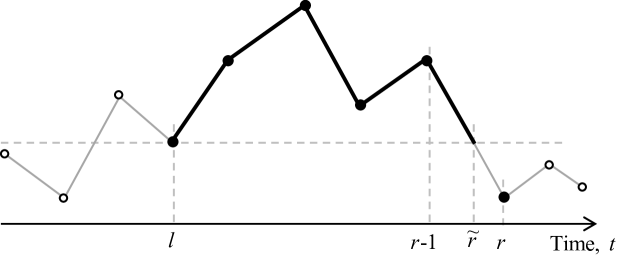
Figure 8. Excursion of a time series: illustration. The values of time series $X_{k}$ are shown by circles; the circles that form the excursion on $[l,r]$ are filled. The linear interpolation function $X_{t}$ is shown by solid line; the excursion of $X_{t}$ on $[l,\tilde{r}]$ is shown in bold.

Proposition 4 and a comment after it suggest that the problem of finding self-similar trees with edge lengths is equivalent to finding extreme-invariant processes

(15) $$X_{k}\stackrel{{\scriptstyle d}}{{=}}\zeta\,X^{(1)}_{k}\quad{\rm for~{}some~{}}\zeta>0,$$

where $X_{k}$, $k\in\mathbb{Z}$, is a time series with an atomless value distribution at every $k$ and $X^{(1)}_{k}$ is the corresponding time series of local minima. If $X_{k}$ satisfies (15), the level set tree of an excursion from $X_{k}$, considered as an element of ${\mathcal{L}}$, is self-similar according to Def. 12. The next section describes a solution to (15) that corresponds to $\zeta=2$.

4.5. Self-similarity for random walks on $\mathbb{R}$

Consider a random walk $\{X_{k}\}_{k\in\mathbb{Z}}$ with a homogeneous transition kernel $p(x,y)\equiv p(x-y)$, for any $x,y\in\mathbb{R}$, where $p(x)$ is an atomless density function. A homogeneous random walk is called symmetric if $p(x)=p(-x)$ for all $x\in\mathbb{R}$.

Lemma 1 (Pruning for random walks, [28]).

The following statements hold.

a:

The local minima of a homogeneous random walk $\{X_{k}\}_{k\in\mathbb{Z}}$ form a homogeneous random walk (with a different transition kernel in general).

b:

The local minima of a symmetric homogeneous random walk $\{X_{k}\}_{k\in\mathbb{Z}}$ form a symmetric homogeneous random walk (with a different transition kernel in general).

The transition kernel of a symmetric random walk can be represented as the even part of a probability density function $f(x)$ with support in $\mathbb{R}_{+}$:

$$p(x)=\frac{f(x)+f(-x)}{2}.$$

The following result describes the solution of the problem (15) in terms of the characteristic function of $f(x)$.

Proposition 5 (Self-similarity for a symmetric homogeneous random walk, [28]).

The local minima of a symmetric homogeneous random walk $\{X_{k}\}_{k\in\mathbb{Z}}$ with a transition kernel $~{}p(x)=\frac{f(x)+f(-x)}{2}~{}$ form a symmetric homogeneous random walk with a transition kernel

$$p^{(1)}(x)=\zeta^{-1}\,p(x/\zeta),\quad c>0$$

if and only if $\zeta=2$ and

(16) $$\Re\left[\widehat{f}(2s)\right]=\left|\frac{\widehat{f}(s)}{2-\widehat{f}(s)}\right|^{2},$$

where $\widehat{f}(s)$ is the characteristic function of $f(x)$ and $\Re[z]$ stays for the real part of $z\in\mathbb{C}$.

A solution to (16) is given for example by an exponential density $f(x)=\phi_{\lambda}(x)$ of (18) for any $\lambda>0$; a detailed discussion of exponential kernels is given in Sect. 4.6. A weaker, mean self-similarity of Defs. 6, 8 is satisfied in any symmetric random walk, as discussed in the following statement.

Theorem 1 (Mean self-similarity of a symmetric homogeneous random walk, [28]).

The combinatorial level set tree $T=\textsc{shape}\left(\textsc{level}(X_{t})\right)$ of a finite symmetric homogeneous random walk $X_{k}$ with $k=1,\dots,N$ is mean self-similar. Specifically, for a uniform random complete subtree ${\sf subtree}_{K,{\sf k(T)}}\subset T$ of order $K<{\sf k}(T)$ the numbers $\tau_{i,j}^{(r)}$ of side-branches of order $i$ that merge the $r$-th branch of order $j$, with $2\leq j\leq K$, in ${\sf subtree}_{K,{\sf k(T)}}$ are independent identically distributed random variables. If $\tau_{i,j}$ is a random variable such that $\tau^{(r)}_{i,j}\stackrel{{\scriptstyle d}}{{=}}\tau_{i,j}$, then

(17) $$T_{i,j}:={\sf E}\left[\tau_{i,j}\right]=2^{j-i-1}=:T_{j-i}.$$

Moreover, by the strong law of large numbers ${\sf k}(T)\overset{a.s.}{\to}\infty$ as $N\rightarrow\infty$, and for any $1\leq i<j$ we have

$$T_{i,j}\overset{\rm a.s.}{\longrightarrow}T_{j-i}=2^{j-i-1}\quad{\rm as~{}}N\to\infty,$$

where $T_{i,j}$ can be computed over the entire $T$.

4.6. Exponential random walks

We call a homogeneous random walk exponential if its kernel is a mixture of exponential jumps constructed as follows

$$p(x)=\rho\,\phi_{\lambda_{u}}(x)+(1-\rho)\,\phi_{\lambda_{d}}(-x),\quad 0\leq\rho\leq 1,\quad\lambda_{u},\lambda_{d}>0,$$

where $\phi_{\lambda}$ is the exponential density with parameter $\lambda>0$,

(18) $$\phi_{\lambda}(x)=\begin{cases}\lambda e^{-\lambda x}&\text{ if }x\geq 0,\\ 0&\text{ if }x<0.\end{cases}$$

We refer to an exponential random walk by its parameter triplet $\{\rho,\lambda_{u},\lambda_{d}\}$. Each exponential random walk with parameters $\{\rho,\lambda_{u},\lambda_{d}\}$ corresponds to a piece-wise linear function from ${\mathcal{E}}(\mathbb{R})$ whose rises and falls have independent exponential lengths with parameters $(1-\rho)\lambda_{u}$ and $\rho\lambda_{d}$, respectively. An exponential random walk is symmetric if and only if $\rho=1/2$ and $\lambda_{u}=\lambda_{d}$.

Theorem 2 (Self-similarity of exponential random walks, [28]).

Let $X_{t}$ be an exponential random walk with parameters $\{\rho,\lambda_{u},\lambda_{d}\}$. Then

a:

The local minima of $X_{t}$ form a exponential random walk with parameters $\{\rho^{*},\lambda_{u}^{*},\lambda_{d}^{*}\}$ such that

(19) $$\rho^{*}=\frac{\rho\,\lambda_{d}}{\rho\,\lambda_{d}+(1-\rho)\,\lambda_{u}},\quad\lambda^{*}_{d}=\rho\lambda_{d},~{}~{}\text{ and }~{}~{}\lambda^{*}_{u}=(1-\rho)\lambda_{u}.$$

b:

The exponential walk $X_{t}$ satisfies the self-similarity (15) if and only if it is symmetric, that is if $\rho=1/2$ and $\lambda_{u}=\lambda_{d}$.

c:

The self-similarity (15) is achieved after the first pruning, for the chain $X_{t}^{(1)}$ of the local minima, if and only if the walk’s increments have zero mean, $\rho\,\lambda_{d}=(1-\rho)\,\lambda_{u}$.

Recall that $\mathcal{GW}(p_{0},p_{2})$ denotes the space of binary Galton-Watson trees with termination probability $p_{0}$ and split probability $p_{2}$ (see Example 1).

Definition 13 (Exponential binary Galton-Watson tree, [21]).

We say that a random embedded binary tree $T\in{\mathcal{L}}_{\rm plane}$ is an exponential binary Galton-Watson tree ${\sf GW}(\lambda^{\prime},\lambda)$, for $0\leq\lambda^{\prime}<\lambda$, if shape($T$) is a binary Galton-Watson tree $\mathcal{GW}(p_{0},p_{2})$ with

$$p_{0}=\frac{\lambda+\lambda^{\prime}}{2\lambda},\quad p_{2}=\frac{\lambda-\lambda^{\prime}}{2\lambda},$$

and given shape($T$), the edges of $T$ are sampled as independent exponential random variables with parameter $2\lambda$, i.e., with density $\phi_{2\lambda}(x)$.

A connection between exponential random walks and Galton-Watson trees is given by the following well known result.

Theorem 3.

[21, Lemma 7.3],[15, 18] Consider a random excursion $Y_{t}$ in ${\mathcal{E}}^{\rm ex}$. The level set tree $\textsc{level}(Y_{t})$ is an exponential binary Galton-Watson tree ${\sf GW}(\lambda^{\prime},\lambda)$ if and only if the rises and falls of $Y_{t}$, excluding the last fall, are distributed as independent exponential random variables with parameters $(\lambda+\lambda^{\prime})$ and $(\lambda-\lambda^{\prime})$, respectively, for some $0\leq\lambda^{\prime}<\lambda$. Equivalently, the level set tree of a homogeneous random walk is a binary Galton-Watson tree ${\sf GW}(\lambda^{\prime},\lambda)$ if and only if $Y_{t}$, as an element of ${\mathcal{E}}^{\rm ex}$, corresponds to an excursion of an exponential walk with parameters $\{\rho,\lambda_{u},\lambda_{p}\}$ such that $(1-\rho)\lambda_{u}=\lambda+\lambda^{\prime}$ and $\rho\lambda_{d}=\lambda-\lambda^{\prime}.$

We emphasize the following direct consequence of Thms. 2(a) and 3.

Corollary 1.

Consider a critical binary Galton-Watson tree with independent exponential lengths, $T={\sf GW}(0,\gamma)$. The following statements hold:

a:

The Harris path of ${\mathcal{R}}^{k}(T)$ for any $0\leq k<{\sf k}(T)$ corresponds to a positive excursion of a symmetric exponential random walk with parameters $\left\{\frac{1}{2},2^{1-k}\gamma,2^{1-k}\gamma\right\}$, or, equivalently, ${\mathcal{R}}^{k}(T)={\sf GW}\left(0,2^{-k}\gamma\right)$.

b:

The length of any branch of order $j\geq 1$ in $T$ has exponential distribution with parameter $2^{2-j}\,\gamma$. The lengths of branches (of all orders) are independent.

5. Hierarchical branching process

The results of previous section concern a very narrow class of mean self-similar trees – those with $T_{k}=2^{k-1}$. Among such trees, the self-similarity is established only for the critical binary Galton-Watson tree ${\sf GW}(0,\gamma)$ with independent exponential edge lengths, i.e., continuous parameter Galton-Watson binary branching Markov processes; this case corresponds to the scaling exponent $\zeta=2$. Here we construct a branching process that generates self-similar trees for an arbitrary sequence $T_{k}\geq 0$ and for any $\zeta>0$; it includes the critical binary Galton-Watson tree as a special case.

5.1. Definition and main properties

Consider a probability mass function $\{p_{K}\}_{K\geq 1}$, a sequence $\{T_{k}\}_{k\geq 1}$ of nonnegative Tokunaga coefficients, and a sequence $\{\lambda_{j}\}_{j\geq 1}$ of positive termination rates. A multi-type branching process $S(t)$ starts with a root branch of Horton-Strahler order $K\geq 1$ with probability $p_{K}$. Every branch of order $j\leq K$ produces offspring of order $i<j$ with rate $\lambda_{j}T_{j-i}$. A branch of order $j$ terminates with rate $\lambda_{j}$. After termination, a branch of order $j\geq 2$ splits into two branches of order $j-1$. A branch of order $j=1$ terminates without leaving offspring. The branching history of $S(t)$ creates a random binary tree $T[S]$ in the space ${\mathcal{L}}$ of binary trees with edge lengths and no planar embedding. The process is uniquely specified by the triplet

$$S(t)=\left(\{T_{k}\},\{\lambda_{j}\},\{p_{K}\}\right).$$

Proposition 6 (Side-branching in hierarchical branching process).

Consider a hierarchical branching process $S(t)=\left(\{T_{k}\},\{\lambda_{j}\},\{p_{K}\}\right)$. For any branch $b\subset T[S]$ of order $K+1\geq 2$, let $m_{i}:=m_{i}(b)\geq 0$ be the number of its side branches of order $i=1,\dots,K$, and $m:=m(b)=m_{1}+\dots+m_{K}$ be the total number of the side branches. Let $l_{i}:=l_{i}(b)$ be the lengths of $m+1$ edges within $b$, counted sequentially from the initial vertex, and $l:=l(b)=l_{1}+\dots+l_{m+1}$ be the total branch length. Then the following statements hold:

1. The total numbers $m(b)$ of side branches within different branches of order $K+1$ are i.i.d. random variables with a common geometric distribution:

   (20) $${\sf P}\big{(}m=\kappa\big{)}=q(1-q)^{\kappa}\quad\text{with}\quad q=\frac{1}{1+T_{1}+\dots+T_{K}},\quad\kappa=0,1,\ldots.$$

2. The number $m_{i}$ of side branches of order $i$ has geometric distribution:

   (21) $${\sf P}\big{(}m_{i}=\kappa\big{)}=q_{i}(1-q_{i})^{\kappa}\quad\text{with}\quad q_{i}=\frac{1}{1+T_{K-i+1}},\quad\kappa=0,1,\ldots.$$

3. Conditioned on the total number $m$ of side branches, the distribution of $\{m_{i}\}$ is multinomial with $m$ trials and success probabilities

   (22) $${\sf P}(\text{side~{}branch~{}has~{}order~{}}i)=\frac{T_{K-i+1}}{T_{1}+\dots+T_{K}}.$$

   The side branch order vector ${\sf k}=({\sf k}_{1},\dots,{\sf k}_{m})$, where the side branches are labeled sequentially starting from the initial vertex of $b$, is obtained from the sequence

   $${\sf orders}=\underbrace{(1,\dots,1}_{m_{1}\text{~{}times}},\underbrace{2,\dots,2}_{m_{2}\text{~{}times}},\dots\underbrace{K,\dots,K)}_{m_{K}\text{~{}times}}$$

   by a uniform random permutation $\sigma_{m}$ of indices $\{1,\dots,m\}$:

   $${\sf k}={\sf orders}\circ\sigma_{m}.$$

4. The branch length $l$ has exponential distribution with rate $\lambda_{K+1}$, independent of the lengths of any other branch (of any order). The corresponding edge lengths $l_{i}$ are i.i.d. random variables; they have a common exponential distribution with rate

   (23) $$\lambda_{K+1}(1+T_{1}+\dots+T_{K}).$$

Proof.

All the properties readily follow from process construction. ∎

Proposition 6 provides an alternative definition of the hierarchical branching process, and its construction – via parts (1), (3), and (4) – that does not require time-dependent simulations.

Theorem 4 (Self-similarity of hierarchical branching process).

Consider a hierarchical branching process $S(t)=\left(\{T_{k}\},\{\lambda_{j}\},\{p_{K}\}\right)$ and let $T:=T[S]$ be the tree generated by $S(t)$. The following statements hold.

1. The combinatorial part of $T$ is mean self-similar (according to Def. 6,8) with Tokunaga coefficients $\{T_{k}\}$.

2. The combinatorial part of $T$ is self-similar (according to Def. 11) with Tokunaga coefficients $\{T_{k}\}$ if and only if

   $$p_{K}=p(1-p)^{K-1}\quad$$

   for some $0<p<1$.

3. The tree $T$ is self-similar (according to Def. 12) with scaling exponent $\zeta>0$ if and only if

   $$p_{K}=p(1-p)^{K-1}\quad{\rm and}\quad\lambda_{j}=\gamma\,\zeta^{-j}$$

   for some positive $\gamma$ and $0<p<1$.

Proof.

By process construction, the tree $T$ is coordinated in shapes and lengths (according to Def. 12), with independent complete subtrees.

(1) Proposition 6, part (3) implies that the expected value of the number $\tilde{N}_{i,j}$ of side branches of order $i\geq 1$ within a branch of order $j>i$ is given by ${\sf E}\left(\tilde{N}_{i,j}\right)=T_{j-i}$. The mean self-similarity of Def. 6 with coefficients $T_{k}$ immediately follows, using a conditional argument as in (3.2).

(2) Assume that $\textsc{shape}\left(T\right)$ is self-similar. A geometric distribution of orders is then established in Prop. 2. Inversely, a geometric distribution of orders ensures that the total mass $\mu\left({\mathcal{H}}_{K}\right)$, $K\geq 1$, is invariant with respect to pruning. The conditional distribution of trees of a given order is completely specified by the side branch distribution, described in Proposition 6, parts (1)-(3). Consider a branch of order $K+1$, $K\geq 1$. Pruning decreases the orders of this branch, and all its side branches, by unity. Pruning eliminates a random geometric number $m_{1}$ of side-branches of order 1 from the branch. It acts as a thinning (with removal probability $T_{K}/(T_{1}+\dots+T_{K})$) on the total side branch count $m$. Accordingly, the total side branch count after pruning has geometric distribution with success probability

$$q^{{\mathcal{R}}}=\frac{1}{1+T_{1}+\dots T_{K-1}}.$$

The order assignment among the remaining side branches of orders $i=1,\dots,K-1$ is done according to multinomial distribution with probabilities proportional to $T_{K-i}$. This coincides with the side branch structure in the original tree, hence completing the proof of (2).

(3) Having proven (2), it remains to prove the statement for the length structure of the tree. Assume that $T$ is self-similar with scaling exponent $\zeta$. The branches of order $j\geq 2$ become branches of order $j-1$ after pruning, which necessitates $\lambda_{j}=\zeta\,\lambda_{j-1}$. Inversely, pruning acts as a thinning on the side branches within a branch of order $K+1$, eliminating the side branches of order ${\sf k}=1$. Accordingly, the spacings between the remaining side branches are exponentially distributed with a decreased rate

$$\lambda_{K+1}(1+T_{1}+\dots+T_{K-1})=\zeta\,\lambda_{K}(1+T_{1}+\dots+T_{K-1}).$$

Comparing this with (23), and recalling the self-similarity of $\textsc{shape}\left(T\right)$, we conclude that Def. 12 is satisfied with scaling exponent $\zeta$. ∎

5.2. Hydrodynamic limit

Here we analyze the average numbers of branches of different orders in a hierarchical branching process, using a hydrodynamic limit. Specifically, let $n\,x^{(n)}_{j}(s)$ be the number of branches of order $j$ at time $s$ observed in $n$ independent copies of the process $S$. Let $N_{j}(s)$ be the number of branches of order $j\geq 1$ in the process $S$ at instant $s\geq 0$. We observe that, by the law of large numbers,

$$x^{(n)}_{j}(s)\stackrel{{\scriptstyle\text{a.s.}}}{{\longrightarrow}}{\sf E}\left(N_{j}(s)\right)=:x_{j}(s).$$

Theorem 5 (Hydrodynamic limit for branch dynamics).

Suppose that the following conditions are satisfied:

(24) $$L:=\limsup_{k\to\infty}T_{k}^{1/k}<\infty,$$

and

(25) $$\sup\limits_{j\geq 1}\lambda_{j}<\infty,\quad\limsup\limits_{j\to\infty}\lambda_{j}^{1/j}\leq 1/L.$$

Then, for any given $T>0$, the empirical process

$$x^{(n)}(s)=\Big{(}x^{(n)}_{1}(s),x^{(n)}_{2}(s),\ldots\Big{)}^{T},\qquad s\in[0,T],$$

converges almost surely, as $n\to\infty$, to the process

$$x(s)=\Big{(}x_{1}(s),x_{2}(s),\ldots\Big{)}^{T},\qquad s\in[0,T],$$

that satisfies

(26) $$\dot{x}=\mathbb{G}\Lambda x\quad\text{ with the initial conditions }\quad x(0)=\pi:=\sum\limits_{K=1}^{\infty}p_{K}e_{K},$$

where $\Lambda=\text{diag}\{\lambda_{1},\lambda_{2},\ldots\}$ is a diagonal operator with the entries $\lambda_{1},\lambda_{2},\ldots~{}$, $e_{i}$ are the standard basis vectors, and

(27) $$\mathbb{G}:=\left[\begin{array}[]{ccccc}-1&T_{1}+2&T_{2}&T_{3}&\ldots\\ 0&-1&T_{1}+2&T_{2}&\ldots\\ 0&0&-1&T_{1}+2&\ddots\\ 0&0&0&-1&\ddots\\ \vdots&\vdots&\ddots&\ddots&\ddots\end{array}\right].$$

Proof.

The process $~{}x^{(n)}(s)~{}$ evolves according to the transition rates

$$q^{(n)}(x,x+\ell)=n\beta_{\ell}\left({1\over n}x\right)$$

with

$$\beta_{\ell}(x)=\begin{cases}\lambda_{1}x_{1}&\text{ if }\ell=-e_{1},\\ \lambda_{i+1}x_{i+1}&\text{ if }\ell=2e_{i}-e_{i+1},i\geq 1,\\ \sum\limits_{j=i+1}^{\infty}\lambda_{j}T_{j-i}x_{j}&\text{ if }\ell=e_{i},i\geq 1.\end{cases}$$

Here the first term reflects termination of branches of order 1; the second term reflects termination of branches of orders $i+1>1$, each of which results in creation of two branches of order $i$; and the last term reflects side-branching. Thus, the infinitesimal generator of the stochastic process $x^{(n)}(s)$ is

(28) $$L_{n}f(x) = n\lambda_{1}x_{1}\left[f\left(x-{1\over n}e_{1}\right)-f(x)\right]+\sum\limits_{i=1}^{\infty}n\lambda_{i+1}x_{i+1}\left[f\left(x-{1\over n}e_{i+1}+{2\over n}e_{i}\right)-f(x)\right]$$

$$~{}~{}+\sum\limits_{i=1}^{\infty}\left(\sum\limits_{j=i+1}^{\infty}n\lambda_{j}T_{j-i}x_{j}\right)\left[f\left(x+{1\over n}e_{i}\right)-f(x)\right].$$

Let

$$F(x):=\sum\limits_{\ell}\beta_{\ell}(x)=-\lambda_{1}x_{1}e_{1}+\sum\limits_{i=1}^{\infty}\lambda_{i+1}x_{i+1}(2e_{i}-e_{i+1})+\sum\limits_{i=1}^{\infty}\left(\sum\limits_{j=i+1}^{\infty}\lambda_{j}T_{j-i}x_{j}\right)e_{i}.$$

The convergence result of Kurtz ([7, Theorem 2.1, Chapter 11], [14, Theorem 8.1]) extends (without changing the proof) to the Banach space $\ell^{1}(\mathbb{R})$ provided the same conditions are satisfied for $\ell^{1}(\mathbb{R})$ as for $\mathbb{R}^{d}$ in the theorem of Kurtz. Specifically, we require that for a compact set $\mathcal{C}$ in $\ell^{1}(\mathbb{R})$,

(29) $$\sum_{\ell}\|\ell\|_{1}\sup_{x\in\mathcal{C}}\beta_{\ell}(x)<\infty,$$

and there exists $M_{\mathcal{C}}>0$ such that

(30) $$\|F(x)-F(y)\|_{1}\leq M_{\mathcal{C}}\|x-y\|_{1},\qquad x,y\in\mathcal{C}.$$

Here the condition (29) follows from

$$\sum_{i}\sup_{x\in\mathcal{C}}|\lambda_{i}x_{i}|<\infty\qquad\text{ and }\qquad\sum_{i}\sup_{x\in\mathcal{C}}\sum\limits_{j=i+1}^{\infty}\lambda_{j}T_{j-i}|x_{j}|<\infty,$$

which in turn follow from conditions (25). Similarly, Lipschitz conditions (30) are satisfied in $\mathcal{C}$ due to conditions (25). Thus, by Kurtz ([7, Theorem 2.1, Chapter 11], [14, Theorem 8.1]), the process $x^{(n)}(s)$ converges almost surely to $x(s)$ that satisfies $\dot{x}=F(x)$, which expands as the following system of ordinary differential equations:

(31) $$\begin{cases}x^{\prime}_{1}(s)&=-\lambda_{1}x_{1}+\lambda_{2}(T_{1}+2)x_{2}+\lambda_{3}T_{2}x_{3}+\ldots\\ x^{\prime}_{2}(s)&=-\lambda_{2}x_{2}+\lambda_{3}(T_{1}+2)x_{3}+\lambda_{4}T_{2}x_{4}+\ldots\\ &\vdots\\ x^{\prime}_{k}(s)&=-\lambda_{k}x_{k}+\lambda_{k+1}(T_{1}+2)x_{k+1}+\lambda_{k+2}T_{2}x_{k+2}+\ldots\\ &\vdots\end{cases}$$

with the initial conditions $x(0)=\lim\limits_{n\rightarrow\infty}x^{(n)}(0)=\pi:=\sum\limits_{K=1}^{\infty}p_{K}e_{K}$ by the law of large numbers. Finally, we observe that $\|\pi\|_{1}=1$, and conditions (25) imply that $\mathbb{G}\Lambda$ is a bounded operator in $\ell^{1}(\mathbb{R})$. ∎

5.3. Criticality and time invariance

Assume that the hydrodynamic limit $x(s)$, and hence the averages $x_{j}(s)$, exist. Let $\pi=\sum\limits_{K=1}^{\infty}p_{K}e_{K}$. Then one can consider the average progeny of the process, that is the average number of branches of any order alive at instant $s$:

$$C(s)=\sum\limits_{j=1}^{\infty}x_{j}(s)=\Big{\|}e^{\mathbb{G}\Lambda s}\pi\Big{\|}_{1}.$$

In hydrological literature, an empirical version of the process $C(s)$ is called the width function of a tree $T[S]$.

Definition 14.

A hierarchical branching process $S(s)$ is said to be critical if and only if the width function $C(s)=1$ for all $s\geq 0$.

Definition 15.

A hierarchical branching process $S(s)$ is said to be time-invariant if and only if

(32) $$e^{\mathbb{G}\Lambda s}\pi=\pi\quad\text{ for all}\quad s\geq 0.$$

Proposition 7.

Suppose that the hydrodynamic limit $x(s)$ exists, and $\pi$ is time-invariant. Then the process $S(s)$ is critical.

Proof.

$C(s)=\|x(s)\|_{1}=\|e^{\mathbb{G}\Lambda s}\pi\|_{1}=\|\pi\|_{1}=1.$ ∎

Let $~{}\hat{t}(z)=-1+2z+\sum_{j}z^{j}\,T_{j}~{}$ for $|z|<1/L$, where $L$ is defined in (24). Observe that there is a unique real root $w_{0}$ of $\hat{t}(z)$ within $(0,\frac{1}{2}]$. We formulate our results in terms of the Horton exponent $R:=w_{0}^{-1}$ (e.g., [20, 11]).

Proposition 8.

Suppose $\Lambda\,\pi$ is a constant multiple of the geometric vector $v_{0}=\sum\limits_{K=1}^{\infty}R^{-K}e_{K}$. Then the process $S(s)$ is time-invariant.

Proof.

Observe that since $\hat{t}\left(R^{-1}\right)=0$ and $\mathbb{G}$ is a Toeplitz operator,

$$\mathbb{G}v=\hat{t}(w)v\quad\text{ for }~{}v=\sum\limits_{K=1}^{\infty}w^{K}e_{K},~{}~{}|w|<L.$$

and

$$\mathbb{G}v_{0}=\hat{t}\left(R^{-1}\right)v_{0}=0\quad\text{ for }~{}v_{0}:=\sum\limits_{K=1}^{\infty}R^{-K}e_{K}.$$

Hence $\mathbb{G}\Lambda\pi=\hat{t}\left(R^{-1}\right)\Lambda\pi=0$ and

$$e^{\mathbb{G}\Lambda s}\pi=\pi+\sum_{m=1}^{\infty}\frac{s^{m}}{m!}(\mathbb{G}\Lambda)^{m}\pi=\pi.$$

∎

Remark 4.

Proposition 8 states that the condition

(33) $$\lambda_{K}\,p_{K}=b\,R^{-K},K\geq 1$$

is sufficient for time-invariance, for any proportionality constant $b>0$. This implies that a time-invariant process can be constructed for

• an arbitrary sequence of Tokunaga coefficients $\{T_{k}\}$ satisfying (24) – by selecting $\lambda_{K}\,p_{K}=b\,R^{-K}$;

• arbitrary sequences $\{T_{k}\}$ satisfying (24) and $\{p_{K}\}$ – by selecting $\lambda_{K}=b\,R^{-K}\,p_{K}^{-1}$;

• arbitrary sequences $\{T_{k}\}$ satisfying (24) and $\{\lambda_{K}\}$ – by selecting $p_{K}=b\,R^{-K}\,\lambda_{K}^{-1}$.

At the same time, arbitrary sequences $\{\lambda_{K}\},\{p_{K}\}$ will not, in general, satisfy (33) and hence will not correspond to a time-invariant process.

5.4. Criticality and time-invariance in a self-similar process

A convenient characterization of criticality can be established for self-similar hierarchical branching processes. Recall that by Theorem 4, part (3), a self-similar process $S(s)$ is specified by parameters $\gamma>0$, $0<p<1$ and length self-similarity constant $\zeta>0$ such that $p_{K}=p(1-p)^{K-1}$ and $\lambda_{j}=\gamma\,\zeta^{-j}$. We refer to a self-similar process by its parameter triplet, $S(s)=S_{p,\gamma,\zeta}(s)$, and denote the respective width function by $C_{p,\gamma,\zeta}(s)$. Observe that in the self-similar case the first of the conditions (25) is equivalent to $\zeta\geq 1$, and the second is equivalent to $\zeta\geq L$. Hence, the conditions (25) are equivalent to $\zeta\geq 1\vee L$.

Theorem 6 (Width function of a self-similar process).

Consider a self-similar process $S_{p,\gamma,\zeta}(s)$ with $0<p<1$, $\gamma>0$. Suppose that (24) is satisfied and $\zeta\geq 1\vee L$. Then

$$C_{p,\gamma,\zeta}(s)~{}\begin{cases}\text{decreases}&\text{ if }p>1-{\zeta\over R},\\ =1&\text{ if }p=1-{\zeta\over R},\\ \text{increases}&\text{ if }p<1-{\zeta\over R}.\end{cases}$$

Proof.

The choice of the limits for $\zeta$ ensures that the conditions (25) are satisfied and hence, by Theorem 5, the hydrodynamic limit $x(s)$ exists and the width function $C_{p,\gamma,\zeta}(s)$ is well defined. Now we have

$$~{}\Lambda\pi={\gamma p\over 1-p}\sum\limits_{K=1}^{\infty}\big{(}\zeta^{-1}(1-p)\big{)}^{K}e_{K},$$

and therefore

(34) $$\mathbb{G}\Lambda\pi=\hat{t}\big{(}\zeta^{-1}(1-p)\big{)}\Lambda\pi.$$

Iterating recursively, we obtain

$$(\mathbb{G}\Lambda)^{2}\pi=\hat{t}\big{(}\zeta^{-1}(1-p)\big{)}\mathbb{G}\Lambda^{2}\pi=\hat{t}\big{(}\zeta^{-1}(1-p)\big{)}\hat{t}\big{(}\zeta^{-2}(1-p)\big{)}\Lambda^{2}\pi,$$

and in general,

$$(\mathbb{G}\Lambda)^{m}\pi=\hat{t}\big{(}\zeta^{-1}(1-p)\big{)}\mathbb{G}\Lambda^{m}\pi=\left[\prod\limits_{i=1}^{m}\hat{t}\big{(}\zeta^{-i}(1-p)\big{)}\right]\Lambda^{m}\pi.$$

Thus, taking $x(0)=\pi$,

(35) $$x(s)=e^{\mathbb{G}\Lambda s}\pi=\pi+\sum\limits_{m=1}^{\infty}{s^{m}\over m!}\left[\prod\limits_{i=1}^{m}\hat{t}\big{(}\zeta^{-i}(1-p)\big{)}\right]\Lambda^{m}\pi.$$

The width function for the given values of $p\in(0,1)$, $\gamma>0$ and $\zeta\geq 1$ can therefore be expressed as

$$C_{p,\gamma,\zeta}(s)=\sum\limits_{j=1}^{\infty}x_{j}(s) =1+\sum\limits_{m=1}^{\infty}{s^{m}\over m!}\left[\prod\limits_{i=1}^{m}\hat{t}\big{(}\zeta^{-i}(1-p)\big{)}\right]\sum\limits_{j=1}^{\infty}\big{(}\Lambda^{m}\pi\big{)}_{j}$$

(36) $$=1+\sum\limits_{m=1}^{\infty}{\big{(}s\gamma/\zeta\big{)}^{m}\over m!}\left[\prod\limits_{i=1}^{m}\hat{t}\big{(}\zeta^{-i}(1-p)\big{)}\right]{p\over 1-\zeta^{-m}(1-p)}$$

as $~{}\sum\limits_{j=1}^{\infty}\big{(}\Lambda^{m}\pi\big{)}_{j}=\sum\limits_{j=1}^{\infty}\lambda_{j}^{m}\pi_{j}=\sum\limits_{j=1}^{\infty}\gamma^{m}\zeta^{-jm}p(1-p)^{j-1}=\gamma^{m}\zeta^{-m}{p\over 1-\zeta^{-m}(1-p)}$.

Next, notice that by letting $p^{\prime}=1-\zeta^{-1}(1-p)$, we have from (5.4) and the uniform convergence of the corresponding series for any fixed $M>0$ and $s\in[0,M]$, that

(37) $${d\over ds}C_{p,\gamma,\zeta}(s)={\gamma\over\zeta}\hat{t}(1-p^{\prime})C_{p^{\prime},\gamma,\zeta}(s)\quad\text{ with }~{}C_{p,\gamma,\zeta}(0)=C_{p^{\prime},\gamma,\zeta}(0)=1.$$

Observe that $\zeta\geq 1$ implies $p^{\prime}\geq p$ and $~{}C_{p^{\prime},\gamma,\zeta}(s)\leq C_{p,\gamma,\zeta}(s)$. Also, observe that

$$\hat{t}(1-p^{\prime})~{}\begin{cases}<0&\text{ if }p>1-{\zeta\over R}\\ =0&\text{ if }p=1-{\zeta\over R}\\ >0&\text{ if }p<1-{\zeta\over R}\end{cases}$$

as $\hat{t}$ is an increasing function on $[0,\infty)$ and $\hat{t}\big{(}1/R\big{)}=0$. This leads to the statement of the theorem. ∎

Remark 5.

If $\zeta=1$, equation (37) implies $C_{p,\gamma,1}(s)=\exp\big{\{}s\gamma\hat{t}(1-p)\big{\}}$ and hence

$$C_{p,\gamma,1}(s)~{}\begin{cases}\text{ exponentially decreases}&\text{ if }p>1-R^{-1},\\ =1\text{ for all }s\geq 0&\text{ if }p=1-R^{-1},\\ \text{ exponentially increases}&\text{ if }p<1-R^{-1}.\end{cases}$$

This case is further examined in Sect. 5.5. In general, the width function $C_{p,\gamma,\zeta}(s)$ may increase sub-exponentially for $p<1-{\zeta\over R}$. For example, if there is a nonnegative integer $d$ such that $\zeta^{d+1}<R$, then for $p=1-{\zeta^{d+1}\over R}$ we have $\hat{t}\big{(}\zeta^{-d-1}(1-p)\big{)}=0$. Hence, (35) implies that $C_{p,\gamma,\zeta}(s)$ is a polynomial of degree $d$.

Theorem 7 (Criticality of a self-similar process).

Consider a self-similar process $S_{p,\gamma,\zeta}(s)$ with $0<p<1$, $\gamma>0$. Suppose that (24) is satisfied and $\zeta\geq 1\vee L$. Then the following conditions are equivalent:

• The process is critical.

• The process is time-invariant.

• The following relations hold: $\zeta<R\quad\text{and}\quad p=p_{c}:=1-\frac{\zeta}{R}.$

Proof.

(i)$\leftrightarrow$(iii) is established in Theorem 6. (ii)$\rightarrow$(i) is established in Prop 7. (iii)$\rightarrow$(ii): Observe that $\hat{t}\left(\zeta^{-1}(1-p)\right)=\hat{t}\left(R^{-1}\right)=0$. Time invariance now follows from (35). ∎

Remark 6.

In a self-similar process the sequences $\lambda_{K}$ and $p_{K}$ are geometric such that (Thm. 4)

$$\lambda_{K}\,p_{K}=\frac{\gamma\,p}{1-p}\left(\frac{1-p}{\zeta}\right)^{K}$$

for some $0<p<1$, $\gamma>0$, and $\zeta\geq 1\vee L$. Hence, a time-invariant process can be constructed, according to Prop. 8 and (33), by selecting any sequence $\{T_{k}\}$ that corresponds to

$$R=\zeta\,(1-p)^{-1}.$$

Theorem 7 states that this is the only possible way to construct a time-invariant process, given that the process is self-similar.

5.5. A closed form solution for the case of equally distributed branch lengths

Observe that if $\Lambda=\gamma I$, then $~{}x(s)=e^{s\gamma\hat{t}(1-p)}\pi~{}$ and $~{}C(s)=\|x(s)\|_{1}=e^{s\gamma\hat{t}(1-p)s}$.

Consider a hierarchical branching process with $\Lambda=I$ and $x(0)=e_{K}$ for a given integer $K\geq 1$. Here the system of equation (31) is finite dimensional,

(38) $$\begin{cases}x^{\prime}_{1}(s)&=-x_{1}+(T_{1}+2)x_{2}+T_{2}x_{3}+\ldots+T_{K-1}x_{K}\\ x^{\prime}_{2}(s)&=-x_{2}+(T_{1}+2)x_{3}+T_{2}x_{4}+\ldots+T_{K-2}x_{K}\\ &\vdots\\ x^{\prime}_{K-1}(s)&=-x_{K-1}+(T_{1}+2)x_{K}\\ x^{\prime}_{K}(s)&=-x_{K}\end{cases}$$

with the initial conditions $x(0)=e_{K}$.

Define a sequence $t(j)$ as

$$t(0)=-1,~{}t(1)=T_{1}+2,~{}\text{ and }t(j)=T_{j}\text{ for }j\geq 2,$$

and let $y(s)=e^{s}x(s)$. Then (38) becomes

(39) $$\begin{cases}y^{\prime}_{1}(s)&=t(1)y_{2}+t(2)y_{3}+\ldots+t(K-1)y_{K}\\ y^{\prime}_{2}(s)&=t(1)y_{3}+t(2)y_{4}+\ldots+t(K-2)y_{K}\\ &\vdots\\ y^{\prime}_{K-2}(s)&=t(1)y_{K-1}+t(2)y_{K}\\ y^{\prime}_{K-1}(s)&=t(1)y_{K}\\ y^{\prime}_{K}(s)&=0\end{cases}$$

with the initial conditions $y(0)=e_{K}$. The ODEs (39) can be solved recursively in a reversed order of equations in the system obtaining for for $m=1,\ldots,K-1$,

$$y_{K-m}(s)=\sum\limits_{n=1}^{m}\left(\sum\limits_{\begin{subarray}{c}i_{1},\ldots,i_{n}\geq 1\\ i_{1}+\ldots+i_{n}=m\end{subarray}}t(i_{1})\cdot\ldots\cdot t(i_{n})\right){s^{n}\over n!}.$$

Let $\delta_{0}(j)=I_{\{j=0\}}$ be the Kronecker delta function. Then we arrive with the closed form solution

(40) $$x_{K-m}(s)=e^{-s}y_{K-m}(s) =e^{-s}\sum\limits_{n=1}^{\infty}\underbrace{(t+\delta_{0})*(t+\delta_{0})*\ldots*(t+\delta_{0})}_{n\text{ times}}(m){s^{n}\over n!}.$$

Observe that if we randomize the orders of trees by assigning an order $K$ to a tree with geometric probability $p_{K}=p(1-p)^{K-1}$, then the above closed form expression (40) would yield an expression for the width function that was observed in Remark 5 of this section:

$$C(s) = e^{-s}+e^{-s}\sum\limits_{n=1}^{\infty}\sum_{m=1}^{\infty}(1-p)^{m}~{}\underbrace{(t+\delta_{0})*(t+\delta_{0})*\ldots*(t+\delta_{0})}_{n\text{ times}}(m)~{}{s^{n}\over n!}$$

$$= e^{-s}+e^{-s}\sum\limits_{n=1}^{\infty}\Big{(}\hat{t}(1-p)+1\Big{)}^{n}~{}{s^{n}\over n!}=\exp\left\{s\hat{t}(1-p)\right\}.$$

5.6. Critical Galton-Watson process

The critical binary Galton-Watson process plays an important role in theory and applications because of its multiple symmetries. Burd, Waymire and Winn [4] have shown that the following three properties are equivalent for the binary Galton-Watson distributions $\mathcal{GW}(p_{0},p_{2})$: (i) A distribution is prune-invariant; (ii) A distribution is mean self-similar with ${\sf E}(T_{i,j})=T_{j-i}=2^{j-i-1};$ and (iii) A distribution is critical: $p_{0}=p_{2}=1/2$. The Markov structure of the critical Galton-Watson trees ensures the existence of two other special properties: (iv) Time-invariance (in discrete time): the forest of trees, obtained by removing the edges and the vertices below depth $d$, has the same frequency structure as the original space $\mathcal{GW}(1/2,1/2)$; and (v) The forest of trees obtained by considering subtrees rooted at every vertex of a random tree $T$ approximates the frequency structure of the entire space of trees when the order of $T$ increases.

The next results shows that the critical binary Galton-Watson tree is a special case of the hierarchical branching process.

Theorem 8 (Critical Galton-Watson tree).

A hierarchical branching process with parameters

(41) $$\lambda_{j}=\gamma 2^{2-j},~{}p_{K}=2^{-K},~{}\text{and}~{}T_{k}=2^{k-1}~{}\text{for~{}any~{}}\gamma>0$$

is distributionally equivalent to the critical binary Galton-Watson tree ${\sf GW}(0,\gamma)$ with i.i.d. edge lengths that have a common exponential distribution with rate $2\,\gamma$. This is a self-similar, critical, and time-invariant process with

$$R=4,\quad L=2,\quad\text{and}\quad\zeta=2.$$

Proof.

Consider a tree $T={\sf GW}(0,\gamma)\in{\mathcal{L}}$. By Corollary 1, each branch of order $j$ in $T$ is exponentially distributed with parameter $\lambda_{j}=\gamma 2^{2-j}$, which matches the branch length distribution in the hierarchical branching process (41). Furthermore, conditioned on ${\mathcal{R}}^{i}(T)\neq\phi$ (which happens with a positive probability), we have ${\mathcal{R}}^{i}(T)={\sf GW}(0,2^{-i}\gamma)$. This means that the space ${\mathcal{R}}^{i}({\mathcal{L}})$ of pruned trees is a linearly scaled version of the original space ${\mathcal{L}}$ (the same combinatorial structure, linearly scaled edge lengths). Burd et al. [4] have shown that the total number of sub-branches within a branch of order $j\geq 2$ in $T$ is geometrically distributed over $\mathbb{Z}_{+}$ with mean $T_{1}+\dots+T_{j-1}=2^{j-1}-1$ (that is ${\sf P}(m)=2^{1-j}\left(1-2^{1-j}\right)^{m}$ for $m\in\mathbb{Z}_{+}$), where $T_{i,j}=T_{j-i}=2^{j-i-1}$. The assignment of orders among the $m$ side-branches is done according to the multinomial distribution with $m$ trials and success probabilities $T_{i}/(T_{1}+\dots+T_{j-1})$, $i=1,\dots,j-1$. This implies that, conditioning on a particular implementation of the pruned tree ${\mathcal{R}}(T)$, the leaves of the original tree merge into every branch of the pruned tree as a Poisson point process with intensity $\gamma=\lambda_{j}T_{j-1}$. Iterating this pruning argument, conditioning on the particular implementation of ${\mathcal{R}}^{i}(T)={\sf GW}(0,2^{-i}\gamma)$, the branches of order $i$ merge into any branch of the pruned tree ${\mathcal{R}}^{i}(T)$ as a Poisson point process with intensity $\gamma\,2^{1-i}=\lambda_{j}T_{j-i}$ for every $j>i$. Finally, the critical binary Galton-Watson space has $p_{K}=2^{-K}$ [4]. We, hence, conclude that a ${\sf GW}(0,\gamma)$ tree is distributionally identical to the hierarchical branching process with parameters (41).

By Thm. 4, the process (41) is self-similar with the scaling exponent $\zeta=2$. Criticality and time-invariance follow from Prop. 7. ∎

5.7. Critical Tokunaga processes

We introduce here a class of processes that extends the symmetries observed in the critical binary Galton-Watson tree with exponential edge lengths (where $\zeta=2$) to the general case of $\zeta\geq 1$. Specifically, consider a hierarchical branching process $S^{\rm Tok}(t;c,\gamma)$, which we call the critical Tokunaga branching process, with parameters

(42) $$\lambda_{j}=\gamma\,c^{2-j},~{}p_{K}=2^{-K},~{}\text{ and }~{}T_{k}=(c-1)\,c^{k-1}~{}\text{for any }\gamma>0,~{}c\geq 1.$$

Proposition 9.

The process $S^{\rm Tok}(t;c,\gamma)$ is a self-similar critical time invariant process. Independently of the process combinatorial shape, its edge lengths are i.i.d. exponential random variables with rate $\gamma c$. In addition, we have

$$\hat{t}(z)=\frac{(1-2\,c\,z)(z-1)}{1-c\,z},~{}R=w_{0}^{-1}=2\,c,~{}\zeta=L=c,\text{ and }p_{c}=2^{-1}.$$

Proof.

Self-similarity follows from Thm. 4. Criticality and time-invariance are established in Prop. 7. The edge lengths property follows from Prop. 6, part(4). ∎

Remark 7.

The condition $T_{i,i+k}=T_{k}=a\,c^{k-1}$ was first introduced in hydrology by Eiji Tokunaga [25] in a study of river networks, hence the process name. The additional constraint $a=c-1$ is necessitated here by the self-similarity of tree lengths, which requires the sequence $\lambda_{j}$ to be geometric. The sequence of the Tokunaga coefficients then also has to be geometric, and satisfy $a=c-1$, to ensure identical distribution of the edge lengths, see Prop. 6, part(4). Interestingly, the constraint $a=c-1$ appears in the Random Self-similar Network (RSN) model introduced by Veitzer and Gupta [26], which uses a purely topological algorithm of recursive local replacement of the network generators to generate self-similar random trees. The importance of the constraint $a=c-1$ in a combinatorial situation is discussed in the next section.

6. Combinatorial critical Tokunaga process

This section focuses on the combinatorial structure of a tree generated by the critical Tokunaga process (leaving aside the edge lengths). A general combinatorial reformulation of the hierarchical branching process can be found in [13].

Consider a combinatorially self-similar (according to Def. 11) tree $T=\textsc{shape}\big{(}T[S]\big{)}\in{\mathcal{T}}$ generated by a hierarchical branching process $S$ with Tokunaga sequence $\{T_{k}\}$ and initial distribution $p_{K}=p(1-p)^{K-1}$. Let random variable $K$ be the order of the tree $T$, and, conditioned on $K>1$, let $K_{a},K_{b}$ be the orders of its two subtrees, $T_{a}$ and $T_{b}$, rooted at the internal vertex closest to the root, randomly and uniformly permuted. We call $T_{a}$ and $T_{b}$ the principal subtrees of $T$. Observe that the pair $K_{a},K_{b}$ uniquely defines the tree order $K$:

$$K=\begin{cases}K_{a}\vee K_{b},&\text{ if }K_{a}\neq K_{b},\\ K_{a}+1,&\text{ if }K_{a}=K_{b}.\end{cases}$$

Let $K_{1}\leq K_{2}$ be the order statistics of $K_{a},K_{b}$. The joint distribution of $(K_{1},K_{2})$ is given by

(43) $${\sf P}\left(K_{1}=j,K_{2}=m|K=k\right)=\begin{cases}\displaystyle\frac{1}{1+T_{1}+\dots+T_{k-1}}&\text{ if }j=m=k-1\\ \displaystyle\frac{T_{k-j}}{1+T_{1}+\dots+T_{k-1}}&\text{ if }j<m=k\end{cases},$$

where

$${\sf P}(K=k|K>1)=(1-p)p^{k-2}.$$

Proposition 10.

Consider a critical Tokunaga process $S^{\rm Tok}(t;c,\gamma)$. Then, conditioned on $K>1$, the marginal order distribution of $K_{a}$ coincides with that of $K$:

(44) $${\sf P}(K_{a}=m~{}|~{}K>1)=2^{-m}=p_{m}\quad\text{ for }\quad m\geq 1.$$

At the same time, the joint distribution of $(K_{a},K_{b})$ equals the product of the marginals,

(45) $${\sf P}(K_{a}=m,~{}K_{b}=j~{}|~{}K>1)={\sf P}(K_{a}=m~{}|~{}K>1){\sf P}(K_{b}=j~{}|~{}K>1),$$

if and only if $c=2$.

Proof.

Observe that for $k>1$,

$${\sf P}(K_{a}=m~{} |~{}K=k)$$

$$= \begin{cases}\frac{1}{2}\sum\limits_{j:j<k}{\sf P}(K_{1}=j,K_{2}=k|K=k)&\text{ if }m=k,\\ {\sf P}(K_{1}=K_{2}=k-1|K=k)+\frac{1}{2}{\sf P}(K_{1}=k-1,K_{2}=k|K=k)&\text{ if }m=k-1,\\ \frac{1}{2}{\sf P}(K_{1}=m,K_{2}=k|K=k)&\text{ if }m<k-1,\end{cases}$$

$$= \left\{\begin{array}[]{lll}\displaystyle{1\over 2}{T_{1}+\dots+T_{k-1}\over 1+T_{1}+\dots+T_{k-1}}&={1-c^{1-k}\over 2}&\text{ if }m=k,\\ \displaystyle\frac{1+\frac{1}{2}T_{1}}{1+T_{1}+\dots+T_{k-1}}&={c+1\over 2}c^{1-k}&\text{ if }m=k-1,\\ \displaystyle{1\over 2}{T_{k-m}\over 1+T_{1}+\dots+T_{k-1}}&={(c-1)c^{-m}\over 2}&\text{ if }m<k-1.\end{array}\right.$$

Thus,

$${\sf P}(K_{a}=m~{}|~{}K>1)= (1-c^{1-m})2^{-m}+c^{-m}2^{-m}+{(c-1)c^{-m}\over 2}\sum\limits_{k=m+1}^{\infty}2^{1-k}=2^{-m}.$$

At the same time,

$${\sf P}(K_{a}=m,~{}K_{b}=j~{}|~{}K>1)= \begin{cases}(c-1)c^{-j}\,2^{-m}&\text{ if }j<m,\\ c^{-m}\,2^{-m}&\text{ if }j=m.\end{cases}$$

Hence, (45) holds if and only if $c=2$. ∎

Remark 8.

Proposition 10 asserts that the principal subtrees in a random critical Tokunaga tree are dependent, except the critical Galton-Watson case. This implies that, in general, non-overlapping subtrees within a critical Tokunaga tree are dependent. Accordingly, the increments of the Harris path $H$ of a critical Tokunaga process have (long-range) dependence. The only exception is the case $c=2$ that was discussed in Sect. 4.6. The structure of $H$ is hence reminiscent of a self-similar random process [17, 22]. Establishing the correlation structure of the Harris paths of critical Tokunaga processes is an interesting open problem (see Sect.7).

The critical Tokunaga trees introduced in Prop. 9 have an additional important property: the frequencies of vertex orders in a large-order tree approximate the frequencies of orders in the entire space ${\mathcal{T}}$. To formalize this observation, let $\mu$ be the measure on ${\mathcal{T}}$ induced by $S^{\rm Tok}(t;c,\gamma)$, i.e. $\mu(T)={\sf P}\big{(}\textsc{shape}(T[S^{\rm Tok}])=T\big{)}$. Next, for a fixed $K\geq 1$, let $\mu_{K}(T)=\mu(T|T\in{\mathcal{H}}_{K})$. Let $V_{k}[K]$ denote the number of vertices of order $k\in\{1,\ldots,K\}$ in a tree generated by $\mu_{K}$, and let ${\mathcal{V}}_{k}[K]={\sf E}(V_{k}[K]).$ Finally, we denote by $V[K]=\sum\limits_{k=1}^{K}V_{k}[K]$ the total number of non-root vertices, and notice that $V[K]=2V_{1}[K]-1$. Thus, ${\mathcal{V}}[K]:={\sf E}(V[K])=2{\mathcal{V}}_{1}[K]-1$.

Proposition 11.

Let $S^{\rm Tok}(t;c,\gamma)$ be a critical Tokunaga branching process, then

(46) $$\lim_{K\to\infty}\frac{{\mathcal{V}}_{k}[K]}{{\mathcal{V}}_{1}[K]}=2^{1-k}.$$

Let $T=\textsc{shape}\big{(}T[S^{\rm Tok}]\big{)}\in{\mathcal{H}}_{K}$ be a tree generated by $\mu_{K}$, and let $v$ be a vertex selected by uniform random drawing from the non-root vertices of $T$. Then

(47) $$\lim_{K\to\infty}{\sf P}(v\text{ has order }k)=p_{k}=2^{-k}.$$

Proof.

It has been shown in [11] that the mean self-similar trees satisfy the strong Horton law:

$$\lim_{K\to\infty}\frac{{\mathcal{N}}_{k}[K]}{{\mathcal{N}}_{1}[K]}=R^{1-k},\text{ for any }k\geq 1.$$

Observe now that for any $T\in{\mathcal{H}}_{K}$ we have

$$V_{k}(T)=\sum_{i=1}^{N_{k}(T)}(1+m_{i}(T)),$$

where $m_{i}(T)$ is the number of sub-branches that merge the $i$-th branch of order $k\in\{1,\ldots,K\}$ in $T$, according to the proper branch labeling of Sect. 2.2. Proposition 6 gives

$${\mathcal{V}}_{k}[K]={\mathcal{N}}_{k}[K](1+T_{1}+\dots+T_{k-1}).$$

For the process $S^{\rm Tok}(t;c,\gamma)$ this implies

$$\lim_{K\to\infty}\frac{{\mathcal{V}}_{k}[K]}{{\mathcal{V}}_{1}[K]} = \lim_{K\to\infty}\frac{{\mathcal{N}}_{k}[K](1+T_{1}\dots+T_{k-1})}{{\mathcal{N}}_{1}[K]}=R^{1-k}c^{k-1}=2^{1-k}.$$

The statement (47) is an immediate consequence of (46), since

$$\lim_{K\to\infty}\frac{{\mathcal{V}}_{k}[K]}{{\mathcal{V}}[K]}=\lim_{K\to\infty}\frac{{\mathcal{V}}_{k}[K]}{2{\mathcal{V}}_{1}[K]-1}=2^{-k}$$

as ${\mathcal{V}}_{1}[K]\geq 2^{K-1}$. ∎

Proposition 11 has an immediate extension to trees with edge lengths, which we include here for completeness. A tree $T\in{\mathcal{L}}$ can be considered a metric space with distance $d(a,b)$ between two points $a,b\in T$ defined as the length of the shortest path within $T$ connecting them; see [21, Sect. 7.3] for details.

Proposition 12.

Consider a random tree $T=T[S^{\rm Tok}]\in{\mathcal{L}}$ generated by a critical Tokunaga branching process $S^{\rm Tok}(t;c,\gamma)$ conditioned on the order ${\sf k}(T)=K$. Let point $u\in T$ be sampled from a uniform density function on the metric space $T$, and let $r_{u}[K]$ denote the order of the edge to which the point $u$ belongs. Then

(48) $$\lim_{K\to\infty}{\sf P}(r_{u}[K]=k)=p_{k}=2^{-k}.$$

Proof.

Proposition 9 establishes that the edge lengths in $T$ are i.i.d. exponential random variables. Thus we can generate $T$ by first sampling the combinatorial tree $\textsc{shape}(T)$ from ${\mathcal{H}}_{K}$ according to conditional measure $\mu_{K}(T)=\mu(T|T\in{\mathcal{H}}_{K})$, and then assigning i.i.d. exponential edge lengths. Provided that we already sampled $\textsc{shape}(T)$, selecting the i.i.d. edge lengths and then selecting the point $u\in T$ uniformly at random, and marking the edge that $u$ belongs to, is equivalent to selecting a random edge uniformly from the edges of $\textsc{shape}(T)$, in order of proper labeling of Sect. 2.2. The order $r_{u}[K]$ is uniquely determined by the edge to which $u$ belongs. The statement now follows immediately from Prop. 11. ∎

7. Open problems

We conclude with two open problems, which refer to extending selected properties of the critical Galton-Watson tree with independent exponential edge lengths, ${\sf GW}(0,\gamma)$, which is a special case of the hierarchical branding process (see Thm. 8), to a general case. Our formulations are intentionally informal, reflecting multiplicity of possible rigorous approaches to each of them. Here $S(t)=\left(\{T_{k}\},\{\lambda_{j}\},\{p_{K}\}\right)$ is a self-similar hierarchical branching process with

$$L=\limsup_{k\to\infty}T_{k}^{1/k}<\infty,\quad p_{K}=p(1-p)^{K-1},\quad\lambda_{j}=\gamma\,\zeta^{-j}$$

for some positive $0<p<1$, $\gamma>0$, and $\zeta\geq 1\vee L$.

Open Problem 1.

Describe the correlation structure of the Harris path of $S(t)$. (The critical binary Galton-Watson tree with independent exponential edge lengths ${\sf GW}(0,\gamma)$ corresponds to a symmetric Markov chain with exponential jumps $\left\{\frac{1}{2},2\,\gamma,2\,\gamma\right\}$, see Thm. 8).

Open Problem 2.

Establish a proper infinite-tree limit of $S(t)$, where the edge lengths go to zero and the tree length increases to infinity, that preserves a suitably defined limit version of the self-similarity property. Describe the respective limit Harris path processes. (The Harris path of the critical binary Galton-Watson tree ${\sf GW}(0,\gamma)$ can be rescaled to converge to excursion of the standard Brownian motion [15, 18].)

References

- [1] D. J. Aldous, Deterministic and stochastic models for coalescence (aggregation and coagulation): a review of the mean-field theory for probabilists, Bernoulli, 5 (1999) 3–48. https://doi.org/10.2307/3318611
- [2] N. Berestycki, Recent progress in coalescent theory, Ensaios Matemáticos, 16 (2009) 1–193. https://arxiv.org/abs/0909.3985
- [3] J. Bertoin, Random Fragmentation and Coagulation Processes, Cambridge University Press, (2006). https://doi.org/10.1017/CBO9780511617768
- [4] G. A. Burd, E. C. Waymire, R. D. Winn, A self-similar invariance of critical binary Galton-Watson trees, Bernoulli, 6 (2000) 1–21. https://doi.org/10.2307/3318630
- [5] L. Devroye, P. Kruszewski, A note on the Horton-Strahler number for random trees, Inform. Processing Lett., 56 (1994) 95–99. https://doi.org/10.1016/0020-0190(95)00114-R
- [6] P. S. Dodds, D. H. Rothman, Scaling, Universality, and Geomorphology, Ann. Rev. Earth and Planet. Sci., 28 (2000) 571–610. https://doi.org/10.1146/annurev.earth.28.1.571
- [7] S. N. Ethier and T. G. Kurtz, Markov Processes. Characterization and convergence Wiley Series in Probability and Mathematical Statistics: Probability and Mathematical Statistics. John Wiley Sons, Inc., New York (1986). MR0838085, ISBN:978-0-471-76986-6
- [8] S. N. Evans, Probability and Real Trees: Ecole d’Eté de Probabilités de Saint-Flour XXXV-2005. Springer. (2007) https://doi.org/10.1007/978-3-540-74798-7
- [9] T. E. Harris, First passage and recurrence distribution. Trans. Amer. Math. Soc., 73 (1952) 471–486. https://doi.org/10.1090/S0002-9947-1952-0052057-2
- [10] R. E. Horton, Erosional development of streams and their drainage basins: Hydrophysical approach to quantitative morphology Geol. Soc. Am. Bull., 56 (1945) 275–370. https://doi.org/10.1130/0016-7606(1945)56[275:EDOSAT]2.0.CO;2
- [11] Y. Kovchegov and I. Zaliapin, Horton Law in Self-Similar Trees Fractals, 24(2) (2016) 1650017. https://doi.org/10.1142/S0218348X16500171
- [12] Y. Kovchegov and I. Zaliapin, Horton self-similarity of Kingman’s coalescent tree Annales de l’Institut Henri Poincaré, Probabilités et Statistiques 53(3) (2017) 1069–1107. https://doi.org/10.1214/16-AIHP748
- [13] Y. Kovchegov and I. Zaliapin, Tokunaga self-similarity arises naturally from time invariance Chaos 28(4), 041102 (2018). https://doi.org/10.1063/1.5029937
- [14] T. G. Kurtz, Approximation of population processes, SIAM, 36 (1981). https://doi.org/10.1137/1.9781611970333
- [15] J. F. Le Gall, The uniform random tree in a Brownian excursion, Probab. Theory Relat. Fields, 96 (1993) 369–383. https://doi.org/10.1007/BF01292678
- [16] J. F. Le Gall, Random trees and applications, Probability Surveys , 2 (2005) 245–311. https://doi.org/10.1214/154957805100000140
- [17] M. M. Meerschaert and A. Sikorskii, Stochastic models for fractional calculus (Vol. 43). Walter de Gruyter Studies in Mathematics (2012). https://doi.org/10.1515/9783110258165
- [18] J. Neveu and J. Pitman, Renewal property of the extrema and tree property of the excursion of a one-dimensional Brownian motion Séminaire de Probabilités XXIII, 1372 of the series Lecture Notes in Mathematics, 239-247 (1989). https://doi.org/10.1007/BFb0083976
- [19] W. I. Newman, D. L. Turcotte, A. M. Gabrielov, Fractal trees with side branching Fractals, 5 (1997) 603–614. https://doi.org/10.1142/S0218348X97000486
- [20] S. D. Peckham, New results for self-similar trees with applications to river networks Water Resources Res., 31 (1995) 1023–1029. https://doi.org/10.1029/94WR03155
- [21] J. Pitman, Combinatorial Stochastic Processes Lecture Notes in Mathematics, 1875 Springer-Verlag (2006). https://doi.org/10.1007/b11601500
- [22] G. Samorodnitsky and M. S. Taqqu, Stable non-Gaussian random processes: stochastic models with infinite variance (Vol. 1). CRC press (1994). ISBN0-412-05171-0
- [23] R. L. Shreve, Statistical law of stream numbers J. Geol., 74 (1966) 17–37. https://doi.org/10.1086/627137
- [24] A. N. Strahler, Quantitative analysis of watershed geomorphology Trans. Am. Geophys. Un., 38 (1957) 913–920. https://doi.org/10.1029/TR038i006p00913
- [25] E. Tokunaga, Consideration on the composition of drainage networks and their evolution Geographical Rep. Tokyo Metro. Univ., 13 (1978) 1–27.
- [26] S. A. Veitzer, and V. K. Gupta, Random self-similar river networks and derivations of generalized Horton Laws in terms of statistical simple scaling, Water Resour. Res., 36(4) (2000) 1033–1048. https://doi.org/10.1029/1999WR900327
- [27] X. G. Viennot, Trees everywhere. In CAAP’90 (pp. 18-41), Springer Berlin Heidelberg (1990). https://doi.org/10.1007/3-540-52590-4_38
- [28] I. Zaliapin and Y. Kovchegov, Tokunaga and Horton self-similarity for level set trees of Markov chains Chaos, Solitons & Fractals, 45(3) (2012) 358–372. https://doi.org/10.1016/j.chaos.2011.11.006
- [29] S. Zanardo, I. Zaliapin, and E. Foufoula-Georgiou, Are American rivers Tokunaga self-similar? New results on fluvial network topology and its climatic dependence. J. Geophys. Res., 118 (2013) 166–183. https://doi.org/10.1029/2012JF002392