Turbulent thermal diffusion in strongly stratified turbulence: theory and experiments

Abstract

Turbulent thermal diffusion is a combined effect of the temperature stratified turbulence and inertia of small particles. It causes the appearance of a non-diffusive turbulent flux of particles in the direction of the turbulent heat flux. This non-diffusive turbulent flux of particles is proportional to the product of the mean particle number density and the effective velocity of inertial particles. The theory of this effect has been previously developed only for small temperature gradients and small Stokes numbers (Phys. Rev. Lett. 76, 224, 1996). In this study a generalized theory of turbulent thermal diffusion for arbitrary temperature gradients and Stokes numbers has been developed. The laboratory experiments in the oscillating grid turbulence and in the multi-fan produced turbulence have been performed to validate the theory of turbulent thermal diffusion in strongly stratified turbulent flows. It has been shown that the ratio of the effective velocity of inertial particles to the characteristic vertical turbulent velocity for large Reynolds numbers is less than 1. The effective velocity of inertial particles as well as the effective coefficient of turbulent thermal diffusion increase with Stokes numbers reaching the maximum at small Stokes numbers and decreases for larger Stokes numbers. The effective coefficient of turbulent thermal diffusion also decreases with the mean temperature gradient. It has been demonstrated that the developed theory is in a good agreement with the results of the laboratory experiments.

I Introduction

Turbulent transport of inertial particles has been a subject of many studies due to numerous applications in geophysics and environmental sciences, astrophysics, and various industrial applications (see, e.g., CSA80 ; ZRS90 ; BLA97 ; SP06 ; ZA08 ; CST11 ; AR10 ; WA00 ; S03 ; KPE07 ; WA09 ; TB09 ; BE10 ). Different mechanisms of large-scale and small-scale clustering of inertial particles have been proposed. The large-scale clustering occurs in scales which are much larger than the integral scale of turbulence, while the small-scale clustering is observed in scales which are much smaller than the integral turbulence scale.

The large-scale clustering of inertial particles in non-stratified inhomogeneous turbulence occurs due to turbophoresis phenomenon (see, e.g., CTT75 ; R83 ; G97 ; EKR98 ; G08 ; MHR17 ) which is a combined effect of particle inertia and inhomogeneity of turbulence. Turbophoresis results in appearance of the additional non-diffusive turbulent flux of inertial particles caused by the mean particle velocity proportional to ${\bm{V}}_{\rm turboph}\propto-f({\rm St},{\rm Re})\,\mbox{\boldmath$\nabla$}\langle{\bm{u}}\rangle^{2}$, where ${\bm{u}}$ is the turbulent fluid velocity, ${\rm St}=\tau_{p}/\tau_{\eta}$ is the Stokes number, $\tau_{\eta}=\tau_{0}/{\rm Re}^{1/2}$ is the Kolmogorov time, $\tau_{p}=m_{p}/(3\pi\rho\,\nu d)$ is the Stokes time for the small spherical particles of the diameter $d$ and mass $m_{p}$, ${\rm Re}=\ell_{0}\,u_{0}/\nu$ is the fluid Reynolds numbers, and $u_{0}$ is the characteristic turbulent velocity at the integral scale $\ell_{0}$ of turbulent motions and $\nu$ is the kinematic fluid viscosity. As a result of turbophoresis inertial particles are accumulated in the vicinity of the minimum of the turbulent intensity.

Another example of the large-scale clustering of inertial particles in a temperature-stratified turbulence is a phenomenon of turbulent thermal diffusion (EKR96, ; EKR97, ) that is a combined effect of the stratified turbulence and inertia of small particles. This phenomenon causes the appearance of a non-diffusive turbulent flux of particles in the direction of the turbulent heat flux, i.e., opposite to the mean temperature gradient. Turbulent thermal diffusion results in accumulation of the inertial particles in the vicinity of the mean temperature minimum and leads to the formation of inhomogeneous spatial distributions of the mean particle number density. Turbulent thermal diffusion has been intensively investigated analytically (EKR98, ; EKR96, ; EKR97, ; EKR00, ; EKRS00, ; EKRS01, ; PM02, ; RE05, ) using different theoretical approaches, in laboratory experiments in oscillating grid turbulence (BEE04, ; EEKR04, ; EEKMR06, ) and in the multi-fan produced turbulence (EEKR06, ). This effect has also been detected in direct numerical simulations (HKRB12, ) and in atmospheric (SSEKR09, ) and astrophysical turbulence (H16, ).

In spite of intensive studies of this phenomenon, however, turbulent thermal diffusion has been investigated analytically only for small Stokes numbers and for a weak temperature stratification. On the other hand, in laboratory experiments and in direct numerical simulations these conditions are not always satisfied. The goal of the present study is to investigate the phenomenon of turbulent thermal diffusion for arbitrary temperature gradients and various Stokes numbers. The developed theory is validated against the data obtained in laboratory experiments with different sources of the turbulence production and also against the data obtained in the atmospheric measurements.

The paper is organized as follows. In Sect. II we discuss the physics of turbulent thermal diffusion. In Sect. III we develop the theory of turbulent thermal diffusion for arbitrary stratifications and Stokes numbers. In Sect. IV we validate this theory in the laboratory experiments in oscillating grid turbulence and in the multi-fan produced turbulence. In this section we also discuss the validation of the theory of turbulent thermal diffusion in the atmospheric observations. Conclusions are drawn in Sect. V.

II Physics of turbulent thermal diffusion

The mechanism of the phenomenon of turbulent thermal diffusion of inertial particles with material density that is much larger than the fluid density is as follows (EKR96, ; EKR97, ). The particle inertia (i.e., a centrifugal effect) results in a drift out of particles inside the turbulent eddies to the boundary regions between eddies. In these regions the fluid pressure fluctuations as well as strain rate are maximum. On the other hand, there is an outflow of inertial particles from regions with minimum fluid pressure fluctuations (maximum vorticity). In homogeneous and isotropic turbulence a drift from regions with increased concentration of particles by a turbulent flow is equiprobable in all directions, and the fluid pressure and temperature fluctuations are not correlated with the velocity fluctuations.

In a temperature-stratified turbulence with a non-zero mean temperature gradient, the fluid temperature and velocity fluctuations are correlated. Fluctuations of temperature result in the fluid pressure fluctuations. Increase of the fluid pressure fluctuations is accompanied by an accumulation of particles, so that the direction of the mean flux of particles coincides with the turbulent heat flux, toward the minimum of the mean temperature. This causes formation of large-scale inhomogeneous distributions of inertial particles.

Let us discuss the phenomenon of turbulent thermal diffusion in more detail. Motion of inertial particles with the sizes which are much smaller than the fluid viscous scale and their material density, $\rho_{p}$, is much larger than the fluid density, $\rho$, is determined by the following equation:

$${d{\bm{v}}\over dt}=-{{\bm{v}}-{\bm{u}}\over\tau_{p}}+{\bm{g}},$$ (1)

where ${\bm{v}}$ is the particle velocity, ${\bm{u}}$ is the fluid velocity and ${\bm{g}}$ is the acceleration of gravity. The solution of Eq. (1) for small Stokes time is obtained by iterations (M87, ):

$${\bm{v}}={\bm{u}}-\tau_{p}\,\left[{\partial{\bm{u}}\over\partial t}+({\bm{u}}{\bf\cdot}\mbox{\boldmath$\nabla$}){\bm{u}}\right]+\tau_{p}\,{\bm{g}}+{\rm O}({\rm St}^{2}),$$ (2)

where ${\bm{W}}_{g}=\tau_{p}{\bm{g}}$ is the terminal fall velocity of particles caused by the gravity field. For large Reynolds numbers, using Eq. (2) we obtain (EKR96, ):

$$\mbox{\boldmath$\nabla$}{\bf\cdot}\,{\bm{v}}=\mbox{\boldmath$\nabla$}{\bf\cdot}\,{\bm{u}}+{\tau_{p}\over\rho}\,\Delta p+{\rm O}({\rm St}^{2}),$$ (3)

where $p$ is the fluid pressure. This implies that the particle velocity field is compressible even in incompressible fluid velocity field due to the inertia effects. The instantaneous number density, $n_{p}(t,{\bm{r}})$, of inertial particles in a turbulent flow is determined by the following equation (CH43, ; AP81, ):

$${\partial n_{p}\over\partial t}+\mbox{\boldmath$\nabla$}{\bf\cdot}\,(n_{p}{\bm{v}})=D\Delta n_{p},$$ (4)

where $D$ is the coefficient of Brownian diffusion of particles. For large Péclet numbers, ${\rm Pe}\equiv\ell_{0}\,u_{0}/D\gg 1$, when molecular diffusion of particles in Eq. (4) can be neglected, we get $\mbox{\boldmath$\nabla$}{\bf\cdot}\,{\bm{v}}\propto-d\ln n_{p}/dt$. Combining this equation with Eq. (3) we obtain that $dn_{p}/dt\propto-n_{p}\,(\tau_{p}/\rho)\,\Delta p>0$. This implies that in the regions with maximum fluid pressure fluctuations, where $\Delta p<0$, there is accumulation of inertial particles, $dn_{p}/dt>0$. In a stratified turbulence, the fluid velocity fluctuations are correlated with the fluid temperature and pressure fluctuations due to a non-zero turbulent heat flux. This causes a nondiffusive particle turbulent flux towards the regions with the minimum of the mean fluid temperature. This phenomenon results in the large-scale particle clustering in a temperature stratified turbulence.

To investigate the formation of large-scale inhomogeneous structures in particle spatial distribution, we apply a mean-field approach and use the Reynolds averaging. In particular, we average Eq. (4) over the statistics of turbulent velocity field to obtain an equation for the mean number density of particles $N=\langle n_{p}\rangle$:

$${\partial N\over\partial t}+\mbox{\boldmath$\nabla$}{\bf\cdot}\,\left[N{\bm{W}}_{g}+\langle n\,{\bm{v}}\rangle-D\,\mbox{\boldmath$\nabla$}N\right]=0\;,$$ (5)

where $\langle...\rangle$ denotes ensemble averaging. We assumed here for simplicity vanishing mean fluid velocity. The turbulent flux of particles, $\langle n\,{\bm{v}}\rangle$, in a temperature stratified turbulence has been determined using different analytical methods, i.e., the dimensional analysis, the quasi-linear approach, the path-integral approach, the spectral $\tau$ approach, the functional multi-scale turbulence approach, etc (see (EKR96, ; EKR97, ; EKR98, ; EKR00, ; EKRS00, ; EKRS01, ; PM02, ; RE05, )). The turbulent flux of particles is given by the following expression:

$$\langle n\,{\bm{v}}\rangle=N\,{\bm{V}}^{\rm eff}-{\bm{D}_{T}}\,\mbox{\boldmath$\nabla$}N,$$ (6)

where ${\bm{V}}^{\rm eff}$ is the effective velocity of particles and ${\bm{D}_{T}}$ is the turbulent diffusion tensor of particles. The term $-{\bm{D}_{T}}\,\mbox{\boldmath$\nabla$}N$, in the flux of particles is caused by turbulent diffusion:

$${\bm{D}_{T}}\,\mbox{\boldmath$\nabla$}N\equiv\langle\tau\,v_{i}\,v_{j}\rangle\,\nabla_{j}N\approx\tau_{0}\,\langle u_{i}\,u_{j}\rangle\,\nabla_{j}N.$$ (7)

For large Peclet numbers, ${\rm Pe}\equiv\ell_{0}\,u_{0}/D\gg 1$, the turbulent diffusion tensor is

$${\bm{D}_{T}}=\tau_{0}\,\langle u_{i}\,u_{j}\rangle,$$ (8)

where $\tau_{0}=\ell_{0}/u_{0}$. To derive Eqs. (7) and (8) we took into account that for small Stokes numbers, ${\rm St}\ll 1$, the particle velocity weakly deviates from the fluid velocity, ${\bm{v}}={\bm{u}}+O({\rm St})$. For an isotropic turbulence the Reynolds stress, $\langle u_{i}\,u_{j}\rangle$, is given by $\langle u_{i}\,u_{j}\rangle=(1/3)\,\langle{\bm{u}}^{2}\rangle\,\delta_{ij}$. Substituting this equation in Eq. (8), we obtain the expression for the turbulent diffusion tensor: ${\bm{D}_{T}}=D_{T}\delta_{ij}$, where $D_{T}=\tau_{0}\,\langle{\bm{u}}^{2}\rangle/3$ is the turbulent diffusion coefficient. For small Peclet numbers and large Reynolds numbers, the turbulent diffusion coefficient is $D_{T}={\rm Pe}\,\tau_{0}\,\langle{\bm{u}}^{2}\rangle/12$ (see, e.g., Appendix A in SSEKR09 ).

The first term, $N\,{\bm{V}}^{\rm eff}$, in Eq. (6) determines the contribution to the turbulent flux of particles caused by turbulent thermal diffusion in a stratified turbulence, where the effective velocity, ${\bm{V}}^{\rm eff}$, of inertial particles is EKR96 ; EKR97

$${\bm{V}}^{\rm eff}=-\langle\tau\,{\bm{v}}\,(\mbox{\boldmath$\nabla$}\cdot{\bm{v}})\rangle=-\alpha D_{T}{{\bm{\nabla}}T\over T}.$$ (9)

Here $T$ is the mean fluid temperature and $\alpha$ is the coefficient of the turbulent thermal diffusion. For non-inertial particles or gaseous admixtures the parameter $\alpha=1$, while for inertial particles the parameter $\alpha$ is a function of the Reynolds and Stokes numbers,

$$\alpha = 1+{2W_{g}\,L_{P}\,\ln({\rm Re})\over 3D_{T}}\,F({\rm Re},d)$$ (10)

$$= 1+{{\rm St}\,\ln({\rm Re})\over{\rm Re}^{1/4}}\,\left({L_{\rm eff}\over\ell_{0}}\right)\,F({\rm Re},d),$$

(see EKR98 ; EKR00 ; EKR13 ), where $L_{P}^{-1}=|{\bm{\nabla}}P|/P$ is the inverse scale of the mean fluid pressure variations, $L_{\rm eff}=2c_{s}^{2}\tau_{\eta}^{3/2}/3\nu^{1/2}$ is the effective length scale and $c_{s}$ is the sound speed. When the particle diameter $d\geq d_{\rm cr}$, the function $F({\rm Re},d)$ is given by $F({\rm Re},d)=1-3\ln(d/d_{\rm cr})/\ln({\rm Re})$, where the critical particle diameter is $d_{\rm cr}=2\ell_{\eta}(\rho/\rho_{p})^{1/2}$, $\rho_{p}$ is the material density of a particle, and $\ell_{\eta}$ is the Kolmogorov viscous scale of turbulence. When the particle diameter $d<d_{\rm cr}$, the function $F({\rm Re},d)=1$.

The effective particle velocity of inertial particles is directed opposite to the mean temperature gradient as well as the mean heat flux, i.e., towards to the mean temperature minimum. This causes accumulation of particles in this region. This effect is called turbulent thermal diffusion because the expression for the turbulent flux $N\,{\bm{V}}^{\rm eff}=-N\kappa_{{}_{T}}{\bm{\nabla}}T$ with the coefficient $\kappa_{{}_{T}}=\alpha D_{T}/T$ is similar to the formula for molecular flux caused by the molecular thermal diffusion. These two effects are of statistical nature, whereby particle turbulent flux caused by turbulent thermal diffusion arises from averaging over statistics of turbulent velocity field, while the molecular thermal diffusion flux arises from solving the Boltzmann kinetic equation.

The expression for the effective velocity of inertial particles due to turbulent thermal diffusion has been derived only for small Stokes numbers and for a weak stratification, $\ell_{0}\,|\mbox{\boldmath$\nabla$}T|/T\ll 1$ (see (EKR96, ; EKR97, ; EKR98, ; EKR00, ; EKRS00, ; EKRS01, ; SSEKR09, )). In the next Section we develop the theory of this effect for arbitrary stratifications and Stokes numbers.

III Theory for arbitrary stratifications and Stokes numbers

III.1 Model of a turbulent particle velocity field

In this section we discuss a model for the second moments, $\langle v_{i}({\bm{k}})\,v_{j}(-{\bm{k}})\rangle$, of a particle velocity field in a low-Mach-number homogeneous stratified turbulence with arbitrary gradients of the mean temperature and arbitrary Stokes numbers. In anelastic approximation, div ${\bm{u}}={\bm{\lambda}}\cdot{\bm{u}}$, where ${\bm{\lambda}}=-{\bm{\nabla}}\rho/\rho$ and $\rho$ is the mean fluid density. The second moments, $\langle u_{i}({\bm{k}})\,u_{j}(-{\bm{k}})\rangle$, of a fluid velocity field in the anelastic approximation in a Fourier space in a homogeneous turbulence with arbitrary gradients of the mean temperature have the following form:

$$\langle u_{i}({\bm{k}})\,u_{j}(-{\bm{k}})\rangle={\langle{\bm{u}}^{2}\rangle\,E(k)\over 8\pi(k^{2}+\lambda^{2})}\biggl{[}\delta_{ij}-{k_{i}\,k_{j}\over k^{2}}+{i\over k^{2}}\,\big{(}\lambda_{i}\,k_{j}$$

$$\quad-\lambda_{j}\,k_{i}\big{)}+{\lambda^{2}\over k^{2}}\left(\delta_{ij}-{\lambda_{i}\,\lambda_{j}\over\lambda^{2}}\right)\biggr{]},$$ (11)

(see derivation of this equation in Appendix A), where $\delta_{ij}$ is the Kronecker tensor, $E(k)$ is the energy spectrum function, $E(k)=(2/3)\,k_{0}^{-1}\,(k/k_{0})^{-5/3}$ with $k_{0}\leq k\leq k_{\nu}$. This energy spectrum function corresponds to the Kolmogorov turbulence, the wave number $k_{0}=1/\ell_{0}$, the wave number $k_{\eta}=\ell_{\eta}^{-1}$, and $\ell_{\eta}=\ell_{0}{\rm Re}^{-3/4}$ is the Kolmogorov (viscous) scale. Equation (11) follows also from the symmetry arguments (see, e.g., Appendix E in EKR95 ). The first two terms in the quadratic brackets of Eq. (11) determine the incompressible, isotropic and homogeneous part of turbulence, while the other terms depend on ${\bm{\lambda}}$ and correspond to the anelastic approximation for arbitrary gradients of the fluid density.

Now we generalize the model (11) to the case of particle velocity field with arbitrary Stokes numbers and for turbulence with arbitrary mean temperature gradient. In particular, we assume that the second moments, $\langle v_{i}({\bm{k}})\,v_{j}(-{\bm{k}})\rangle$, of a particle velocity field in the anelastic approximation in a Fourier space in a homogeneous stratified turbulence have the following form:

$$\langle v_{i}({\bm{k}})\,v_{j}(-{\bm{k}})\rangle={\langle{\bm{v}}^{2}\rangle\,E(k)\over 8\pi[k^{2}+(B\lambda)^{2}]}\biggl{[}\delta_{ij}-{k_{i}\,k_{j}\over k^{2}}+{iA\over k^{2}}\,\big{(}\lambda_{i}\,k_{j}$$

$$\quad-\lambda_{j}\,k_{i}\big{)}+{(B\lambda)^{2}\over k^{2}}\left(\delta_{ij}-{\lambda_{i}\,\lambda_{j}\over\lambda^{2}}\right)\biggr{]},$$ (12)

where we introduced two free parameters, $A$ and $B$, that are the functions of the Reynolds and Stokes numbers to be determined in the next section.

III.2 The effective velocity of inertial particles

Using the model of a turbulent particle velocity field given by Eq. (12), we determine the effective velocity of particles,

$${\bm{V}}^{\rm eff}=-\langle\tau{\bm{v}}\,{\rm div}{\bm{v}}\rangle=i\int\tau(k)\,k_{j}\langle v_{i}({\bm{k}})\,v_{j}(-{\bm{k}})\rangle\,d{\bm{k}},$$

(13)

where $\tau(k)=2\tau_{0}(k/k_{0})^{-2/3}$ is the scale-dependent turbulent time that corresponds to the Kolmogorov turbulence. The details of the calculations of the particle effective velocity are given in Appendix B), and the final expression for ${\bm{V}}^{\rm eff}$ has the following form:

$${\bm{V}}^{\rm eff}=-A\,D_{T}\,f\left[\left(B\,\ell_{0}\lambda\right)^{2/3}\right]\,{\bm{\lambda}},$$ (14)

where $D_{T}=\tau_{0}\,\langle{\bm{v}}^{2}\rangle/3$, $\lambda=|{\bm{\lambda}}|$, and the function $f(Y)$ is given by the following expression:

$$f(Y) = {2\over\sqrt{3}\,Y^{2}}\,\biggl{[}{\pi\over 6}+\arctan\biggl{(}{2Y-1\over\sqrt{3}}\biggr{)}$$ (15)

$$-{\sqrt{3}\over 6}\,\ln{\left(1+Y\right)^{3}\over 1+Y^{3}}\biggr{]}.$$

For small $Y\ll 1$, the function $f(Y)=1-Y/4+O(Y^{2})$, while for large $Y\gg 1$, this function $f(Y)=4\pi/\left(3^{3/2}Y^{2}\right)+O(Y^{-3})$, and for arbitrary values of the argument $Y$ the function $f(Y)$ is shown in Fig. 1.

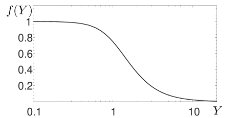
Figure 1: The function $f(Y)$.

The equation of state for a perfect gas yields:

$${{\bm{\nabla}}\rho\over\rho}={{\bm{\nabla}}P\over P}-{{\bm{\nabla}}T\over T},$$ (16)

where $P$ and $T$ are the mean fluid pressure and temperature, respectively. We assume for simplicity that the gradient of the mean fluid pressure vanishes, ${\bm{\nabla}}P=0$. In this case Eq. (14) can be rewritten in the following form:

$${\bm{V}}^{\rm eff}=-A\,D_{T}\,f\left[\big{(}B\,\delta_{{}_{T}}\big{)}^{2/3}\right]\,{{\bm{\nabla}}T\over T},$$ (17)

where the dimensionless parameter $\delta_{{}_{T}}$ is defined as

$$\delta_{{}_{T}}=\ell_{0}{|\mbox{\boldmath$\nabla$}T|\over T}.$$ (18)

It follows from Eq. (17) that for a weak stratification, $B\,\delta_{{}_{T}}\ll 1$, the effective particle velocity is given by the following expression:

$${\bm{V}}^{\rm eff}=-A\,D_{T}\,\left[1-{1\over 4}\left(B\,\delta_{{}_{T}}\right)^{2/3}\right]\,{{\bm{\nabla}}T\over T},$$ (19)

while for a strong stratification, $B\,\delta_{{}_{T}}\gg 1$, the effective particle velocity is given by the following formula:

$${\bm{V}}^{\rm eff}=-{4\pi A\,D_{T}\,\over 3^{3/2}}\,\left(B\,\delta_{{}_{T}}\right)^{-4/3}\,{{\bm{\nabla}}T\over T}.$$ (20)

To determine the function $A$, we compare Eq. (19) with Eq. (9) for the particle effective velocity, ${\bm{V}}^{\rm eff}$, derived for a small Stokes number, ${\rm St}\ll 1$, and a weak stratification, $\delta_{{}_{T}}\ll 1$ (see EKR96 ; EKR97 ; EKR00 ; EKRS00 ; EKRS01 ; EKR13 ). This comparison shows that $A=\alpha$, where the function $\alpha$ is determined by Eq. (10). Therefore, the expression for the effective particle velocity can be written as follows:

$${\bm{V}}^{\rm eff} = -{2D_{T}\,\alpha\over\sqrt{3}\,\big{(}B\,\delta_{{}_{T}}\big{)}^{4/3}}\,\biggl{[}{\pi\over 6}+\arctan\biggl{(}{2\big{(}B\,\delta_{{}_{T}}\big{)}^{2/3}-1\over\sqrt{3}}\biggr{)}$$ (21)

$$-{\sqrt{3}\over 6}\,\ln{\left[1+\big{(}B\,\delta_{{}_{T}}\big{)}^{2/3}\right]^{3}\over 1+\big{(}B\,\delta_{{}_{T}}\big{)}^{2}}\biggr{]}\,{{\bm{\nabla}}T\over T},$$

where we used Eq. (15). To determine the second function $B$, we assume that

$$B=\alpha^{\beta}\,\varphi({\rm St},{\rm Re}),$$ (22)

where the exponent $\beta$ should be larger than $3/4$. Indeed, when St $\to\infty$, the effective velocity should vanish, that occurs when $\beta>3/4$ [see Eq. (20)]. We will see in the next section that a good agreement of the results of laboratory experiments with the theoretical results is achieved when $\beta=1$ (see Sect. III.4). The ratio $B/\alpha$ is a free parameter in the theory to be determined in our laboratory experiments and atmospheric observations (see Sect. IV).

The effective velocity $V^{\rm eff}$ versus the particle diameter $d$ for conditions pertinent to our laboratory experiments and the atmospheric turbulence is shown in Fig. 2. Note that the characteristic Reynolds numbers based on the turbulent integral scale in the atmospheric turbulence vary from $10^{6}$ to $10^{7}$, and in our laboratory experiments the Reynolds numbers vary from $10^{2}$ to $10^{3}$. It follows from Fig. 2 that the ratio of the effective velocity of inertial particles to the characteristic vertical turbulent velocity for large Reynolds numbers is less than 1.

III.3 Turbulent diffusion of inertial particles

Equation (12) also allows us to determine the turbulent diffusion tensor for particles:

$$D_{ij}^{T}=\int\tau(k)\langle v_{i}({\bm{k}})\,v_{j}(-{\bm{k}})\rangle\,d{\bm{k}}.$$ (23)

Using Eqs. (B)-(44) given in Appendix B, we obtain:

$$D_{ij}^{T} = {3D_{T}\over 2}\,\biggl{\{}\delta_{ij}\,\left[1-{2\over 3}f\left[\big{(}B\,\delta_{{}_{T}}\big{)}^{2/3}\right]\right]$$ (24)

$$-{\lambda_{i}\,\lambda_{j}\over\lambda^{2}}\,\biggl{[}1-2f\left[\big{(}B\,\delta_{{}_{T}}\big{)}^{2/3}\right]\biggr{]}\biggr{\}}.$$

It follows from Eq. (24) that for a weak stratification, $B\,\delta_{{}_{T}}\ll 1$, the turbulent diffusion tensor for particles is given by the following expression:

$$D_{ij}^{T} = {D_{T}\over 2}\,\biggl{[}\delta_{ij}+3{\lambda_{i}\,\lambda_{j}\over\lambda^{2}}$$ (25)

$$+{1\over 2}\,\left(\delta_{ij}-3{\lambda_{i}\,\lambda_{j}\over\lambda^{2}}\right)\,\left(B\,\delta_{{}_{T}}\right)^{2/3}\biggr{]},$$

while for a strong stratification, $B\,\delta_{{}_{T}}\gg 1$, it is given by the following formula:

$$D_{ij}^{T} = {3D_{T}\over 2}\,\biggl{[}\delta_{ij}-{\lambda_{i}\,\lambda_{j}\over\lambda^{2}}$$ (26)

$$+{8\pi\over 3^{5/2}}\,\left(\delta_{ij}-3{\lambda_{i}\,\lambda_{j}\over\lambda^{2}}\right)\,\left(B\,\delta_{{}_{T}}\right)^{-4/3}\biggr{]}.$$

Equations (24)-(26) show that turbulent diffusion tensor for particles is anisotropic for stratified turbulence.

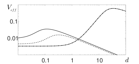
Figure 2: Effective velocity $V^{\rm eff}$ measured in the units of the r.m.s turbulent vertical velocity, $u_{z}^{(\rm rms)}$, versus the particle diameter $d$ ($\mu$m) for atmospheric conditions where the parameter $B/\alpha=1$ (dashed-dotted) and for laboratory experiments conditions: the oscillating grid turbulence where the parameter $B/\alpha=30$ (solid) and the multi-fan produced turbulence where the parameter $B/\alpha=18$ (dashed).

III.4 Effective coefficient of turbulent thermal diffusion

An equation for the mean number density, $N$, of inertial particles reads:

$${\partial N\over\partial t}+{\bm{\nabla}}{\bf\cdot}\,\left[N\,({\bm{W}}_{g}+{\bm{V}}^{\rm eff})-(D+D_{T})\,{\bm{\nabla}}N\right]=0,$$

(27)

(see (EKR96, ; EKR97, ; EKR98, ; EKR00, ; EKRS00, ; EKRS01, )), where we took into account the effect of gravity for inertial particles and molecular Brownian diffusion. However, for simplicity we neglected the effects of stratification and particle inertia on the particle turbulent diffusion coefficient. The steady state solution of Eq. (27) reads:

$${{\bm{\nabla}}N\over N}={{\bm{W}}_{g}+{\bm{V}}^{\rm eff}\over D+D_{T}}.$$ (28)

This implies that the dimensionless parameter, $\delta_{{}_{N}}\equiv\ell_{0}|\mbox{\boldmath$\nabla$}N|/N$, characterising variations of the mean particle number density, is given by the following formula:

$$\delta_{{}_{N}}={\ell_{0}\over 1+D/D_{T}}\left|\alpha\,f\left[\big{(}B\,\delta_{{}_{T}}\big{)}^{2/3}\right]\,{{\bm{\nabla}}T\over T}-{\tau_{p}{\bm{g}}\over D_{T}}\right|.$$ (29)

When the gradient of the mean temperature, $\mbox{\boldmath$\nabla$}T$, is directed along (or opposite to) the vertical direction, Eq. (29) yields the following ratio:

$${\alpha^{\rm eff}\over\alpha} = {1\over 1+D/D_{T}}\biggl{|}f\left[\big{(}B\,\delta_{{}_{T}}\big{)}^{2/3}\right]$$ (30)

$$+{\tau_{p}\,g\,\ell_{0}\over\alpha\,\delta_{{}_{T}}\,D_{T}}\,{\rm sgn}(\nabla_{z}T)\biggr{|},$$

where we introduced a new parameter $\alpha^{\rm eff}\equiv\delta_{{}_{N}}/\delta_{{}_{T}}$. It follows from Eq. (30) that for a weak stratification, $B\,\delta_{{}_{T}}\ll 1$, the ratio $\alpha^{\rm eff}/\alpha$ is given by the following formula:

$${\alpha^{\rm eff}\over\alpha} = {1\over 1+D/D_{T}}\biggl{|}1-{1\over 4}\left(B\,\delta_{{}_{T}}\right)^{2/3}$$ (31)

$$+{\tau_{p}\,g\,\ell_{0}\over\alpha\,\delta_{{}_{T}}\,D_{T}}\,{\rm sgn}(\nabla_{z}T)\biggr{|},$$

while for a strong stratification, $B\,\delta_{{}_{T}}\gg 1$, it is given by the following expression:

$${\alpha^{\rm eff}\over\alpha} = {1\over 1+D/D_{T}}\biggl{|}{4\pi\over 3^{3/2}}\,\left(B\,\delta_{{}_{T}}\right)^{-4/3}$$ (32)

$$+{\tau_{p}\,g\,\ell_{0}\over\alpha\,\delta_{{}_{T}}\,D_{T}}\,{\rm sgn}(\nabla_{z}T)\biggr{|}.$$

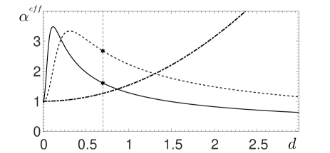
Figure 3: Dependencies of the effective turbulent thermal diffusion coefficient $\alpha^{\rm eff}$ versus the particle diameter $d$ ($\mu$m) for atmospheric conditions where the parameter $B/\alpha=1$ (dashed-dotted), and for laboratory experiments with oscillating grid turbulence where the parameter $B/\alpha=30$ (solid), and multi-fan produced turbulence where the parameter $B/\alpha=18$ (dashed). Vertical line corresponds to the particle diameter $d=0.7$ $\mu$m used in the experiments (stars are values obtained from measurements).

The dependencies of the effective turbulent thermal diffusion coefficient $\alpha^{\rm eff}$ versus the particle diameter $d$ for conditions pertinent for atmospheric turbulence and laboratory experiments are shown in Fig. 3. To isolate turbulent thermal diffusion from other effects hereafter we do not take into account the gravity effect. Inspection of Fig. 3 shows that for the conditions pertinent for our laboratory experiments the effective turbulent thermal diffusion coefficient $\alpha^{\rm eff}$ increases for very small particle size $d$, reaches the maximum at small $d$ and slowly decreases for larger particle size. In the atmospheric turbulence the effective turbulent thermal diffusion coefficient $\alpha^{\rm eff}$ behaves in a similar way, except for $\alpha^{\rm eff}$ reaches the maximum at much larger particle size $d$.

IV Validation of theory in laboratory experiments and atmospheric turbulence

To validate the theory of turbulent thermal diffusion in strongly stratified turbulent flows we perform laboratory experiments in different set-ups: in the oscillating grid turbulence (see, e.g., BEE04 ; EEKR04 ; EEKMR06 ; EKR10 ; EEKR11 ; EEKR13 ) and in the multi-fan produced turbulence (see, e.g., EEKR06 ). We also validate the theory of turbulent thermal diffusion against data of meteorological observations (see, e.g., SSEKR09 ).

IV.1 Particles in the oscillating grid turbulence

In this section we describe very briefly the experimental set-up and measurement facilities in the oscillating grid turbulence. The details of the experimental set-up and measurements in the oscillating grid turbulence can be found in EEKMR06 ; EKR10 ; EEKR11 ; EEKR13 . The experiments in stratified turbulence have been conducted in rectangular chamber with dimensions $26\times 58\times 26$ cm³ in air flow. In the experiments turbulence is produced by two oscillating vertically oriented grids with bars arranged in a square array. The grids are parallel to the side walls and positioned at a distance of two grid meshes from the chamber walls. They are operated at the same amplitude, at a random phase and at the same frequency up to $10.5$ Hz.

A vertical mean temperature gradient in the turbulent air flow was formed by attaching two aluminium heat exchangers to the bottom and top walls of the test section which allowed us to form a mean temperature gradient up to 1.15 K/cm at a mean temperature of about 308 K when the frequency of the grid oscillations $f=10.5$ Hz. To improve heat transfer in the boundary layers at the bottom and top walls we used heat exchangers with rectangular fins $0.3\times 0.3\times 1.5$ cm³. The temperature field was measured with a temperature probe equipped with a vertical array of 12 E-thermocouples in the central part of the chamber in many locations.

The velocity fields were measured using a Stereoscopic Particle Image Velocimetry (PIV) with LaVision Flow Master III system. We obtain velocity maps in the central region of the flow in the cross-section perpendicular to the grids and parallel to a front view plane. An incense smoke with sub-micron particles ($\rho_{p}/\rho\sim 10^{3})$, was used as a tracer for the PIV measurements. Smoke was produced by high temperature sublimation of solid incense grains. These particles have an approximately spherical shape and the mean diameter of 0.7 $\mu$m.

We determined the mean and the r.m.s. velocities, two-point correlation functions and an integral scale of turbulence from the measured velocity fields. Series of 520 pairs of images acquired with a frequency of 2 Hz, were stored for calculating velocity maps and for ensemble and spatial averaging of turbulence characteristics. We measured velocity in a flow domain $32.8\times 24.8$ cm² with a spatial resolution of $0.24$ mm/pixel. The mean and r.m.s. velocities for every point of a velocity map were calculated by averaging over 520 independent velocity maps, and then they were spatially averaged over the central flow region. An integral scale of turbulence, $\ell$, was determined from the two-point correlation functions of the velocity field. The characteristic turbulence time in the experiments is much smaller than the time during which the velocity fields are measured $(260$ s). We performed experiments for different temperature difference, $\Delta T$, between the top and bottom plates.

Spatial distributions for 0.7 $\mu$m and 10 $\mu$m particles were determined by Particle Image Velocimetry (PIV) system using the effect of Mie light scattering by particles in the flow BEE04 ; EEKR04 ; EEKMR06 . In order to characterize the spatial distribution of particle number density in the non-isothermal flow, the distribution of the scattered light intensity measured in the isothermal case was used for the normalization of the scattered light intensity obtained in a non-isothermal flow under the same conditions. The scattered light intensities in each experiment were also normalized by corresponding scattered light intensities averaged over the vertical coordinate.

For experimental study of turbulent thermal diffusion of inertial particles we used borosilicate hollow glass particles having an approximately spherical shape, a mean diameter of $10\,\mu$m and the material density $\rho_{p}\approx 1.4$ g/cm³. These particles have been injected in the chamber using an air jet in order to improve particle mixing and prevent from particle agglomeration. We used a custom-made acoustic feeding device for injecting particles into the flow comprising an acrylic glass chamber with a size of 9 $\times$ 9 $\times$ 4 cm³. Two plastic slabs inside the chamber are used as air guides to achieve optimal flow with entrained particles. Particle dispensation zone (a disk of 25 mm diameter and 5 mm thickness) is located at the bottom of the chamber. A standard woofer (oval 2 $\times$ 3.5”) at a frequency of 220 Hz sways a latex membrane on which particles are loaded. A cylindrical cavity is used to contain the particles on the latex membrane. The batch of particles on the membrane should roughly fill the cavity. When the membrane vibrates, particles are entrained into air. Particle feeding device has a pressurized air inlet with a bellow having a 8 mm diameter tube with standard quick release connector. The entrained particles leave the chamber with a stream of air through the outlet.

The parameters in the oscillating grid turbulence are as follows: the integral length scales in the vertical and horizontal directions are $\ell_{z}=1.4$ cm and $\ell_{y}=2.2$ cm; the characteristic turbulent vertical and horizontal velocities (the root mean square velocity) are $u_{z}=7.8$ cm s^-1 and $u_{y}=17.3$ cm s^-1; the characteristic turbulent times in these directions are $\tau_{z}=0.18$ s and $\tau_{y}=0.13$ s; the vertical and horizontal Reynolds numbers are Re${}_{z}\equiv\ell_{z}u_{z}/\nu=73$ and Re${}_{y}\equiv\ell_{y}u_{y}/\nu=254$.

In Fig. 4 we show the effective turbulent thermal diffusion coefficient $\alpha^{\rm eff}$ versus the parameter $\delta_{{}_{T}}$ for 0.7 $\mu$m particles with the parameter $B/\alpha=21$ and for 10 $\mu$m particles with the parameter $B/\alpha=18$. The laboratory experiments with oscillating grid turbulence are performed with 0.7 $\mu$m particles and 10 $\mu$m particles for different temperature difference $\Delta T$ between the top and bottom heat exchangers. For comparison we also show in Fig. 4 the function $\alpha^{\rm eff}(\delta_{{}_{T}})$ for atmospheric turbulence for 1 $\mu$m particles, where the parameter $B/\alpha=1$. The measured values of $\alpha^{\rm eff}$ are in a good agreement with theoretical predictions.

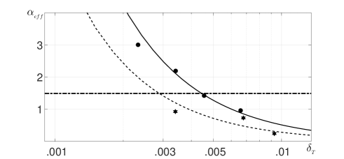
Figure 4: Effective turbulent thermal diffusion coefficient $\alpha^{\rm eff}$ versus the parameter $\delta_{{}_{T}}$ for 0.7 $\mu$m particles with the parameter $B/\alpha=21$ (solid) and for 10 $\mu$m particles with the parameter $B/\alpha=18$ (dashed). The laboratory experiments with oscillating grid turbulence are performed with 0.7 $\mu$m particles (circle) and 10 $\mu$m particles (star) for different temperature difference $\Delta T$ between the top and bottom heat exchangers. For comparison the function $\alpha^{\rm eff}(\delta_{{}_{T}})$ is also shown for atmospheric turbulence (dashed-dotted) for 1 $\mu$m particles and the parameter $B/\alpha=1$.

IV.2 Particles in the multi-fan produced turbulence

In this section we describe very briefly the experimental set-up and measurement facilities in the multi-fan produced turbulence. The details of the experimental set-up and measurements in the multi-fan produced turbulence can be found in EEKR06 . Experiments were conducted in a multi-fan turbulence generator that is the perspex cube box with dimensions $40\times 40\times 40$ cm³. It includes eight fans with rotation frequency of up to 2800 rpm mounted in the corners of the box and facing the center of the box.

At the top and bottom walls of the Perspex box two heat exchangers with rectangular $0.3\times 0.3\times 1.5$ cm³ fins were installed to improve heat transfer in the boundary layers at the bottom and top walls. The upper wall was heated up to 343 K, the bottom wall was cooled to 283 K. Two additional fans were installed at the bottom and top walls of the chamber in order to produce a large mean temperature gradient $(\sim 0.92$ K/cm) in the core of the flow. The temperature was measured with a high-frequency response thermocouple which was glued externally to a wire. Velocity fields and particle spatial distribution were determined using digital Particle Image Velocimetry (PIV) system (see previous subsection). The laboratory experiments with the multi-fan produced turbulence are performed with 0.7 $\mu$m particles for $\Delta T=50$ K.

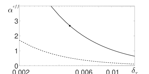
Figure 5: Effective turbulent thermal diffusion coefficient $\alpha^{\rm eff}$ versus the parameter $\delta_{{}_{T}}$ for 0.7 $\mu$m particles (solid) and for 10 $\mu$m particles (dashed) for the parameter $B/\alpha=18$. The laboratory experiments with the multi-fan produced turbulence are performed with 0.7 $\mu$m particles for the temperature difference $\Delta T=50$ K between the top and bottom heat exchangers (square).

The parameters of the multi-fan produced turbulence are as follows: the integral length scales in the vertical and horizontal directions are $\ell_{z}=1.64$ cm and $\ell_{y}=1.49$ cm; the characteristic turbulent vertical and horizontal velocities (the root mean square velocity) are $u_{z}=80$ cm s^-1 and $u_{y}=71$ cm s^-1; the characteristic turbulent times in these directions are $\tau_{z}=2.05\times 10^{-2}$ s and $\tau_{y}=2.1\times 10^{-2}$ s; the vertical and horizontal Reynolds numbers are Re${}_{z}\equiv\ell_{z}u_{z}/\nu=875$ and Re${}_{y}\equiv\ell_{y}u_{y}/\nu=705$.

Unfortunately, the region of isotropic and homogeneous turbulence in the multi-fan produced turbulence is not large. The presence of 10 fans in this set-up does not allow us to perform velocity and temperature measurements, and to obtain spatial profiles of particle number density in many locations. This is a reason why we performed only several experiments in the multi-fan produced turbulence.

In Fig. 5 we show the effective turbulent thermal diffusion coefficient $\alpha^{\rm eff}$ versus the parameter $\delta_{{}_{T}}$ for 0.7 $\mu$m particles (solid line) and for 10 $\mu$m particles (dashed line) for the parameter $B/\alpha=18$. The measured value of $\alpha^{\rm eff}$ is in an agreement with theoretical predictions.

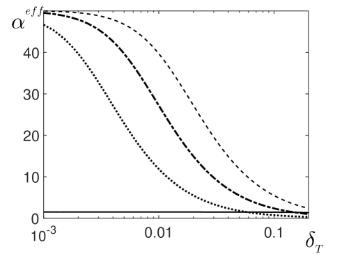
Figure 6: Effective turbulent thermal diffusion coefficient $\alpha^{\rm eff}$ versus the parameter $\delta_{{}_{T}}$ for 1 $\mu$m particles and $B/\alpha=1$ (solid) and for 10 $\mu$m particles and different values of the parameter $B/\alpha$: $\;B/\alpha=1$ (dashed), $B/\alpha=2$ (dashed-dotted), $B/\alpha=5$ (dotted), and other parameters corresponds to the atmospheric turbulence conditions.

IV.3 Particles in the atmospheric turbulence

Tropopause in the atmosphere is a well-known region with strong gradients of temperature and also with substantial amount of aerosol particles, which remain there over long time (see, e.g., BS05 ). The theory of turbulent thermal diffusion for small temperature stratifications and small Stokes numbers has been previously applied in SSEKR09 to the GOMOS (Global Ozone Monitoring by Occultation of Stars) aerosol observations near the tropopause in order to explain the shape of aerosol vertical profiles with elevated concentrations located almost symmetrically with respect to temperature profile. The altitude of the GOMOS measurements is in the range from 5 km to 20 km. Analysis of data of simultaneous observations of the vertically-resolved aerosol concentrations and mean temperature in the vicinity of the tropopause shows that the aerosol concentration and temperature profiles are often anti-correlated SSEKR09 . These observations are explained using the effect of turbulent thermal diffusion, where the turbulent flux of particles is directed towards to the mean temperature minimum.

In Fig. 6 we show the effective turbulent thermal diffusion coefficient $\alpha^{\rm eff}$ obtained from the generalized theory versus the parameter $\delta_{{}_{T}}$ for 1 $\mu$m particles and $B/\alpha=1$, and for 10 $\mu$m particles and different values of the parameter $B/\alpha$. It is seen in Fig. 6 that $\alpha^{\rm eff}$ depends strongly on the particle size. Note that in the atmospheric turbulent flows the parameter $\delta_{{}_{T}}$ varies in the range from $10^{-3}$ to $10^{-2}$ (see, e.g., SSEKR09 ). This implies that $\alpha^{\rm eff}/\alpha$ is of the order of 1 in this range of the mean temperature variations. For example, for aerosols having the diameter of 1-3 $\mu$m, the coefficient $\alpha^{\rm eff}\approx\alpha$ exceeds 1 when the turbulent diffusion coefficient $D_{T}\sim 10^{4}$ cm² s^-1 or less. This is in agreement with the data obtained from the GOMOS aerosol observations near the tropopause SSEKR09 .

V Discussion and conclusions

In the present study we have investigated turbulent thermal diffusion of small inertial particles in the temperature stratified turbulence. This effect results in the appearance of a non-diffusive turbulent flux of particles directed towards the turbulent heat flux.

The theory of turbulent thermal diffusion has been previously developed only for small temperature gradients and small Stokes numbers (EKR96, ; EKR97, ; EKR00, ; EKRS00, ; EKRS01, ; PM02, ; RE05, ). In the present study we have generalized the theory of turbulent thermal diffusion for arbitrary temperature gradients and Stokes numbers. We have also performed laboratory experiments in the oscillating grid turbulence and in the multi-fan produced turbulence to validate the theory of turbulent thermal diffusion in strongly stratified turbulent flows.

Turbulent flux of inertial particles caused by turbulent thermal diffusion is proportional to the product of the effective velocity of inertial particles and the mean particle number density. We have shown that the ratio of the effective velocity of inertial particles to the characteristic vertical turbulent velocity for large Reynolds numbers is less than 1. We demonstrated that the effective velocity of inertial particles increases with the increase of the Stokes numbers, reaches the maximum at small Stokes numbers and decreases for larger Stokes numbers. In the laboratory experiments the effective velocity of inertial particles reaches the maximum at St $=10^{-4}$, while for the atmospheric turbulence it reaches the maximum at St $=0.05$. The effective coefficient of turbulent thermal diffusion decreases with the mean temperature gradient. For very large Reynolds numbers this dependence on the mean temperature gradient is very weak. The obtained results of the laboratory experiments are in a good agreement with the theoretical predictions. However, the results obtained in our laboratory experiments clearly indicate the difficulty associated with the experimental observation of the phenomenon of turbulent thermal diffusion, i.e., this effect is quite strong only in a certain range of values of Stokes number, flow Reynolds number and temperature gradient.

Appendix A Model of turbulent velocity field

The anelastic condition div ${\bm{u}}={\bm{u}}\cdot{\bm{\lambda}}$ in the ${\bf k}$-space implies that $k_{1}^{(i)}\langle u_{i}({\bm{k}}_{1})\,u_{j}({\bm{k}}_{2})\rangle=0$ and $k_{2}^{(j)}\langle u_{i}({\bm{k}}_{1})\,u_{j}({\bm{k}}_{2})\rangle=0$, where $k_{1}^{(i)}=k_{i}+i\lambda_{i}$ and $k_{2}^{(i)}=-k_{i}+i\lambda_{i}$. We consider the model of the turbulent velocity field in the following form:

$$\langle u_{i}({\bm{k}}_{1})\,u_{j}({\bm{k}}_{2})\rangle=-\langle{\bm{u}}^{2}\rangle\,\Phi(k)\,\biggl{[}\delta_{ij}\left({\bm{k}}_{1}\cdot{\bm{k}}_{2}\right)-k_{1}^{(i)}\,k_{2}^{(j)}\biggr{]},$$

(33)

where ${\bm{k}}_{1}\cdot{\bm{k}}_{2}=-(k^{2}+\lambda^{2})$ and $k_{1}^{(i)}\,k_{2}^{(j)}=-(k_{i}\,k_{j}-i\lambda_{i}\,k_{j}+i\lambda_{j}\,k_{i}+\lambda_{i}\,\lambda_{j})$, so that

$$\langle u_{i}({\bm{k}}_{1})\,u_{j}({\bm{k}}_{2})\rangle=\langle{\bm{u}}^{2}\rangle\,\Phi(k)\,k^{2}\biggl{[}\delta_{ij}-{k_{i}\,k_{j}\over k^{2}}+{i\over k^{2}}\,\big{(}\lambda_{i}\,k_{j}$$

$$\quad-\lambda_{j}\,k_{i}\big{)}+{\lambda^{2}\over k^{2}}\left(\delta_{ij}-{\lambda_{i}\,\lambda_{j}\over\lambda^{2}}\right)\biggr{]}.$$ (34)

Here $\Phi(k)$ is unknown function to be determined below. Integrating the correlation function $\langle u_{i}({\bm{k}}_{1})\,u_{i}({\bm{k}}_{2})\rangle$ over ${\bm{k}}$ we obtain

$$\int\langle u_{i}({\bm{k}}_{1})\,u_{i}({\bm{k}}_{2})\rangle\,d{\bm{k}}=2\langle{\bm{u}}^{2}\rangle\,\int\Phi(k)\,(k^{2}+\lambda^{2})\,d{\bm{k}}$$

$$=8\pi\langle{\bm{u}}^{2}\rangle\,\int\Phi(k)\,(k^{2}+\lambda^{2})\,k^{2}\,dk.$$ (35)

On the other hand,

$$\int\langle u_{i}({\bm{k}}_{1})\,u_{i}({\bm{k}}_{2})\rangle\,d{\bm{k}}\equiv\langle{\bm{u}}^{2}\rangle\int E(k)\,k^{2}\,dk,$$ (36)

where $E(k)$ is the spectrum function of the turbulent velocity field. Comparing Eqs. (35) and (36), we obtain the function $\Phi(k)$:

$$\Phi(k)={E(k)\over 8\pi(k^{2}+\lambda^{2})}.$$ (37)

Substituting this function into Eq. (33), we obtain Eq. (11).

Appendix B Derivation of equation for the effective velocity

In this Appendix we derive equation for the effective velocity of particles. Using Eqs. (12) and (13), we obtain:

$${\bm{V}}^{\rm eff} = -\langle\tau{\bm{v}}\,{\rm div}{\bm{v}}\rangle=i\int\tau(k)\,k_{j}\langle v_{i}({\bm{k}})\,v_{j}(-{\bm{k}})\rangle\,d{\bm{k}}$$ (38)

$$= -2D_{T}A\mbox{\boldmath$\lambda$}\int_{0}^{1}{\bar{\tau}\,d\bar{\tau}\over 1+a\bar{\tau}^{3}},$$

where $a=(B\,\ell_{0}\lambda)^{2}$, $\ell_{0}=k_{0}^{-1}$ and $\tau(k)=2\tau_{0}\bar{\tau}(k)$. For the integration over angles in ${\bm{k}}$-space in Eq. (38) we used the following integrals:

$$\int_{0}^{2\pi}\,d\varphi\int_{0}^{\pi}\sin\vartheta\,d\vartheta=4\pi.$$ (39)

$$\int_{0}^{2\pi}\,d\varphi\int_{0}^{\pi}\sin\vartheta\,d\vartheta\,{k_{i}\,k_{j}\over k^{2}}={4\pi\over 3}\,\delta_{ij}.$$ (40)

Now let us calculate the integral over $\bar{\tau}$ in Eq. (38):

$$f(a) = 2\int_{0}^{1}{\bar{\tau}\,d\bar{\tau}\over 1+a\bar{\tau}^{3}}={2\over a^{2/3}}\,\int_{0}^{a^{1/3}}{X\,dX\over 1+X^{3}}$$

$$= {2\over a^{2/3}}\,\left[\int_{0}^{a^{1/3}}{\,dX\over 1-X+X^{2}}-\int_{0}^{a^{1/3}}{\,dX\over 1+X^{3}}\right],$$

where $X=a^{1/3}\bar{\tau}$, and

$$\int{\,dX\over 1+X^{3}}={1\over 6}\ln{(1+X)^{3}\over 1+X^{3}}+{1\over\sqrt{3}}\arctan{2X-1\over\sqrt{3}},$$

(42)

$$\int{\,dX\over 1-X+X^{2}}={2\over\sqrt{3}}\arctan{2X-1\over\sqrt{3}}.$$ (43)

Substituting Eqs. (42) and (43) into Eq. (B) we obtain the expression for the function $f(a)$:

$$f(a) = {2\over\sqrt{3}\,a^{2/3}}\,\biggl{[}{\pi\over 6}+\arctan\left({2a^{1/3}-1\over\sqrt{3}}\right)$$ (44)

$$-{\sqrt{3}\over 6}\,\ln{\left(1+a^{1/3}\right)^{3}\over 1+a}\biggr{]}.$$

Therefore, the effective velocity of particles caused by turbulent thermal diffusion is ${\bm{V}}^{\rm eff}=-A\,D_{T}\,f\left[(B\,\ell_{0}\lambda)^{2}\right]\,\mbox{\boldmath$\lambda$}$.

References

- (1) G. T. Csanady, Turbulent Diffusion in the Environment (Reidel, Dordrecht, 1980).
- (2) Ya. B. Zeldovich, A. A. Ruzmaikin, and D. D. Sokoloff, The Almighty Chance (Word Scientific Publ., Singapore, 1990).
- (3) A. K. Blackadar, Turbulence and Diffusion in the Atmosphere (Springer, Berlin, 1997).
- (4) J. H. Seinfeld and S. N. Pandis, Atmospheric Chemistry and Physics. From Air Pollution to Climate Change., 2nd ed. (John Wiley & Sons, NY, 2006).
- (5) L. I. Zaichik, V. M. Alipchenkov, and E. G. Sinaiski, Particles in turbulent flows (John Wiley & Sons, NY, 2008).
- (6) C. T. Crowe, J. D. Schwarzkopf, M. Sommerfeld and Y. Tsuji, Multiphase flows with droplets and particles, second edition (CRC Press LLC, NY, 2011).
- (7) P. J. Armitage, Astrophysics of Planet Formation (Cam- bridge University Press, Cambridge, UK, 2010).
- (8) Z. Warhaft, Passive scalars in turbulent flows, Annu. Rev. Fluid Mech. 32, 203 (2000).
- (9) R. A. Shaw, Particle-turbulence interactions in atmospheric clouds, Annu. Rev. Fluid Mech. 35, 183 (2003).
- (10) A. Khain, M. Pinsky, T. Elperin, N. Kleeorin, I. Rogachevskii and A. Kostinski, Critical comments to results of investigations of drop collisions in turbulent clouds, Atmosph. Res. 86, 1 (2007).
- (11) Z. Warhaft, Laboratory studies of droplets in turbulence: towards understanding the formation of clouds, Fluid Dyn. Res. 41, 011201 (2009).
- (12) F. Toschi and E. Bodenschatz, Lagrangian properties of particles in turbulence, Annu. Rev. Fluid Mech. 41, 375 (2009).
- (13) S. Balachandar and J. K. Eaton, Turbulent dispersed multiphase flow, Annu. Rev. Fluid Mech. 42, 111 (2010).
- (14) M. Caporaloni, F. Tampieri, F. Trombetti and O. Vittori, Transfer of particles in nonisotropic air turbulence, J. Atmosph. Sci. 32, 565 (1975).
- (15) M. Reeks, The transport of discrete particle in inhomogeneous turbulence, J. Aerosol Sci. 14, 729 (1983).
- (16) A. Guha, A unified Eulerian theory of turbulent deposition to smooth and rough surfaces, J. Aerosol Sci. 28, 1517 (1997).
- (17) T. Elperin, N. Kleeorin and I. Rogachevskii, Formation of inhomogeneities in two-phase low-Mach-number compressible turbulent fluid flows, Int. J. Multiphase Flow 24, 1163 (1998).
- (18) A. Guha, Transport and deposition of particles in turbulent and laminar flow, Annu. Rev. Fluid Mech. 40, 311 (2008).
- (19) Dh. Mitra, N. E. L. Haugen and I. Rogachevskii, Turbophoresis in forced inhomogeneous turbulence, Phys. Rev. Fluids, submitted; arXiv:1603.00703.
- (20) T. Elperin, N. Kleeorin and I. Rogachevskii, Turbulent thermal diffusion of small inertial particles, Phys. Rev. Lett. 76, 224 (1996).
- (21) T. Elperin, N. Kleeorin and I. Rogachevskii, Turbulent barodiffusion, turbulent thermal diffusion and large-scale instability in gases, Phys. Rev. E 55, 2713 (1997).
- (22) T. Elperin, N. Kleeorin and I. Rogachevskii, Mechanisms of formation of aerosol and gaseous inhomogeneities in the turbulent atmosphere, Atmosph. Res. 53, 117 (2000).
- (23) T. Elperin, N. Kleeorin, I. Rogachevskii and D. Sokoloff, Passive scalar transport in a random flow with a finite renewal time: Mean-field equations, Phys. Rev. E 61, 2617 (2000).
- (24) T. Elperin, N. Kleeorin, I. Rogachevskii and D. Sokoloff, Mean-field theory for a passive scalar advected by a turbulent velocity field with a random renewal time, Phys. Rev. E 64, 026304 (2001).
- (25) R. V. R. Pandya and F. Mashayek, Turbulent thermal diffusion and barodiffusion of passive scalar and dispersed phase of particles in turbulent flows, Phys. Rev. Lett. 88, 044501 (2002).
- (26) M. W. Reeks, On model equations for particle dispersion in inhomogeneous turbulence, Int. J. Multiph. Flow 31, 93 (2005).
- (27) J. Buchholz, A. Eidelman, T. Elperin, G. Grünefeld, N. Kleeorin, A. Krein, I. Rogachevskii, Experimental study of turbulent thermal diffusion in oscillating grids turbulence, Experim. Fluids 36, 879 (2004).
- (28) A. Eidelman, T. Elperin, N. Kleeorin, A. Krein, I. Rogachevskii, J. Buchholz, and G. Grünefeld, Turbulent thermal diffusion of aerosols in geophysics and in laboratory experiments, Nonl. Proc. Geophys. 11, 343 (2004).
- (29) A. Eidelman, T. Elperin, N. Kleeorin, A. Markovich, I. Rogachevskii, Experimental detection of turbulent thermal diffusion of aerosols in non-isothermal flows, Nonl. Proc. Geophys. 13, 109 (2006).
- (30) A. Eidelman, T. Elperin, N. Kleeorin, I. Rogachevskii and I. Sapir-Katiraie, Turbulent thermal diffusion in a multi-fan turbulence generator with the imposed mean temperature gradient, Experim. Fluids 40, 744 (2006).
- (31) N. E. L. Haugen, N. Kleeorin, I. Rogachevskii and A. Brandenburg, Detection of turbulent thermal diffusion of particles in numerical simulations, Phys. Fluids 24, 075106 (2012).
- (32) M. Sofiev, V. Sofieva, T. Elperin, N. Kleeorin, I. Rogachevskii and S. S. Zilitinkevich, Turbulent diffusion and turbulent thermal diffusion of aerosols in stratified atmospheric flows, J. Geophys. Res. 114, D18209 (2009).
- (33) A. Hubbard, Turbulent thermal diffusion: a way to concentrate dust in protoplanetary discs, Monthly Notes Roy. Astron. Soc. 456, 3079-3089 (2016).
- (34) M. R. Maxey, The gravitational settling of aerosol particles in homogeneous turbulence and random flow field, J. Fluid Mech. 174, 441 (1987).
- (35) S. Chandrasekhar, Stochastic problems in physics and astronomy, Rev. Modern Phys. 15, 1 (1943).
- (36) A. I. Akhiezer and S. V. Peletminsky, Methods of Statistical Physics (Pergamon, Oxford, 1981).
- (37) T. Elperin, N. Kleeorin, M. A. Liberman and I. Rogachevskii, Tangling clustering instability for small particles in temperature stratified turbulence, Phys. Fluids 25, 085104 (2013).
- (38) T. Elperin, N. Kleeorin and I. Rogachevskii, Dynamics of passive scalar in compressible turbulent flow: large-scale patterns and small-scale fluctuations, Phys. Rev. E 52, 2617 (1995).
- (39) A. Eidelman, T. Elperin, N. Kleeorin, B. Melnik and I. Rogachevskii, Tangling clustering of inertial particles in stably stratified turbulence, Phys. Rev. E 81, 056313 (2010).
- (40) M. Bukai, A. Eidelman, T. Elperin, N. Kleeorin, I. Rogachevskii and I. Sapir-Katiraie, Transition phenomena in unstably stratified turbulent flows, Phys. Rev. E 83, 036302 (2011).
- (41) A. Eidelman, T. Elperin, I. Gluzman, N. Kleeorin and I. Rogachevskii, Experimental study of temperature fluctuations in forced stably stratified turbulent flows, Phys. Fluids 25, 015111 (2013).
- (42) G. Brasseur and S. Solomon, Aeronomy of the Middle Atmosphere, 3rd edition (Springer, NY, 2005).