Wormholes leading to extra dimensions

K. A. Bronnikov^a,b,c,1 and M. V. Skvortsova^b,2

^a

VNIIMS, Ozyornaya ul. 46, Moscow 119361, Russia

^b

Peoples’ Friendship University of Russia, ul. Miklukho-Maklaya 6, Moscow 117198, Russia

^c

National Research Nuclear University “MEPhI” (Moscow Engineering Physics Institute), Moscow, Russia

In 6D general relativity with a scalar field as a source of gravity, a new type of static wormhole solutions is presented: such wormholes connect our universe with a small 2D extra subspace with a universe where this extra subspace is large, and the whole space-time is effectively 6-dimensional. We consider manifolds with the structure ${\mathbb{M}}_{0}\times{\mathbb{M}}_{1}\times{\mathbb{M}}_{2}$, where ${\mathbb{M}}_{0}$ is 2D Lorentzian space-time while each of ${\mathbb{M}}_{1,2}$ can be a 2-sphere or a 2-torus. After selecting possible asymptotic behaviors of the metric functions compatible with the field equations, we give two explicit examples of wormhole solutions with spherical symmetry in our space-time and toroidal extra dimensions. In one example, with a massless scalar field (it is a special case of a well-known more general solution), the extra dimensions have a large constant size at the “far end”; the other example contains a nonzero potential $V(\phi)$ which provides a 6D anti-de Sitter asymptotic, where all spatial dimensions are infinite.

1 Introduction

Multidimensional theories suggest a great variety of geometries, topologies and compactification schemes (for reviews see, e.g., [1–4] and references therein). However, there still emerge new ideas on how our 4D space-time may be inscribed in a multidimensional world. One recently suggested idea [5] is that of exchanging roles of different dimensions in different parts of space-time.

More specifically, considered was [5] a 6D static space-time of the form ${\mathbb{M}}={\mathbb{M}}_{0}\times{\mathbb{M}}_{1}\times{\mathbb{M}}_{2}$, where ${\mathbb{M}}_{0}$ is 2D Lorentzian space-time parametrized by time $t$ and a “radial” coordinate $x$ while ${\mathbb{M}}_{1,2}$ are two-spheres with radii $r_{1}(x)$ and $r_{2}(x)$. Moreover, as $x\to-\infty$, $r_{1}\to\infty$ (so that the 4D space-time ${\mathbb{M}}_{0}\times{\mathbb{M}}_{1}$ is asymptotically flat) while $r_{2}$ tends to a small constant value, and ${\mathbb{M}}_{2}$ is thus a spherical extra space. The same picture occurs in the other asymptotic region, $x\to+\infty$, but, on the contrary, ${\mathbb{M}}_{1}$ is small and ${\mathbb{M}}_{2}$ is large, and now ${\mathbb{M}}_{0}\times{\mathbb{M}}_{2}$ is asymptotically flat. The spatial section of ${\mathbb{M}}_{0}\times{\mathbb{M}}_{1}$ looks like a funnel open to the left and narrow on the right, that of ${\mathbb{M}}_{0}\times{\mathbb{M}}_{2}$ like a funnel open to the right and narrow on the left. The whole structure resembles a wormhole (and we suggest to call it a Rubin wormhole) since it connects two large space-time regions, but now these regions belong to different sections of a multidimensional manifold.

Such a solution was obtained in [5] in a certain approximation from $R^{2}$ gravity. Inspired by this work, we tried to find similar solutions in 6D general relativity (GR) with a minimally coupled scalar field as a source. Such an attempt looks natural since $f(R)$ gravity is known to be equivalent to a certain class of scalar-tensor theories whose Einstein frame formulation has the form of GR with a a minimally coupled scalar field. For more generality, we admit both spherical and toroidal forms of the compact 2D manifolds ${\mathbb{M}}_{1}$ and ${\mathbb{M}}_{2}$. Toroidal geometry of extra dimensions is often considered, and it should be noted that this symmetry in our universe also seems to be compatible with observations [11, 12].

It turns out, however, that in this framework Rubin wormhole solutions do not exist since the field equations do not admit the needed asymptotic behavior, but, instead, other structures of interest are discovered: these are wormholes which connect an effectively 4D space-time region where extra dimensions are small with an effectively multidimensional region, where the potentially observable physical picture should be drastically different from ours. We give two explicit examples of such solutions, one with a zero potential (actually, a special case of a general solution known for a long time), the other with a nonzero potential; in both cases, the scalar field should be phantom, i.e., have a wrong sign of kinetic energy. The necessity of a phantom (or exotic) nature of a source of gravity for obtaining wormhole and other regular models in general relativity and its many extensions like scalar-tensor and $f(R)$ gravity is well known (see, e.g., [1, 13, 14, 15]) and can be avoided by invoking alternative geometries (e.g., [16, 9]) or/and more general gravitational actions [17, 18]. There are theoretical arguments both pro et contra the possible existence of phantom fields, see, e.g., discussions in [14, 19, 6, 7]. In this paper, as in many others, we admit it as a working hypothesis.

The next section presents the field equations for the system to be studied. Section 3 is devoted to an analysis of asymptotic properties of the metric admitted by the field equations. Section 4 describes two examples of wormhole models with large extra dimensions beyond the throat, and Section 5 contains our concluding remarks.

2 Equations in 4+2 dimensions

We consider 6D GR with a minimally coupled scalar field $\phi$ with a potential $V(\phi)$ as the only source of gravity. So the total action is

$$S=\frac{m_{6}^{2}}{2}\int\sqrt{|g_{6}|}\Big{[}R_{6}+2\varepsilon_{\phi}g^{AB}\partial_{A}\phi\partial_{B}\phi-2V(\phi)\Big{]},$$ (1)

where $m_{6}$ is the 6D Planck mass, $R_{6}$ and $g_{6}$ are the 6D Ricci scalar and metric determinant, respectively, $\varepsilon_{\phi}=1$ for a normal, canonical scalar field, $\varepsilon_{\phi}=-1$ for a phantom one, and $A,B,\ldots=\overline{0,5}$. The corresponding equations of motion are the scalar field equation $2\varepsilon_{\phi}\Box_{6}\phi+dV/d\phi=0$ and the Einstein equations which can be written as

$${}R^{A}_{B}=-{\widetilde{T}}^{A}_{B}\equiv-T^{A}_{B}-{\textstyle\frac{1}{4}}\delta^{A}_{B}T^{C}_{C}$$

$${}\hskip 28.45274pt\equiv-2\varepsilon_{\phi}\partial^{A}\phi\partial_{B}\phi+{{\textstyle\frac{1}{2}}}V(\phi)\delta^{A}_{B},$$ (2)

where $R^{A}_{B}$ is the 6D Ricci tensor and $T^{A}_{B}$ is the stress-energy tensor (SET) of the scalar field.

Now, we consider the 6D manifold with the structure of a direct product of three 2D spaces, ${\mathbb{M}}={\mathbb{M}}_{0}\times{\mathbb{M}}_{1}\times{\mathbb{M}}_{2}$, where ${\mathbb{M}}_{0}$ is 2D space-time with the coordinates $x^{0}=t$ and $x^{1}=u$, while ${\mathbb{M}}_{1}$ and ${\mathbb{M}}_{2}$ are compact 2D spaces of constant nonnegative curvature, i.e., each of them can be a sphere or a torus. The metric is taken in the form:

$$ds^{2}={\,\rm e}^{2\gamma}dt^{2}-{\,\rm e}^{2\alpha}du^{2}-{\,\rm e}^{2\beta}d\Omega_{1}^{2}-{\,\rm e}^{2\lambda}d\Omega_{2}^{2},$$ (3)

where $\alpha,\beta,\gamma,\lambda$ are functions of an arbitrarily chosen “radial” coordinate $u$, while $d\Omega_{1}^{2}$ and $d\Omega_{2}^{2}$ are $u$-independent metrics on 2D manifolds ${\mathbb{M}}_{1}$ and ${\mathbb{M}}_{2}$ of unit size. We also assume $\phi=\phi(u)$.

So, we do not fix which of ${\mathbb{M}}_{1,2}$ belongs to our 4D space-time and which is “extra”: everything depends on their size. For example, if ${\mathbb{M}}_{1}$ is large and spherical while ${\mathbb{M}}_{2}$ is small and toroidal, we have a static, spherically symmetric configuraton in 4D and a toroidal extra space, and so on.

The nonzero components of the Ricci tensor are

$$R^{t}_{t} = -{\,\rm e}^{-2\alpha}\Big{[}\gamma_{uu}+\gamma_{u}\eta_{u}\Big{]},$$ (4)

$$R^{u}_{u} = -{\,\rm e}^{-2\alpha}\Big{[}\gamma_{uu}+\gamma_{u}^{2}-\alpha_{u}\gamma_{u}+2\beta_{uu}+2\beta_{u}^{2}$$ (5)

$${}\qquad-2\alpha_{u}\beta_{u}+2\lambda_{uu}+2\lambda_{u}^{2}-2\alpha_{u}\lambda_{u}\Big{]},$$

$$R^{{\underline{a}}}_{a} = \varepsilon_{1}{\,\rm e}^{-2\beta}-{\,\rm e}^{-2\alpha}\Big{[}\beta_{uu}+\beta_{u}\eta_{u}\Big{]},$$ (6)

$$R^{{\underline{m}}}_{m} = \varepsilon_{2}{\,\rm e}^{-2\lambda}-{\,\rm e}^{-2\alpha}\Big{[}\lambda_{uu}+\lambda_{u}\eta_{u}\Big{]},$$ (7)

where the subscript $u$ denotes $d/du$; the indices $a,b,...=2,3$ (they belong to ${\mathbb{M}}_{1}$); $m,n,...=4,5$ (they belong to ${\mathbb{M}}_{2}$); there is no summing over an underlined index; $\varepsilon_{1}=1\ {\rm or}\ 0$ if ${\mathbb{M}}_{1}$ is a sphere or a torus, respectively, and similarly for $\varepsilon_{2}$; lastly,

$$\eta\equiv-\alpha+\gamma+2\beta+2\lambda.$$ (8)

We notice that the scalar field equation is a consequence of the Einstein equations, and the SET of the scalar field has the components

$${}{\widetilde{T}}^{t}_{t}={\widetilde{T}}^{\underline{a}}_{a}={\widetilde{T}}^{\underline{m}}_{m}=-{{\textstyle\frac{1}{2}}}V(\phi),$$

$${}{\widetilde{T}}^{t}_{t}-{\widetilde{T}}^{u}_{u}=2\varepsilon_{\phi}{\,\rm e}^{-2\alpha}\phi_{u}^{2}.$$ (9)

Let us choose the quasiglobal coordinate $u=x$, such that $\alpha+\gamma=0$, and denote

$${}{\,\rm e}^{2\gamma}={\,\rm e}^{-2\alpha}=A(x),$$

$${}{\,\rm e}^{2\beta}=r^{2}(x)\equiv R(x),$$

$${}{\,\rm e}^{2\lambda}=p^{2}(x)\equiv P(x).$$ (10)

Due to the symmetry of the problem and the properties (2) of the SET, there are four independent equations, and it is convenient to use the following ones (the prime denotes $d/dx)$):

$${}R^{t}_{t}=-{\widetilde{T}}^{t}_{t}\ \ \Rightarrow\ \ \ -\frac{1}{PR}(A^{\prime}PR)^{\prime}=V(\phi),$$ (11)

$${}R^{t}_{t}{-}R^{x}_{x}=-{\widetilde{T}}^{t}_{t}{+}{\widetilde{T}}^{x}_{x}\ \ \Rightarrow\ \ \ \frac{r^{\prime\prime}}{r}+\frac{p^{\prime\prime}}{p}=-\varepsilon_{\phi}\phi^{\prime}{}^{2},$$ (12)

$${}R^{t}_{t}{-}R^{{\underline{a}}}_{a}=0\ \ \Rightarrow\ \ \ [P(AR^{\prime}-A^{\prime}R)]^{\prime}=2\varepsilon_{1}P,$$ (13)

$${}R^{t}_{t}{-}R^{{\underline{m}}}_{m}=0\ \ \Rightarrow\ \ \ [R(AP^{\prime}-A^{\prime}P)]^{\prime}=2\varepsilon_{2}R.$$ (14)

Equations (13) and (14) contain only the metric functions $A(x),P(x),R(x)$. Therefore, considering them separately, these are two equations for three unknown functions, so there is arbitrariness in one function; if these functions are known, the other two Einstein equations can be used to find the scalar $\phi$ and the potential $V$. From Eq. (12) it follows that solutions with $r>0$ and $p>0$ in the whole range $x\in{\mathbb{R}}$ can only exist with $\varepsilon_{\phi}=-1$, i.e., a phantom field, since such solutions require $r^{\prime\prime}>0$ and $p^{\prime\prime}>0$.

3 Possible asymptotic behavior of the metric

The metric under consideration describes the following types of geometries:

1. SS (double spherical) space-times: the case $\varepsilon_{1}=\varepsilon_{2}=1$. If the spheres ${\mathbb{M}}_{1}$ are large and ${\mathbb{M}}_{2}$ are small (or vice versa), we have static spherical symmetry in our space-time and a spherical extra space. It is also possible that both spheres are large, then we have a 6D space-time where all dimensions are observable.

2. ST (spherical-toroidal) space-times: the case $\varepsilon_{1}=1,\ \varepsilon_{2}=0$ (or vice versa). If $M_{1}$ is large and ${\mathbb{M}}_{2}$ small, we have static spherical symmetry in our space-time and a toroidal extra space. The opposite situation is also possible as well as a total observable 6D geometry.

3. TT (double toroidal) space-times: if $\varepsilon_{1}=\varepsilon_{2}=0$, we have the same as before but both ${\mathbb{M}}_{1}$ and ${\mathbb{M}}_{2}$ are toroidal.

Our interest is in finding configurations where $x\in{\mathbb{R}}$ and there are different geometries in the two asymptotic regions $x\to\pm\infty$. In particular, there can be two 4D flat asymptotic regions at large positive and negative $x$, where at one end the large 4D space contains ${\mathbb{M}}_{1}$, parametrized by the coordinates $t,x,x^{a}$ ($a=2,3$), while at the other end such a 4D space contains ${\mathbb{M}}_{2}$ and is parametrized by $t,x,x^{m}$ ($m=4,5$), and in each case the remaining 2D subspace has a small constant size. Other solutions are thinkable, where one or both asymptotic regions have the anti-de Sitter (AdS) geometry. In this section we do not consider the properties of the scalar field but only analyze which kinds of asymptotic behavior are compatible with Eqs. (13) and (14) for each of the types 1–3 of 6D geometry.

3.1 Double spherical (SS) space-times

SS1. Consider first an asymptotically flat 4D space-time with constant extra dimensions. Without loss of generality, this means that

$$A(x)\to{\rm fin},\quad\ R(x)\sim x^{2},\quad\ P(x)\to{\rm fin}$$ (15)

as $x\to\infty$. Let us substitute these conditions to Eqs. (13) and (14). According to (15), $R^{\prime}\sim x$, $A^{\prime}\sim x^{-2}$ or even smaller (due to the expansion $A=A_{-}+A_{-1}/x+\ldots$), and the l.h.s. of (13) tends, in general, to a nonzero constant, which agrees with the requirement to $P$ that stands on the r.h.s.. However, in (14) the expression in square brackets tends to a constant, hence its derivative vanishes, while the r.h.s., equal to $2R$, should behave as $x^{2}$.

We conclude that the asymptotic conditions (15) are incompatible with the field equations.

On equal grounds we could consider $x\to-\infty$ and/or exchange $R(x)$ and $P(x)$.

SS2. Next, an asymptotically AdS 4D geometry with constant extra dimensions corresponds to

$$A(x)\sim x^{2},\quad\ R(x)\sim x^{2},\quad\ P(x)\to{\rm fin}$$ (16)

as $x\to\infty$. Assuming the expansions $A(x)=A_{2}x^{2}+A_{1}x+\ldots$, $R(x)=R_{2}x^{2}+R_{1}x+\ldots$ and substituting them to Eq. (13), it is easy to see that in square brackets there is $O(x^{2})$, hence its derivative is $O(x)$ while we need it to be $O(1)$ to satisfy the equation. However, such a behavior is achieved under the condition $A_{1}R_{2}=A_{2}R_{1}$ for the expansion parameters. Furthermore, in Eq. (14) one has $AP^{\prime}=O(1)$, $PA^{\prime}=O(x)$, hence in the whole square bracket there is $O(x^{3})$ which agrees with $O(x^{2})$ on the r.h.s.. However, the expression on the l.h.s. is necessarily negative and cannot be equal to 2R. A similar conclusion could be obtained by considering the limit $x\to-\infty$. Therefore, as before, the behavior (16) is incompatible with the field equations.

SS3. Let us check whether both spheres ${\mathbb{M}}_{1}$ and ${\mathbb{M}}_{2}$ can be asymptotically large, so that $R\sim x^{2}$ and $P\sim x^{2}$ as $x\to\pm\infty$. An inspection similar to the previous one shows that such a behavior can occur both with $A\to{\rm fin}$ and $A\sim x^{2}$, though in the latter case a solution is only possible under special conditions on the expansion parameters of the functions involved.

3.2 Spherical-toroidal (ST) space-times

For this kind of geometry, Eq. (13) has the same form as before, but Eq. (14) has now a zero r.h.s., and its first integral reads

$$A^{2}R(P/A)^{\prime}=K={\rm const}.$$ (17)

We have to distinguish the cases $K\neq 0$ and $K=0$.

ST1. Consider the conditions (15). As before, Eq. (13) does not contradict them. As to (17), in its l.h.s. we have $R\sim x^{2}$ while, in general, $(P/A)^{\prime}\sim x^{-2}$, therefore Eq. (17) can hold with $K\neq 0$. If $K=0$, we simply have $P(x)=kA(x)$, which is also admissible.

ST2. Unlike SS space-times, here the metric coefficients $R$ and $P$ are not equivalent, therefore, besides (15), we should consider the conditions for an asymptotically flat toroidal 4D space-time with spherical extra dimensions such that

$$A(x)\to{\rm fin},\quad\ P(x)\sim x^{2},\quad\ R(x)\to{\rm fin}$$ (18)

as $x\to\infty$. Proceeding as before, we see that the l.h.s. of Eq. (13) vanishes at infinity, contrary to a growing r.h.s.. Thus such a behavior is impossible.

ST3. Consider an asymptotically AdS spherical 4D space-time with toroidal extra dimensions, we return to the conditions (16) and see that Eq. (13) can hold as $x\to\infty$ under the condition $A_{1}R_{2}=A_{2}R_{1}$, as in item SS2. However, Eq. (17) cannot hold since its l.h.s. grows as $x^{3}$. So this behavior is excluded.

ST4. The opposite case of an asymptotically AdS toroidal 4D space-time with spherical extra dimensions corresponds to the conditions

$$A(x)\sim x^{2},\quad\ P(x)\sim x^{2},\quad\ R(x)\to{\rm fin}$$ (19)

as $x\to\infty$. In Eq. (13) we obtain the same situation with signs as in item SS2, excluding this kind of behavior.

ST5. In the same way as in item SS3, it can be verified that solutions where both ${\mathbb{M}}_{1}$ (sphere) and ${\mathbb{M}}_{2}$ (torus) are asymptotically large, are not excluded. so that $R\sim x^{2}$ and $P\sim x^{2}$ as $x\to\pm\infty$. An inspection again shows that such a behavior can occur both with $A\to{\rm fin}$ and $A\sim x^{2}$, but if $K\neq 0$ in Eq. (17), there emerge special conditions on the expansion parameters of the functions involved. If $K=0$, then Eq. (17) simply leads to $P(x)=kA(x)$, and solutions where all three functions grow as $x^{2}$ are allowed.

3.3 Double toroidal (TT) space-times

In a TT system, in addition to (17), we have an integral of Eq. (13):

$$A^{2}P(R/A)^{\prime}=L={\rm const}.$$ (20)

Now $R(x)$ and $P(x)$ are again interchangeable, which reduces the number of opportunities.

TT1. Consider the opportunity (15). Then from (20) it follows either $R\sim x$ or $R\to{\rm fin}$, both cases contrary to the assumption $R\sim x^{2}$. Substituting it to Eq. (17), we see that (since at best $(P/A)^{\prime}\sim 1/x^{2}$) its l.h.s. vanishes at large $|x|$, which leads to $K=0$, hence $P=cA$, $c={\rm const}$. Thus $R\sim x$ and $P=cA\to{\rm fin}$ is a possible asymptotic behavior of our solution.

TT2. The conditions (16), being substituted to (17), leads to a l.h.s. growing as $x^{3}$, so this behavior is excluded.

TT3. As before, solutions with both $R\sim x^{2}$ and $P\sim x^{2}$ as $x\to\pm\infty$ are not excluded, but, as follows from (17) and (20), only with $A(x)$ growing in the same manner and only under special conditions on the expansion parameters, leading to $R/A={\rm const}+O(x^{-5})$ and $P/A={\rm const}+O(x^{-5})$.

TT4. In the case $K=L=0$, a “trivial” asymptotic behavior where all three functions tend to constant values, is also compatible with the equations. One or both sizes $R$ and $P$ can certainly be large to make the corresponding 2-space visible.

The results of this analysis are summarized in the table which shows rather a narrow choice of opportunities.

Table 1: Asymptotic behaviors compatible with Eqs. (13) and (14). Notations: the symbols $+$ or $-$ mean that the corresponding behavior is possible or impossible, respectively, $\pm$ that it is possible under special conditions for the functions involved, and n/a that such an opportunity is not applicable. The words “4D flat spherical” mean a 4D asymptotically flat spherically symmetric space-time and the size of the extra subspace tends to a constant, and so on.

Asymptotic	6D geometries
behavior	SS	ST	TT
4D flat spherical	–	+	n/a
4D flat toroidal	n/a	–	$\pm$
4D AdS spherical	–	–	n/a
4D AdS toroidal	n/a	–	–
6D AdS	$\pm$	$\pm$	$\pm$

3.4 Possible solutions

We see that in SS geometry the only possible asymptotic conditions among those we have considered are those where all dimensions are large.

In ST geometry, in addition to such effectively 6D asymptotics, there is one more opportunity with asymptotically flat spherically symmetric 4D space-time and constant extra dimensions. Thus, having a usual 4D space-time at one end, we can have another similar asymptotic (though maybe with a drastically different size of extra dimensions), or arrive at an effectively 6D space-time with $R(x)$ and $P(x)$ both growing. In what follows we will give examples illustrating both opportunities.

Similar variants exist in TT geometry: 4D space-time can be asymptotically flat ($R\to{\rm const}$ or slowly growing, with $R\sim x$) with constant extra dimensions, or there can be all six large dimensions. Such solutions will not be considered here.

4 Examples

Of utmost interest for us are space-times with asymptotically flat spherically symmetric geometry in one asymptotic region and something different in the other. As follows from the above-said, there can be two kinds of such solutions from the ST class: (i) wormholes with strongly different size of extra dimensions at the two ends, which exist, in particular, among well-known solutions for a massless scalar, $V=0$ [20, 21], and (ii) wormholes with infinitely growing extra dimensions at the other end.

4.1 Example 1: ST wormholes with a massless scalar

Consider Eqs. (2) for the ST metric (3) (that is, $\varepsilon_{1}=1$, $\varepsilon_{2}=0$) and a massless ($V=0$) scalar field $\phi$. Following the well-known method [20, 21, 22], we choose the gauge $\eta=0$ (see (8)) and solve the equation $R^{u}_{u}+R^{\underline{a}}_{a}=0$, which has the form $(\alpha-\beta)_{uu}={\,\rm e}^{2\alpha-2\beta}$ and gives

$${\,\rm e}^{\beta-\alpha}=s(k,u):=\left\{\begin{array}[]{ll}k^{-1}\sinh ku,&k>0,\\ u,&k=0,\\ k^{-1}\sin ku,&k<0,\end{array}\right.$$ (21)

where $k$ is an integration constant, and one more constant has been removed by choosing the zero point of $u$. Other Einstein equations lead to $\gamma_{uu}=\lambda_{uu}=0$, and the resulting metric reads

$${}ds^{2}={\,\rm e}^{2mu}dt^{2}-\frac{{\,\rm e}^{-2mu-4nu}}{s^{2}(k,u)}\Big{(}\frac{du^{2}}{s^{2}(k,u)}+d\Omega_{1}^{2}\Big{)}$$

$${}\hskip 28.45274pt-{\,\rm e}^{2nu}d\Omega_{2}^{2},$$ (22)

where $m,n$ are integration constants; two more constants are excluded by choosing the time scale and a length unit equal to the size of the toroidal subspace ${\mathbb{M}}_{2}$ at $u=0$, which now corresponds to flat spatial infinity in ${\mathbb{M}}_{0}\times{\mathbb{M}}_{1}$. Without loss of generality we take $u>0$ for the whole $u$ range of the solution.

Next, the scalar field equation leads to $\phi=Cu$, $C={\rm const}$, and lastly, there is a relation between the constants that follows from the constraint equation $R^{u}_{u}-{{\textstyle\frac{1}{2}}}R_{6}=-T^{u}_{u}$:

$$k^{2}\mathop{\rm sign}\nolimits k=2\varepsilon_{\phi}C^{2}+m^{2}+3n^{2}+2mn.$$ (23)

Of interest for us is the solution with $k<0$, which exists if and only if $\varepsilon_{\phi}=-1$. In this case the $u$ coordinate ranges from 0 to $\pi/|k|$, it can be easily verified that the metric in ${\mathbb{M}}_{0}\times{\mathbb{M}}_{1}$ is asymptotically flat as $u\to\pi/|k|$, and the whole metric is everywhere regular. It is thus a wormhole geometry, as required.

Let us consider, for simplicity. the case $m=0$ (a “force-free” gravitational field with zero Schwarzschild mass since $g_{00}\equiv 1$), denote $-k={\overline{k}}>0$ and make the substitution

$${\overline{k}}u=\cot^{-1}(-z/{\overline{k}}).$$ (24)

The metric takes the form

$${}ds^{2}=dt^{2}-{\,\rm e}^{-4nu}\big{[}dz^{2}+(z^{2}+{\overline{k}}^{2})d\Omega_{1}^{2}\big{]}$$

$${}\hskip 72.26999pt-{\,\rm e}^{2nu}d\Omega_{2}^{2}.$$ (25)

It describes a spherically symmetric, twice asymptotically flat wormhole in the 4D subspace ${\mathbb{M}}_{0}\times{\mathbb{M}}_{1}$ with a toroidal extra space ${\mathbb{M}}_{2}$ having a unit size, $p_{-}$ at $u=0$ (that is, $z=-\infty$) and the size $p_{+}={\,\rm e}^{n\pi/{\overline{k}}}p_{-}$ at the other end, $u=\pi/{\overline{k}}$, corresponding to $z=+\infty$.

The wormhole throat is a minimum of $r(z)={\,\rm e}^{\beta}(z)={\,\rm e}^{-2nu}(z^{2}+{\overline{k}}^{2})^{1/2}$, it is located at $z=2n$ and has the radius

$$r_{\min}=\sqrt{{\overline{k}}^{2}+4n^{2}}\exp{\Big{(}\frac{2n}{{\overline{k}}}\cot^{-1}\frac{2n}{{\overline{k}}}\Big{)}}.$$ (26)

Suppose that the size of extra dimensions $p_{-}$ on the left end, $z=-\infty$, is small enough to be invisible by modern instruments, say, $p_{-}=10^{-17}$ cm. It is clear that the size $p_{+}$ on the other end will be much larger if we take a large enough value of $n/{\overline{k}}$. For example, to obtain $p_{+}\sim 1$ m, one should take $n/{\overline{k}}\approx 14$.

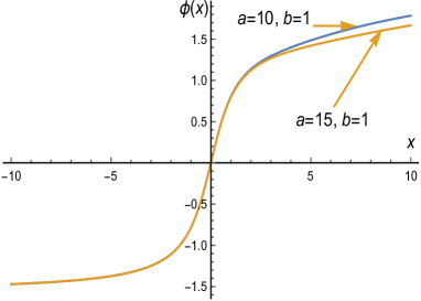
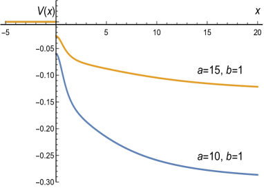
Figure 1: The scalar field $\phi(x)$ (left) and the potential $V(x)$ (right) in Example 2

On the other hand, the throat radius (26) depends on the same constants $n$ and ${\overline{k}}$ and will not be too large if they take modest values. Thus, for $n/{\overline{k}}=14$, Eq. (26) gives $r_{\min}\approx 76{\overline{k}}p_{-}$. To obtain a large enough throat for passing of a macroscopic body, say, $r_{\min}=10$ meters, one has to suppose ${\overline{k}}\sim 10^{18}$.

4.2 Example 2: ST asymptotically AdS wormholes

With nonzero potentials $V(\phi)$, in most cases solutions can be found only numerically, with one exception: the case $K=0$ in Eq. (17). It then follows $P=cA$, $c={\rm const}$, and Eq. (13) takes the form

$$[A^{3}(R/A)^{\prime}]^{\prime}=2A.$$ (27)

It is a single equation for two functions $A(x)$ and $R(x)$. It can be solved by quadratures if one specifies $A(x)$: indeed, Eq. (27) can be rewritten as

$$\Big{(}\frac{R}{A}\Big{)}^{\prime}=\frac{2}{A^{3}}\int A(x)dx.$$ (28)

We here want to obtain an example with an asymptotically flat 4D space-time on the left end and an AdS asymptotic on the right, which corresponds to $A\to 1$ as $x\to-\infty$ and $A\sim x^{2}$ as $x\to+\infty$. It is, however, hard to find $A(x)$ with the above properties that would lead to good analytic expressions of other quantities. We therefore consider an example with the following piecewise smooth function $A(x)$:

$${}A(x)=\left\{\begin{array}[]{ll}1,&x\leq 0,\\ 1+3x^{2}/a^{2},&x\geq 0,\end{array}\right.$$ (31)

with $a={\rm const}>0$. Then we must further solve the equations separately for $x<0$ and $x>0$ and match the solutions at $x=0$. At $x<0$ Eq. (27) leads to $R^{\prime\prime}=2$, hence we can take

$$R(x)\equiv r^{2}(x)=x^{2}+b^{2}\quad\ (x\leq 0),$$ (32)

with $b={\rm const}>0$ (evidently, this means that $x=0$ will be a throat of radius $b$). Further on, from (11) and (12) we find without loss of generality

$$V(x)\equiv 0,\ \ \ \phi(x)=\arctan(x/b)\ \ \ (x\leq 0).$$ (33)

The same functions at $x>0$ are also easily calculated: from (28) it follows

$$R(x)=\Big{(}1+\frac{3x^{2}}{a^{2}}\Big{)}\biggl{[}b^{2}+\frac{x^{2}(1+2x^{2}/a^{2})}{(1+3x^{2}/a^{2})^{2}}\biggr{]},$$ (34)

where the emerging integration constant is chosen to provide continuity at $x=0$. The potential $V(x)$ is then found from (11) (recall that $P(x)=cA(x)$):

$${}V(x)=-\frac{30}{a^{2}}$$

$${}+\frac{12[b^{2}x^{2}+a^{2}(2b^{2}+x^{2})]}{9b^{2}x^{4}+a^{4}(b^{2}+x^{2})+2a^{2}x^{2}(3b^{2}+x^{2})}.$$ (35)

At large $x$ ($x\to\infty$), we have

$${}R(x)=\Big{(}\frac{2}{3}+\frac{3b^{2}}{a^{2}}\Big{)}x^{2}+O(1),\quad P(x)=\frac{3cx^{2}}{a^{2}}+c,$$

$${}V(x)=-\frac{30}{a^{2}}+\frac{12(a^{2}+b^{2})}{(2a^{2}+9b^{2})x^{2}}+o(x^{-2}).$$ (36)

Thus the solution has a 6D AdS asymptotic behavior (with the curvature radius $a/\sqrt{3}$), corresponding to a negative constant $V$ which here plays the role of a cosmological constant. As already mentioned, the potential $V$ is zero at negative $x$ and has a jump at $x=0$ due to a jump in $A^{\prime\prime}$. The expression for $\phi(x)$ is found from (12) numerically, see the figure; this function is made continuous at $x=0$ by choosing the integration constants, but the derivative $\phi^{\prime}$ suffers a jump (though it is not evident in the plot). The monotonic nature of $\phi(x)$ makes the potential $V(\phi)$ well defined. The jumps in both $V(x)$ and $\phi^{\prime}(x)$ at $x=0$ could be easily removed by choosing $A(x)$ smoother than $\rm C^{1}$ at $x=0$, which is possible by making a suitable arbitrarily small addition to (31).

5 Concluding remarks

The results can be summarized as follows. We have considered static solutions with the metric (3) in 6D GR with a minimally coupled scalar field as a source of gravity and selected the kinds of asymptotic behavior of the metric functions compatible with the field equations. It has turned out that the choice of possible behaviors is rather narrow, and in particular, Rubin wormholes (as described in the introduction) are impossible in this framework. Instead, we have found another type of wormhole which lead from our universe with small extra dimensions to a universe with large extra dimensions where space-time is effectively 6-dimensional and should possess quite unusual physics. In our explicit examples of such configurations the extra dimensions have the geometry of a 2-torus. The first example represents a special case of a well-known general solution with a massless scalar field [20, 21], where the extra factor space has a large constant size at the “far end”; in the other example, with a nonzero potential $V(\phi)$, the “far end” has a 6D AdS geometry.

The existence of such configurations or their analogs with a different number of extra dimensions in our universe cannot be a priori excluded, and their possible astrophysical consequences could be a subject of further studies.

It should be noted that the analysis performed in Section 3 certainly did not cover all opportunities: we only considered asymptotically flat and AdS behaviors of the metric, whereas other, more complicated cases are also possible. For instance, of particular interest is a de Sitter asymptotic which will lead to space-times with horizons and very probably to new cosmological models of “black universe” type, where the cosmological expansion starts from a Killing horizon instead of a singularity, see, e.g. [1, 24, 25, 26] and references therein.

One more subject of a future study can be a relationship between the present scalar-vacuum system and multidimensional gravity with curvature-nonlinear actions [1, 5] in different conformal frames in application to space-times of the type considered here and in [5].

5.1 Acknowledgments

We thank Sergei Rubin and Sergei Bolokhov for numerous helpful discussions. The work of KB was partly performed within the framework of the Center FRPP supported by MEPhI Academic Excellence Project (contract No. 02.a03.21.0005, 27.08.2013). This work was also funded by the Ministry of Education and Science of the Russian Federation on the program to improve the competitiveness of the RUDN University among the world leading research and education centers in 2016–2020 and by RFBR grant 16-02-00602..

References

- [1] K. A. Bronnikov and S. G. Rubin, Black Holes, Cosmology, and Extra Dimensions (World Scientific, 2012).
- [2] V. N. Melnikov, Grav. Cosmol. 22, 80–96 (2016).
- [3] V. D. Ivashchuk and V. N. Melnikov, Grav. Cosmol. 22, 166–178 (2016).
- [4] T. Clifton, P. G. Ferreira, A. Padilla, and C. Skordis, “Modified gravity and cosmology”, Phys. Rep. 513, 1–189 (2012), arXiv: 1106.2476.
- [5] S. G. Rubin, “Interpenetrating subspaces as a funnel to extra space,” Phys. Lett. B 759, 622 (2016); arXiv: 1603.03880.
- [6] M. Visser, Lorentzian Wormholes: from Einstein to Hawking (AIP, Woodbury, 1995).
- [7] F. S. N. Lobo, “Exotic solutions in general relativity:traversable wormholes and warp drive” spacetimes,” in Classical and Quantum Gravity Research (Nova Sci. Pub., 2008), p. 1–78; arXiv: 0710.4474.
- [8] V. Dzhunushaliev, V. Folomeev, and A. Urazalina, Int. J. Mod. Phys. D 24, 1550097 (2015); arXiv: 1506.03897.
- [9] K. A. Bronnikov and A. M. Galiakhmetov, Grav. Cosmol. 21, 283 (2015); arXiv: 1508.01114.
- [10] R. Myrzakulov, L. Sebastiani, S. Vagnozzi, and S. Zerbini, Class. Quantum Grav. 33 (12), 125005 (2016); arXiv: 1510.02284.
- [11] R. Aurich, S. Lustig, F. Steiner, and H. Then, Class. Quantum Grav. 21, 4901 (2004); astro-ph/0403597.
- [12] Frank Steiner, “Do black holes exist in a finite universe having the topology of a flat 3-torus?”, arXiv: 1608.03133.
- [13] D. Hochberg and M. Visser, Phys. Rev. D 56, 4745 (1997); gr-qc/9704082.
- [14] K. A. Bronnikov and A. A. Starobinsky, Pis’ma v ZhETF 85, 3–8 (2007); JETP Lett. 85 1–5 (2007); gr-qc/0612032.
- [15] K. A. Bronnikov, M. V. Skvortsova, and A. A. Starobinsky, Grav. Cosmol. 16, 216–222 (2010); ArXiv: 1005.3262.
- [16] K. A. Bronnikov and Sung-Won Kim, Phys. Rev. D 67, 064027 (2003); gr-qc/0212112.
- [17] G. Dotti, J. Oliva, and R. Troncoso, Phys. Rev. D 76, 064038 (2007); arXiv: 0706.1830.
- [18] T. Harko, F. S. N. Lobo, M. K. Mak, and S. V. Sushkov, Phys. Rev. D 87, 067504 (2013); arXiv: 1301.6878.
- [19] K. A. Bronnikov, J. C. Fabris and S. V. B. Gonçalves, J. Phys. A: Math. Theor. 40, 6835–6840 (2007).
- [20] K. A. Bronnikov, Grav. Cosmol. 1, 67 (1995); gr-qc/9505020.
- [21] K. A. Bronnikov, V. D. Ivashchuk, and V. N. Melnikov, Grav. Cosmol. 3, 205 (1997); gr-qc/9710054.
- [22] K. A. Bronnikov, Acta Phys. Pol. B 4, 251 (1973).
- [23] H. G. Ellis, J. Math. Phys. 14, 104 (1973).
- [24] K. A. Bronnikov and J. C. Fabris, Phys. Rev. Lett. 96, 251101 (2006); gr-qc/0511109.
- [25] K. A. Bronnikov, V. N. Melnikov, and H. Dehnen, Gen. Rel. Grav. 39, 973 (2007); gr-qc/0611022.
- [26] S. V. Bolokhov, K. A. Bronnikov, and M. V. Skvortsova, Class. Quantum Grav. 29, 245006 (2012); arXiv: 1208.4619.