Real space electrostatics for multipoles. III. Dielectric Properties

Abstract

In the first two papers in this series, we developed new shifted potential (SP), gradient shifted force (GSF), and Taylor shifted force (TSF) real-space methods for multipole interactions in condensed phase simulations. Here, we discuss the dielectric properties of fluids that emerge from simulations using these methods. Most electrostatic methods (including the Ewald sum) require correction to the conducting boundary fluctuation formula for the static dielectric constants, and we discuss the derivation of these corrections for the new real space methods. For quadrupolar fluids, the analogous material property is the quadrupolar susceptibility. As in the dipolar case, the fluctuation formula for the quadrupolar susceptibility has corrections that depend on the electrostatic method being utilized. One of the most important effects measured by both the static dielectric and quadrupolar susceptibility is the ability to screen charges embedded in the fluid. We use potentials of mean force between solvated ions to discuss how geometric factors can lead to distance-dependent screening in both quadrupolar and dipolar fluids.

I Introduction

Over the past several years, there has been increasing interest in pairwise or “real space” methods for computing electrostatic interactions in condensed phase simulations.Wolf et al. (1999); Zahn, Schilling, and Kast (2002); Kast, Schmidt, and Schilling (2003); Beck, Armen, and Daggett (2005); Ma and Garofalini (2005); Wu and Brooks (2005); Fennell and Gezelter (2006); Fukuda (2013); Stenqvist et al. (2015); Wang, Nakamura, and Fukuda (2016) These techniques were initially developed by Wolf et al. in their work towards an $\mathcal{O}(N)$ Coulombic sum.Wolf et al. (1999) Wolf’s method of using cutoff neutralization and electrostatic damping is able to obtain excellent agreement with Madelung energies in ionic crystals.Wolf et al. (1999)

Zahn et al.Zahn, Schilling, and Kast (2002) and Fennell and Gezelter extended this method using shifted force approximations at the cutoff distance in order to conserve total energy in molecular dynamics simulations.Fennell and Gezelter (2006) Other recent advances in real-space methods for systems of point charges have included explicit elimination of the net multipole moments inside the cutoff sphere around each charge site.Fukuda (2013); Wang, Nakamura, and Fukuda (2016)

In the previous two papers in this series, we developed three generalized real space methods: shifted potential (SP), gradient shifted force (GSF), and Taylor shifted force (TSF).Lamichhane, Gezelter, and Newman (2014); Lamichhane, Newman, and Gezelter (2014) These methods evaluate electrostatic interactions for charges and higher order multipoles using a finite-radius cutoff sphere. The neutralization and damping of local moments within the cutoff sphere is a multipolar generalization of Wolf’s sum. In the GSF and TSF methods, additional terms are added to the potential energy so that forces and torques also vanish smoothly at the cutoff radius. This ensures that the total energy is conserved in molecular dynamics simulations.

One of the most stringent tests of any new electrostatic method is the fidelity with which that method can reproduce the bulk-phase polarizability or equivalently, the dielectric properties of a fluid. Before the advent of computer simulations, Kirkwood and Onsager developed fluctuation formulae for the dielectric properties of dipolar fluids.Kirkwood (1939); Onsager (1936) Along with projections of the frequency-dependent dielectric to zero frequency, these fluctuation formulae are now widely used to predict the static dielectric constants of simulated materials.

If we consider a system of dipolar or quadrupolar molecules under the influence of an external field or field gradient, the net polarization of the system will largely be proportional to the applied perturbation.Chitanvis (1996); Stern and Feller (2003); Slavchov and Ivanov (2014); Slavchov (2014) In simulations, the net polarization of the system is also determined by the interactions between the molecules. Therefore the macroscopic polarizability obtained from a simulation depends on the details of the electrostatic interaction methods that were employed in the simulation. To determine the relevant physical properties of the multipolar fluid from the system fluctuations, the interactions between molecules must be incorporated into the formalism for the bulk properties.

In most simulations, bulk materials are treated using periodic replicas of small regions, and this level of approximation requires corrections to the fluctuation formulae that were derived for the bulk fluids. In 1983 Neumann proposed a general formula for evaluating dielectric properties of dipolar fluids using both Ewald and real-space cutoff methods.Neumann (1983) Steinhauser and Neumann used this formula to evaluate the corrected dielectric constant for the Stockmayer fluid using two different methods: Ewald-Kornfeld (EK) and reaction field (RF) methods.Neumann and Steinhauser (1983)

Zahn et al.Zahn, Schilling, and Kast (2002) utilized this approach and evaluated the correction factor for using damped shifted charge-charge kernel. This was later generalized by Izvekov et al.,Izvekov, Swanson, and Voth (2008) who noted that the expression for the dielectric constant reduces to widely-used conducting boundary formula for real-space methods that have first derivatives that vanish at the cutoff radius.

One of the primary topics of this paper is the derivation of correction factors for the three new real space methods. The corrections are modifications to fluctuation expressions to account for truncation, shifting, and damping of the field and field gradient contributions from other multipoles. We find that the correction formulae for dipolar molecules depends not only on the methodology being used, but also on whether the molecular dipoles are treated using point charges or point dipoles. We derive correction factors for both cases.

In quadrupolar fluids, the relationship between quadrupolar susceptibility and dielectric screening is not as straightforward as in the dipolar case. The effective dielectric constant depends on the geometry of the external (or internal) field perturbation.Ernst et al. (1992) Significant efforts have been made to increase our understanding the dielectric properties of these fluids,Jeon and Kim (2003a, b); Chitanvis (1996) although a general correction formula has not yet been developed.

In this paper we derive general formulae for calculating the quadrupolar susceptibility of quadrupolar fluids. We also evaluate the correction factor for SP, GSF, and TSF methods for quadrupolar fluids interacting via point charges, point dipoles or directly through quadrupole-quadrupole interactions.

We also calculate the screening behavior for two ions immersed in multipolar fluids to estimate the distance dependence of charge screening in both dipolar and quadrupolar fluids. We use three distinct methods to compare our analytical results with computer simulations (see Fig. 1):

1. responses of the fluid to external perturbations,

2. fluctuations of system multipole moments, and

3. potentials of mean force between solvated ions,

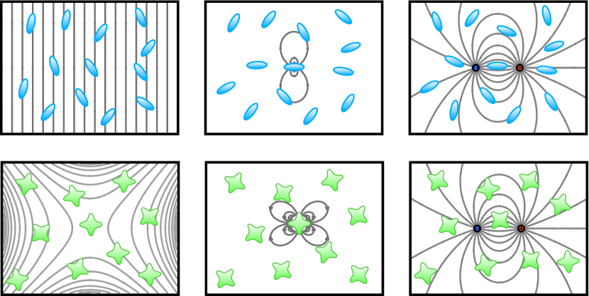
Figure 1: Dielectric properties of a fluid measure the response to external electric fields and gradients (left), or internal fields and gradients generated by the molecules themselves (center), or fields produced by embedded ions (right). The dielectric constant ($\epsilon$) measures all three responses in dipolar fluids (top). In quadrupolar liquids (bottom), the relevant bulk property is the quadrupolar susceptibility ($\chi_{Q}$), and the geometry of the field determines the effective dielectric screening.

Under the influence of weak external fields, the bulk polarization of the system is primarily a linear response to the perturbation, where the proportionality constant depends on the electrostatic interactions between the multipoles. The fluctuation formulae connect bulk properties of the fluid to equilibrium fluctuations in the system multipolar moments during a simulation. These fluctuations also depend on the form of the electrostatic interactions between molecules. Therefore, the connections between the actual bulk properties and both the computed fluctuation and external field responses must be modified accordingly.

The potential of mean force (PMF) allows calculation of an effective dielectric constant or screening factor from the potential energy between ions before and after dielectric material is introduced. Computing the PMF between embedded point charges is an additional check on the bulk properties computed via the other two methods.

II The Real-Space Methods

In the first paper in this series, we derived interaction energies, as well as expressions for the forces and torques for point multipoles interacting via three new real-space methods.Lamichhane, Gezelter, and Newman (2014) The Taylor shifted-force (TSF) method modifies the electrostatic kernel, $f(r)=1/r$, so that all forces and torques go smoothly to zero at the cutoff radius,

$$U^{\text{TSF}}_{ab}=M_{a}M_{b}f_{n}(r).$$ (1)

Here the multipole operator for site $a$, $M_{a}$, is expressed in terms of the point charge, $C_{a}$, dipole, ${\bf D}_{a}$, and quadrupole, $\mathsf{Q}_{a}$, for object $a$, etc. Because each of the multipole operators includes gradient operators (one for a dipole, two for a quadrupole, etc.), an approximate electrostatic kernel, $f_{n}(r)$ is Taylor-expanded around the cutoff radius, so that $n+1$ derivatives vanish as $r\rightarrow r_{c}$. This ensures smooth convergence of the energy, forces, and torques as molecules leave and reenter each others cutoff spheres. The order of the Taylor expansion is determined by the multipolar order of the interaction. That is, smooth quadrupole-quadrupole forces require the fifth derivative to vanish at the cutoff radius, so the appropriate function Taylor expansion will be of fifth order.

Following this procedure results in separate radial functions for each of the distinct orientational contributions to the potential. For example, in dipole-dipole interactions, the direct dipole dot product ($\mathbf{D}_{a}\cdot\mathbf{D}_{b}$) is treated differently than the dipole-distance dot products:

$$U_{\mathbf{D}_{a}\mathbf{D}_{b}}(r)=-\frac{1}{4\pi\epsilon_{0}}\left[\left(\mathbf{D}_{a}\cdot\mathbf{D}_{b}\right)v_{21}(r)+\left(\mathbf{D}_{a}\cdot\hat{\mathbf{r}}\right)\left(\mathbf{D}_{b}\cdot\hat{\mathbf{r}}\right)v_{22}(r)\right]$$ (2)

In standard electrostatics, the two radial functions, $v_{21}(r)$ and $v_{22}(r)$, are proportional to $1/r^{3}$, but they have distinct radial dependence in the TSF method. Careful choice of these functions makes the forces and torques vanish smoothly as the molecules drift beyond the cutoff radius (even when those molecules are in different orientations).

A second and somewhat simpler approach involves shifting the gradient of the Coulomb potential for each particular multipole order,

$$U^{\text{GSF}}_{ab}=\sum\left[U(\mathbf{r},\mathsf{A},\mathsf{B})-U(r_{c}\hat{\mathbf{r}},\mathsf{A},\mathsf{B})-(r-r_{c})\hat{\mathbf{r}}\cdot\nabla U(r_{c}\hat{\mathbf{r}},\mathsf{A},\mathsf{B})\right]$$ (3)

where the sum describes a separate force-shifting that is applied to each orientational contribution to the energy, i.e. $v_{21}$ and $v_{22}$ are shifted separately. In this expression, $\hat{\mathbf{r}}$ is the unit vector connecting the two multipoles ($a$ and $b$) in space, and $\mathsf{A}$ and $\mathsf{B}$ represent the orientations of the multipoles. Because this procedure is equivalent to using the gradient of an image multipole placed at the cutoff sphere for shifting the force, this method is called the gradient shifted-force (GSF) approach.

Both the TSF and GSF approaches can be thought of as multipolar extensions of the original damped shifted-force (DSF) approach that was developed for point charges. There is also a multipolar extension of the Wolf sum that is obtained by projecting an image multipole onto the surface of the cutoff sphere, and including the interactions with the central multipole and the image. This effectively shifts only the total potential to zero at the cutoff radius,

$$U^{\text{SP}}_{ab}=\sum\left[U(\mathbf{r},\mathsf{A},\mathsf{B})-U(r_{c}\hat{\mathbf{r}},\mathsf{A},\mathsf{B})\right]$$ (4)

where the sum again describes separate potential shifting that is done for each orientational contribution to the energy. The potential energy between a central multipole and other multipolar sites goes smoothly to zero as $r\rightarrow r_{c}$, but the forces and torques obtained from this shifted potential (SP) approach are discontinuous at $r_{c}$.

All three of the new real space methods share a common structure: the various orientational contributions to multipolar interaction energies require separate treatment of their radial functions, and these are tabulated for both the raw Coulombic kernel ($1/r$) as well as the damped kernel ($\mathrm{erfc}(\alpha r)/r$), in the first paper of this series.Lamichhane, Gezelter, and Newman (2014) The second paper in this series evaluated the fidelity with which the three new methods reproduced Ewald-based results for a number of model systems.Lamichhane, Newman, and Gezelter (2014) One of the major findings was that moderately-damped GSF simulations produced nearly identical behavior with Ewald-based simulations, but the real-space methods scale linearly with system size.

III Dipolar Fluids and the Dielectric Constant

Dielectric properties of a fluid arise mainly from responses of the fluid to either applied fields or transient fields internal to the fluid. In response to an applied field, the molecules have electronic polarizabilities, changes to internal bond lengths and angles, and reorientations towards the direction of the applied field. There is an added complication that in the presence of external field, the perturbation experienced by any single molecule is not only due to the external field but also to the fields produced by the all other molecules in the system.

III.1 Response to External Perturbations

In the presence of uniform electric field $\mathbf{E}$, an individual molecule with a permanent dipole moment $p_{o}$ will realign along the direction of the field with an average polarization given by

$$\braket{\mathbf{p}}=\epsilon_{0}\alpha_{p}\mathbf{E},$$ (5)

where $\alpha_{p}={p_{o}}^{2}/3\epsilon_{0}k_{B}T$ is the contribution to molecular polarizability due solely to reorientation dynamics. Because the applied field must overcome thermal motion, the orientational polarization depends inversely on the temperature.

A condensed phase system of permanent dipoles will also polarize along the direction of an applied field. The polarization density of the system is

$$\textbf{P}=\epsilon_{o}\chi_{D}\mathbf{E},$$ (6)

where the constant $\chi_{D}$ is the dipole susceptibility, which is an emergent property of the dipolar fluid, and is the quantity most directly related to the static dielectric constant, $\epsilon=1+\chi_{D}$.

III.2 Fluctuation Formula

For a system of dipolar molecules at thermal equilibrium, we can define both a system dipole moment, $\mathbf{M}=\sum_{i}\mathbf{p}_{i}$ as well as a dipole polarization density, $\mathbf{P}=\braket{\mathbf{M}}/V$. The polarization density can be expressed approximately in terms of fluctuations in the net dipole moment,

$$\mathbf{P}=\epsilon_{o}\frac{\braket{\mathbf{M}^{2}}-{\braket{\mathbf{M}}}^{2}}{3\epsilon_{o}Vk_{B}T}\bf{E}$$ (7)

This has structural similarity with the Boltzmann average for the polarization of a single molecule. Here $\braket{\mathbf{M}^{2}}-{\braket{\mathbf{M}}}^{2}$ measures fluctuations in the net dipole moment,

$$\langle\mathbf{M}^{2}\rangle-\langle\mathbf{M}\rangle^{2}=\langle M_{x}^{2}+M_{y}^{2}+M_{z}^{2}\rangle-\left(\langle M_{x}\rangle^{2}+\langle M_{y}\rangle^{2}+\langle M_{z}\rangle^{2}\right).$$ (8)

When no applied electric field is present, the ensemble average of both the net dipole moment $\braket{\mathbf{M}}$ and dipolar polarization $\bf{P}$ tends to vanish but $\braket{\mathbf{M}^{2}}$ does not. The bulk dipole polarizability can therefore be written

$$\alpha_{D}=\frac{\braket{\mathbf{M}^{2}}-{\braket{\mathbf{M}}}^{2}}{3\epsilon_{o}Vk_{B}T}.$$ (9)

The susceptibility ($\chi_{D}$) and bulk polarizability ($\alpha_{D}$) both measure responses of a dipolar system. However, $\chi_{D}$ is the bulk property assuming an infinite system and exact treatment of electrostatic interactions, while $\alpha_{D}$ is relatively simple to compute from numerical simulations. One of the primary aims of this paper is to provide the connection between the bulk properties ($\epsilon,\chi_{D}$) and the computed quantities ($\alpha_{D}$) that have been adapted for the new real-space methods.

III.3 Correction Factors

In the presence of a uniform external field $\mathbf{E}^{\circ}$, the total electric field at $\mathbf{r}$ depends on the polarization density at all other points in the system,Neumann (1983)

$$\mathbf{E}(\mathbf{r})=\mathbf{E}^{\circ}(\mathbf{r})+\frac{1}{4\pi\epsilon_{o}}\int d\mathbf{r}^{\prime}\mathbf{T}(\mathbf{r}-\mathbf{r}^{\prime})\cdot{\mathbf{P}(\mathbf{r}^{\prime})}.$$ (10)

$\mathbf{T}$ is the dipole interaction tensor connecting dipoles at $\mathbf{r}^{\prime}$ with the point of interest ($\mathbf{r}$), where the integral is done over all space. Because simulations utilize periodic boundary conditions or spherical cutoffs, the integral is normally carried out either over the domain ($0<r<r_{c}$) or in reciprocal space.

In simulations of dipolar fluids, the molecular dipoles may be represented either by closely-spaced point charges or by point dipoles (see Fig. 2).

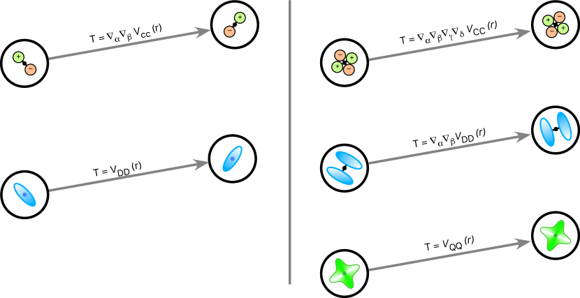
Figure 2: In the real-space electrostatic methods, the molecular dipole tensor, $\mathbf{T}_{\alpha\beta}(r)$, is not the same for charge-charge interactions as for point dipoles (left panel). The same holds true for the molecular quadrupole tensor (right panel), $\mathbf{T}_{\alpha\beta\gamma\delta}(r)$, which can have distinct forms if the molecule is represented by charges, dipoles, or point quadrupoles.

In the case where point charges are interacting via an electrostatic kernel, $v(r)$, the effective molecular dipole tensor, $\mathbf{T}$ is obtained from two successive applications of the gradient operator to the electrostatic kernel,

$$T_{\alpha\beta}(\mathbf{r}) = \nabla_{\alpha}\nabla_{\beta}\left(v(r)\right)$$ (11)

$$= \delta_{\alpha\beta}\left(\frac{1}{r}v^{\prime}(r)\right)+\frac{r_{\alpha}r_{\beta}}{r^{2}}\left(v^{\prime\prime}(r)-\frac{1}{r}v^{\prime}(r)\right)$$ (12)

where $v(r)$ may be either the bare kernel ($1/r$) or one of the modified (Wolf or DSF) kernels. This tensor describes the effective interaction between molecular dipoles ($\mathbf{D}$) in Gaussian units as $-\mathbf{D}\cdot\mathbf{T}\cdot\mathbf{D}$.

When utilizing any of the three new real-space methods for point dipoles, the tensor is explicitly constructed,

$$T_{\alpha\beta}(\mathbf{r})=\delta_{\alpha\beta}v_{21}(r)+\frac{r_{\alpha}r_{\beta}}{r^{2}}v_{22}(r)$$ (13)

where the functions $v_{21}(r)$ and $v_{22}(r)$ depend on the level of the approximation.Lamichhane, Gezelter, and Newman (2014); Lamichhane, Newman, and Gezelter (2014) Although the Taylor-shifted (TSF) and gradient-shifted (GSF) models produce to the same $v(r)$ function for point charges, they have distinct forms for the dipole-dipole interaction.

Using the constitutive relation in Eq. (6), the polarization density $\mathbf{P}(\mathbf{r})$ is given by,

$$\mathbf{P}(\mathbf{r})=\epsilon_{o}\chi_{D}\left(\mathbf{E}^{\circ}(\mathbf{r})+\frac{1}{4\pi\epsilon_{o}}\int d\mathbf{r}^{\prime}\mathbf{T}(\mathbf{r}-\mathbf{r}^{\prime})\cdot\mathbf{P}(\mathbf{r}^{\prime})\right).$$ (14)

Note that $\chi_{D}$ depends explicitly on the details of the dipole interaction tensor. Neumann et al. Neumann (1983); Neumann and Steinhauser (1983); Neumann, Steinhauser, and Pawley (1984); Neumann (1985) derived an elegant way to modify the fluctuation formula to correct for approximate interaction tensors. This correction was derived using a Fourier representation of the interaction tensor, $\tilde{\mathbf{T}}(\mathbf{k})$, and involves the quantity,

$$\mathsf{A}=\frac{3}{4\pi}\tilde{\mathbf{T}}(0)=\frac{3}{4\pi}\int_{V}d\mathbf{r}\mathbf{T}(\mathbf{r})$$ (15)

which is the $k\rightarrow 0$ limit of $\tilde{\mathbf{T}}(\mathbf{k})$. Note that the integration of the dipole tensors, Eqs. (12) and (13), over spherical volumes yields values only along the diagonal. Additionally, the spherical symmetry of $\mathbf{T}(\mathbf{r})$ insures that all diagonal elements are identical. For this reason, $\mathsf{A}$ can be written as a scalar constant ($A$) multiplying the unit tensor.

Using the quantity $A$ (originally called $Q$ in refs. Neumann, 1983; Neumann and Steinhauser, 1983; Neumann, Steinhauser, and Pawley, 1984; Neumann, 1985), the dielectric constant can be computed

$$\epsilon=\frac{3+(A+2)(\epsilon_{CB}-1)}{3+(A-1)(\epsilon_{CB}-1)}$$ (16)

where $\epsilon_{CB}$ is the widely-used conducting boundary expression for the dielectric constant,

$$\epsilon_{CB}=1+\frac{\braket{\bf{M}^{2}}-{\braket{\bf{M}}}^{2}}{3\epsilon_{o}Vk_{B}T}=1+\alpha_{D}.$$ (17)

Eqs. (16) and (17) allow estimation of the static dielectric constant from fluctuations computed directly from simulations, with the understanding that Eq. (16) is extraordinarily sensitive when $A$ is far from unity.

We have utilized the Neumann et al. approach for the three new real-space methods, and obtain method-dependent correction factors. The expression for the correction factor also depends on whether the simulation involves point charges or point dipoles to represent the molecular dipoles. These corrections factors are listed in Table 1. We note that the GSF correction factor for point dipoles has been independently derived by Stenqvist et al.Stenqvist et al. (2015)

Table 1: Expressions for the dipolar correction factor ($A$) for the real-space electrostatic methods in terms of the damping parameter ($\alpha$) and the cutoff radius ($r_{c}$). The Ewald-Kornfeld result derived in Refs. Adams, 1980; Adams and Adams, 1981; Neumann, 1983 is shown for comparison using the Ewald convergence parameter ($\kappa$) and the real-space cutoff value ($r_{c}$).

	Molecular Representation
Method	point charges	point dipoles
Shifted Potential (SP)	$\mathrm{erf}(r_{c}\alpha)-\frac{2\alpha r_{c}}{\sqrt{\pi}}e^{-\alpha^{2}r_{c}^{2}}$	$\mathrm{erf}(r_{c}\alpha)-\frac{2\alpha r_{c}}{\sqrt{\pi}}\left(1+\frac{2\alpha^{2}{r_{c}}^{2}}{3}\right)e^{-\alpha^{2}{r_{c}}^{2}}$
Gradient-shifted (GSF)	1	$\mathrm{erf}(\alpha r_{c})-\frac{2\alpha r_{c}}{\sqrt{\pi}}\left(1+\frac{2\alpha^{2}r_{c}^{2}}{3}+\frac{\alpha^{4}r_{c}^{4}}{3}\right)e^{-\alpha^{2}r_{c}^{2}}$
Taylor-shifted (TSF)	1
Ewald-Kornfeld (EK)	$\mathrm{erf}(r_{c}\kappa)-\frac{2\kappa r_{c}}{\sqrt{\pi}}e^{-\kappa^{2}r_{c}^{2}}$

Note that for point charges, the GSF and TSF methods produce estimates of the dielectric that need no correction, and the TSF method likewise needs no correction for point dipoles.

IV Quadrupolar Fluids and the Quadrupolar Susceptibility

IV.1 Response to External Perturbations

A molecule with a permanent quadrupole, $\mathsf{q}$, will align in the presence of an electric field gradient $\nabla\mathbf{E}$. The anisotropic polarization of the quadrupole is given by,Adu-Gyamfi (1978, 1981)

$$\braket{\mathsf{q}}-\frac{\mathbf{I}}{3}\mathrm{Tr}(\mathsf{q})=\epsilon_{o}\alpha_{q}\nabla\mathbf{E},$$ (18)

where $\alpha_{q}=q_{o}^{2}/15\epsilon_{o}k_{B}T$ is a molecular quadrupole polarizability and $q_{o}$ is an effective quadrupole moment for the molecule,

$$q_{o}^{2}=3\mathsf{q}:\mathsf{q}-\mathrm{Tr}(\mathsf{q})^{2}.$$ (19)

Note that quadrupole calculations involve tensor contractions (double dot products) between rank two tensors, which are defined as

$$\mathsf{A}\colon\mathsf{B}=\sum_{\alpha}\sum_{\beta}A_{\alpha\beta}B_{\beta\alpha}.$$ (20)

In the presence of an external field gradient, a system of quadrupolar molecules also organizes with an anisotropic polarization,

$$\mathsf{Q}-\frac{\mathbf{I}}{3}\mathrm{Tr}(\mathsf{Q})=\epsilon_{o}\chi_{Q}\nabla\mathbf{E}$$ (21)

where $\mathsf{Q}$ is the traced quadrupole density of the system and $\chi_{Q}$ is a macroscopic quadrupole susceptibility which has dimensions of $\mathrm{length}^{-2}$. Equivalently, the traceless form may be used,

$$\mathsf{\Theta}=3\epsilon_{o}\chi_{Q}\nabla\mathbf{E},$$ (22)

where $\mathsf{\Theta}=3\mathsf{Q}-\mathbf{I}\mathrm{Tr}(\mathsf{Q})$ is the traceless tensor that also describes the system quadrupole density. It is this tensor that will be utilized to derive correction factors below.

IV.2 Fluctuation Formula

As in the dipolar case, we may define a system quadrupole moment, $\mathsf{M}_{Q}=\sum_{i}\mathsf{q}_{i}$ and the traced quadrupolar density, $\mathsf{Q}=\mathsf{M}_{Q}/V$. A fluctuation formula can be written for a system comprising quadrupolar molecules,Logan (1981, 1982a, 1982b)

$$\mathsf{Q}-\frac{\mathbf{I}}{3}\mathrm{Tr}(\mathsf{Q})=\epsilon_{o}\frac{\braket{\mathsf{M}_{Q}^{2}}-{\braket{\mathsf{M}_{Q}}}^{2}}{15\epsilon_{o}Vk_{B}T}\nabla\mathbf{E}.$$ (23)

Some care is needed in the definitions of the averaged quantities. These refer to the effective quadrupole moment of the system, and they are computed as follows,

$$\braket{\mathsf{M}_{Q}^{2}} =\braket{3\mathsf{M}_{Q}:\mathsf{M}_{Q}-\mathrm{Tr}(\mathsf{M}_{Q})^{2}}$$ (24)

$$\braket{\mathsf{M}_{Q}}^{2} =3\braket{\mathsf{M}_{Q}}:\braket{\mathsf{M}_{Q}}-\mathrm{Tr}(\braket{\mathsf{M}_{Q}})^{2}$$ (25)

The bulk quadrupolarizability is given by,

$$\alpha_{Q}=\frac{\braket{\mathsf{M}_{Q}^{2}}-{\braket{\mathsf{M}_{Q}}}^{2}}{15\epsilon_{o}Vk_{B}T}.$$ (26)

Note that as in the dipolar case, $\alpha_{Q}$ and $\chi_{Q}$ are distinct quantities. $\chi_{Q}$ measures the bulk response assuming an infinite system and exact electrostatics, while $\alpha_{Q}$ is relatively simple to compute from numerical simulations. As in the dipolar case, estimation of the true bulk property requires correction for truncation, shifting, and damping of the electrostatic interactions.

IV.3 Correction Factors

In this section we generalize the treatment of Neumann et al. for quadrupolar fluids. Interactions involving multiple quadrupoles are rank 4 tensors, and we therefore describe quantities in this section using Einstein notation.

In the presence of a uniform external field gradient, $\partial_{\alpha}{E}^{\circ}_{\beta}$, the total field gradient at $\mathbf{r}$ depends on the quadrupole polarization density at all other points in the system,

$$\partial_{\alpha}E_{\beta}(\mathbf{r})=\partial_{\alpha}{E}^{\circ}_{\beta}(\mathbf{r})+\frac{1}{8\pi\epsilon_{o}}\int T_{\alpha\beta\gamma\delta}({\mathbf{r}-\mathbf{r}^{\prime}})Q_{\gamma\delta}(\mathbf{r}^{\prime})d\mathbf{r}^{\prime}$$ (27)

where and $T_{\alpha\beta\gamma\delta}$ is the quadrupole interaction tensor connecting quadrupoles at $\mathbf{r}^{\prime}$ with the point of interest ($\mathbf{r}$).

In simulations of quadrupolar fluids, the molecular quadrupoles may be represented by closely-spaced point charges, by multiple point dipoles, or by a single point quadrupole (see Fig. 2). In the case where point charges are interacting via an electrostatic kernel, $v(r)$, the effective molecular quadrupole tensor can obtained from four successive applications of the gradient operator to the electrostatic kernel,

$$T_{\alpha\beta\gamma\delta}(\mathbf{r}) = \nabla_{\alpha}\nabla_{\beta}\nabla_{\gamma}\nabla_{\delta}v(r)$$ (29)

$$= \left(\delta_{\alpha\beta}\delta_{\gamma\delta}+\delta_{\alpha\gamma}\delta_{\beta\delta}+\delta_{\alpha\delta}\delta_{\beta\gamma}\right)\left(-\frac{v^{\prime}(r)}{r^{3}}+\frac{v^{\prime\prime}(r)}{r^{2}}\right)$$

$$+\left(\delta_{\alpha\beta}r_{\gamma}r_{\delta}+5\mathrm{~{}permutations}\right)\left(\frac{3v^{\prime}(r)}{r^{5}}-\frac{3v^{\prime\prime}(r)}{r^{4}}+\frac{v^{\prime\prime\prime}(r)}{r^{3}}\right)$$

$$+r_{\alpha}r_{\beta}r_{\gamma}r_{\delta}\left(-\frac{15v^{\prime}(r)}{r^{7}}+\frac{15v^{\prime\prime}(r)}{r^{6}}-\frac{6v^{\prime\prime\prime}(r)}{r^{5}}+\frac{v^{\prime\prime\prime\prime}(r)}{r^{4}}\right),$$

where $v(r)$ can either be the electrostatic kernel ($1/r$) or one of the modified (Wolf or DSF) kernels.

Similarly, when representing quadrupolar molecules with multiple point dipoles, the molecular quadrupole interaction tensor can be obtained using two successive applications of the gradient operator to the dipole interaction tensor,

$$T_{\alpha\beta\gamma\delta}(\mathbf{r}) = \nabla_{\alpha}\nabla_{\beta}T_{\gamma\delta}(\mathbf{r})$$ (31)

$$= \delta_{\alpha\beta}\delta_{\gamma\delta}\frac{v^{\prime}_{21}(r)}{r}+\left(\delta_{\alpha\gamma}\delta_{\beta\delta}+\delta_{\alpha\delta}\delta_{\beta\gamma}\right)\frac{v_{22}(r)}{r^{2}}$$

$$+\delta_{\gamma\delta}r_{\alpha}r_{\beta}\left(\frac{v^{\prime\prime}_{21}(r)}{r^{2}}-\frac{v^{\prime}_{21}(r)}{r^{3}}\right)$$

$$+\left(\delta_{\alpha\beta}r_{\gamma}r_{\delta}+\delta_{\alpha\gamma}r_{\beta}r_{\delta}+\delta_{\alpha\delta}r_{\gamma}r_{\beta}+\delta_{\beta\gamma}r_{\alpha}r_{\delta}+\delta_{\beta\delta}r_{\alpha}r_{\gamma}\right)\left(\frac{v^{\prime}_{22}(r)}{r^{3}}-\frac{2v_{22}(r)}{r^{4}}\right)$$

$$+r_{\alpha}r_{\beta}r_{\gamma}r_{\delta}\left(\frac{v^{\prime\prime}_{22}(r)}{r^{4}}-\frac{5v^{\prime}_{22}(r)}{r^{5}}+\frac{8v_{22}(r)}{r^{6}}\right),$$

where $T_{\gamma\delta}(\mathbf{r})$ is a dipole-dipole interaction tensor that depends on the level of the approximation (see Eq. (13)).Lamichhane, Gezelter, and Newman (2014); Lamichhane, Newman, and Gezelter (2014) Similarly $v_{21}(r)$ and $v_{22}(r)$ are the radial functions for different real space cutoff methods defined in the first paper in this series.Lamichhane, Gezelter, and Newman (2014)

For quadrupolar liquids modeled using point quadrupoles, the interaction tensor can be constructed as,

$$T_{\alpha\beta\gamma\delta}(\mathbf{r}) = \left(\delta_{\alpha\beta}\delta_{\gamma\delta}+\delta_{\alpha\gamma}\delta_{\beta\delta}+\delta_{\alpha\delta}\delta_{\beta\gamma}\right)v_{41}(r)+(\delta_{\gamma\delta}r_{\alpha}r_{\beta}+\mathrm{5\;permutations})\frac{v_{42}(r)}{r^{2}}$$ (32)

$$+r_{\alpha}r_{\beta}r_{\gamma}r_{\delta}\left(\frac{v_{43}(r)}{r^{4}}\right),$$

where again $v_{41}(r)$, $v_{42}(r)$, and $v_{43}(r)$ are radial functions defined in Paper I of the series. Lamichhane, Gezelter, and Newman (2014) Note that these radial functions have different functional forms depending on the level of approximation being employed.

The integral in Eq. (27) can be divided into two parts, $|\mathbf{r}-\mathbf{r}^{\prime}|\rightarrow 0$ and $|\mathbf{r}-\mathbf{r}^{\prime}|>0$. Since the self-contribution to the field gradient vanishes at the singularity (see the supplemental material), Eq. (27) can be written as,

$$\partial_{\alpha}E_{\beta}(\mathbf{r})=\partial_{\alpha}{E}^{\circ}_{\beta}(\mathbf{r})+\frac{1}{8\pi\epsilon_{o}}\int\limits_{|\mathbf{r}-\mathbf{r}^{\prime}|>0}T_{\alpha\beta\gamma\delta}(\mathbf{r}-\mathbf{r}^{\prime}){Q}_{\gamma\delta}(\mathbf{r}^{\prime})d\mathbf{r}^{\prime}.$$ (33)

If $\mathbf{r}=\mathbf{r}^{\prime}$ is excluded from the integration, the total gradient can be most easily expressed in terms of traceless quadrupole density as below,Logan (1981)

$$\partial_{\alpha}E_{\beta}(\mathbf{r})=\partial_{\alpha}{E}^{\circ}_{\beta}(\mathbf{r})+\frac{1}{24\pi\epsilon_{o}}\int\limits_{|\mathbf{r}-\mathbf{r}^{\prime}|>0}T_{\alpha\beta\gamma\delta}(\mathbf{r}-\mathbf{r}^{\prime})\Theta_{\gamma\delta}(\mathbf{r}^{\prime})d\mathbf{r}^{\prime},$$ (34)

where $\Theta_{\alpha\beta}=3Q_{\alpha\beta}-\delta_{\alpha\beta}Tr(Q)$ is the traceless quadrupole density. In analogy to Eq. (22) above, the quadrupole polarization density may now be related to the quadrupolar susceptibility, $\chi_{Q}$,

$$\frac{1}{3}{\Theta}_{\alpha\beta}(\mathbf{r})=\epsilon_{o}{\chi}_{Q}\left[\partial_{\alpha}{E}^{\circ}_{\beta}(\mathbf{r})+\frac{1}{24\pi\epsilon_{o}}\int\limits_{|\mathbf{r}-\mathbf{r}^{\prime}|>0}T_{\alpha\beta\gamma\delta}(\mathbf{r}-\mathbf{r}^{\prime})\Theta_{\gamma\delta}(\mathbf{r}^{\prime})d\mathbf{r}^{\prime}\right].$$ (35)

For periodic boundaries and with a uniform imposed $\partial_{\alpha}E^{\circ}_{\beta}$, the quadrupole density ${\Theta}_{\alpha\beta}$ will be uniform over the entire space. After performing a Fourier transform (see the Appendix in ref. Neumann, 1983) we obtain,

$$\frac{1}{3}\tilde{\Theta}_{\alpha\beta}(\mathbf{k})=\epsilon_{o}{\chi}_{Q}\left[{\partial_{\alpha}\tilde{E}^{\circ}_{\beta}}(\mathbf{k})+\frac{1}{24\pi\epsilon_{o}}\tilde{T}_{\alpha\beta\gamma\delta}(\mathbf{k})\tilde{\Theta}_{\gamma\delta}(\mathbf{k})\right].$$ (36)

If the applied field gradient is homogeneous over the entire volume, ${\partial_{\alpha}\tilde{E}^{\circ}_{\beta}}(\mathbf{k})=0$ except at $\mathbf{k}=0$. Similarly, the quadrupolar polarization density can also considered uniform over entire space. As in the dipolar case, Neumann (1983) the only relevant contribution from the interaction tensor will also be when $\mathbf{k}=0$. Therefore Eq. (36) can be written as,

$$\frac{1}{3}\tilde{\Theta}_{\alpha\beta}(\mathrm{0})=\epsilon_{o}{\chi}_{Q}\left[{\partial_{\alpha}\tilde{E}^{\circ}_{\beta}}(\mathrm{0})+\frac{1}{24\pi\epsilon_{o}}\tilde{T}_{\alpha\beta\gamma\delta}(\mathrm{0})\tilde{\Theta}_{\gamma\delta}(\mathrm{0})\right].$$ (37)

The quadrupolar tensor $\tilde{T}_{\alpha\beta\gamma\delta}(\mathrm{0})$ is a rank 4 tensor with 81 elements. The only non-zero elements, however, are those with two doubly-repeated indices, i.e. $\tilde{T}_{aabb}(\mathrm{0})$ and all permutations of these indices. The special case of quadruply-repeated indices, $\tilde{T}_{aaaa}(\mathrm{0})$ also survives (see appendix A). Furthermore, for the both diagonal and non-diagonal components of the quadrupolar polarization $\tilde{\Theta}_{\alpha\beta}$, we can contract the second term in Eq. 37 (see appendix A):

$$\tilde{T}_{\alpha\beta\gamma\delta}(\mathrm{0})\tilde{\Theta}_{\gamma\delta}(\mathrm{0})=8\pi\mathrm{B}\tilde{\Theta}_{\alpha\beta}(\mathrm{0}).$$ (38)

Here $\mathrm{B}=\tilde{T}_{abab}(\mathrm{0})/4\pi$ for $a\neq b$. Using this quadrupolar contraction we can solve Eq. 37 as follows

$$\frac{1}{3}\tilde{\Theta}_{\alpha\beta}(\mathrm{0}) = \epsilon_{o}{\chi}_{Q}\left[{\partial_{\alpha}\tilde{E}^{\circ}_{\beta}}(\mathrm{0})+\frac{\mathrm{B}}{3\epsilon_{o}}{\tilde{\Theta}}_{\alpha\beta}(\mathrm{0})\right]$$ (39)

$$= \left[\frac{\epsilon_{o}{\chi}_{Q}}{1-{\chi}_{Q}\mathrm{B}}\right]{\partial_{\alpha}\tilde{E}^{\circ}_{\beta}}(\mathrm{0}).$$

In real space, the correction factor is found to be,

$$\mathrm{B}=\frac{1}{4\pi}\tilde{T}_{abab}(0)=\frac{1}{4\pi}\int_{V}{T}_{abab}(\mathbf{r})d\mathbf{r},$$ (40)

which has been integrated over the interaction volume $V$ and has units of $\mathrm{length}^{-2}$.

In terms of the traced quadrupole moment, Eq. (39) can be written,

$$\mathsf{Q}-\frac{\mathbf{I}}{3}\mathrm{Tr}(\mathsf{Q})=\frac{\epsilon_{o}{\chi}_{Q}}{1-{\chi}_{Q}\mathrm{B}}\nabla\mathbf{E}^{\circ}$$ (41)

Comparing (41) and (23) we obtain,

$$\frac{\braket{\mathsf{M}_{Q}^{2}}-{\braket{\mathsf{M}_{Q}}}^{2}}{15\epsilon_{o}Vk_{B}T}=\frac{\chi_{Q}}{1-\chi_{Q}\mathrm{B}},$$ (42)

or equivalently,

$$\chi_{Q}=\frac{\braket{\mathsf{M}_{Q}^{2}}-{\braket{\mathsf{M}_{Q}}}^{2}}{15\epsilon_{o}Vk_{B}T}\left(1+\mathrm{B}\frac{\braket{\mathsf{M}_{Q}^{2}}-{\braket{\mathsf{M}_{Q}}}^{2}}{15\epsilon_{o}Vk_{B}T}\right)^{-1}.$$ (43)

Eq. (43) now expresses a bulk property (the quadrupolar susceptibility, $\chi_{Q}$) in terms of a fluctuation in the system quadrupole moment and a quadrupolar correction factor ($\mathrm{B}$). The correction factors depend on the cutoff method being employed in the simulation, and these are listed in Table 2.

In terms of the macroscopic quadrupole polarizability, $\alpha_{Q}$, which may be thought of as the “conducting boundary” version of the susceptibility,

$$\chi_{Q}=\frac{\alpha_{Q}}{1+\mathrm{B}\alpha_{Q}}.$$ (44)

If an electrostatic method produces $\mathrm{B}\rightarrow 0$, the computed quadrupole polarizability and quadrupole susceptibility converge to the same value.

Table 2: Expressions for the quadrupolar correction factor ($\mathrm{B}$) for the real-space electrostatic methods in terms of the damping parameter ($\alpha$) and the cutoff radius ($r_{c}$). The units of the correction factor are $\mathrm{length}^{-2}$ for quadrupolar fluids.

Method	Molecular Representation
	charges	dipoles	quadrupoles
Shifted Potential (SP)	$-\frac{8\alpha^{5}{r_{c}}^{3}e^{-\alpha^{2}r_{c}^{2}}}{15\sqrt{\pi}}$	$-\frac{3\mathrm{erfc(r_{c}\alpha)}}{5{r_{c}}^{2}}-\frac{2\alpha e^{-\alpha^{2}r_{c}^{2}}(9+6\alpha^{2}r_{c}^{2}+4\alpha^{4}r_{c}^{4})}{15{\sqrt{\pi}r_{c}}}$	$-\frac{16\alpha^{7}{r_{c}}^{5}e^{-\alpha^{2}r_{c}^{2}}}{45\sqrt{\pi}}$
Gradient-shifted (GSF)	$-\frac{8\alpha^{5}{r_{c}}^{3}e^{-\alpha^{2}r_{c}^{2}}}{15\sqrt{\pi}}$	0	$-\frac{4{\alpha}^{7}{r_{c}}^{5}e^{-\alpha^{2}r_{c}^{2}}(-1+2\alpha^{2}r_{c}^{2})}{45\sqrt{\pi}}$
Taylor-shifted (TSF)	$-\frac{8\alpha^{5}{r_{c}}^{3}e^{-\alpha^{2}r_{c}^{2}}}{15\sqrt{\pi}}$	$\frac{4\;\mathrm{erfc(\alpha r_{c})}}{{5r_{c}}^{2}}+\frac{8\alpha e^{-\alpha^{2}{r_{c}}^{2}}\left(3+2\alpha^{2}{r_{c}}^{2}+\alpha^{4}{r_{c}}^{4}\right)}{15\sqrt{\pi}r_{c}}$	$\frac{2\;\mathrm{erfc}(\alpha r_{c})}{{r_{c}}^{2}}+\frac{4{\alpha}e^{-\alpha^{2}r_{c}^{2}}\left(45+30\alpha^{2}{r_{c}}^{2}+12\alpha^{4}{r_{c}}^{4}+3\alpha^{6}{r_{c}}^{6}+2\alpha^{8}{r_{c}}^{8}\right)}{45\sqrt{\pi}{r_{c}}}$
Ewald-Kornfeld (EK)	$-\frac{8\kappa^{5}{r_{c}}^{3}e^{-\kappa^{2}r_{c}^{2}}}{15\sqrt{\pi}}$

V Screening of Charges by Multipolar Fluids

In a dipolar fluid, the static dielectric constant is also a measure of the ability of the fluid to screen charges from one another. A set of point charges creates an inhomogeneous field in the fluid, and the fluid responds to this field as if it was created externally or via local polarization fluctuations. For this reason, the dielectric constant can be used to estimate an effective potential between two point charges ($C_{i}$ and $C_{j}$) embedded in the fluid,

$$U_{\mathrm{effective}}=\frac{C_{i}C_{j}}{4\pi\epsilon_{0}\epsilon r_{ij}}.$$ (45)

The same set of point charges can also create an inhomogeneous field gradient, and this will cause a response in a quadrupolar fluid that will also cause an effective screening. As discussed above, however, the relevant physical property in quadrupolar fluids is the susceptibility, $\chi_{Q}$. The screening dielectric associated with the quadrupolar susceptibility is defined as,Ernst et al. (1992)

$$\epsilon=1+\chi_{Q}G=1+G\frac{\alpha_{Q}}{1+\alpha_{Q}B}$$ (46)

where $G$ is a geometrical factor that depends on the geometry of the field perturbation,

$$G=\frac{\int_{V}\left|\nabla\mathbf{E}^{\circ}\right|^{2}d\mathbf{r}}{\int_{V}\left|\mathbf{E}^{\circ}\right|^{2}d\mathbf{r}}$$ (47)

integrated over the interaction volume. Note that this geometrical factor is also required to compute effective dielectric constants even when the field gradient is homogeneous over the entire sample.

To measure effective screening in a multipolar fluid, we compute an effective interaction potential, the potential of mean force (PMF), between positively and negatively charged ions when they are screened by the intervening fluid. The PMF is obtained from a sequence of simulations in which two ions are constrained to a fixed distance, and the average constraint force to hold them at a fixed distance $r$ is collected during a long simulation,Trzesniak, Kunz, and van Gunsteren (2007)

$$w(r)=\int_{r_{o}}^{r}\left\langle\frac{\partial f}{\partial r^{\prime}}\right\rangle_{r^{\prime}}dr^{\prime}+2k_{B}T\ln\left(\frac{r}{r_{o}}\right)+w(r_{o}),$$ (48)

where $\braket{\partial f/\partial r^{\prime}}_{r^{\prime}}$ is the mean constraint force required to hold the ions at distance $r^{\prime}$, $2k_{B}T\log(r/r_{o})$ is the Fixman factor,Fixman (1974) and $r_{o}$ is a reference position (usually taken as a large separation between the ions). If the dielectric constant is a good measure of the screening at all inter-ion separations, we would expect $w(r)$ to have the form in Eq. (45). Because real fluids are not continuum dielectrics, the effective dielectric constant is a function of the interionic separation,

$$\epsilon(r)=\frac{u_{\mathrm{raw}}(r)-u_{\mathrm{raw}}(r_{o})}{w(r)-w(r_{o})}$$ (49)

where $u_{\mathrm{raw}}(r)$ is the direct charge-charge interaction potential that is in use during the simulation. $\epsilon(r)$ may vary considerably from the bulk estimates at short distances, although it should converge to the bulk value as the separation between the ions increases.

VI Simulation Methodology

To test the formalism developed in the preceding sections, we have carried out computer simulations using three different techniques: i) simulations in the presence of external fields, ii) equilibrium calculations of box moment fluctuations, and iii) potentials of mean force (PMF) between embedded ions. In all cases, the fluids were composed of point multipoles protected by a Lennard-Jones potential. The parameters used in the test systems are given in table 3.

Table 3: The parameters used in simulations to evaluate the dielectric response of the new real-space methods.

	LJ parameters		Electrostatic moments
Test system	$\sigma$	$\epsilon$	$C$	$D$	$Q_{xx}$	$Q_{yy}$	$Q_{zz}$	mass	$I_{xx}$	$I_{yy}$	$I_{zz}$
	(Å)	(kcal/mol)	(e)	(debye)	(debye Å)			(amu)	(amu Å2)
Dipolar fluid	3.41	0.2381	-	1.4026	-	-	-	39.948	11.613	11.613	0.0
Quadrupolar fluid	2.985	0.265	-	-	0.0	0.0	-2.139	18.0153	43.0565	43.0565	0.0
q+	1.0	0.1	+1	-	-	-	-	22.98	-	-	-
q-	1.0	0.1	-1	-	-	-	-	22.98	-	-	-

The first of the test systems consists entirely of fluids of point dipolar or quadrupolar molecules in the presence of constant field or field gradients. Since there are no isolated charges within the system, the divergence of the field will be zero, i.e. $\nabla\cdot\mathbf{E}=0$. This condition can be satisfied by using the relatively simple applied potential as described in the supplemental material.

When a constant electric field or field gradient is applied to the system, the molecules align along the direction of the applied field, and polarize to a degree determined both by the strength of the field and the fluid’s polarizability. We have calculated ensemble averages of the box dipole and quadrupole moments as a function of the strength of the applied fields. If the fields are sufficiently weak, the response is linear in the field strength, and one can easily compute the polarizability directly from the simulations.

The second set of test systems consists of equilibrium simulations of fluids of point dipolar or quadrupolar molecules simulated in the absence of any external perturbation. The fluctuation of the ensemble averages of the box multipolar moment was calculated for each of the multipolar fluids. The box multipolar moments were computed as simple sums over the instantaneous molecular moments, and fluctuations in these quantities were obtained from Eqs. (8) and (25). The macroscopic polarizabilities of the system were derived using Eqs.(7) and (23).

The final system consists of dipolar or quadrupolar fluids with two oppositely charged ions embedded within the fluid. These ions are constrained to be at fixed distance throughout a simulation, although they are allowed to move freely throughout the fluid while satisfying that constraint. Separate simulations were run at a range of constraint distances. A dielectric screening factor was computed using the ratio between the potential between the two ions in the absence of the fluid medium and the PMF obtained from the simulations.

We carried out these simulations for all three of the new real-space electrostatic methods (SP, GSF, and TSF) that were developed in the first paper (Ref. Lamichhane, Gezelter, and Newman, 2014) in the series. The radius of the cutoff sphere was taken to be 12 Å. Each of the real space methods also depends on an adjustable damping parameter $\alpha$ (in units of $\mathrm{length}^{-1}$). We have selected ten different values of damping parameter: 0.0, 0.05, 0.1, 0.15, 0.175, 0.2, 0.225, 0.25, 0.3, and 0.35 Å^-1 in our simulations of the dipolar liquids, while four values were chosen for the quadrupolar fluids: 0.0, 0.1, 0.2, and 0.3 Å^-1.

For each of the methods and systems listed above, a reference simulation was carried out using a multipolar implementation of the Ewald sum.Smith (1982, 1998) A default tolerance of $1\times 10^{-8}$ kcal/mol was used in all Ewald calculations, resulting in Ewald coefficient 0.3119 Å^-1 for a cutoff radius of 12 Å. All of the electrostatics and constraint methods were implemented in our group’s open source molecular simulation program, OpenMD,Meineke et al. (2005); Gezelter et al. (2016) which was used for all calculations in this work.

Dipolar systems contained 2048 Lennard-Jones-protected point dipolar (Stockmayer) molecules with reduced density $\rho^{*}=0.822$, temperature $T^{*}=1.15$, moment of inertia $I^{*}=0.025$, and dipole moment $\mu^{*}=\sqrt{3.0}$. These systems were equilibrated for 0.5 ns in the canonical (NVT) ensemble. Data collection was carried out over a 1 ns simulation in the microcanonical (NVE) ensemble. Box dipole moments were sampled every fs. For simulations with external perturbations, field strengths ranging from 0 to 10 $10^{-3}$ V/Å with increments of $10^{-4}$ V/Å were carried out for each system. For dipolar systems the interaction potential between molecules $i$ and $j$,

$$u_{ij}(\mathbf{r}_{ij},\mathbf{D}_{i},\mathbf{D}_{j})=4\epsilon\left(\left(\frac{\sigma}{r_{ij}}\right)^{12}-\left(\frac{\sigma}{r_{ij}}\right)^{6}\right)-\mathbf{D}_{i}\cdot\mathbf{T}(\mathbf{r}_{ij})\cdot\mathbf{D}_{j}$$ (50)

where the dipole interaction tensor, $\mathbf{T}(\mathbf{r})$, is given in Eq. (13).

Quadrupolar systems contained 4000 linear point quadrupoles with a density $2.338\mathrm{~{}g/cm}^{3}$ at a temperature of 500 K. These systems were equilibrated for 200 ps in a canonical (NVT) ensemble. Data collection was carried out over a 500 ps simulation in the microcanonical (NVE) ensemble. Components of box quadrupole moments were sampled every 100 fs. For quadrupolar simulations with external field gradients, field strengths ranging from $0-9\times 10^{-2}$ V/Ų with increments of $10^{-2}$ V/Ų were carried out for each system. For quadrupolar systems the interaction potential between molecules $i$ and $j$,

$$u_{ij}(\mathbf{r}_{ij},\mathsf{Q}_{i},\mathsf{Q}_{j})=4\epsilon\left(\left(\frac{\sigma}{r_{ij}}\right)^{12}-\left(\frac{\sigma}{r_{ij}}\right)^{6}\right)+\mathsf{Q}_{i}\colon\mathbf{T}(\mathbf{r}_{ij})\colon\mathsf{Q}_{j}$$ (51)

where the quadrupole interaction tensor is given in Eq. (32).

To carry out the PMF simulations, two of the multipolar molecules in the test system were converted into q+ and q- ions and constrained to remain at a fixed distance for the duration of the simulation. The constrained distance was then varied from 5–12 Å. In the PMF calculations, all simulations were equilibrated for 500 ps in the NVT ensemble and run for 5 ns in the microcanonical (NVE) ensemble. Constraint forces were sampled every 20 fs.

VII Results

VII.1 Dipolar fluid

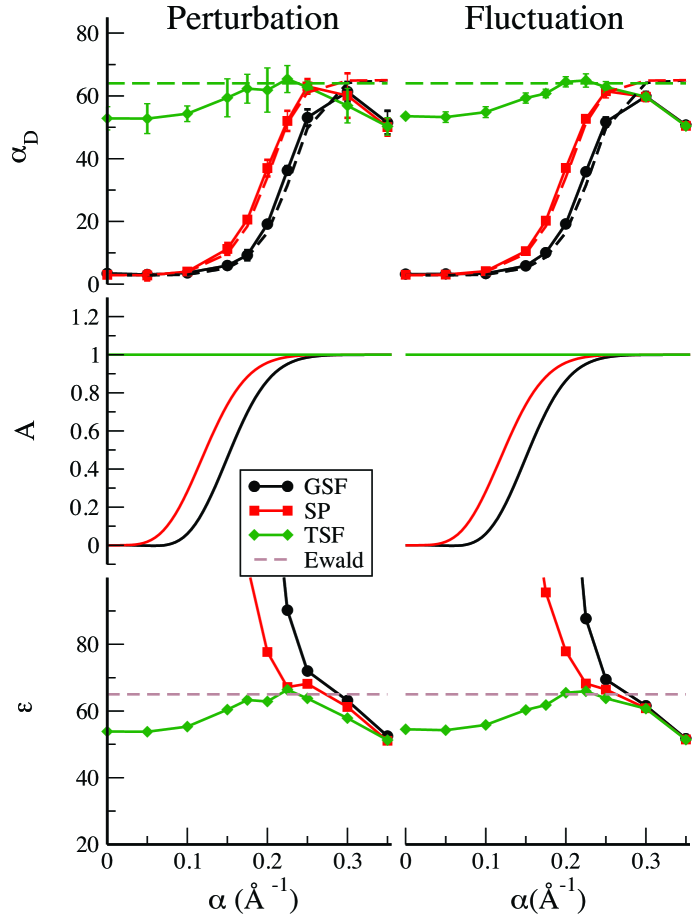
Figure 3: The polarizability ($\alpha_{D}$), correction factor ($A$), and dielectric constant ($\epsilon$) for the test dipolar fluid. The left panels were computed using external fields, and those on the right are the result of equilibrium fluctuations. In the GSF and SP methods, the corrections are large for small values of $\alpha$, and an optimal damping coefficient is evident around 0.25 Å^-1. The dashed lines in the upper panel indicate back-calculation of the polarizability using the Ewald estimate (Refs. Adams and Adams, 1981 and Neumann, 1983) for the dielectric constant.

The bulk polarizability ($\alpha_{D}$) for the dipolar fluid is shown in the upper panels in Fig. 3. The polarizability obtained from the both perturbation and fluctuation approaches are in excellent agreement with each other. The data also show a strong dependence on the damping parameter for both the Shifted Potential (SP) and Gradient Shifted force (GSF) methods, while Taylor shifted force (TSF) is largely independent of the damping parameter.

The calculated correction factors discussed in section III.3 are shown in the middle panels. Because the TSF method has $A=1$ for all values of the damping parameter, the computed polarizabilities need no correction for the dielectric calculation. The value of $A$ varies with the damping parameter in both the SP and GSF methods, and inclusion of the correction yields dielectric estimates (shown in the lower panel) that are generally too large until the damping reaches $\sim$ 0.25 Å^-1. Above this value, the dielectric constants are in reasonable agreement with previous simulation results.Neumann (1983)

Figure 3 also contains back-calculations of the polarizability using the reference (Ewald) simulation results.Neumann (1983) These are indicated with dashed lines in the upper panels. It is clear that the expected polarizability for the SP and GSF methods are quite close to results obtained from the simulations. This indicates that the correction formula for the dipolar fluid (Eq. 16) is extraordinarily sensitive when the value of $A$ deviates significantly from unity. It is also apparent that Gaussian damping is essential for capturing the field effects from other dipoles. Eq. (16) works well when real-space methods employ moderate damping, but is not capable of providing adequate correction for undamped or weakly-damped multipoles.

Because the dielectric correction in Eq. (16) is so sensitive to $A$ values away from unity, the entries in table 1 can provide an effective minimum on the values of $\alpha$ that should be used. With a minimum $A=0.995$ and a cutoff radius of 12 Å, the minimum $\alpha$ values are 0.241 Å^-1 (SP) or 0.268 Å^-1 (GSF). The TSF method is not sensitive to the choice of damping parameter.

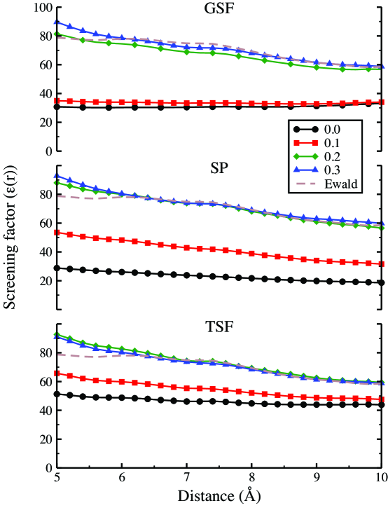
Figure 4: The distance-dependent screening factor, $\epsilon(r)$, between two ions immersed in the dipolar fluid. The new methods are shown in separate panels, and different values of the damping parameter ($\alpha$) are indicated with different symbols. All of the methods appear to be converging to the bulk dielectric constant ($\sim 65$) for higher values of $\alpha$ and at large ion separations.

We have also evaluated the distance-dependent screening factor, $\epsilon(r)$, between two oppositely charged ions when they are placed in the dipolar fluid. These results were computed using Eq. 48 and are shown in Fig. 4.

The screening factor is similar to the dielectric constant, but measures a local property of the ions in the fluid and depends on both ion-dipole and dipole-dipole interactions. These interactions depend on the distance between ions as well as the electrostatic interaction methods utilized in the simulations. The screening should converge to the dielectric constant when the field due to ions is small. This occurs when the ions are separated (or when the damping parameter is large). In Fig. 4 we observe that for the higher value of damping alpha i.e. $\alpha>0.2$ Å^-1 and large separation between ions, the screening factor does indeed approach the correct dielectric constant.

It is also notable that the TSF method again displays smaller perturbations away from the correct dielectric screening behavior. We also observe that for TSF, the method yields high dielectric screening even for lower values of $\alpha$.

At short distances, the presence of the ions creates a strong local field that acts to align nearby dipoles nearly perfectly in opposition to the field from the ions. This has the effect of increasing the effective screening when the ions are brought close to one another. This effect is present even in the full Ewald treatment, and indicates that the local ordering behavior is being captured by all of the moderately-damped real-space methods.

Distance-dependent Kirkwood factors

One of the most sensitive measures of dipolar ordering in a liquid is the disance dependent Kirkwood factor,

$$G_{K}(r)=\left<\frac{1}{N}\sum_{i}\sum_{\begin{subarray}{c}j\\ r_{ij}<r\end{subarray}}\frac{\mathbf{D}_{i}\cdot\mathbf{D}_{j}}{\left|D_{i}\right|\left|D_{j}\right|}\right>$$ (52)

which measures the net orientational (cosine) ordering of dipoles inside a sphere of radius $r$. The outer brackets denote a configurational average. Figure 5 shows $G_{K}(r)$ for the three real space methods with $r_{c}=3.52\sigma=12$ Å  and for the Ewald sum. These results were obtained from unperturbed 5 ns simulations of the dipolar fluid in the microcanonical (NVE) ensemble. For SP and GSF, the underdamped cases exhibit the “hole” at $r_{c}$ that is sometimes seen in cutoff-based method simulations of liquid water,Mark and Nilsson (2002); Fukuda et al. (2012) but for values of $\alpha>0.225$ Å^-1, agreement with the Ewald results is good.

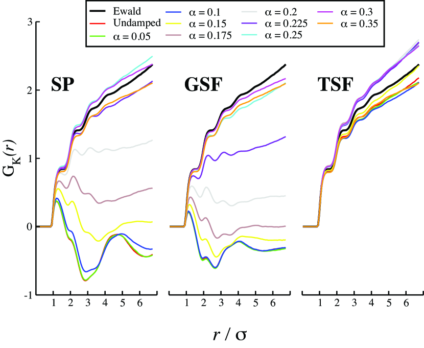
Figure 5: The distance-dependent Kirkwood factors of the dipolar system for the three real space methods at a range of Gaussian damping parameters ($\alpha$) with a cutoff $r_{c}=3.52\sigma$.

Note that like the dielectric constant, $G_{K}(r)$ can also be corrected using the expressions for $A$ in table 1. This is discussed in more detail in the supplemental material.

VII.2 Quadrupolar fluid

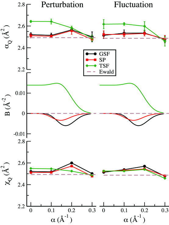
Figure 6: The quadrupole polarizability ($\alpha_{Q}$), correction factor ($B$), and susceptibility ($\chi_{Q}$) for the test quadrupolar fluid. The left panels were computed using external field gradients, and those on the right are the result of equilibrium fluctuations. The GSF and SP methods allow nearly unmodified use of the “conducting boundary” or polarizability results in place of the bulk susceptibility.

The polarizability ($\alpha_{Q}$), correction factor ($\mathrm{B}$), and susceptibility ($\chi_{Q}$) for the quadrupolar fluid is plotted against damping parameter Fig. 6. In quadrupolar fluids, both the polarizability and susceptibility have units of $\mathrm{length}^{2}$. Although the susceptibility has dimensionality, it is the relevant measure of macroscopic quadrupolar properties.Jeon and Kim (2003a, b) The left panel in Fig. 6 shows results obtained from the applied field gradient simulations whereas the results from the equilibrium fluctuation formula are plotted in the right panels.

The susceptibility for the quadrupolar fluid is obtained from quadrupolarizability and a correction factor using Eq. (44). The susceptibilities are shown in the bottom panels of Fig. 6. All three methods: (SP, GSF, and TSF) produce small correction factors, $\mathrm{B}$, so all show similar susceptibilities over the range of damping parameters. This shows that susceptibility derived using the quadrupolarizability and the correction factors are essentially independent of the electrostatic method utilized in the simulation.

There is a notable difference in the dependence on $\alpha$ for the quadrupolar correction compared with the dipolar correction. This is due to the reduced range of the quadrupole-quadrupole interaction when compared with dipolar interactions. The effects of the Gaussian damping for dipoles are significant near the cutoff radius, which can be observed in Fig. 5, while for quadrupoles, most of the interaction is naturally diminished by that point. Because overdamping can obscure orientational preferences, quadrupolar fluids can be safely simulated with smaller values of $\alpha$ than a similar dipolar fluid.

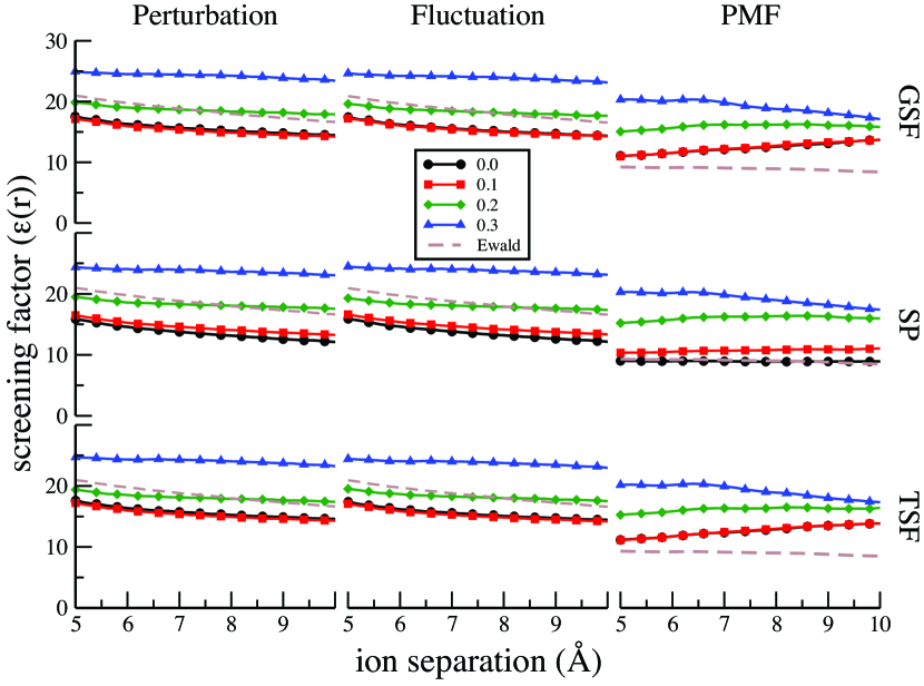
Figure 7: The distance-dependent screening factor, $\epsilon(r)$, between two ions immersed in the quadrupolar fluid. Results from the perturbation and fluctuation methods are shown in left and central panels. Here the susceptibility is calculated from the bulk simulations and the geometrical factor is evaluated using Eq. (53) using the field and field-gradient produced by the two ions. The right hand panel shows the screening factor obtained from the PMF calculations.

A more difficult test of the quadrupolar susceptibility is made by comparing with direct calculation of the electrostatic screening using the potential of mean force (PMF). Since the effective dielectric constant for a quadrupolar fluid depends on the geometry of the field and field gradient, this is not a physical property of the quadrupolar fluid.

The geometrical factor for embedded ions changes with the ion separation distance. It is therefore reasonable to treat the dielectric constant as a distance-dependent screening factor. Since the quadrupolar molecules couple with the gradient of the field, the distribution of the quadrupoles will be inhomogeneously distributed around the point charges. Hence the distribution of quadrupolar molecules should be taken into account when computing the geometrical factors in the presence of this perturbation,

$$G = \frac{\int_{V}g(\mathbf{r})\left|\nabla\mathbf{E}^{\circ}\right|^{2}d\mathbf{r}}{\int_{V}\left|\mathbf{E}^{\circ}\right|^{2}d\mathbf{r}}$$ (53)

$$= \frac{2\pi\int_{-1}^{1}\int_{0}^{R}r^{2}g(r,\cos\theta)\left|\nabla\mathbf{E}^{\circ}\right|^{2}drd(\cos\theta)}{\int_{V}\left|\mathbf{E}^{\circ}\right|^{2}d\mathbf{r}}$$

where $g(r,\cos\theta)$ is a distribution function for the quadrupoles with respect to an origin at midpoint of a line joining the two probe charges.

The effective screening factor is plotted against ion separation distance in Fig. 7. The screening evaluated from the perturbation and fluctuation methods are shown in the left and central panels. Here the susceptibilities are calculated from bulk fluid simulations and the geometrical factors are evaluated using the field and field gradients produced by the ions. The field gradients have been weighted by the $g(r,\cos\theta)$ from the PMF calculations (Eq. (53)). The right hand panel shows the screening factor obtained directly from the PMF calculations.

We note that the screening factor obtained from both the perturbation and fluctuation methods are in good agreement with each other at similar values of $\alpha$, and agree with Ewald for $\alpha=0.2$ Å^-1. The magnitude of these screening factors depends strongly on the $g(r,\cos\theta)$ weighting originating in the PMF calculations.

In Ewald-based simulations, the PMF calculations include interactions between periodic replicas of the ions, and there is a significant reduction in the screening factor because of this effect. Because the real-space methods do not include coupling to periodic replicas, both the magnitude and distance-dependent decay of the PMF are significantly larger. For moderate damping ($\alpha\sim 0.2-0.3$ Å^-1), screening factors for GSF, TSF, and SP are converging to similar values at large ion separations, and this value is the same as the large-separation estimate from the perturbation and fluctuation simulations for $\alpha\sim 0.2$ Å^-1. The PMF calculations also show signs of coalescence of the ion solvation shells at separations smaller than 7 Å. At larger separations, the $\alpha=0.2$ Å^-1 PMF calculations appear to be reproducing the bulk screening values. These results suggest that using either TSF or GSF with moderate damping is a relatively safe way to predict screening in quadrupolar fluids.

VIII Conclusions

We have used both perturbation and fluctuation approaches to evaluate dielectric properties for dipolar and quadrupolar fluids. The static dielectric constant is the relevant bulk property for dipolar fluids, while the quadrupolar susceptibility plays a similar role for quadrupoles. Corrections to both the static dielectric constant and the quadrupolar susceptibility were derived for three new real space electrostatic methods, and these corrections were tested against a third measure of dielectric screening, the potential of mean force between two ions immersed in the fluids.

For the dipolar fluids, we find that the polarizability evaluated using the perturbation and fluctuation methods show excellent agreement, indicating that equilibrium calculations of the dipole fluctuations are good measures of bulk polarizability.

One of the findings of the second paper in this series is that the moderately damped GSF and SP methods were most suitable for molecular dynamics and Monte Carlo simulations, respectively.Lamichhane, Newman, and Gezelter (2014) Our current results show that dielectic properties like $\epsilon$ and $G_{K}(r)$ are sensitive probes of local treatment of electrostatic damping for the new real space methods, as well as for the Ewald sum. Choosing a Gaussian damping parameter ($\alpha$) in a reasonable range is therefore essential for obtaining agreement between the electrostatic methods. A physical explanation of this rests on the local orientational preferences of other molecules around a central dipole. The orientational contributions to dipolar interactions are weighted by two radial functions ($v_{21}(r)$ and $v_{22}(r)$). The relative magnitudes of these functions, and therefore the orientational preferences of local dipoles, are quite sensitive to the value of $\alpha$. With moderate damping, the ratio approaches the orientational preferences of Ewald-based simulations, removing the “hole” in $G_{K}(r)$ for underdamped SP and GSF simulations (Fig. 5).

The derived correction formulae can approximate bulk properties from non-optimal parameter choices, as long as the methods are used in a relatively “safe” range of damping. The newly-derived entries in table 1 can provide an effective minimum on the values of $\alpha$ that should be used in simulations. With a cutoff radius of 12 Å, $\alpha=0.241$ Å^-1 (SP) or $0.268$ Å^-1 (GSF) would capture dielectric screening with reasonable fidelity. The sensitivity of the dielectric screening is also observed in the effective screening of ions embedded in the fluid.

With good choices of $\alpha$, the dielectric constant evaluated using the computed polarizability and correction factors agrees well with the previous Ewald-based simulation results.Adams and Adams (1981); Neumann (1983) Although the TSF method alters many dynamic and structural features in multipolar liquids,Lamichhane, Newman, and Gezelter (2014) it is surprisingly good at computing bulk dielectric properties at nearly all ranges of the damping parameter. In fact, the correction factor, $A=1$, for the TSF method so the conducting boundary formula is essentially correct when using this method for point dipolar fluids.

As in the dipolar case, the quadpole polarizability evaluated from both perturbation and fluctuation simulations show good agreement, again confirming that equilibrium fluctuation calculations are sufficient to reproduce bulk dielectric properties in these fluids. The quadrupolar susceptibility calculated via our derived correction factors produces similar results for all three real space methods. Similarly, with good choices of the damping parameter, the screening factor calculated using the susceptibility and a weighted geometric factor provides good agreement with results obtained directly via potentials of mean force. For quadrupolar fluids, the distance dependence of the electrostatic interaction is significantly reduced and the correction factors are all small. These points suggest that how an electrostatic method treats the cutoff radius become less consequential for higher order multipoles.

For this reason, our recommendation is that the moderately-damped ($\alpha=0.25-0.27$ Å^-1) GSF method is a good choice for molecular dynamics simulations where point-multipole interactions are being utilized to compute bulk dielectric properties of fluids.

Supplementary Material

See supplementary material for information on interactions with spatially varying fields, Boltzmann averages, self-contributions from quadrupoles, and corrections to distance-dependent Kirkwood factors.

Appendix A Contraction of the quadrupolar tensor with the traceless quadrupole moment

For quadrupolar liquids modeled using point quadrupoles, the interaction tensor is shown in Eq. (32). The Fourier transformation of this tensor for $\mathbf{k}=0$ is,

$$\tilde{T}_{\alpha\beta\gamma\delta}(0)=\int_{V}T_{\alpha\beta\gamma\delta}(\mathbf{r})d\mathbf{r}$$ (54)

On the basis of symmetry, the 81 elements can be placed in four different groups: $\tilde{T}_{aaaa}$, $\tilde{T}_{aaab}$, $\tilde{T}_{aabb}$, and $\tilde{T}_{aabc}$, where $a$, $b$, and $c$, and can take on distinct values from the set $\left\{x,y,z\right\}$. The elements belonging to each of these groups can be obtained using permutations of the indices. Integration of all of the elements shows that only the groups with indices ${aaaa}$ and ${aabb}$ are non-zero.

We can derive values of the components of $\tilde{T}_{aaaa}$ and $\tilde{T}_{aabb}$ as follows;

$$\tilde{T}_{xxxx}(0) = \int_{\textrm{V}}\left[3v_{41}(r)+6x^{2}v_{42}(r)/r^{2}+x^{4}\,v_{43}(r)/r^{4}\right]d\mathbf{r}$$ (55)

$$= 12\pi\int_{0}^{r_{c}}\left[v_{41}(r)+\frac{2}{3}v_{42}(r)+\frac{1}{15}v_{43}(r)\right]r^{2}\,dr=\mathrm{12\pi B}$$

and

$$\tilde{T}_{xxyy}(0) = \int_{\textrm{V}}\left[v_{41}(r)+(x^{2}+y^{2})v_{42}(r)/r^{2}+x^{2}y^{2}\,v_{43}(r)/r^{4}\right]d\mathbf{r}$$ (56)

$$= 4\pi\int_{0}^{r_{c}}\left[v_{41}(r)+\frac{2}{3}v_{42}(r)+\frac{1}{15}v_{43}(r)\right]r^{2}\,dr=\mathrm{4\pi B}.$$

These integrals yield the same values for all permutations of the indices in both tensor element groups. In Eq. 37, for a particular value of the quadrupolar polarization $\tilde{\Theta}_{aa}$ we can contract $\tilde{T}_{aa\gamma\delta}(0)$ with $\tilde{\Theta}_{\gamma\delta}$, using the traceless properties of the quadrupolar moment,

$$\tilde{T}_{xx\gamma\delta}(0)\tilde{\Theta}_{\gamma\delta}(0) = \tilde{T}_{xxxx}(0)\tilde{\Theta}_{xx}(0)+\tilde{T}_{xxyy}(0)\tilde{\Theta}_{yy}(0)+\tilde{T}_{xxzz}(0)\tilde{\Theta}_{zz}(0)$$ (57)

$$= 12\pi\mathrm{B}\tilde{\Theta}_{xx}(0)+4\pi\mathrm{B}\tilde{\Theta}_{yy}(0)+4\pi\mathrm{B}\tilde{\Theta}_{zz}(0)$$

$$= 8\pi\mathrm{B}\tilde{\Theta}_{xx}(0)+4\pi\mathrm{B}\left(\tilde{\Theta}_{xx}(0)+\tilde{\Theta}_{yy}(0)+\tilde{\Theta}_{zz}(0)\right)$$

$$= 8\pi\mathrm{B}\tilde{\Theta}_{xx}(0)$$

Similarly for a quadrupolar polarization $\tilde{\Theta}_{xy}$ in Eq. 37, we can contract $\tilde{T}_{xy\gamma\delta}(0)$ with $\tilde{\Theta}_{\gamma\delta}$, using the only surviving terms of the tensor,

$$\tilde{T}_{xy\gamma\delta}(0)\tilde{\Theta}_{\gamma\delta}(0) = \tilde{T}_{xyxy}(0)\tilde{\Theta}_{xy}(0)+\tilde{T}_{xyyx}(0)\tilde{\Theta}_{yx}(0)$$ (58)

$$= 4\pi\mathrm{B}\tilde{\Theta}_{xy}(0)+4\pi\mathrm{B}\tilde{\Theta}_{yx}(0)$$

$$= 8\pi\mathrm{B}\tilde{\Theta}_{xy}(0)$$

Here, we have used the symmetry of the quadrupole tensor to combine the symmetric terms. Therefore we can write matrix contraction for $\tilde{T}_{\alpha\beta\gamma\delta}(\mathrm{0})$ and $\tilde{\Theta}_{\gamma\delta}(\mathrm{0})$ in a general form,

$$\tilde{T}_{\alpha\beta\gamma\delta}(\mathrm{0})\tilde{\Theta}_{\gamma\delta}(\mathrm{0})=8\pi\mathrm{B}\tilde{\Theta}_{\alpha\beta}(\mathrm{0}),$$ (59)

which is the same as Eq. (38).

When the molecular quadrupoles are represented by point charges, the symmetry of the quadrupolar tensor is same as for point quadrupoles (see Eqs. 29 and 32). However, for molecular quadrupoles represented by point dipoles, the symmetry of the quadrupolar tensor must be handled separately (compare Eqs. 31 and 32). Although there is a difference in symmetry, the final result (Eq. 59) also holds true for dipolar representations.

Appendix B Quadrupolar correction factor for the Ewald-Kornfeld (EK) method

The interaction tensor between two point quadrupoles in the Ewald method may be expressed,Smith (1998); Neumann and Steinhauser (1983)

$${T}_{\alpha\beta\gamma\delta}(\mathbf{r})= \frac{4\pi}{V}\sum_{k\neq 0}^{\infty}e^{-k^{2}/4\kappa^{2}}e^{-i\mathbf{k}\cdot\mathbf{r}}\left(\frac{r_{\alpha}r_{\beta}k_{\delta}k_{\gamma}}{k^{2}}\right)$$

$$+\left(\delta_{\alpha\beta}\delta_{\gamma\delta}+\delta_{\alpha\gamma}\delta_{\beta\delta}+\delta_{\alpha\delta}\delta_{\beta\gamma}\right)B_{2}(r)$$

$$-\left(\delta_{\gamma\delta}r_{\alpha}r_{\beta}+\mathrm{5\;permutations}\right)B_{3}(r)$$

$$+\left(r_{\alpha}r_{\beta}r_{\gamma}r_{\delta}\right)B_{4}(r)$$ (60)

where $B_{n}(r)$ are radial functions defined in reference Smith, 1998,

$$B_{2}(r)= \frac{3}{r^{5}}\left(\frac{2r\kappa e^{-r^{2}\kappa^{2}}}{\sqrt{\pi}}+\frac{4r^{3}\kappa^{3}e^{-r^{2}\kappa^{2}}}{3\sqrt{\pi}}+\mathrm{erfc(\kappa r)}\right)$$ (61)

$$B_{3}(r)= -\frac{15}{r^{7}}\left(\frac{2r\kappa e^{-r^{2}\kappa^{2}}}{\sqrt{\pi}}+\frac{4r^{3}\kappa^{3}e^{-r^{2}\kappa^{2}}}{3\sqrt{\pi}}+\frac{8r^{5}\kappa^{5}e^{-r^{2}\kappa^{2}}}{15\sqrt{\pi}}+\mathrm{erfc(\kappa r)}\right)$$ (62)

$$B_{4}(r)= \frac{105}{r^{9}}\left(\frac{2r\kappa e^{-r^{2}\kappa^{2}}}{\sqrt{\pi}}+\frac{4r^{3}\kappa^{3}e^{-r^{2}\kappa^{2}}}{3\sqrt{\pi}}+\frac{8r^{5}\kappa^{5}e^{-r^{2}\kappa^{2}}}{15\sqrt{\pi}}+\frac{16r^{7}\kappa^{7}e^{-r^{2}\kappa^{2}}}{105\sqrt{\pi}}+\mathrm{erfc(\kappa r)}\right)$$ (63)

We can divide ${T}_{\alpha\beta\gamma\delta}(\mathbf{r})$ into three parts:

$$\mathbf{T}(\mathbf{r})=\mathbf{T}^{\mathrm{K}}(\mathbf{r})+\mathbf{T}^{\mathrm{R1}}(\mathbf{r})+\mathbf{T}^{\mathrm{R2}}(\mathbf{r})$$ (64)

where the first term is the reciprocal space portion. Since the quadrupolar correction factor $B=\tilde{T}_{abab}(0)/4\pi$ and $\mathbf{k}=0$ is excluded from the reciprocal space sum, $\mathbf{T}^{\mathrm{K}}$ will not contribute.Neumann and Steinhauser (1983) The remaining terms,

$$\mathbf{T}^{\mathrm{R1}}(\mathbf{r})=\mathbf{T}^{\mathrm{bare}}(\mathbf{r})\left(\frac{2r\kappa e^{-r^{2}\kappa^{2}}}{\sqrt{\pi}}+\frac{4r^{3}\kappa^{3}e^{-r^{2}\kappa^{2}}}{3\sqrt{\pi}}+\frac{8r^{5}\kappa^{5}e^{-r^{2}\kappa^{2}}}{15\sqrt{\pi}}+\frac{16r^{7}\kappa^{7}e^{-r^{2}\kappa^{2}}}{105\sqrt{\pi}}+\mathrm{erfc(\kappa r)}\right)$$ (65)

and

$$T^{\mathrm{R2}}_{\alpha\beta\gamma\delta}(\mathbf{r})= + \left(\delta_{\gamma\delta}r_{\alpha}r_{\beta}+\mathrm{5\;permutations}\right)\frac{16\kappa^{7}e^{-r^{2}\kappa^{2}}}{7\sqrt{\pi}}$$ (66)

$$- \left(\delta_{\alpha\beta}\delta_{\gamma\delta}+\delta_{\alpha\gamma}\delta_{\beta\delta}+\delta_{\alpha\delta}\delta_{\beta\gamma}\right)\left(\frac{8\kappa^{5}e^{-r^{2}\kappa^{2}}}{5\sqrt{\pi}}+\frac{16r^{2}\kappa^{7}e^{-r^{2}\kappa^{2}}}{35\sqrt{\pi}}\right)$$

are contributions from the real space sum.Adams and McDonald (1976); Adams (1980); Adams and Adams (1981) Here $\mathbf{T}^{\mathrm{bare}}(\mathbf{r})$ is the unmodified quadrupolar tensor (for undamped quadrupoles). Due to the angular symmetry of the unmodified tensor, the integral of $\mathbf{T}^{\mathrm{R1}}(\mathbf{r})$ will vanish when integrated over a spherical region. The only term contributing to the correction factor (B) is therefore $T^{\mathrm{R2}}_{\alpha\beta\gamma\delta}(\mathbf{r})$, which allows us to derive the correction factor for the Ewald-Kornfeld (EK) method,

$$\mathrm{B} = \frac{1}{4\pi}\int_{V}T^{\mathrm{R2}}_{abab}(\mathbf{r})$$ (67)

$$= -\frac{8r_{c}^{3}\kappa^{5}e^{-\kappa^{2}r_{c}^{2}}}{15\sqrt{\pi}}.$$

References

- Wolf et al. (1999) D. Wolf, P. Keblinski, S. R. Phillpot, and J. Eggebrecht, J. Chem. Phys. 110, 8254 (1999).
- Zahn, Schilling, and Kast (2002) D. Zahn, B. Schilling, and S. M. Kast, J. Phys. Chem. B 106, 10725 (2002).
- Kast, Schmidt, and Schilling (2003) S. M. Kast, K. F. Schmidt, and B. Schilling, Chem. Phys. Lett. 367, 398 (2003).
- Beck, Armen, and Daggett (2005) D. Beck, R. Armen, and V. Daggett, Biochemistry 44, 609 (2005).
- Ma and Garofalini (2005) Y. Ma and S. H. Garofalini, Mol. Simul. 31, 739 (2005).
- Wu and Brooks (2005) X. Wu and B. R. Brooks, J. Chem. Phys. 122, 044107 (2005).
- Fennell and Gezelter (2006) C. J. Fennell and J. D. Gezelter, J. Chem. Phys. 124, 234104 (2006).
- Fukuda (2013) I. Fukuda, J. Chem. Phys. 139, 174107 (2013).
- Stenqvist et al. (2015) B. Stenqvist, M. Trulsson, A. I. Abrikosov, and M. Lund, J. Chem. Phys. 143, 014109 (2015).
- Wang, Nakamura, and Fukuda (2016) H. Wang, H. Nakamura, and I. Fukuda, J. Chem. Phys. 144, 114503 (2016).
- Lamichhane, Gezelter, and Newman (2014) M. Lamichhane, J. D. Gezelter, and K. E. Newman, J. Chem. Phys. 141, 134109 (2014).
- Lamichhane, Newman, and Gezelter (2014) M. Lamichhane, K. E. Newman, and J. D. Gezelter, J. Chem. Phys. 141, 134110 (2014).
- Kirkwood (1939) J. G. Kirkwood, J. Chem. Phys. 7, 911 (1939).
- Onsager (1936) L. Onsager, J. Am. Chem. Soc. 58, 1486 (1936).
- Chitanvis (1996) S. M. Chitanvis, J. Chem. Phys. 104, 9065 (1996).
- Stern and Feller (2003) H. A. Stern and S. E. Feller, J. Chem. Phys. 118, 3401 (2003).
- Slavchov and Ivanov (2014) R. I. Slavchov and T. I. Ivanov, J. Chem. Phys. 140, 074503 (2014).
- Slavchov (2014) R. I. Slavchov, J. Chem. Phys. 140, 164510 (2014).
- Neumann (1983) M. Neumann, Mol. Phys. 50, 841 (1983).
- Neumann and Steinhauser (1983) M. Neumann and O. Steinhauser, Chem. Phys. Lett. 95, 417 (1983).
- Izvekov, Swanson, and Voth (2008) S. Izvekov, J. M. J. Swanson, and G. A. Voth, J. Phys. Chem. B 112, 4711 (2008).
- Ernst et al. (1992) R. M. Ernst, L. Wu, C.-h. Liu, S. R. Nagel, and M. E. Neubert, Phys. Rev. B 45, 667 (1992).
- Jeon and Kim (2003a) J. Jeon and H. J. Kim, J. Chem. Phys. 119, 8606 (2003a).
- Jeon and Kim (2003b) J. Jeon and H. J. Kim, J. Chem. Phys. 119, 8626 (2003b).
- Neumann, Steinhauser, and Pawley (1984) M. Neumann, O. Steinhauser, and G. S. Pawley, Mol. Phys. 52, 97 (1984).
- Neumann (1985) M. Neumann, J. Chem. Phys. 82, 5663 (1985).
- Adams (1980) D. Adams, Mol. Phys. 40, 1261 (1980).
- Adams and Adams (1981) D. Adams and E. Adams, Mol. Phys. 42, 907 (1981).
- Adu-Gyamfi (1978) D. Adu-Gyamfi, Physica A 93, 553 (1978).
- Adu-Gyamfi (1981) D. Adu-Gyamfi, Physica A 108, 205 (1981).
- Logan (1981) D. E. Logan, Mol. Phys. 44, 1271 (1981).
- Logan (1982a) D. E. Logan, Mol. Phys. 46, 271 (1982a).
- Logan (1982b) D. E. Logan, Mol. Phys. 46, 1155 (1982b).
- Trzesniak, Kunz, and van Gunsteren (2007) D. Trzesniak, A.-P. E. Kunz, and W. F. van Gunsteren, ChemPhysChem 8, 162 (2007).
- Fixman (1974) M. Fixman, Proc. Natl. Acad. Sci. USA 71, 3050 (1974).
- Smith (1982) W. Smith, CCP5 Information Quarterly 4, 13 (1982).
- Smith (1998) W. Smith, CCP5 Information Quarterly 46, 18 (1998).
- Meineke et al. (2005) M. A. Meineke, C. F. Vardeman II, T. Lin, C. J. Fennell, and J. D. Gezelter, J. Comp. Chem. 26, 252 (2005).
- Gezelter et al. (2016) J. D. Gezelter, M. Lamichhane, J. Michalka, P. Louden, K. M. Stocker, S. Kuang, J. Marr, C. Li, C. F. Vardeman, T. Lin, C. J. Fennell, X. Sun, K. Daily, Y. Zheng, and M. A. Meineke, OpenMD (An open source molecular dynamics engine, version 2.4, http://openmd.org (accessed 4/8/2016)).
- Mark and Nilsson (2002) P. Mark and L. Nilsson, J. Comp. Chem. 23, 1211 (2002).
- Fukuda et al. (2012) I. Fukuda, N. Kamiya, Y. Yonezawa, and H. Nakamura, The Journal of Chemical Physics 137, 054314 (2012).
- Adams and McDonald (1976) D. J. Adams and I. R. McDonald, Mol. Phys. 32, 931 (1976).