Superiorization of Incremental Optimization Algorithms for Statistical Tomographic Image Reconstruction

Abstract

We propose the superiorization of incremental algorithms for tomographic image reconstruction. The resulting methods follow a better path in its way to finding the optimal solution for the maximum likelihood problem in the sense that they are closer to the Pareto optimal curve than the non-superiorized techniques. A new scaled gradient iteration is proposed and three superiorization schemes are evaluated. Theoretical analysis of the methods as well as computational experiments with both synthetic and real data are provided.

1 Introduction

Tomographic images reconstructed from projection data are important tools in various applications, for example, ranging from medicine to materials science and from geosciences to astronomy. It is therefore useful to develop the techniques that enable good reconstruction from a variety of data acquisition modalities. That means being able to cope with statistical error, poor angular sampling, truncated data, among other difficulties. Sometimes a combination of factors must be dealt with.

Statistical methods were developed in order to handle poor photon counts, mainly for use in emission tomography modalities. Among those we can mention, in order of appearance, em [13, 15], os-em [10], ramla [2], bsrem [4], drama [14, 8] and saem [7]. The original numerical approach to solve the statistical optimization model was the em algorithm, which was deemed too slow, taking many iterations to provide reasonably accurate images; os-em subdivides the data into subsets and processes each of these incrementally in order to achieve an order of magnitude speedup compared to em, but leads to oscillatory behavior when applied to inconsistent data; ramla takes the subset approach to the extreme using a single datum at a time, but prevents oscillation through the use of relaxation in order to ensure convergence; bsrem generalizes ramla by considering more flexible subset divisions and by allowing the use of regularization in the objective function; drama introduced variable relaxation within an iteration cycle aiming at a more even noise contribution from each individual datum in the resulting images; finally, saem further enhance the possibilities by considering a parallelization approach whereby the same algorithm is applied in parallel to subsets of the data and the results are averaged to form the next iterate.

In the present paper, we consider yet another direction for statistical methods. All of the aforementioned algorithms use a diagonal scaling of the descent direction, which provides desirable convergence characteristics and and helps in maintaining non-negativity of the iterations. This diagonal scaling has the drawback of making convergence analysis more difficult in the case of a non-differentiable objective function, which precludes several useful regularization functions. We, therefore, make use of the superiorization framework in order to analyze algorithms for this case. Our analysis will cover all of the above cited methods, allowing for the use of more interesting regularization functions alongside scaled incremental algorithms for the statistical tomographic reconstruction problem. Moreover, we present a new algorithmic framework which has better theoretical characteristics than the techniques mentioned in the previous paragraph, with similar practical performance.

We use both the superiorized saem algorithm and the newly presented superiorized approach in order to solve real world tomographic problems arising from synchrotron illuminated radiographic data. Implementation of the techniques was very inhomogeneous with the former being implemented using Matlab and the second running on gpus, so no direct comparison was intended to be made.

1.1 Tomographic Imaging from Projections

The most common transmission tomography technique makes use of x-rays, based on the Beer-Lambert law:

$$\frac{I_{d}}{I_{e}}=e^{-\int_{L}\mu(\boldsymbol{x})\mathrm{d}s},$$ (1)

where $I_{d}$ and $I_{e}$ are, respectively, the detected and the emitted x-ray beam intensities, $L$ is the line segment connecting emitter and detector and $\mu:\mathbb{R}^{2}\to\mathbb{R}_{+}$ is the non-negative linear attenuation factor. Different attenuation factor values usually correspond to features of interest, for example, the body anatomy in human patients, and therefore its knowledge brings important information for applications. The problem is now to recover the attenuation factor $\mu$ at each point in the plane from the non-invasive measurements of line integrals of $\mu$. While, for simplicity of exposition, we focus the two dimensional case in the present paper, volumetric images can be obtained either by stacking planar tomographic images or by directly extending the approach to 3D datasets.

We simplify the notation by parameterizing the data by the angle $\theta$ between the normal to the integration path and the horizontal axis and by the distance $t$ of this integration path to the origin of the coordinate system. In doing so, we define the Radon transform $\mathcal{R}$, which takes functions on the plane to functions on the cylinder as follows:

$$\mathcal{R}[\mu](\theta,t):=\int_{\mathbb{R}}\mu\left(t\left(\begin{smallmatrix}\cos\theta\\ \sin\theta\end{smallmatrix}\right)+s\left(\begin{smallmatrix}-\sin\theta\\ \cos\theta\end{smallmatrix}\right)\right)\mathrm{d}s.$$ (2)

Figure 1: Left: meaning of the arguments of the Radon transform. Here, $\theta$ is the angle between the normal to the integration path and the horizontal axis, and $t$ is the distance from the line of integration to the origin. Right: sinogram, i.e., an image of the Radon transform of the image shown on the left in the $\theta\times t$ coordinate system (adapted from [7]).

Figure 1 depicts this definition. The Radon transform is mathematically rich, possessing several useful properties. Among those we can mention, for example, the Fourier slice property, which relates the one-dimensional Fourier transforms of $\mathcal{R}[\mu]$ along the $t$ coordinate to “slices” of the two-dimensional Fourier transform of the image $\mu$. More importantly for us here, the Radon transform turns out to be a compact linear operator which has, in consequence, an ill-conditioned inverse or pseudo-inverse [11].

1.2 Iterative Image Reconstruction

While exploring some deep mathematical properties of the Radon transform can lead to useful inversion formulas, sometimes it is better to consider all of the involved physical effects more carefully. For example, the observation that the emission of photons follows a stochastic rule can lead to improved imaging by the introduction of maximum likelihood models whereby the reconstructed image is selected as the one that would give the maximum possible likelihood for the observed data. Whichever the imaging modality is, this approach will give rise to an optimization problem to be solved, therefore bringing the need to use iterative algorithms in order to approximate the solution of the model.

In every optimization model, whether based on statistical ideas or not, a discretization of the imaged object has to be taken into consideration and, given the finite nature of the data, the Radon transform, or more physically precise stripe-based integral transforms, can be represented by a matrix $R\in\mathbb{R}^{m\times n}$. In this setting, the image is written as

$$\sum_{j=1}^{n}x_{j}\mu_{j},$$

where $\{\mu_{1},\mu_{2},\dots,\mu_{n}\}$ is a basis for the space where the imaged object is assumed to be and $x_{j}$ are the components of vector $\boldsymbol{x}\in\mathbb{R}^{n}$. In all of our models, the basis will be the indicator functions of square pixels which also means that the $x_{j}$ are the actual values of the pixelized image. If taken literally, the problem would then become to find the solution of the linear system of equations

$$R\boldsymbol{x}=\boldsymbol{b},$$

where the coefficients of $R$ are $r_{ij}=\mathcal{R}[\mu_{j}](\theta_{i},t_{i})$ and the components of $\boldsymbol{b}$ are approximations to the Radon transform: $b_{i}\approx\mathcal{R}[\mu](\theta_{i},t_{i})$, where $\mu$ is the desired true image. The system matrix arising in tomographic problems ranges from mildly to severely ill-posed, which brings difficulties because of the experimental error in the collected tomographic data $\boldsymbol{b}$.

Therefore, instead of directly solving the above linear system of equations, it is usually more profitable to consider a (regularized) maximum likelihood model. For example, in emission tomography the desired image is the intensity of photon emission across the imaged plane, i.e., the number of emitted photons on each square pixel [15]. In his case, maximizing the likelihood of obtaining the data is equivalent to solve the following optimization problem:

$$\begin{split}\min&\quad L_{\textsc{e}}(\boldsymbol{x}):=\sum_{i=1}^{m}\left\{(R\boldsymbol{x})_{i}-b_{i}\ln(R\boldsymbol{x})_{i}\right\}\\ \operatorname{s.t.:}&\quad\boldsymbol{x}\in\mathbb{R}_{+}^{n},\end{split}$$

where, in this case, $b_{i}$ represents the attenuation corrected number of photons detected on bin $i$.

For the case of transmission tomography, if we denote as $\rho_{i}$ the number of events detected by detector $i$ during a dark scan (i.e., no x-ray source turned on), $\beta_{i}$ to be the number of photons detected by detector $i$ during a blank scan and $\alpha_{i}$ the number of photons detected by detector $i$ during the actual tomographic scan of the object, the maximum likelihood problem is equivalent to [12]:

$$\begin{split}\min&\quad L_{\textsc{tr}}(\boldsymbol{x}):=\sum_{i=1}^{m}\left\{\beta_{i}e^{-(R\boldsymbol{x})_{i}}-\alpha_{i}\log\left(e^{-(R\boldsymbol{x})_{i}}+\rho_{i}\right)\right\}\\ \operatorname{s.t.:}&\quad\boldsymbol{x}\in\mathbb{R}_{+}^{n}.\end{split}$$

Both of the above functions are convex [9] (convexity of $L_{\textsc{tr}}$ requires assumptions on the data which are always satisfied in practice), although not always strictly convex. Non-convex models do exist for the tomographic imaging problem, but due to the usually large dimensions of the problem algorithms for the convex optimization problem are more practical and much more common in practice. We will focus only on convex models in the present paper. In the next section we present the proposed algorithms and the general optimization model they intend to solve.

2 Algorithm Description

For optimization problems like

$$\begin{split}\min&\quad f(\boldsymbol{x})\\ \operatorname{s.t.:}&\quad\boldsymbol{x}\in\mathbb{R}_{+}^{n},\end{split}$$ (3)

with $f:\mathbb{R}^{n}\to\mathbb{R}$ convex and differentiable, we will consider algorithms of the form

$$\boldsymbol{x}^{(k+1)}=\boldsymbol{x}^{(k)}-\lambda_{k}D(\boldsymbol{x}^{(k)})\nabla f(\boldsymbol{x}^{(k)})+\boldsymbol{\epsilon}^{(k)},$$ (4)

where the diagonal scaling matrix will be given differently according to one of two algorithmic schemes to be described later. Furthermore, it is assumed that

$$\lambda_{k}>0,\quad\sum_{k=0}^{\infty}\lambda_{k}=\infty.$$

For us, the usefulness of allowing the error sequence $\{\boldsymbol{\epsilon}^{(k)}\}$ in the analysis will be twofold. First, as already observed before in the literature [2, 4, 8, 7], it allows for flexible, from sequential to parallel with many intermediate instances, processing of the data giving rise to fast and stable algorithms. Second, it will allow us to apply the superiorization concept in order to drive the iterates to the optimum through a path with smoother intermediate iterates, as follows. We write an algorithm following (4) in a compact form as

$$\boldsymbol{x}^{(k+1)}=\mathcal{O}(\lambda_{k},\boldsymbol{x}^{(k)}),$$ (5)

and we create a new algorithm following

$$\boldsymbol{x}^{(k+1)}=\tilde{\mathcal{O}}(\lambda_{k},\boldsymbol{x}^{(k)}):=\mathcal{O}(\lambda_{k},\boldsymbol{x}^{(k)})+\boldsymbol{s}^{(k)},$$ (6)

where we name $\{\boldsymbol{s}^{(k)}\}$ the superiorization sequence. Algorithm (6) is correspondingly named the superiorized version of Algorithm (4). Notice that if we define $\tilde{\boldsymbol{\epsilon}}^{(k)}:=\boldsymbol{\epsilon}^{(k)}+\boldsymbol{s}^{(k)}$, we then have that iterations (6) are equivalent to

$$\boldsymbol{x}^{(k+1)}=\boldsymbol{x}^{(k)}-\lambda_{k}D(\boldsymbol{x}^{(k)})\nabla f(\boldsymbol{x}^{(k)})+\tilde{\boldsymbol{\epsilon}}^{(k)}.$$

That is, the essential approximation characteristics of the method are not ruined by adding a deliberate, appropriately small, perturbation. We shall worry about convergence issues in the next section.

In the remainder of the present section we describe two options for the operator $\mathcal{O}$, one of which is an existing algorithm while the second is our new proposal. Furthermore, we also describe more precisely the two alternatives for the superiorization sequence we will try in the numerical section.

2.1 String-Averaging Expectation Maximization

The String-Averaging Expectation Maximization (saem) algorithm was introduced in [7] and applied to a maximum likelihood problem in tomographic reconstruction. Convergence analysis contained in [7] embraces somewhat general smooth convex cost functions, and therefore we will keep the acronym saem even when not necessarily referring to applications to likelihood maximization problems.

In order to describe saem, we assume that the objective function can be written as:

$$f(\boldsymbol{x})=\sum_{i=1}^{p}f_{i}(\boldsymbol{x}),$$

where $f:\mathbb{R}^{n}\to\mathbb{R}$ is supposed to be a convex function and $f_{i}:\mathbb{R}^{n}\to\mathbb{R}$ are sufficiently smooth functions.

We then assume that the sequence $\{1,2,\dots,p\}$ is split in $s$ (ordered) subsets, $\{S_{1},S_{2},\dots,S_{s}\}$, each of which is called a string, satisfying

$$\bigcup_{l=1}^{s}S_{l}=\{1,2,\dots,p\}\quad\text{and}\quad S_{l}\cap S_{\ell}=\emptyset\quad\forall l\neq\ell.$$

We make each of the subsets explicit through the following notation for the elements of each string:

$$S_{l}:=\{\iota^{l}_{1},\iota^{l}_{2},\dots,\iota^{l}_{\nu(l)}\}.$$

That is, $\iota^{l}_{i}$ is the $i^{\text{th}}$ element of string $S_{l}$ and $\nu(l)$ is the cardinality of string $S_{l}$.

Now, for each string we iterate a scaled incremental gradient for the function $F_{l}:=\sum_{i\in S_{l}}f_{i}$. Let us define the string operators $\mathcal{S}_{l}:\mathbb{R}\times\mathbb{R}^{n}\to\mathbb{R}^{n}$ for this purpose:

$$\mathcal{S}_{l}(\lambda,\boldsymbol{x}):=\boldsymbol{y}^{(\nu(l))},$$

where $\lambda$ is a positive scalar, $\boldsymbol{x}\in\mathbb{R}^{n}$ and the vectors $\boldsymbol{y}^{(i)}\in\mathbb{R}^{n}$, $i\in\{1,2,\dots,\nu(l)\}$ are recursively computed from the identity below:

$$\boldsymbol{y}^{(i)}=\boldsymbol{y}^{(i-1)}-\lambda D(\boldsymbol{y}^{(i-1)})\nabla f_{\iota^{l}_{i}}(\boldsymbol{y}^{(i-1)}),\quad i\in\{1,2,\dots,\nu(l)\}.$$

Recursion starts from $\boldsymbol{y}^{(0)}=\boldsymbol{x}$, and the scaling matrix is given by

$$D(\boldsymbol{x}):=\begin{pmatrix}\displaystyle\frac{x_{1}}{p_{1}}&&&&\\ &\displaystyle\frac{x_{2}}{p_{2}}&&\\ &&\ddots&\\ &&&\displaystyle\frac{x_{n}}{p_{n}}\end{pmatrix},$$ (7)

where $p_{j}>0$ and $x_{1},x_{2},\dots,x_{n}$ are the components of $\boldsymbol{x}$.

Each of these operators is no more than a block-ramla (bramla) iteration over a specific data subset [2, 4]. A bramla iteration is a generalization of a ramla iteration whereby blocks of data can be used at each subiteration. Under mild smoothness assumptions on the gradients $\nabla f_{i}$, it is possible to show that

$$\mathcal{S}_{l}(\lambda,\boldsymbol{x})=\boldsymbol{x}-\lambda D(\boldsymbol{x})\nabla F_{l}(\boldsymbol{x})+O(\lambda^{2}).$$

See, e.g., [7, Proposition 5.3]. Therefore, by setting weights $\{\omega_{1},\omega_{2},\dots,\omega_{s}\}$ such that $\sum_{l=1}^{s}\omega_{l}=1$ and $\omega_{l}\geq 0$, we can finally define the iterative procedure:

$$\boldsymbol{x}^{(k+1)}=\sum_{l=1}^{s}\omega_{l}\mathcal{S}_{l}(\boldsymbol{x}^{(k)},\lambda_{k}).$$

For which, then, there holds

$$\boldsymbol{x}^{(k+1)}=\boldsymbol{x}^{(k)}-\lambda_{k}\nabla\tilde{f}(\boldsymbol{x}_{k})+O(\lambda_{k}^{2}),$$

where $\tilde{f}:=\sum_{l=1}^{s}\omega_{l}F_{l}$ is a weighted version of the original objective function $f=\sum_{l=1}^{s}F_{l}$.

A key, albeit very simple, observation here is that the convergence analysis naturally absorbs an error term, which makes it attractive for the superiorization approach because we can add suitable perturbations to this error term and still maintain a convergent algorithm. In order to do that, the magnitude of the perturbation must be appropriately controlled, which we will analyze theoretically in depth in the next section. The remaining of the present section presents an option to saem and then discusses the three forms of the perturbation $\{\boldsymbol{s}^{(k)}\}$ we consider, which we recall that we have named superiorization sequences.

2.2 New Superiorized Scaled Gradient Algorithm

In the present paper, we not only introduce superiorization of well known maximum likelihood algorithms, but we also present a different method with improved theoretical characteristics when compared to ramla and its relatives, while maintaining the good practical performance of these techniques. In order to describe the new algorithmic framework, there is a key idea: that the diagonal scaling matrix cannot have components vanishing when the corresponding entry in the gradient is positive, in order to avoid the possibility of convergence to a non-optimal point when the objective function is convex but not strictly convex. Of course the precise way of interpreting and implementing this statement is very important to the final computational results, and we describe it in details below.

In the following description we use the same notation for the strings given in Section 2.1. The concrete algorithm that we propose uses strings similarly to saem, but is stabilized in a sense that it actually approximates a better-scaled iteration. We name it ssaem from Stabilized saem, and the iterations are as follows:

$$\tilde{\mathcal{S}}_{l}(\lambda_{k},\boldsymbol{x}^{(k)}):=\boldsymbol{y}^{(k,l,\nu(l))},$$

where

$$\boldsymbol{y}^{(k,l,i)}=\boldsymbol{y}^{(k,l,i-1)}-\lambda_{k}\overline{D}(\boldsymbol{y}^{(k,l,i-1)})\nabla f_{\iota^{l}_{i}}(\boldsymbol{y}^{(k,l,i-1)}),\quad i\in\{1,2,\dots,\nu(l)\},$$

and

$$\boldsymbol{y}^{(k,0)}=\boldsymbol{x}^{(k)}.$$

The diagonal scaling matrix $\overline{D}$ is given componentwise, for $\boldsymbol{x}\in\mathbb{R}_{+}^{n}$, by

$$\overline{D}(\boldsymbol{x})_{jj}:=\begin{cases}\frac{x_{j}}{p_{j}}&\text{if}\quad x_{j}>\tau\\ \frac{\tau}{p_{j}}&\text{otherwise,}\end{cases}$$

where each $p_{j}$, $j\in\{1,2,\dots,n\}$ is positive.

The next iterate is computed in two steps. First the averaging:

$$\boldsymbol{\tilde{x}}^{(k+1)}=\sum_{l=1}^{s}\omega_{l}\tilde{\mathcal{S}}_{l}(\lambda_{k},\boldsymbol{x}^{(k)}).$$

and then a componentwise correction:

$$x^{(k+1)}_{j}=\begin{cases}x^{(k)}_{j}+\frac{x^{(k)}_{j}}{\tau}\left(\tilde{x}^{(k+1)}_{j}-x^{(k)}_{j}\right)&\text{if}\quad x^{(k)}_{j}\leq\tau\quad\text{and}\quad\tilde{x}^{(k+1)}_{j}<x^{(k)}_{j}\\ \tilde{x}^{(k+1)}_{j}&\text{otherwise.}\\ \end{cases}$$

We discuss some useful facts about these iterations in preparation for the complete convergence analysis to be provided in the next section.

Proposition 1.

Fix $l\in\{1,2,\dots,s\}$. Suppose that $x^{(k)}_{j}\geq 0$ for all $j\in\{1,2,\dots,n\}$, and that, for every $i\in\{1,2,\dots,\nu(l)\}$, $\{\nabla f_{\iota^{l}_{i}}(\boldsymbol{y}^{(k,l,i-1)})\}_{k\in\mathbb{N}}$ is bounded, $\nabla f_{\iota^{l}_{i}}$ is Lipschitz in

$$C_{l,i}:=\text{the closure of the convex hull of }\{\boldsymbol{x}^{(k)},\boldsymbol{y}^{(k,l,i-1)}\}_{k\in\mathbb{N}},$$

and that $C_{l,i}$ is in turn bounded. Then:

$$\tilde{\mathcal{S}}_{l}(\lambda_{k},\boldsymbol{x}^{(k)})=\boldsymbol{x}^{(k)}-\lambda_{k}\overline{D}(\boldsymbol{x}^{(k)})\left(\nabla F_{l}(\boldsymbol{x}^{(k)})+O(\lambda_{k})\right).$$

Proof.

Notice that the hypothesis ensure that each function $\overline{D}(\cdot)\nabla f_{\iota^{l}_{i}}(\cdot)$ is Lipschitz, say with Lipschitz constant $M$, in $C_{i}$ and thus, if we define

$$\begin{split}\boldsymbol{\epsilon}^{(k,l)}&{}:=\overline{D}(\boldsymbol{x}^{(k)})\nabla F_{l}(\boldsymbol{x}^{(k)})-\sum_{i=1}^{\nu(l)}\overline{D}(\boldsymbol{y}^{(k,l,i-1)})\nabla f_{\iota^{l}_{i}}(\boldsymbol{y}^{(k,l,i-1)})\\ &{}=\sum_{i=1}^{\nu(l)}\left\{\overline{D}(\boldsymbol{x}^{(k)})\nabla f_{\iota^{l}_{i}}(\boldsymbol{x}^{(k)})-\overline{D}(\boldsymbol{y}^{(k,l,i-1)})\nabla f_{\iota^{l}_{i}}(\boldsymbol{y}^{(k,l,i-1)})\right\},\end{split}$$

we then have

$$\begin{split}\|\boldsymbol{\epsilon}^{(k,l)}\|&{}\leq\sum_{i=1}^{\nu(l)}\left\|\overline{D}(\boldsymbol{x}^{(k)})\nabla f_{\iota^{l}_{i}}(\boldsymbol{x}^{(k)})-\overline{D}(\boldsymbol{y}^{(k,l,i-1)})\nabla f_{\iota^{l}_{i}}(\boldsymbol{y}^{(k,l,i-1)})\right\|\\ &{}\leq M\sum_{i=1}^{\nu(l)}\|\boldsymbol{x}^{(k)}-\boldsymbol{y}^{(k,l,i-1)}\|.\end{split}$$ (8)

Now, we observe that the boundedness assumptions imply that there is a real number $N$ large enough such that

$$\|\boldsymbol{x}^{(k)}-\boldsymbol{y}^{(k,l,i-1)}\|\leq(i-1)\lambda_{k}N.$$

Therefore, using this inequality in (8) we conclude that

$$\|\boldsymbol{\epsilon}^{(k,l)}\|\leq\lambda_{k}NM\frac{\nu(l)(\nu(l)-1)}{2}.$$ (9)

Thus, from the definition of the method, the definition of $\boldsymbol{\epsilon}^{(k,l)}$ and (9):

$$\begin{split}\tilde{\mathcal{S}}_{l}(\lambda_{k},\boldsymbol{x}^{(k)})&{}=\boldsymbol{x}^{(k)}-\lambda_{k}\sum_{i=1}^{\nu(l)}\overline{D}(\boldsymbol{y}^{(k,l,i-1)})\nabla f_{\iota^{l}_{i}}(\boldsymbol{y}^{(k,l,i-1)})\\ &{}=\boldsymbol{x}^{(k)}-\lambda_{k}\overline{D}(\boldsymbol{x}^{(k)})\nabla F_{l}(\boldsymbol{x}^{(k)})+\lambda_{k}\boldsymbol{\epsilon}^{(k,l)}\\ &{}=\boldsymbol{x}^{(k)}-\lambda_{k}\overline{D}(\boldsymbol{x}^{(k)})\nabla F_{l}(\boldsymbol{x}^{(k)})+O(\lambda_{k}^{2}).\end{split}$$

Finally, because the diagonal elements of diagonal matrix $\overline{D}(\boldsymbol{x}^{(k)})$ are positive and bounded from below by construction, the claim follows. ∎

Let us introduce the simplifying notation

$$\mathcal{I}:=\bigl{\{}(l,i):l\in\{1,2,\dots,s\}\quad\text{and}\quad i\in\{1,2,\dots,\nu(l)\}\bigr{\}}.$$

Corollary 1.

Suppose $x^{(k)}_{j}\geq 0$ for all $j\in\{1,2,\dots,n\}$, and that, for every $(l,i)\in\mathcal{I}$, $\{\nabla f_{\iota^{l}_{i}}(\boldsymbol{y}^{(k,l,i-1)})\}_{k\in\mathbb{N}}$ is bounded, $\nabla f_{\iota^{l}_{i}}$ is Lipschitz in

$$C_{l,i}:=\text{the closure of the convex hull of }\{\boldsymbol{x}^{(k)},\boldsymbol{y}^{(k,l,i-1)}\}_{k\in\mathbb{N}},$$

and that $C_{l,i}$ is in turn bounded. Then:

$$\boldsymbol{\tilde{x}}^{(k+1)}=\boldsymbol{x}^{(k)}-\lambda_{k}\overline{D}(\boldsymbol{x}^{(k)})\left(\nabla\tilde{f}(\boldsymbol{x}^{(k)})+O(\lambda_{k})\right).$$

Proof.

Use the definition of $\boldsymbol{\tilde{x}}^{(k+1)}$ and Proposition 1 in order to get

$$\begin{split}\boldsymbol{\tilde{x}}^{(k+1)}&{}=\sum_{l=1}^{s}\omega_{l}\tilde{\mathcal{S}}_{l}(\lambda_{k},\boldsymbol{x}^{(k)})=\boldsymbol{x}^{(k)}-\lambda_{k}\sum_{l=1}^{s}\omega_{l}\overline{D}(\boldsymbol{x}^{(k)})\left(\nabla F_{l}(\boldsymbol{x}^{(k)})+O(\lambda_{k})\right)\\ &{}=\boldsymbol{x}^{(k)}-\lambda_{k}\overline{D}(\boldsymbol{x}^{(k)})\left(\sum_{l=1}^{s}\omega_{l}\nabla F_{l}(\boldsymbol{x}^{(k)})+\sum_{l=1}^{s}\omega_{l}O(\lambda_{k})\right),\end{split}$$

from where the claim follows. ∎

Corollary 1 actually says that the iterations before renormalization satisfy

$$\boldsymbol{\tilde{x}}^{(k+1)}=\boldsymbol{x}^{(k)}-\lambda_{k}\overline{D}(\boldsymbol{x}^{(k)})\boldsymbol{g}^{(k)},$$

where

$$\boldsymbol{g}^{(k)}=\nabla\tilde{f}(\boldsymbol{x}^{(k)})+O(\lambda_{k}).$$

Thus, given the fact that $\overline{D}(\boldsymbol{x}^{(k)})_{jj}\geq 0$, and by the way the normalization is done, we have

$$\boldsymbol{x}^{(k+1)}=\boldsymbol{x}^{(k)}-\lambda_{k}\tilde{D}(\boldsymbol{x}^{(k)},\boldsymbol{g}^{(k)})\boldsymbol{g}^{(k)},$$

where the diagonal scaling matrix is given by

$$\tilde{D}(\boldsymbol{x},\boldsymbol{g})_{jj}=\begin{cases}\frac{\tau}{p_{j}}&\text{if}\quad x_{j}\leq\tau\quad\text{and}\quad g_{j}\leq 0\\ \frac{x_{j}}{p_{j}}&\text{otherwise.}\end{cases}$$

2.3 Superiorization Sequences

The main advantage of a superiorization technique is that there is a lot of freedom for the sequence of perturbations to be added to the traditional optimization method. It is appealing to obtain a convergent method for a maximum likelihood solution, but, in practice, when iterated to full convergence, the maximum likelihood solution in emission or low count transmission tomography is degraded by noise. Therefore, and given the high computational cost of iterative techniques, one common way of smoothing the results is to stop the algorithm prematurely, having started it from a very smooth initial image.

While reasonably successful, the early stopping strategy cannot provide images as good as explicit regularization of the objective function in a model such as

$$\begin{split}\min&\quad f(\boldsymbol{x})+\zeta r(\boldsymbol{x})\\ \operatorname{s.t.:}&\quad\boldsymbol{x}\in\mathbb{R}_{+}^{n},\end{split}$$ (10)

where $\zeta>0$ is the regularization parameter, and $r:\mathbb{R}^{n}\to\mathbb{R}$ is a function that penalizes roughness, or otherwise undesirable features, in the image. More precisely, by denoting $\boldsymbol{x}_{\zeta}$ the optimizer of problem (10), it is possible to see that

$$r(\boldsymbol{x}_{\zeta})=\min\{r(\boldsymbol{x}):\boldsymbol{x}\in\mathbb{R}_{+}^{n},f(\boldsymbol{x})=f(\boldsymbol{x}_{\zeta})\}.$$

That is, explicit regularization in the optimization model will provide the smoothest possible image among those with the same fitness to data. Although this is a desirable feature, there remains the problem of selecting a proper regularization parameter $\zeta$ under a reasonable computational effort. This task would demand the solution of problem (10) for several tentative values of the regularization parameter, which would therefore lead to a heavy computational overhead to the reconstruction process.

We claim that the superiorization framework can be useful in this setting, because by a proper selection of the regularization sequence used to perturb the unregularized method we can obtain iterates that are closer to the optimal $r$ versus $f$ curve traced by the explictly regularized optimization method. This could potentially lead to improved results, for example, when consistency-based early stopping strategies are used.

For illustrative purposes, we will focus on $r=TV$, the Total Variation functional:

$$TV(\boldsymbol{x}):=\sum_{i=1}^{\sqrt{n}}\sum_{j=1}^{\sqrt{n}}\sqrt{(x_{i,j}-x_{i-1,j})^{2}+(x_{i,j}-x_{i,j-1})^{2}},$$

where we have used the simplifying assumption that the reconstructed images are square (which can be readily dropped), the lexicographic ordering of elements, and a periodic boundary condition:

$$x_{0,j}:=x_{n,j}\quad\text{and}\quad x_{i,0}:=x_{i,n}.$$

2.3.1 Standard superiorization procedure

1:set $k\leftarrow 0$

2:set $\boldsymbol{x}^{\left(0\right)}$ as initial solution

3:while $f(\boldsymbol{x}^{(k)})>\varepsilon$

4:    set $\boldsymbol{x}^{(k+1/2)}\leftarrow\mathcal{O}(\lambda_{k},\boldsymbol{x}^{(k)})$

5:    set $\boldsymbol{x}^{(k+1)}\leftarrow\boldsymbol{R}_{r}(\boldsymbol{x}^{(k+1/2)})$

6:    set $k\leftarrow k+1$

7:return $\boldsymbol{x}^{\left(k\right)}$

List of algorithms 1 General Superiorized Version of Algorithm $\mathcal{O}(\boldsymbol{x}^{(k)})$

The general superiorized algorithm (6) is exposed in Algorithm 1, where it is implicit in the superiorization step $\boldsymbol{R}_{r}(\boldsymbol{x}^{(k+1/2)})$ the procedure for obtaining the superiorized sequence $\boldsymbol{s}^{(k)}=\boldsymbol{R}_{r}(\boldsymbol{x}^{(k+1/2)})-\boldsymbol{x}^{(k+1/2)}$. It is expected that the superiorization step improves the solution moving the current iterate towards the minimum of $r(\boldsymbol{x})$. Also, note that one could choose $\boldsymbol{x}^{(k)}$ or $\boldsymbol{x}^{(k+1/2)}$ as the reconstructed image, it is just a matter of visual preference. Algorithm 2 shows the method proposed in [5] to produce a sequence which it is called here the standard superiorization sequence. In Algorithm 2, $\beta_{0}>0$ and $\alpha\in(0,1)$, and $\beta_{0}\alpha^{k}$ is the starting trial stepsize at iteration $k$, which is repeatedly reduced by a factor of $\alpha$ until the decrease criterion is satisfied.

1:  set $\ell\leftarrow k$

2:  set $n\leftarrow 0$

3:  set $\boldsymbol{b}^{(n)}\leftarrow\boldsymbol{x}^{(k+1/2)}$

4:  while $n<N$

5:      set $\boldsymbol{v}^{(n)}$ to be a nonascending vector for $r$ at $\boldsymbol{b}^{(n)}$

6:      set $loop\leftarrow true$

7:      while $loop$

8:          set $\ell\leftarrow\ell+1$

9:          set $\beta_{n}\leftarrow\beta_{0}\times\alpha^{\ell}$

10:          set $\boldsymbol{z}\leftarrow\boldsymbol{b}^{(n)}+\beta_{n}\boldsymbol{v}^{(n)}$

11:          if $r\left(\boldsymbol{z}\right)\leq r\left(\boldsymbol{x}^{(k+1/2)}\right)$ then

12:              set $n\leftarrow n+1$

13:              set $\boldsymbol{b}^{(n)}\leftarrow\boldsymbol{z}$

14:              set $loop\leftarrow false$

15:return $\boldsymbol{x}^{(k+1)}\leftarrow\boldsymbol{b}^{(n)}$

List of algorithms 2 Standard superiorization procedure to obtain $\boldsymbol{x}^{(k+1)}$ from point $\boldsymbol{x}^{(k+1/2)}$

2.3.2 Projected subgradient iteration

A well known algorithm used for the minimization of convex, non-differentiable, functions under constraints is the projected subgradient iteration, where the iteration operator has the form

$$\mathcal{S}(\boldsymbol{x},\lambda):=\boldsymbol{x}-\lambda\tilde{\nabla}r(\boldsymbol{x}).$$

Here, $r:\mathbb{R}^{n}\to\mathbb{R}$ is the function to be minimized, $\tilde{\nabla}r(\boldsymbol{x})\in\partial r(\boldsymbol{x})$ and

$$\partial r(\boldsymbol{x}):=\{\boldsymbol{v}\in\mathbb{R}^{n}:r(\boldsymbol{x})+\nabla\boldsymbol{v}^{T}(\boldsymbol{y}-\boldsymbol{x})\leq r(\boldsymbol{y})\}$$

is the subdifferential of $r$ at $\boldsymbol{x}$. In our application, the subgradient-based superiorization operator is given as repeated application of a subgradient step under a diminishing stepsize scheme, followed by projection onto the non-negative orthant:

$$\begin{split}\boldsymbol{y}^{(0)}&{}=\boldsymbol{x}\\ \boldsymbol{y}^{(i)}&{}=\boldsymbol{y}^{(i-1)}-\frac{\gamma}{i}\tilde{\nabla}r(\boldsymbol{y}^{(i-1)}),\quad i=1,2,\dots,N\\ R_{r}(\boldsymbol{x})&{}=\mathfrak{P}_{\mathbb{R}_{+}^{n}}(\boldsymbol{y}^{(N)}),\end{split}$$ (11)

where $\mathfrak{P}_{X}$ is, for a non-empty convex and closed set $X$, the projection:

$$\mathfrak{P}_{X}(\boldsymbol{x})=\operatorname*{argmin}_{\boldsymbol{y}\in X}\|\boldsymbol{x}-\boldsymbol{y}\|.$$

We will omit the starting stepsize $\gamma$ from the notation, but it is implicitly assumed that each application of the technique has a well defined value for the parameter $\gamma>0$. When considered as part of a iterative scheme, a sequence $\{\gamma_{k}\}$ is assumed.

The subgradient $\boldsymbol{t}\in\partial TV(\boldsymbol{x})$ we have used in this superiorization scheme and as a nonascending direction for the standard superiorization procedure is given componentwise by:

$$t_{i,j}=\frac{2x_{i,j}-x_{i,j-1}-x_{i-1,j}}{\sqrt{(x_{i,j}-x_{i,j-1})^{2}+(x_{i,j}-x_{i-1,j})^{2}}}+{}\\ \frac{x_{i,j}-x_{i,j+1}}{\sqrt{(x_{i,j+1}-x_{i,j})^{2}+(x_{i,j+1}-x_{i-1,j+1})^{2}}}+{}\\ \frac{x_{i,j}-x_{i+1,j}}{\sqrt{(x_{i+1,j}-x_{i,j})^{2}+(x_{i+1,j}-x_{i+1,j-1})^{2}}},$$

where the fractions that have denominator equal to $0$ are ignored in the summation.

2.3.3 Fast Gradient Projection

In [1], Beck and Teboulle proposed an accelerated method to compute the proximal operator for positively constrained Total Variation given by:

$$\text{prox}_{TV,\mathbb{R}_{+}^{n}}(\boldsymbol{b}):=\arg\min_{\boldsymbol{x}\in\mathbb{R}_{+}^{n}}\|\boldsymbol{x}-\boldsymbol{b}\|^{2}+\gamma TV(\boldsymbol{x}).$$ (12)

The approach in [1] is based on the dual formulation proposed by Chambolle [3], where $TV$ is written as:

$$TV(\boldsymbol{x}):=\max_{\boldsymbol{p},\boldsymbol{q}\in\mathcal{P}}T(\boldsymbol{x},\boldsymbol{p},\boldsymbol{q}),$$ (13)

where:

$$T(\boldsymbol{x},\boldsymbol{p},\boldsymbol{q}):=\sum_{i=1}^{\sqrt{n}}\sum_{j=1}^{\sqrt{n}}p_{i,j}(x_{i,j}-x_{i-1,j})+q_{i,j}(x_{i,j}-x_{i,j-1})$$

and $\mathcal{P}$ is a set in which $\boldsymbol{p}$ and $\boldsymbol{q}$ satisfy:

$$p_{i,j}^{2}+q_{i,j}^{2}\leq 1\quad\text{for}\quad 1\leq i,j\leq{\sqrt{n}}.$$

This way, (12) can be written as:

$$\text{prox}_{TV,\mathbb{R}_{+}^{n}}(\boldsymbol{b}):=\arg\min_{\boldsymbol{x}\in\mathbb{R}_{+}^{n}}\max_{\boldsymbol{p},\boldsymbol{q}\in\mathcal{P}}\|\boldsymbol{x}-\boldsymbol{b}\|^{2}+\gamma(\boldsymbol{p},\boldsymbol{q})^{T}\mathcal{D}\boldsymbol{x},$$ (14)

where $\mathcal{D}$ is the linear operator that takes $\boldsymbol{x}$ and returns the pair $\boldsymbol{u}$ and $\boldsymbol{v}$ such that

$$u_{i,j}=x_{i,j}-x_{i-1,j}\quad\text{and}\quad v_{i,j}=x_{i,j}-x_{i,j-1}.$$

Equation (14) is solved with gradient projection algorithm in [3], and with a fast gradient projection (fgp) in [1], the approach we are utilizing in this paper to produce the superiorized sequence. Notice that applying (14) just after the main algorithm:

$$\boldsymbol{x}^{(k+1)}=\text{prox}_{TV,\mathbb{R}_{+}^{n}}(\mathcal{O}(\lambda_{k},\boldsymbol{x}^{(k)}))=\mathcal{O}(\lambda_{k},\boldsymbol{x}^{(k)})+\boldsymbol{s}^{(k)},$$

produces the superiorized sequence. Again, we avoid cluttering the notation by omitting the positive parameter $\gamma$.

3 Theoretical Convergence Analysis

3.1 SAEM-SUP

While the concrete form of our algorithm is based on the perturbed saem as described in the previous section, we will focus in a more general diagonally scaled gradient descent algorithm of the form

$$\boldsymbol{x}^{(k+1)}=\boldsymbol{x}^{(k)}-\lambda_{k}D(\boldsymbol{x}^{(k)})\nabla f(\boldsymbol{x}^{(k)})+o(\lambda_{k}),$$ (15)

where the diagonal scaling matrix $D(\boldsymbol{x})$ is given in (7) and

$$\lim_{\lambda\to 0}\frac{\|o(\lambda)\|}{\lambda}=0.$$

It will be useful to separate the algorithm in two steps, as with Algorithm 1:

$$\begin{split}\boldsymbol{x}^{(k+1/2)}&=\mathcal{O}(\lambda_{k},\boldsymbol{x}^{(k)})\\ \boldsymbol{x}^{(k+1)}&=\boldsymbol{x}^{(k+1/2)}+\boldsymbol{s}^{(k)}.\end{split}$$ (16)

We will assume in this subsection that the algorithm is able to maintain positivity for both subsequences $\{\boldsymbol{x}^{(k+1/2)}\}$ and $\{\boldsymbol{x}^{(k)}\}$. This will be the case for our techniques and is easy to achieve when using the diagonal scaling matrix $D(\boldsymbol{x})$ with the gradient descent direction in the first step and a projected subgradient or constrained proximal step in the second part of the algorithm.

Proposition 2.

Consider the iterative procedure described in (16). Assume the sequences $\{\boldsymbol{x}^{(k)}\}$ and $\{\boldsymbol{x}^{(k+1/2)}\}$ are bounded and positive, and that $\{\nabla f(\boldsymbol{x}^{(k)})\}$ and $\{\nabla f(\boldsymbol{x}^{(k+1/2)})\}$ are bounded. Suppose also that the first step operator satisfies

$$\mathcal{O}(\lambda,\boldsymbol{x})=\boldsymbol{x}-\lambda D(\boldsymbol{x})\nabla f(\boldsymbol{x})+o(\lambda),$$ (17)

and that

$$\lambda_{k}\to 0^{+},\quad\sum_{k=0}^{\infty}\lambda_{k}=\infty,\quad\text{and}\quad\frac{\|\boldsymbol{s}^{(k)}\|}{\lambda_{k}}\to 0.$$

Then either there is a subsequence $\{\boldsymbol{x}^{(l_{k})}\}$ satisfying $D(\boldsymbol{x}^{(l_{k})})\nabla f(\boldsymbol{x}^{(l_{k})})\to\boldsymbol{0}$ or we have $f(\boldsymbol{x}^{(k)})\to-\infty$.

Proof.

Let us assume that there is no subsequence $\{\boldsymbol{x}^{(l_{k})}\}$ satisfying the limit $D(\boldsymbol{x}^{(l_{k})})\nabla f(\boldsymbol{x}^{(l_{k})})\to\boldsymbol{0}$. Notice that this statement is equivalent to saying that there is no subsequence such that $D(\boldsymbol{x}^{(l_{k})})^{1/2}\nabla f(\boldsymbol{x}^{(l_{k})})\to\boldsymbol{0}$. In this case, there is $\epsilon>0$ such that $\|D(\boldsymbol{x}^{(k)})^{1/2}\nabla f(\boldsymbol{x}^{(k)})\|^{2}\geq\epsilon$ for every $k$.

Therefore, we have

$$\begin{split}f(\boldsymbol{x}^{(k+1)})&{}=f\bigl{(}\boldsymbol{x}^{(k)}-\lambda_{k}D(\boldsymbol{x}^{(k)})\nabla f(\boldsymbol{x}^{(k)})+o(\lambda_{k})+\boldsymbol{s}^{(k)}\bigr{)}\\ &{}=f\bigl{(}\boldsymbol{x}^{(k)}-\lambda_{k}D(\boldsymbol{x}^{(k)})\nabla f(\boldsymbol{x}^{(k)})+o(\lambda_{k})\bigr{)}\\ &{}=f(\boldsymbol{x}^{(k)})-\lambda_{k}\nabla f(\boldsymbol{x}^{(k)})^{T}D(\boldsymbol{x}^{(k)})\nabla f(\boldsymbol{x}^{(k)})+o(\lambda_{k})\\ &{}=f(\boldsymbol{x}^{(k)})-\lambda_{k}\|D(\boldsymbol{x}^{(k)})^{1/2}\nabla f(\boldsymbol{x}^{(k)})\|^{2}+o(\lambda_{k})\\ &{}\leq f(\boldsymbol{x}^{(k)})-\lambda_{k}\epsilon+o(\lambda_{k}),\end{split}$$

where the first equality is obtained replacing $\boldsymbol{x}^{(k+1)}$ according to the definition of algorithm in (16) and assumption (17), the second equality comes from $\|\boldsymbol{s}^{(k)}\|/\lambda_{k}\to 0$ and the third from the smoothness and boundedness assumptions which allow us to use the Taylor expansion of $f$ around $f(\boldsymbol{x}^{(k)})$ in order to estimate $f(\boldsymbol{x}^{(k+1)})$. The fourth equation is merely formal and the last equation finally comes from $\|D(\boldsymbol{x}^{(k)})^{1/2}\nabla f(\boldsymbol{x}^{(k)})\|^{2}\geq\epsilon>0$.

Now, let $\kappa\in\mathbb{N}$ be such that $k>\kappa\Rightarrow o(\lambda_{k})/\lambda_{k}<\epsilon/2$. Then, iterating the above inequality from $\boldsymbol{x}^{(\kappa)}$ we get:

$$\begin{split}f(\boldsymbol{x}^{(\kappa+n)})&{}\leq f(\boldsymbol{x}^{(\kappa)})-\sum_{k=0}^{n-1}\lambda_{\kappa+k}\left\{\epsilon-\frac{o(\lambda_{\kappa+k})}{\lambda_{\kappa+k}}\right\}\\ &{}\leq f(\boldsymbol{x}^{(\kappa)})-\frac{\epsilon}{2}\sum_{k=0}^{n-1}\lambda_{\kappa+k}.\end{split}$$

From this inequality we see that $\sum_{k=0}^{\infty}\lambda_{k}=\infty$ implies that $f(\boldsymbol{x}^{(k)})\to-\infty$. ∎

Now we use the convexity of the objective function and an extra a priori assumption in order to obtain global convergence of the algorithm. We shall not give the proofs here, instead referring, respectively, to [8, Propositions 7 and 5] for demonstrations.

Proposition 3.

Suppose that beyond the assumptions of Proposition 2, we further have that $f(\boldsymbol{x}^{(k)})$ converges and that $f$ is strictly convex. Then

$$f(\boldsymbol{x}^{(k)})\to f^{*},$$

where $f^{*}$ is the optimal value of $f$ over $\mathbb{R}_{+}^{n}$.

Proposition 4.

Suppose that beyond the assumptions of Proposition 2, we further have to assume that $\sum_{k=0}^{\infty}\|o(\lambda_{k})\|<\infty$ and that $f$ is strictly convex. Then

$$f(\boldsymbol{x}^{(k)})\to f^{*},$$

where $f^{*}$ is the optimal value of $f$ over $\mathbb{R}_{+}^{n}$.

While these results may be useful in many cases, our interest is in exploring the circumstances where there may be several optima and we wish to select one among these, according to some criterion. Therefore, the strict convexity hypothesis is too restrictive (albeit superiorized techniques can be useful in the unique solution case too). Furthermore, summability of the perturbations could make the influence of the superiorization small in the overall optimization process.

A difficulty in proving convergence results for algorithms of the form (16) is that the step direction can vanish at a non-optimal point. This fact leads to the possibility that a sequence that could converge to non-optimality. This possibility can not be ruled out because there is no way to guarantee that the error term is small compared to the components of the iterates in case $x_{j}^{(k)}\to 0$. The technical way found in the literature is to use summability of the perturbation term to obtain convergence of the objective value sequence. Then, assuming strict convexity one can prove convergence by finding out that the existence of a non-optimal limit point would imply the existence of another different limit point and that both of these are optimizers of the original problem with added constraints of the form $x_{j}=0$. The next subsection analyses the alternative ssaem, which avoids these difficulties.

3.2 SSAEM-SUP

We now analyze iterative techniques of the form:

$$\begin{split}\boldsymbol{x}^{(k+1/2)}&=\boldsymbol{x}^{(k)}-\lambda_{k}\tilde{D}(\boldsymbol{x}^{(k)},\boldsymbol{g}^{(k)})\boldsymbol{g}^{(k)}\\ \boldsymbol{x}^{(k+1)}&=\boldsymbol{x}^{(k+1/2)}+\boldsymbol{s}^{(k)}.\end{split}$$ (18)

Where

$$\boldsymbol{g}^{(k)}=\nabla f(\boldsymbol{x}^{(k)})+\boldsymbol{\epsilon}_{k}$$ (19)

with

$$\boldsymbol{\epsilon}_{k}\to\boldsymbol{0}$$ (20)

and where $\tilde{D}(\boldsymbol{x},\boldsymbol{g})$ is the diagonal matrix given componentwise as

$$\begin{split}\tilde{D}(\boldsymbol{x},\boldsymbol{g})_{jj}&{}:=\begin{cases}\frac{\tau}{p_{j}}&\text{if}\quad x_{j}\leq\tau\quad\text{and}\quad g_{j}\leq 0\\ \frac{x_{j}}{p_{j}}&\text{otherwise}\end{cases}\\ &{}=\begin{cases}\frac{x_{j}}{p_{j}}&\text{if}\quad g_{j}>0\\ \frac{\max\{x_{j},\tau\}}{p_{j}}&\text{otherwise.}\end{cases}\end{split}$$

We have already discussed how to implement this kind of algorithm in the previous section, and it consists of a string-averaged scaled incremental gradient iteration where the scaling matrix does not contain too small entries, followed by a correction in those components which are small and have positive corresponding component $g_{j}^{(k)}$. The scaling matrix $\tilde{D}(\boldsymbol{x}^{(k)},\boldsymbol{g}^{(k)})$ can be seen as an approximation to $\hat{D}(\boldsymbol{x}^{(k)})$ where

$$\hat{D}(\boldsymbol{x})_{jj}:=\begin{cases}\frac{x_{j}}{p_{j}}&\text{if}\quad\displaystyle\frac{\partial f}{\partial x_{j}}(\boldsymbol{x})>0\\ \frac{\max\{x_{j},\tau\}}{p_{j}}&\text{otherwise.}\end{cases}$$

Notice that, if $\boldsymbol{x}^{*}\in\mathbb{R}_{+}^{n}$, $\hat{D}(\boldsymbol{x}^{*})^{1/2}\nabla f(\boldsymbol{x}^{*})=\boldsymbol{0}$ is a necessary and sufficient optimality condition for $\boldsymbol{x}^{*}$ to be an optimizer of problem (3) given that $f$ is convex and $\tau>0$. As a basic tool for further analysis, we give the practical approximation $\tilde{D}$ to $\hat{D}$ a more precise and useful mathematical characterization. We will simplify the notation by using $D^{k}:=\tilde{D}(\boldsymbol{x}^{(k)},\boldsymbol{g}^{(k)})$.

Proposition 5.

Suppose $f$ is convex and continuously differentiable, that $\{\boldsymbol{x}^{(k)}\}\subset\mathbb{R}_{+}^{n}$ generated by algorithm (18) is bounded and that (19) and (20) hold. Then, for every $\epsilon>0$, there are $\kappa\in\mathbb{N}$ and $\delta_{\epsilon}>0$ such that for every $k\geq\kappa$ we have

$$f(\boldsymbol{x}^{(k)})\geq f^{*}+\epsilon\Rightarrow\|(D^{k})^{1/2}\boldsymbol{g}^{(k)}\|^{2}\geq\delta_{\epsilon}.$$

Proof.

If the claim were false, there would exist $\epsilon>0$ and a subsequence $\{\boldsymbol{x}^{(l_{k})}\}$ such that $f(\boldsymbol{x}^{(l_{k})})\geq f^{*}+\epsilon$ and $\|(D^{l_{k}})^{1/2}\boldsymbol{g}^{(l_{k})}\|\to 0$. Because of the boundedness assumptions, there is no loss of generality in assuming that we have the limits $\boldsymbol{x}^{(l_{k})}\to\overline{\boldsymbol{x}}$ and $D^{l_{k}}\to\overline{D}$. Notice also that we have $\boldsymbol{g}^{(l_{k})}\to\nabla f(\overline{\boldsymbol{x}})$.

Furthermore, we claim that $\hat{D}(\overline{\boldsymbol{x}})\nabla f(\overline{\boldsymbol{x}})=\boldsymbol{0}$. If this is not true, it is because at least one of the two cases below hold for a given index $j$:

1. $\overline{x}_{j}>0$ and $\displaystyle\frac{\partial f}{\partial x_{j}}(\overline{\boldsymbol{x}})>0$;

2. $\displaystyle\frac{\partial f}{\partial x_{j}}(\overline{\boldsymbol{x}})<0$.

If Case 1 were true, for large enough $k$ we would have $x_{j}^{(l_{k})}\geq 1/2\overline{x}_{j}$ and $g_{j}^{(l_{k})}\geq 1/2\frac{\partial f}{\partial x_{j}}(\overline{\boldsymbol{x}})$. Therefore, there would hold $D^{l_{k}}_{jj}\frac{\partial f}{\partial x_{j}}(\boldsymbol{x}^{(l_{k})})\geq 1/4D(\overline{\boldsymbol{x}})_{jj}\frac{\partial f}{\partial x_{j}}(\overline{\boldsymbol{x}})>0$, which contradicts $\|(D^{l_{k}})^{1/2}\boldsymbol{g}^{(l_{k})}\|\to 0$. If, on the other hand, Case 2 holds, then, for large enough $k$, we have $g_{j}^{(l_{k})}\leq 1/2\frac{\partial f}{\partial x_{j}}(\overline{\boldsymbol{x}})$ and therefore $D^{l_{k}}_{jj}\frac{\partial f}{\partial x_{j}}(\boldsymbol{x}^{(l_{k})})\leq 1/2\tau/p_{j}\frac{\partial f}{\partial x_{j}}(\overline{\boldsymbol{x}})<0$, again a contradiction.

Now, since $\overline{\boldsymbol{x}}$ satisfies $f(\overline{\boldsymbol{x}})\geq f^{*}+\epsilon$ it cannot be an optimal point. However, $\hat{D}(\overline{\boldsymbol{x}})\nabla f(\overline{\boldsymbol{x}})=\boldsymbol{0}$ is a necessary and sufficient condition for $\overline{\boldsymbol{x}}$ to be optimal if $f$ is convex. This contradiction is derived from the assumption that the specified $\{\boldsymbol{x}^{(l_{k})}\}$ exists, and therefore the claim is proven. ∎

With this result in hand we can prove convergence of the method. The key idea is to notice that if $f(\boldsymbol{x}^{(k)})$ differs from $f^{*}$ by more than some threshold, then we can prove that the algorithm reduces the value of the objective function at small enough stepsize regimes. This implies in convergence because it results that once we are inside a sublevel set we cannot “get away from it” by much. The details are in the theorem below.

Theorem 1.

Assume $f$ is convex and continuously differentiable, the sequence of stepsizes satisfy

$$\sum_{k=0}^{\infty}\lambda_{k}=\infty,\quad\lambda_{k}\to 0^{+}\quad\text{and}\quad\frac{\|\boldsymbol{s}^{(k)}\|}{\lambda_{k}}\to 0,$$

and that $\{\boldsymbol{x}^{(k)}\}$, as generated by Algorithm (18) satisfying  (19) and (20) is bounded and nonnegative. Then

$$f(\boldsymbol{x}^{(k)})\to f^{*}.$$

Proof.

Let us first provide an estimate of the decrease in function value based on the optimality measure $(D^{k})^{1/2}\boldsymbol{g}^{(k)}$:

$$\begin{split}f(\boldsymbol{x}^{(k+1)})&{}=f\left(\boldsymbol{x}^{(k)}-\lambda_{k}\left[D^{k}\boldsymbol{g}^{(k)}+\frac{\boldsymbol{s}^{(k)}}{\lambda_{k}}\right]\right)\\ &{}=f(\boldsymbol{x}^{(k)})-\lambda_{k}\nabla f(\boldsymbol{x}^{(k)})^{T}\left[D^{k}\boldsymbol{g}^{(k)}+\frac{\boldsymbol{s}^{(k)}}{\lambda_{k}}\right]+o(\lambda_{k})\\ &{}=f(\boldsymbol{x}^{(k)})-\lambda_{k}{\boldsymbol{g}^{(k)}}^{T}D^{k}\boldsymbol{g}^{(k)}+o(\lambda_{k})\\ &{}=f(\boldsymbol{x}^{(k)})-\lambda_{k}\|(D^{k})^{1/2}\boldsymbol{g}^{(k)}\|^{2}+o(\lambda_{k}).\end{split}$$ (21)

In the above sequence, the first equality is from (18), the second from differentiability of $f$ and boundedness of $\{D^{k}\boldsymbol{g}^{(k)}+\boldsymbol{s}^{(k)}/\lambda_{k}\}$, which is a consequence of the boundedness of $\{\boldsymbol{x}^{(k)}\}$ and of $\boldsymbol{s}^{(k)}/\lambda_{k}\to 0$. The third equality is based on (19) and (20), while the fourth equality is merely formal.

Now let us fix any $\epsilon>0$ and assume that $\kappa$ is large for Proposition 5 to hold for this $\epsilon$ and also that $k\geq\kappa$ implies that $o(\lambda_{k})/\lambda_{k}\leq\delta_{\epsilon}/2$, where $\delta_{\epsilon}$ is from Proposition 5.

We then split in two cases:

1. $f(\boldsymbol{x}^{(k)})>f^{*}+\epsilon$;

2. $f(\boldsymbol{x}^{(k)})\leq f^{*}+\epsilon$.

In Case 1, Proposition 5, equation (21) and $o(\lambda_{k})/\lambda_{k}\leq\delta_{\epsilon}/2$ lead to

$$\begin{split}f(\boldsymbol{x}^{(k+1)})&{}=f(\boldsymbol{x}^{(k)})-\lambda_{k}\|(D^{k})^{1/2}\boldsymbol{g}^{(k)}\|^{2}+o(\lambda_{k})\\ &{}\leq f(\boldsymbol{x}^{(k)})-\lambda_{k}\delta_{\epsilon}+\lambda_{k}\frac{\delta_{\epsilon}}{2}\\ &{}\leq f(\boldsymbol{x}^{(k)})-\lambda_{k}\frac{\delta_{\epsilon}}{2}.\end{split}$$ (22)

Therefore, because $\sum_{k=0}^{\infty}\lambda_{k}=\infty$ we know that the either the second case occurs infinitely many times or $f(\boldsymbol{x}^{(k)})\to-\infty$. If this second possibility is true, the claim is proven, if not, we proceed with the argument.

Now if Case 2 holds, then we have

$$f(\boldsymbol{x}^{(k+1)})=f\bigl{(}\boldsymbol{x}^{(k)}+O(\lambda_{k})\bigr{)}\leq f\bigl{(}\boldsymbol{x}^{(k)})+\lambda_{k}M$$

for some large enough $M$. Therefore, a consequence of the fact that we reach this case infinitely many times coupled with (22) for Case 1 is that after reaching the sublevel set $\operatorname{lev}_{\epsilon}(f):=\{\boldsymbol{x}:f(\boldsymbol{x})\leq f^{*}+\epsilon\}$, say in iterate $k_{0}$, the algorithm never escapes from the larger, but ever reducing, sublevel set $\operatorname{lev}_{\epsilon+\lambda_{k_{1}}}(f)$ for some $k_{1}\geq k_{0}$. Thus

$$\limsup_{k\to\infty}f(\boldsymbol{x}^{(k)})\leq f^{*}+\epsilon.$$

But since $\epsilon>0$ was arbitrary and $f(\boldsymbol{x}^{(k)})\geq f^{*}$, we then have the claim proven. ∎

4 Numerical Experimentation

The numerical experiments are divided in two independent sets. In the first of these, the saem [7] is compared with the em [15] considering two kind of superiorization sequences for non-negatively constrained Total Variation as a secondary criteria. The first superiorization sequence is produced according to Algorithm 2, following the ideas presented in [5], the second superiorization sequence is produced by the fgp algorithm from [1].

Moreover, this first set of experiments considers 15 repetitions of the error simulating procedure where the mse and ssim [16] figures of merit of the reconstructed image of each algorithmic variation are computed alongside with other numerical and performance indicators. These experiments were done on a quad core Intel i5-4570S cpu @2.9GHz, with 32GB DDR3 memory.

The second test is used in order to assess the viability of the ssaem with or without superiorization for large tomographic reconstruction from actual data. It uses a specialized gpu implementation which is efficient only for $s=1$. The objective of this set of experiments is to both give a proof of concept showing that the algorithm is efficient in practical applications and to assess the effects of superiorization in its performance for use with the maximum likelihood model for transmission tomography. In this case a GeForce GTX 745 was used.

4.1 saem

This technique was used, as already mentioned, in order to solve problems of the form

$$\begin{split}\min&\quad\sum_{i=1}^{m}\left\{(R\boldsymbol{x})_{i}-b_{i}\log(R\boldsymbol{x})_{i}\right\}\\ \operatorname{s.t.:}&\quad\boldsymbol{x}\in\mathbb{R}_{+}^{n},\end{split}$$

which can be interpreted both as the maximum likelihood model for emission tomography and as the minimal Kullback-Leibler distance model for a general non-consistent non-negative system of equations. In this case, each $f_{i}$ was only one term of the above sum, i.e.,

$$f_{i}(\boldsymbol{x})=(R\boldsymbol{x})_{i}-b_{i}\log(R\boldsymbol{x})_{i}$$

and, therefore,

$$\nabla f_{i}(\boldsymbol{x})=R_{i}^{T}\left(1-\frac{b_{i}}{(R\boldsymbol{x})_{i}}\right),$$

where $R_{i}$ is the $i$-th line of $R$.

Tomographic setup

For this first set of tests we utilized 32 angles with 182 line integrals each. The reconstructed images and the original numeric phantoms have dimensions of $128\times 128$ pixels. Poisson noise was added to this sparse-angle simulated acquisition resulting in a signal to noise ratio of around $18$dB in the data for each of the 15 repetitions.

4.1.1 Algorithmic parameters

Starting image

All of the algorithms, including saem with or without superiorization, were started from a uniform image $x^{(0)}_{j}=\phi$ such that $\sum_{i=1}^{m}(R\boldsymbol{x}^{(0)})_{i}=\sum_{i=1}^{m}b_{i}$. It can be noticed that the appropriate value for this to hold is

$$\phi=\frac{\sum_{i=1}^{m}b_{i}}{\sum_{i=1}^{m}(R\boldsymbol{1})_{i}},$$

where $\boldsymbol{1}$ is a vector in $\mathbb{R}^{n}$ with all entries equal to $1$.

Strings formation and weights

We denote as saem-$s$ the saem algorithm with $s$ strings, and as saem-$s$-tvs and saem-$s$-tvs-fgp its standard superiorized version and its fgp superiorized version, respectively. All of saem-$s$ versions, with or without superiorization, used weights $w_{i}=1/s$, thereby maintaining the unweighted likelihood model. Strings were selected by randomly shuffling the data and partitioning into $s$ strings of equal length (depending on divisibility of the data size by the number of strings, some strings actually contained one element more than others). All algorithms were ran for several iterations, however the final result was assumed when $f(\boldsymbol{x}^{(k)})\leq 400$. This value was experimentally chosen corresponding to a point where all algorithms are close to their minimum MSE (see Figures 2 and 3).

Scaling matrix

The coefficients $p_{i}$ of $D(\boldsymbol{x})$ must be selected, we have followed [7]:

$$p_{j}=\sum_{i=1}^{n}a_{ij}\quad j\in\{1,2,\dots,n\}.$$

This scaling was selected because then saem-$m$ with fixed stepsize $\lambda=m$ corresponds to the em algorithm.

Stepsize sequence

The stepsize sequence $\lambda_{k}$ was chosen following [7]: for saem-$s$ (i.e., $s$ strings) and its superiorized versions we have used

$$\lambda_{k}=\frac{\lambda_{0,s}}{k^{0.51}/s+1},$$

where $\lambda_{0,s}$ was the largest value such that saem-$s$ would lead to a positive $\boldsymbol{x}^{(1)}$.

Superiorization sequences

For the standard superiorization sequence, the step $\beta_{n,k}$ is unknown a priory and depends on the choice of the nonascending direction $\boldsymbol{v}^{(n,k)}$. So the size of the vector $\boldsymbol{s}^{(k)}$ depends on $\beta_{0}$ and $N$. The larger these two variables the larger is the visual effect in the superiorization sequence. We have used $\beta_{0}=1$ and $N=10$ or $N=20$ for em and saem, respectively, and we have fixed $\alpha=0.95$.

For the superiorization sequence produced by the proximal operator via FGP, the size of $\boldsymbol{s}^{(k)}$ depends on the $\gamma_{k}$ used in (12). The $\gamma_{k}$ chosen for this experiments is:

$$\gamma_{k}=\dfrac{\gamma_{0}}{(k+1)^{1+eps}}$$ (23)

where $eps$ is the machine epsilon. The values used for $\gamma_{0}$ used were manually adjusted to $0.15$ for em-tvs-fgp and $0.3$ for saem-tvs-fgp, which were values that produced a competitive performance. The sequence with step from (23) is also summable, which is a requisite from the convergence analysis. We expect the sequence produced by the proximal operator to be more efficient than subgradient, in the sense that the superiorized sequence is closer to the Pareto optimal curve, but without much more computational cost per iteration.

4.1.2 Numerical results

The tests compared em and saem, considering the use or not of a superiorization sequence. In Figure 2 we show the comparison with the standard superiorization sequence. The plot in Figure 2(a) shows one realization of the experiment where the estimation error from the current solution to the original phantom image $\boldsymbol{x}^{*}$. The green boxes in the error curves correspond to the first image in the iteration process, of each method, to satisfy the stopping criteria. The reconstructed images from one of the 15 repetitions are shown in Figure 4 and Table 1 brings some statistical information about experiment.

Figure 2(b) shows a curve of Kullback Leibler distance versus Total Variation measurement at each iteration. This figure, which resembles an L-curve [6], helps to see how much the Total Variation measurement increases while the iterations runs reducing the Kullback Leibler distance, basically moving from the lower right to the upper left of Figure 2(b). The points corresponding to the images satisfying the stopping criteria are also marked in green boxes on the plots.

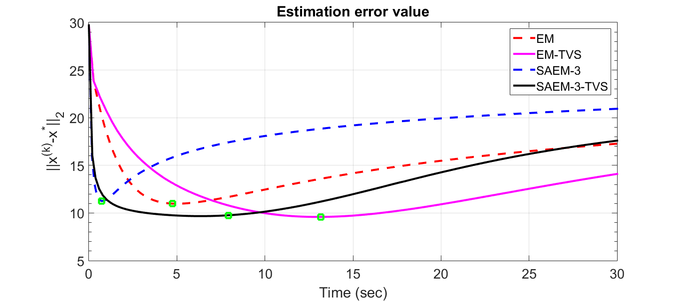
(a) Estimation Error $\|\boldsymbol{x}^{(k)}-\boldsymbol{x}^{*}\|$

(b) Total Variation vs Kullback-Leibler Curve

Figure 2: Comparison between EM and SAEM with and without superiorization.

(a) Estimation Error $||\boldsymbol{x}^{(k)}-\boldsymbol{x}^{*}\|$

(b) Total Variation vs Kullback-Leibler Curve

Figure 3: Comparison between EM and SAEM with standard superiorization and FGP superiorization.

In Figure 3 we compare the effect of the two superiorization sequences, the standard one against the proximal, produced by FGP. The plot in Figure 3(a) shows the estimation error from the current solution to the original phantom image $\boldsymbol{x}^{*}$. Now the points corresponding to images satisfying the stopping criteria are marked as red boxes. The plot in Figure 3(b) shows a curve of Kullback Leibler distance and Total Variation measurement. This plot also shows, as iteration runs, an evolution of the results moving the lower right to the upper left of Figure 3(b). Note that the final result according to the stopping criteria never reaches the upper left part, it ends in the red boxes which is the first iteration where $f(\boldsymbol{x}^{(k)})\leq 400$ .

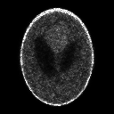
(a) EM

(b) SAEM-3

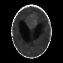
(c) EM-TVS

(d) SAEM-3-TVS

(e) EM-TVS-FGP

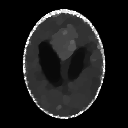
(f) SAEM-3-TVS-FGP

Figure 4: Visual Comparison between EM and SAEM images.

	em	saem-3	em-tvs	saem-3-tvs	em-tvs-fgp	saem-3-tvs-fgp
kl	$389.5\pm 21.9$	$329.5\pm 103.4$	$395.9\pm 5.7$	$398.6\pm 3.0$	$397.8\pm 4.4$	$398.1\pm 3.7$
tv	$935.2\pm 62.0$	$1076.9\pm 165.4$	$612.7\pm 50.6$	$670.9\pm 54.1$	$592.1\pm 49.7$	$653.0\pm 54.1$
mse	$10.6\pm 0.5$	$11.0\pm 0.6$	$9.2\pm 0.6$	$9.4\pm 0.7$	$9.2\pm 0.6$	$9.4\pm 0.8$
ssim	$0.72\pm 0.01$	$0.71\pm 0.01$	$0.85\pm 0.01$	$0.85\pm 0.01$	$0.85\pm 0.01$	$0.86\pm 0.01$
iter.	$21.2\pm 1.3$	$4.8\pm 1.2$	$47.1\pm 4.5$	$24.5\pm 9.0$	$46.0\pm 5.8$	$30.2\pm 6.3$
time	$2.9\pm 0.2$s	$0.4\pm 0.2$s	$8.8\pm 0.9$s	$4.6\pm 1.7$s	$7.1\pm 0.9$s	$3.8\pm 0.9$s

Table 1: Statistical indicators at the point where the stopping criterion was reached (only for ssim higher is better). The algorithms were repeated 15 times with different noise. The values shown are the sample means with 99% confidence interval.

4.2 ssaem

Now, the problem is to reconstruct images from transmission data. Therefore, the maximum likelihood model is

$$\begin{split}\min&\quad\sum_{i=1}^{m}\left\{\beta_{i}e^{-(R\boldsymbol{x})_{i}}-\alpha_{i}\log\left(e^{-(R\boldsymbol{x})_{i}}+\rho_{i}\right)\right\}\\ \operatorname{s.t.:}&\quad\boldsymbol{x}\in\mathbb{R}_{+}^{n}.\end{split}$$

In this case, we split the data in $s$ subsets (following the same construction rules than the strings) $S_{l}$, $l\in\{1,2,\dots,s\}$, such that

$$f(\boldsymbol{x})=\sum_{l=1}^{s}F_{l}(\boldsymbol{x}),$$

where

$$F_{l}(\boldsymbol{x})=\sum_{i\in S_{l}}\left\{\beta_{i}e^{-(R\boldsymbol{x})_{i}}-\alpha_{i}\log\left(e^{-(R\boldsymbol{x})_{i}}+\rho_{i}\right)\right\}.$$

Therefore

$$\frac{\partial F_{l}}{\partial x_{j}}(\boldsymbol{x})=\sum_{i\in S_{l}}r_{ij}\beta_{i}e^{-(R\boldsymbol{x})_{i}}\left\{\frac{\alpha_{i}}{\beta_{i}e^{-(R\boldsymbol{x})_{i}}+\rho_{i}}-1\right\}.$$

Tomographic setup

Data for this set of experiments was obtained at the Imaging Beamline (imx) of the Brazilian National Synchrotron Light Source (lnls) through illumination of an apple seed by x-rays. Each radiographic image was $2048\times 2048$ pixels in size and the sample was rotated by $\pi/512$ between each of the $512$ images, thereby totaling, for each slice to be reconstructed, $512$ views times $2048$ rays of tomographic count data $\alpha_{i}$. Reconstructed images have dimensions of $2048\times 2048$ pixels.

Blank scans were measured before and after the actual tomographic measurements of the sample and then data $\beta_{i}$ was obtained by linear interpolation between these two measurements. This is necessary because because lnls is a 2${}^{\text{nd}}$ generation synchrotron that does not operate in a top-up mode, i.e., the storage ring is not injected periodically in order to maintain current constant. Therefore, flux is not constant and decrease exponentially with time. As this measurement was obtained with a short exposure time, we expect that ring current (hence flux) behaves approximately as a linear model. A 4${}^{\text{th}}$ generation synchrotron source, such as the forthcoming brazilian source, Sirius, will operate in a top-up mode with more flux, i.e., samples will be measured with a short exposure time.

It is important to note that iterative methods such as those presented in this paper are extremely attractive for ultra-fast tomographic experiments, with an ultra-short exposure time and a considerable amount of noise. This is the case of soft-tissue samples where low dose should be considered and a analytical reconstruction method like filtered backprojection [11] produce low quality reconstructed images with strong streak artifacts.

4.2.1 Parameter Selection

Scaling matrix

For this algorithm we have used

$$p_{j}=\sum_{i=1}^{m}r_{ij}\{\alpha_{i}-\rho_{i}\},$$

which provides a reasonable scaling in the sense that if the approximation $\alpha_{i}\approx\beta_{i}e^{-(R\boldsymbol{x}^{(k)})_{i}}+\rho_{i}$ holds, then iterations of the form $\boldsymbol{x}^{(k+1)}=\boldsymbol{x}^{(k)}-D(\boldsymbol{x}^{(k)})\nabla f(\boldsymbol{x}^{(k)})$ become close to a multiplicative method similar to the em for emission tomography, and thus it can be written approximately as a product of coordinates of $\boldsymbol{x}^{(k)}$ with corresponding ratios of expected by observed quantities. The lower threshold was set to be $\tau=10^{-14}$.

Subsets formation

Notation for ssaem has a different meaning, where ssaem-$s$ represents ssaem using $s$ subsets of data and always only one string. The construction of the subsets was done by including all rays in a sequence of views. This sequence of views had approximately the same size on each subset. Subset processing within the string was done selecting a different random permutation for each iteration. Because only one string was used, the experimented algorithm could be described as a less general stabilized bramla. This is because it was suitable for massive paralelization in a gpu which was neccessary given the large size of the dataset. However, if more than one gpu were to be used, one string for each of them could be a reasonable way of taking advantage of the multi-gpu setup.

Stepsize sequence

As stepsize sequence for ssaem-$s$ and its superiorized version we have used

$$\lambda_{k}=\frac{\lambda_{0,s}}{(ks+1)^{0.25}},$$

where $\lambda_{0,s}$ was the largest value such that the first iteration of ssaem-$s$ would not lead to a negative value.

Superiorization sequence

The method termed ssaem-tv-$s$ corresponds to the superiorized version of ssaem-$s$ where the superiorization was obtained by application of (11) to the result of each ssaem-$s$ iteration. In this case, $N=50$ and the sequence $\{\gamma_{k}\}$ was chosen to be

$$\gamma_{k}=\frac{\gamma_{0,s}}{(ks+1)^{0.35}}.$$

Now, $\gamma_{0,s}$ was selected so that

$$\frac{\|\boldsymbol{x}^{(1/2)}-\boldsymbol{x}^{(1)}\|}{\|\boldsymbol{x}^{(0)}-\boldsymbol{x}^{(1/2)}\|}\approx 10^{-2}$$

in the following manner. First, $\boldsymbol{x}^{(1/2)}$ is computed normally using the stepsize $\lambda_{0}$ as described above. Then, a tentative value $\tilde{\mu}_{0,s}=1$ is used in order to compute $\boldsymbol{\tilde{x}}^{(1)}$. Then we set

$$\mu_{0,s}=10^{-2}\frac{\|\boldsymbol{x}^{(0)}-\boldsymbol{x}^{(1/2)}\|}{\|\boldsymbol{x}^{(1/2)}-\boldsymbol{x}^{(1)}\|}.$$

4.2.2 Numerical results

Figure 5: Comparison of several ssaem variations and its respective superiorized versions. Top: Objective function value evolution over time. Bottom: objective function versus total variation. Legend is the same for both graphics.

Figure 6: Reconstructions of apple seed slice from synchrotron radiation transmission data. Top-row: full slice images. Bottom row: details, with overlaid isocontour and location in respective images above shown as a white square. These images are the first iterates to satisfy $L_{\textsc{tr}}(\boldsymbol{x}^{(k)})\leq-1.4596\cdot 10^{11}$.

The left side of Figure 5 shows the objective function value as a function of computation time for ssaem-$s$ and ssaem-tv-$s$ with $s\in\{2,4,8,16,32\}$. Notice that increasing the number of subsets speeds up convergence in terms of reduction of objective function value over time. Superiorization reduces this convergence speed, but the fastest methods without superiorization give rise to the fastest superiorized methods as a rule of thumb.

The graphic on the right of Figure 5 displays plots of the objective function value versus total variation for the iterates of each method. The curves make clear that the superiorized version of the algorihtms always present the better compromise between data adhesion and smoothness when compared to its respective non-superiorized version. Figure 6 shows how this property translates to better image quality in practice. The lower row of Figure 6 shows isocontours overlaid on top of details of the images, in order to show that the superiorized image is noticeably smoother, therefore potentially more useful for visualization tasks. If, on the other hand, some apparent detail seems to have been removed from the image, part of these fine details may be reconstruction artifacts but we make no claims in this direction. Notice that these results are in accordance with those obtained using saem and its superiorized versions presented before.

5 Conclusions

We have studied the possibility of superiorizing incremental algorithms for maximum likelihood tomographic image reconstruction both from the theoretical and practical point of view. Several options for the superiorization were evaluated, all of which showed promising results. Furthermore, two maximum likelihood algorithms were studied, namely saem [7] and the newly introduced ssaem.

Provided numerical evidence indicates that the extra computational burden posed by the superiorization approach is justifiable given the observed improvement in image quality. Furthermore, the new algorithm ssaem was shown to have better convergent properties than saem and related methods while retaining its good practical characteristics.

References

- Beck and Teboulle [2009] Amir Beck and Marc Teboulle. Fast gradient-based algorithms for constrained total variation image denoising and deblurring problems. IEEE Transactions on Image Processing, 18(11):2419–2434, 2009. doi:10.1109/TIP.2009.2028250.
- Browne and De Pierro [1996] Jolyon Browne and Álvaro R. De Pierro. A row-action alternative to the EM algorithm for maximizing likelihoods in emission tomography. IEEE Transactions on Medical Imaging, 15(5):687–699, 1996. doi:10.1109/42.538946.
- Chambolle [2004] Antonin Chambolle. An algorithm for total variation minimization and applications. Journal of Mathematical Imaging and Vision, 20(1/2):89–97, jan 2004. ISSN 1573-7683. doi:10.1023/B:JMIV.0000011325.36760.1e.
- De Pierro and Yamagishi [2001] Álvaro R. De Pierro and Michel E. B. Yamagishi. Fast EM-like methods for maximum “a posteriori” estimates in emission tomography. IEEE Transactions on Medical Imaging, 20(4):280–288, 2001. doi:10.1109/42.921477.
- Garduño and Herman [2014] Edgar Garduño and Gabor T. Herman. Superiorization of the ML-EM algorithm. IEEE Transactions on Nuclear Science, 61(1):162–172, 2014. ISSN 00189499. doi:10.1109/TNS.2013.2283529.
- Hansen [1992] Per C. Hansen. Analysis of discrete ill-posed problems by means of the L-curve. SIAM Review, 34(4):561–580, 1992. doi:10.1137/1034115.
- Helou et al. [2014] Elias S. Helou, Yair Censor, Tai-Been Chen, I-Liang Chern, Álvaro R. De Pierro, Ming Jiang and Henry H.-S. Lu. String-averaging expectation-maximization for maximum likelihood estimation in emission tomography. Inverse Problems, 30(5):055003, 2014. doi:10.1088/0266-5611/30/5/055003.
- Helou N. and De Pierro [2005] Elias S. Helou N. and Álvaro R. De Pierro. Convergence results for scaled gradient algorithms in positron emission tomography. Inverse Problems, 21(6):1905–1914, 2005. doi:10.1088/0266-5611/21/6/007.
- Hiriart-Urruty and Lemaréchal [1993] Jean-Baptiste Hiriart-Urruty and Claude Lemaréchal. Convex Analysis and Minimization Algorithms. A Series of Comprehensive Studies in Mathematics. Springer-Verlag, Berlin, 1993.
- Hudson and Larkin [1994] H. Malcolm Hudson and Richard S. Larkin. Accelerated image reconstruction using ordered subsets of projection data. IEEE Transactions on Medical Imaging, 13(4):601–609, 1994. doi:10.1109/42.363108.
- Natterer [1986] Frank Natterer. The Mathematics of Computerized Tomography. Wiley, 1986.
- Rashed and Kudo [2013] Essam A. Rashed and Hiroyuki Kudo. Towards high-resolution synchrotron radiation imaging with statistical iterative reconstruction. Journal of Synchrotron Radiation, 20(1):116–124, 2013. doi:10.1107/S0909049512041301.
- Shepp and Vardi [1982] Larry A. Shepp and Y. Vardi. Maximum likelihood reconstruction for emission tomography. IEEE Transactions on Medical Imaging, 1(2):113–122, 1982. doi:10.1109/TMI.1982.4307558.
- Tanaka and Kudo [2003] Eiichi Tanaka and Hiroyuki Kudo. Subset-dependent relaxation in block-iterative algorithms for image reconstruction in emission tomography. Physics in Medicine and Biology, 48(10):1405–1422, 2003. doi:10.1088/0031-9155/48/10/312.
- Vardi et al. [1985] Y. Vardi, Larry A. Shepp and Linda Kaufman. A statistical model for positron emission tomography. Journal of the American Statistical Association, 80(389):8–20, 1985. doi:10.2307/2288030.
- Wang et al. [2004] Zhou Wang, Alan C. Bovik, Hamid R. Sheikh and Eero P. Simoncelli. Image quality assessment: From error visibility to structural similarity. IEEE Transactions on Image Processing, 13(4):600–612, 2004. doi:10.1109/TIP.2003.819861.