Abstract

We introduce the AdS/CFT correspondence as a natural extension of QFT in a fixed AdS background. We start by reviewing some general concepts of CFT, including the embedding space formalism. We then consider QFT in a fixed AdS background and show that one can define boundary operators that enjoy very similar properties as in a CFT, except for the lack of a stress tensor. Including a dynamical metric in AdS generates a boundary stress tensor and completes the CFT axioms. We also discuss some applications of the bulk geometric intuition to strongly coupled QFT. Finally, we end with a review of the main properties of Mellin amplitudes for CFT correlation functions and their uses in the context of AdS/CFT.

[off]

Chapter 0 TASI Lectures on AdS/CFT

[mult]26

Contents

1. 0 TASI Lectures on AdS/CFT
   1. 1 Introduction
   2. 2 Conformal Field Theory
      1. 1 Conformal Transformations
      2. 2 Local Operators
      3. 3 Ward identities
      4. 4 State-Operator Map
      5. 5 Operator Product Expansion
      6. 6 Conformal Bootstrap
      7. 7 Embedding Space Formalism
      8. 8 Large N Factorization
   3. 3 Anti-de Sitter Spacetime
      1. 1 Particle dynamics in AdS
      2. 2 Quantum Field Theory in AdS
      3. 3 Gravity with AdS boundary conditions
   4. 4 The AdS/CFT Correspondence
      1. 1 Quantum Gravity as CFT
      2. 2 String Theory
      3. 3 Finite Temperature
      4. 4 Applications
   5. 5 Mellin amplitudes
      1. 1 Definition
      2. 2 OPE $\Rightarrow$ Factorization
      3. 3 Holographic CFTs
      4. 4 Open questions

1 Introduction

The AdS/CFT correspondence [1, 2, 3] is a well established general approach to quantum gravity. However, it is often perceived as a particular construction specific to string theory. In these lectures I will argue that the AdS/CFT correspondence is the most conservative approach to quantum gravity. The quick argument goes as follows:

• System in a box - we work with Anti-de Sitter (AdS) boundary conditions because AdS is the most symmetric box with a boundary. This is useful to control large IR effects, even without dynamical gravity.

• QFT in the box - Quantum Field Theory (no gravity) in a fixed AdS background leads to the construction of boundary operators that enjoy an associative and convergent Operator Product Expansion (OPE). The AdS isometries act on the boundary operators like the conformal group in one lower dimension.

• Boundary stress-tensor from gravitons - perturbative metric fluctuations around AdS lead to a boundary stress tensor (weakly coupled to the other boundary operators).

Starting from these 3 facts it is entirely natural to define quantum gravity with AdS boundary conditions as Conformal Field Theory (CFT) in one lower dimension. Of course not all CFTs look like gravity in our universe. That requires the size of the box to be much larger than the Planck length and all higher spin particles to be very heavy (relative to the size of the box). As we shall see, these physical requirements imply that the CFT is strongly coupled and therefore hard to find or construct. The major role of string theory is to provide explicit examples of such CFTs like maximally supersymmetric Yang-Mills (SYM) theory.

There are many benefits that follow from accepting the AdS/CFT perspective. Firstly, it makes the holographic nature of gravity manifest. For example, one can immediately match the scaling of the CFT entropy density with the Bekenstein-Hawking entropy of (large) black holes in AdS. Notice that this is a consequence because it was not used as an argument for AdS/CFT in the previous paragraph. More generally, the AdS/CFT perspective let us translate questions about quantum gravity into mathematically well posed questions about CFT. Another benefit of the gauge/gravity duality is that it gives us a geometric description of QFT phenomena, which can be very useful to gain physical intuition and to create phenomenological models.

This introduction to AdS/CFT will not follow the historical order of scientific developments. Section 2 reviews general concepts in CFT. This part is not entirely self contained because this topic is discussed in detail in the chapter Conformal Bootstrap by David Simmons-Duffin [5]. The main purpose of this section is to set up notation, introduce the embedding space formalism and discuss large $N$ factorization. Section 3 deals with Anti-de Sitter (AdS) spacetime. The first goal here is to gain intuition about particle dynamics in AdS and QFT in a fixed AdS background. From this point-of-view, we will see that a gravitational theory with AdS boundary conditions naturally defines a CFT living on its boundary. In section 4, we discuss the AdS/CFT correspondence in more detail and emphasize its importance for quantum gravity. We also consider what kind of CFTs have simple AdS duals and the role of string theory. Furthermore, we discuss several applications of the gauge/gravity duality as a tool to geometrize QFT effects. Finally, in section 5, we introduce the Mellin representation of CFT correlation functions. We explain the analytic properties of Mellin amplitudes and their particular simplicity in the case of holographic CFTs.

There are many reviews of AdS/CFT available in the literature. Most of them are complementary to these lecture notes because they discuss in greater detail concrete examples of AdS/CFT realized in string theory. I leave here an incomplete list [8, 9, 10, 11, 12, 13, 14, 15, 16] that can be useful to the readers interested in knowing more about AdS/CFT. The lecture notes [17] by Jared Kaplan discuss in greater detail many of the ideas presented here.

2 Conformal Field Theory

This section briefly describes the basic concepts necessary to formulate a non-perturbative definition of CFT. In the last part, we explain in more detail the embedding space formalism for CFT and ’t Hooft’s large $N$ expansion, which will be very important in the following sections.

1 Conformal Transformations

For simplicity, in most formulas, we will consider Euclidean signature. We start by discussing conformal transformations of $\mathbb{R}^{d}$ in Cartesian coordinates,

$$ds^{2}=\delta_{\mu\nu}dx^{\mu}dx^{\nu}\ .$$ (1)

A conformal transformation is a coordinate transformation that preserves the form of the metric tensor up to a scale factor,

$$\delta_{\mu\nu}\frac{d\tilde{x}^{\mu}}{dx^{\alpha}}\frac{d\tilde{x}^{\nu}}{dx^{\beta}}=\Omega^{2}(x)\delta_{\alpha\beta}\ .$$ (2)

In other words, a conformal transformation is a local dilatation.

Exercise 2.1

Show that, for $d>2$, the most general infinitesimal conformal transformation is given by $\tilde{x}^{\mu}=x^{\mu}+\epsilon^{\mu}(x)$ with

$$\epsilon^{\mu}(x)=a^{\mu}+\lambda x^{\mu}+m^{\mu\nu}x_{\nu}+x^{2}b^{\mu}-2x^{\alpha}b_{\alpha}x^{\mu}\ .$$ (3)

In spacetime dimension $d>2$, conformal transformations form the group $SO(d+1,1)$. The generators $P_{\mu}$ and $M_{\mu\nu}$ correspond to translation and rotations and they are present in any relativistic invariant QFT. In addition, we have the generators of dilatations $D$ and special conformal transformations $K_{\mu}$. It is convenient to think of the special conformal transformations as the composition of an inversion followed by a translation followed by another inversion. Inversion is the conformal transformation

$$x^{\mu}\to\frac{x^{\mu}}{x^{2}}\ .$$ (4)

Exercise 2.2

Verify that inversion is a conformal transformation.

The form of the generators of the conformal algebra acting on functions can be obtained from

$$\phi\left(x^{\mu}+\epsilon^{\mu}(x)\right)=\left[1+i\,a^{\mu}P_{\mu}-\lambda D+\frac{i}{2}m^{\mu\nu}M_{\mu\nu}+i\,b^{\mu}K_{\mu}\right]\phi\left(x^{\mu}\right)\ ,$$ (5)

which leads to

$$P_{\mu} =-i\partial_{\mu}\ ,\qquad D =-x^{\mu}\partial_{\mu}\ ,$$ (6)

$$M_{\mu\nu} =-i\left(x_{\mu}\partial_{\nu}-x_{\nu}\partial_{\mu}\right)\ ,\qquad K_{\mu} =2ix_{\mu}x^{\nu}\partial_{\nu}-i\,x^{2}\partial_{\mu}\ .$$ (7)

Exercise 2.3

Show that the generators obey the following commutation relations

$$\left[D,P_{\mu}\right] =P_{\mu}\ ,\qquad\left[D,K_{\mu}\right]=-K_{\mu}\ ,\qquad\left[K_{\mu},P_{\nu}\right]=2\delta_{\mu\nu}D-2i\,M_{\mu\nu}\ ,$$

$$\left[M_{\mu\nu},P_{\alpha}\right] =i\left(\delta_{\mu\alpha}P_{\nu}-\delta_{\nu\alpha}P_{\mu}\right)\ ,\qquad\left[M_{\mu\nu},K_{\alpha}\right]=i\left(\delta_{\mu\alpha}K_{\nu}-\delta_{\nu\alpha}K_{\mu}\right)\ ,$$

$$\left[M_{\alpha\beta},M_{\mu\nu}\right] =i\left(\delta_{\alpha\mu}M_{\beta\nu}+\delta_{\beta\nu}M_{\alpha\mu}-\delta_{\beta\mu}M_{\alpha\nu}-\delta_{\alpha\nu}M_{\beta\mu}\right)\ .$$ (8)

2 Local Operators

Local operators are divided into two types: primary and descendant. Descendant operators are operators that can be written as (linear combinations of) derivatives of other local operators. Primary operators can not be written as derivatives of other local operators. Primary operators at the origin are annihilated by the generators of special conformal transformations. Moreover, they are eigenvectors of the dilatation generator and form irreducible representations of the rotation group $SO(d)$,

$$\left[K_{\mu},\mathcal{O}(0)\right]=0\ ,\ \ \ \ \left[D,\mathcal{O}(0)\right]=\Delta\,\mathcal{O}(0)\ ,\ \ \ \ \left[M_{\mu\nu},\mathcal{O}_{A}(0)\right]=\left[M_{\mu\nu}\right]_{A}^{B}\mathcal{O}_{B}(0)\ .$$

Correlation functions of scalar primary operators obey

$$\left\langle\mathcal{O}_{1}(\tilde{x}_{1})\dots\mathcal{O}_{n}(\tilde{x}_{n})\right\rangle=\left|\frac{\partial\tilde{x}}{\partial x}\right|_{x_{1}}^{-\frac{\Delta_{1}}{d}}\dots\left|\frac{\partial\tilde{x}}{\partial x}\right|_{x_{n}}^{-\frac{\Delta_{n}}{d}}\left\langle\mathcal{O}_{1}(x_{1})\dots\mathcal{O}_{n}(x_{n})\right\rangle$$ (9)

for all conformal transformations $x\to\tilde{x}$. As explained above, it is sufficient to impose Poincaré invariance and this transformation rule under inversion,

$$\left\langle\mathcal{O}_{1}\left(\frac{x_{1}}{x_{1}^{2}}\right)\dots\mathcal{O}_{n}\left(\frac{x_{n}}{x_{n}^{2}}\right)\right\rangle=\left(x_{1}^{2}\right)^{\Delta_{1}}\dots\left(x_{n}^{2}\right)^{\Delta_{n}}\left\langle\mathcal{O}_{1}(x_{1})\dots\mathcal{O}_{n}(x_{n})\right\rangle\ .$$

This implies that vacuum one-point functions $\left\langle\mathcal{O}(x)\right\rangle$ vanish except for the identity operator (which is the unique operator with $\Delta=0$). It also fixes the form of the two and three point functions,

$$\left\langle\mathcal{O}_{i}(x)\mathcal{O}_{j}(y)\right\rangle =\frac{\delta_{ij}}{\left(x-y\right)^{2\Delta_{i}}}\ ,$$ (10)

$$\left\langle\mathcal{O}_{1}(x_{1})\mathcal{O}_{2}(x_{2})\mathcal{O}_{3}(x_{3})\right\rangle =\frac{C_{123}}{\left|x_{12}\right|^{\Delta_{1}+\Delta_{2}-\Delta_{3}}\left|x_{13}\right|^{\Delta_{1}+\Delta_{3}-\Delta_{2}}\left|x_{23}\right|^{\Delta_{2}+\Delta_{3}-\Delta_{1}}}\ ,$$

where we have normalized the operators to have unit two point function.

The four-point function is not fixed by conformal symmetry because with four points one can construct two independent conformal invariant cross-ratios

$$u=z\bar{z}=\frac{x_{12}^{2}x_{34}^{2}}{x_{13}^{2}x_{24}^{2}}\ ,\qquad v=(1-z)(1-\bar{z})=\frac{x_{14}^{2}x_{23}^{2}}{x_{13}^{2}x_{24}^{2}}\ .$$ (11)

The general form of the four point function is

$$\left\langle\mathcal{O}(x_{1})\dots\mathcal{O}(x_{4})\right\rangle=\frac{\mathcal{A}(u,v)}{\left(x_{13}^{2}x_{24}^{2}\right)^{\Delta}}\ .$$ (12)

3 Ward identities

To define the stress-energy tensor it is convenient to consider the theory in a general background metric $g_{\mu\nu}$. Formally, we can write

$$\left\langle\mathcal{O}_{1}(x_{1})\dots\mathcal{O}_{n}(x_{n})\right\rangle_{g}=\frac{1}{Z[g]}\int[d\phi]e^{-S[\phi,g]}\mathcal{O}_{1}(x_{1})\dots\mathcal{O}_{n}(x_{n})\ ,$$ (13)

where $Z[g]=\int[d\phi]e^{-S[\phi,g]}$ is the partition function for the background metric $g_{\mu\nu}$. Recalling the classical definition

$$T^{\mu\nu}(x)=-\frac{2}{\sqrt{g}}\frac{\delta S}{\delta g_{\mu\nu}(x)}\ ,$$ (14)

it is natural to define the quantum stress-energy tensor operator via the equation

$$\frac{Z[g+\delta g]}{Z[g]}=1+\frac{1}{2}\int dx\sqrt{g}\delta g_{\mu\nu}(x)\left\langle T^{\mu\nu}(x)\right\rangle_{g}+O(\delta g^{2})\ ,$$ (15)

and

$$\left\langle\mathcal{O}_{1}(x_{1})\dots\mathcal{O}_{n}(x_{n})\right\rangle_{g+\delta g}-\left\langle\mathcal{O}_{1}(x_{1})\dots\mathcal{O}_{n}(x_{n})\right\rangle_{g}$$

$$= \frac{1}{2}\int dx\sqrt{g}\delta g_{\mu\nu}(x)\left[\left\langle T^{\mu\nu}(x)\mathcal{O}_{1}(x_{1})\dots\mathcal{O}_{n}(x_{n})\right\rangle_{g}\right.$$ (16)

$$\qquad\qquad\qquad\qquad\left.-\left\langle T^{\mu\nu}(x)\right\rangle_{g}\left\langle\mathcal{O}_{1}(x_{1})\dots\mathcal{O}_{n}(x_{n})\right\rangle_{g}\right]+O(\delta g^{2})\ .$$

Under an infinitesimal coordinate transformation $\tilde{x}^{\mu}=x^{\mu}+\epsilon^{\mu}(x)$, the metric tensor changes $\tilde{g}_{\mu\nu}=g_{\mu\nu}-\nabla_{\mu}\epsilon_{\nu}-\nabla_{\nu}\epsilon_{\mu}$ but the physics should remain invariant. In particular, the partition function $Z[g]=Z[\tilde{g}]$ and the correlation functions

$$\left\langle\mathcal{O}_{1}(\tilde{x}_{1})\dots\mathcal{O}_{n}(\tilde{x}_{n})\right\rangle_{\tilde{g}}=\left\langle\mathcal{O}_{1}(x_{1})\dots\mathcal{O}_{n}(x_{n})\right\rangle_{g}\ ,$$ (17)

do not change. This leads to the conservation equation $\left\langle\nabla_{\mu}T^{\mu\nu}(x)\right\rangle_{g}$ and

$$\sum_{i=1}^{n}\epsilon^{\mu}(x_{i})\frac{\partial}{\partial x_{i}^{\mu}}\left\langle\mathcal{O}_{1}(x_{1})\dots\mathcal{O}_{n}(x_{n})\right\rangle_{g}$$ (18)

$$=-\int dx\sqrt{g}\epsilon_{\nu}(x)\left\langle\nabla_{\mu}T^{\mu\nu}(x)\mathcal{O}_{1}(x_{1})\dots\mathcal{O}_{n}(x_{n})\right\rangle_{g}$$

for all $\epsilon^{\mu}(x)$ that decays sufficiently fast at infinity. Thus $\nabla_{\mu}T^{\mu\nu}=0$ up to contact terms.

Correlation functions of primary operators transform homogeneously under Weyl transformations of the metric

$$\left\langle\mathcal{O}_{1}(x_{1})\dots\mathcal{O}_{n}(x_{n})\right\rangle_{\Omega^{2}g}=\frac{\left\langle\mathcal{O}_{1}(x_{1})\dots\mathcal{O}_{n}(x_{n})\right\rangle_{g}}{\left[\Omega(x_{1})\right]^{\Delta_{1}}\dots\left[\Omega(x_{n})\right]^{\Delta_{n}}}\ .$$ (19)

Exercise 2.4

Show that this transformation rule under local rescalings of the metric (together with coordinate invariance) implies (9) under conformal transformations.

Consider now an infinitesimal Weyl transformation $\Omega=1+\omega$, which corresponds to a metric variation $\delta g_{\mu\nu}=2\omega g_{\mu\nu}$. From (16) and (19) we conclude that

$$\sum_{i=1}^{n}\Delta_{i}\,\omega(x_{i})\left\langle\mathcal{O}_{1}(x_{1})\dots\mathcal{O}_{n}(x_{n})\right\rangle_{g}$$

$$= -\int dx\sqrt{g}\,\omega(x)g_{\mu\nu}\left[\left\langle T^{\mu\nu}(x)\mathcal{O}_{1}(x_{1})\dots\mathcal{O}_{n}(x_{n})\right\rangle_{g}\right.$$ (20)

$$\qquad\qquad\qquad\qquad\left.-\left\langle T^{\mu\nu}(x)\right\rangle_{g}\left\langle\mathcal{O}_{1}(x_{1})\dots\mathcal{O}_{n}(x_{n})\right\rangle_{g}\right]\ .$$

Consider the following codimension 1 integral over the boundary of a region $B,$

$$I$$

$$\qquad\qquad\qquad\qquad\left.-\left\langle T^{\mu\nu}(x)\right\rangle_{g}\left\langle\mathcal{O}_{1}(x_{1})\dots\mathcal{O}_{n}(x_{n})\right\rangle_{g}\right]\ .$$

One can think of this as the total flux of the current $\epsilon_{\nu}T^{\mu\nu}$, where $\epsilon_{\nu}(x)$ is an infinitesimal conformal transformation. Gauss law tells us that this flux should be equal to the integral of the divergence of the current

$$\nabla_{\mu}\left(\epsilon_{\nu}T^{\mu\nu}\right)=\epsilon_{\nu}\nabla_{\mu}T^{\mu\nu}+\nabla_{\mu}\epsilon_{\nu}T^{\mu\nu}=\epsilon_{\nu}\nabla_{\mu}T^{\mu\nu}+\frac{1}{d}\nabla_{\alpha}\epsilon^{\alpha}g_{\mu\nu}T^{\mu\nu}\ ,$$ (21)

where we used the symmetry of the stress-energy tensor $T^{\mu\nu}=T^{\nu\mu}$ and the definition of an infinitesimal conformal transformation $\nabla_{\mu}\epsilon_{\nu}+\nabla_{\nu}\epsilon_{\mu}=\frac{2}{d}\nabla_{\alpha}\epsilon^{\alpha}g_{\mu\nu}$. Using Gauss law and (18) and (20) we conclude that

$$I=-\sum_{x_{i}\in B}\left[\epsilon^{\mu}(x_{i})\frac{\partial}{\partial x_{i}^{\mu}}+\frac{\Delta_{i}}{d}\nabla_{\alpha}\epsilon^{\alpha}(x_{i})\right]\left\langle\mathcal{O}_{1}(x_{1})\dots\mathcal{O}_{n}(x_{n})\right\rangle_{g}\ .$$ (22)

The equality of (LABEL:eq:WardIdentityFlux) and (22) for any infinitesimal conformal transformation (3) is the most useful form of the conformal Ward identities.

Exercise 2.5

Conformal symmetry fixes the three-point function of a spin 2 primary operator and two scalars up to an overall constant,

$$\langle\mathcal{O}(x_{1})\mathcal{O}(x_{2})T^{\mu\nu}(x_{3})\rangle=C_{12T}\frac{H^{\mu\nu}(x_{1},x_{2},x_{3})}{|x_{12}|^{2\Delta-d+2}|x_{13}|^{d-2}|x_{23}|^{d-2}}\ ,$$ (23)

where

$$H^{\mu\nu}=V^{\mu}V^{\nu}-\frac{1}{d}V_{\alpha}V^{\alpha}\delta^{\mu\nu}\ ,\qquad V^{\mu}=\frac{x_{13}^{\mu}}{x_{13}^{2}}-\frac{x_{23}^{\mu}}{x_{23}^{2}}\ .$$ (24)

Write the conformal Ward identity (LABEL:eq:WardIdentityFlux)=(22) for the three point function $\langle T^{\mu\nu}(x)\mathcal{O}(0)\mathcal{O}(y)\rangle$ for the case of an infinitesimal dilation $\epsilon^{\mu}(x)=\lambda x^{\mu}$ and with the surface $\partial B$ being a sphere centred at the origin and with radius smaller than $|y|$. Use this form of the conformal Ward identity in the limit of an infinitesimally small sphere $\partial B$ and formula (23) for the three point function to derive

$$C_{\mathcal{OO}T}=-\frac{d\Delta}{d-1}\frac{1}{S_{d}}\ ,$$ (25)

where $S_{d}=\frac{2\pi^{d/2}}{\Gamma(d/2)}$ is the volume of a $(d-1)$-dimensional unit sphere.

4 State-Operator Map

Consider $\mathbb{R}^{d}$ in spherical coordinates. Writing the radial coordinate as $r=e^{\tau}$ we find

$$ds^{2}=dr^{2}+r^{2}d\Omega_{d-1}^{2}=e^{2\tau}\left(d\tau^{2}+d\Omega_{d-1}^{2}\right)\ .$$ (26)

Thus, the cylinder $\mathbb{R}\times S^{d-1}$ can be obtained as a Weyl transformation of euclidean space $\mathbb{R}^{d}$.

Exercise 2.6

Compute the two-point function of a scalar primary operator on the cylinder using the Weyl transformation property (19).

A local operator inserted at the origin of $\mathbb{R}^{d}$ prepares a state at $\tau=-\infty$ on the cylinder. On the other hand, a state on a constant time slice of the cylinder can be propagated backwards in time until it corresponds to a boundary condition on a arbitrarily small sphere around the origin of $\mathbb{R}^{d}$, which defines a local operator. Furthermore, time translations on the cylinder correspond to dilatations on $\mathbb{R}^{d}$. This teaches us that the spectrum of the dilatation generator on $\mathbb{R}^{d}$ is the same as the energy spectrum for the theory on $\mathbb{R}\times S^{d-1}$.

5 Operator Product Expansion

The Operator Product Expansion (OPE) between two scalar primary operators takes the following form

$$\mathcal{O}_{i}(x)\mathcal{O}_{j}(0)=\sum_{k}C_{ijk}|x|^{\Delta_{k}-\Delta_{i}-\Delta_{j}}\left[\mathcal{O}_{k}(0)+\underbrace{\beta\,x^{\mu}\partial_{\mu}\mathcal{O}_{k}(0)+\dots}_{{\rm descendants}}\right]$$ (27)

where $\beta$ denotes a number determined by conformal symmetry. For simplicity we show only the contribution of a scalar operator $\mathcal{O}_{k}$. In general, in the OPE of two scalars there are primary operators of all spins.

Exercise 2.7

Compute $\beta$ by using this OPE inside a three-point function.

The OPE has a finite radius of convergence inside correlation functions. This follows from the state operator map with an appropriate choice of origin for radial quantization.

6 Conformal Bootstrap

Using the OPE successively one can reduce any $n-$point function to a sum of one-point functions, which all vanish except for the identity operator. Thus, knowing the operator content of the theory, i.e. the scaling dimensions $\Delta$ and $SO(d)$ irreps $\mathcal{R}$ of all primary operators, and the OPE coefficients $C_{ijk}$, one can determine all correlation functions of local operators. This set of data is called CFT data because it essentially defines the theory. The CFT data is not arbitrary, it must satisfy several constraints:

• OPE associativity - Different ways of using the OPE to compute a correlation function must give the same result. This leads to the conformal bootstrap equations described below.

• Existence of stress-energy tensor - The stress-energy tensor $T_{\mu\nu}$ is a conserved primary operator (with $\Delta=d$) whose correlation functions obey the conformal Ward identities.

• Unitarity - In our Euclidean context this corresponds to reflection positivity and it implies lower bounds on the scaling dimensions. It also implies that one can choose a basis of real operators where all OPE coefficients are real. In the context of statistical physics, there are interesting non-unitary CFTs.

It is sufficient to impose OPE associativity for all four-point functions of the theory. For a four-point function of scalar operators, the bootstrap equation reads

$$\sum_{k}C_{12k}C_{k34}G_{\Delta_{k},l_{k}}^{(12)(34)}(x_{1},\dots,x_{4})=\sum_{q}C_{13q}C_{q24}G_{\Delta_{q},l_{q}}^{(13)(24)}(x_{1},\dots,x_{4})\,,$$

where $G_{\Delta,l}$ are conformal blocks, which encode the contribution from a primary operator of dimension $\Delta$ and spin $l$ and all its descendants.

7 Embedding Space Formalism

The conformal group $SO(d+1,1)$ acts naturally on the space of light rays through the origin of $\mathbb{R}^{d+1,1}$,

$$-\left(P^{0}\right)^{2}+\left(P^{1}\right)^{2}+\dots+\left(P^{d+1}\right)^{2}=0\ .$$ (28)

A section of this light-cone is a $d-$dimensional manifold where the CFT lives. For example, it is easy to see that the Poincaré section $P^{0}+P^{d+1}=1$ is just $\mathbb{R}^{d}$. To see this parametrize this section using

$$P^{0}(x)=\frac{1+x^{2}}{2}\ ,\qquad P^{\mu}(x)=x^{\mu}\ ,\qquad P^{d+1}(x)=\frac{1-x^{2}}{2}\ ,$$ (29)

with $\mu=1,\dots,d$ and $x^{\mu}\in\mathbb{R}^{d}$ and compute the induced metric. In fact, any conformally flat manifold can be obtained as a section of the light-cone in the embedding space $\mathbb{R}^{d+1,1}$. Using the parametrization $P^{A}=\Omega(x)P^{A}(x)$ with $x^{\mu}\in\mathbb{R}^{d}$, one can easily show that the induced metric is simply given by $ds^{2}=\Omega^{2}(x)\delta_{\mu\nu}dx^{\mu}dx^{\nu}$. With this is mind, it is natural to extend a primary operator from the physical section to the full light-cone with the following homogeneity property

$$\mathcal{O}(\lambda P)=\lambda^{-\Delta}\mathcal{O}(P)\ ,\qquad\lambda\in\mathbb{R}\ .$$ (30)

This implements the Weyl transformation property (19). One can then compute correlation functions directly in the embedding space, where the constraints of conformal symmetry are just homogeneity and $SO(d+1,1)$ Lorentz invariance. Physical correlators are simply obtained by restricting to the section of the light-cone associated with the physical space of interest. This idea goes back to Dirac [18] and has been further develop by many authors [19, 20, 21, 22, 23, 24, 25].

Exercise 2.8

Rederive the form of two and three point functions of scalar primary operators in $\mathbb{R}^{d}$ using the embedding space formalism.

Vector primary operators can also be extended to the embedding space. In this case, we impose

$$P^{A}\mathcal{O}_{A}(P)=0\ ,\qquad\mathcal{O}_{A}(\lambda P)=\lambda^{-\Delta}\mathcal{O}_{A}(P)\ ,\qquad\lambda\in\mathbb{R}\ ,$$ (31)

and the physical operator is obtained by projecting the indices to the section,

$$\mathcal{O}_{\mu}(x)=\left.\frac{\partial P^{A}}{\partial x^{\mu}}\mathcal{O}_{A}(P)\right|_{P^{A}=P^{A}(x)}\ .$$ (32)

Notice that this implies a redundancy: $\mathcal{O}_{A}(P)\to\mathcal{O}_{A}(P)+P_{A}\Lambda(P)$ gives rise to the same physical operator $\mathcal{O}(x)$, for any scalar function $\Lambda(P)$ such that $\Lambda(\lambda P)=\lambda^{-\Delta-1}\Lambda(P)$. This redundancy together with the constraint $P^{A}\mathcal{O}_{A}(P)=0$ remove 2 degrees of freedom of the $(d+2)$-dimensional vector $\mathcal{O}_{A}$.

Exercise 2.9

Show that the two-point function of vector primary operators is given by

$$\left\langle\mathcal{O}^{A}(P_{1})\mathcal{O}^{B}(P_{2})\right\rangle=const\frac{\eta^{AB}\left(P_{1}\cdot P_{2}\right)-P_{2}^{A}P_{1}^{B}}{\left(-2P_{1}\cdot P_{2}\right)^{\Delta+1}}\ ,$$ (33)

up to redundant terms.

Exercise 2.10

Consider the parametrization $P^{A}=\left(P^{0},P^{\mu},P^{d+1}\right)=\left(\cosh\tau,\Omega^{\mu},-\sinh\tau\right)$ of the global section $\left(P^{0}\right)^{2}-\left(P^{d+1}\right)^{2}=1$, where $\Omega^{\mu}$ ($\mu=1,\dots,d$) parametrizes a unit $(d-1)-$dimensional sphere, $\Omega\cdot\Omega=1$. Show that this section has the geometry of a cylinder exactly like the one used for the state-operator map.

Conformal correlation functions extended to the light-cone of $\mathbb{R}^{1,d+1}$ are annihilated by the generators of $SO(1,d+1)$

$$\sum_{i=1}^{n}J_{AB}^{(i)}\left\langle\mathcal{O}_{1}(P_{1})\dots\mathcal{O}_{n}(P_{n})\right\rangle=0\ ,$$ (34)

where $J_{AB}^{(i)}$ is the generator

$$J_{AB}=-i\left(P_{A}\frac{\partial}{\partial P^{B}}-P_{B}\frac{\partial}{\partial P^{A}}\right)\ ,$$ (35)

acting on the point $P_{i}$. For a given choice of light cone section, some generators will preserve the section and some will not. The first are Killing vectors (isometry generators) and the second are conformal Killing vectors. The commutation relations give the usual Lorentz algebra

$$\left[J_{AB},J_{CD}\right]=i\left(\eta_{AC}J_{BD}+\eta_{BD}J_{AC}-\eta_{BC}J_{AD}-\eta_{AD}J_{BC}\right)\ .$$ (36)

Exercise 2.11

Check that the conformal algebra (8) follows from (36) and

$$D =-i\,J_{0,d+1}\ ,\qquad P_{\mu} =J_{\mu 0}-J_{\mu,d+1}\ ,$$

$$M_{\mu\nu} =J_{\mu\nu}\ , K_{\mu} =J_{\mu 0}+J_{\mu,d+1}.$$ (37)

Exercise 2.12

Show that equation (34) for $J_{AB}=J_{0,d+1}$ implies time translation invariance on the cylinder

$$\sum_{i=1}^{n}\frac{\partial}{\partial\tau_{i}}\left\langle\mathcal{O}_{1}(\tau_{1},\Omega_{1})\dots\mathcal{O}_{n}(\tau_{n},\Omega_{n})\right\rangle=0\ ,$$ (38)

and dilatation invariance on $\mathbb{R}^{d}$

$$\sum_{i=1}^{n}\left(\Delta_{i}+x_{i}^{\mu}\frac{\partial}{\partial x_{i}^{\mu}}\right)\left\langle\mathcal{O}_{1}(x_{1})\dots\mathcal{O}_{n}(x_{n})\right\rangle=0\ .$$ (39)

In this case, you will need to use the differential form of the homogeneity property $P^{A}\frac{\partial}{\partial P^{A}}\mathcal{O}_{i}(P)=-\Delta_{i}\mathcal{O}_{i}(P)$. It is instructive to do this exercise for the other generators as well.

8 Large N Factorization

Consider a $U(N)$ gauge theory with fields valued in the adjoint representation. Schematically, we can write the action as

$$S=\frac{N}{\lambda}\int dx\ {\rm Tr}\left[\left(D\Phi\right)^{2}+c_{3}\Phi^{3}+c_{4}\Phi^{4}+\dots\right]$$ (40)

where we introduced the ’t Hooft coupling $\lambda=g_{YM}^{2}N$ and $c_{i}$ are other coupling constants independent of $N$. Following ’t Hooft [26], we consider the limit of large $N$ with $\lambda$ kept fixed. The propagator of an adjoint field obeys

$$\left\langle\Phi_{j}^{i}\Phi_{l}^{k}\right\rangle\propto\frac{\lambda}{N}\delta_{l}^{i}\delta_{j}^{k}$$ (41)

where we used the fact that the adjoint representation can be represented as the direct product of the fundamental and the anti-fundamental representation. This suggests that one can represent a propagator by a double line, where each line denotes the flow of a fundamental index. Start by considering the vacuum diagrams in this language. A diagram with $V$ vertices, $E$ propagators (or edges) and $F$ lines (or faces) scales as

$$\left(\frac{N}{\lambda}\right)^{V}\left(\frac{\lambda}{N}\right)^{E}N^{F}=\left(\frac{N}{\lambda}\right)^{\chi}\lambda^{F}\ ,$$ (42)

where $\chi=V+F-E=2-2g$ is the minimal Euler character of the two dimensional surface where the double line diagram can be embedded and $g$ is the number of handles of this surface. Therefore, the large $N$ limit is dominated by diagrams that can be drawn on a sphere $(g=0)$. These diagrams are called planar diagrams. For a given topology, there is an infinite number of diagrams that contribute with increasing powers of the coupling $\lambda$, corresponding to tesselating the surface with more and more faces. Figure 1 shows two examples of vacuum diagrams in the double line notation. This topological expansion has the structure of string perturbation theory with $\lambda/N$ playing the role of the string coupling. As we shall see this is precisely realized in maximally supersymmetric Yang-Mills theory (SYM).

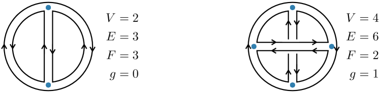
Figure 1: Vacuum diagrams in the double line notation. Interaction vertices are marked with a small blue dot. The left diagram is planar while the diagram on the right has the topology of a torus (genus 1 surface).

Let us now consider single-trace local operators of the form $\mathcal{O}=c_{J}{\rm Tr}\left(\Phi^{J}\right)$, where $c_{J}$ is a normalization constant independent of $N$. Adapting the argument above, it is easy to conclude that the connected correlators are given by a large $N$ expansion of the form

$$\left\langle\mathcal{O}_{1}\dots\mathcal{O}_{n}\right\rangle_{c}=\sum_{g=0}^{\infty}N^{2-n-2g}f_{g}(\lambda)\ ,$$ (43)

which is dominated by the planars diagrams $(g=0)$. Moreover, we see that the planar two-point function is independent of $N$ while connected higher point functions are suppressed by powers of $N$. This is large $N$ factorization. In particular it implies that the two-point function of a multi-trace operator $\tilde{\mathcal{O}}(x)=:\mathcal{O}_{1}(x)\dots\mathcal{O}_{k}(x):$ is dominated by the product of the two-point functions of its single-trace constituents

$$\left\langle\tilde{\mathcal{O}}(x)\tilde{\mathcal{O}}(y)\right\rangle\approx\prod_{i}\left\langle\mathcal{O}_{i}(x)\mathcal{O}_{i}(y)\right\rangle=\frac{1}{(x-y)^{2\sum_{i}\Delta_{i}}}\ ,$$ (44)

where we assumed that the single-trace operators were scalar conformal primaries properly normalized. We conclude that the scaling dimension of the multi-trace operator $\tilde{\mathcal{O}}$ is given by $\sum_{i}\Delta_{i}+O(1/N^{2})$ . In other words, the space of local operators in a large $N$ CFT has the structure of a Fock space with single-trace operators playing the role of single particle states of a weakly coupled theory. This is the form of large $N$ factorization relevant for AdS/CFT. However, notice that conformal invariance was not important for the argument. It is well known that large $N$ factorization also occurs in confining gauge theories. Physically, it means that colour singlets (like glueballs or mesons) interact weakly in large $N$ gauge theories (see [27] for a clear summary).

The stress tensor has a natural normalization that follows from the action, $T_{\mu\nu}\sim\frac{N}{\lambda}{\rm Tr}\left(\partial_{\mu}\Phi\partial_{\nu}\Phi\right)$. This leads to the large $N$ scaling

$$\left\langle T_{\mu_{1}\nu_{1}}(x_{1})\dots T_{\mu_{n}\nu_{n}}(x_{n})\right\rangle_{c}\sim N^{2}\ ,$$ (45)

which will be important below. This normalization of $T_{\mu\nu}$ is also fixed by the Ward identities.

3 Anti-de Sitter Spacetime

Euclidean AdS spacetime is the hyperboloid

$$-\left(X^{0}\right)^{2}+\left(X^{1}\right)^{2}+\dots+\left(X^{d+1}\right)^{2}=-R^{2}\ ,\qquad X^{0}>0\ ,$$ (46)

embedded in $\mathbb{R}^{d+1,1}$. For large values of $X^{0}$ this hyperboloid approaches the light-cone of the embedding space that we discussed in section 7. It is clear from the definition that Euclidean AdS is invariant under $SO(d+1,1)$. The generators are given by

$$J_{AB}=-i\left(X_{A}\frac{\partial}{\partial X^{B}}-X_{B}\frac{\partial}{\partial X^{A}}\right)\ .$$ (47)

Poincaré coordinates are defined by

$$X^{0} = R\frac{1+x^{2}+z^{2}}{2z}$$

$$X^{\mu} = R\frac{x^{\mu}}{z}$$ (48)

$$X^{d+1} = R\frac{1-x^{2}-z^{2}}{2z}$$

where $x^{\mu}\in\mathbb{R}^{d}$ and $z>0$. In these coordinates, the metric reads

$$ds^{2}=R^{2}\frac{dz^{2}+\delta_{\mu\nu}dx^{\mu}dx^{\nu}}{z^{2}}\ .$$ (49)

This shows that AdS is conformal to $\mathbb{R}^{+}\times\mathbb{R}^{d}$ whose boundary at $z=0$ is just $\mathbb{R}^{d}$. These coordinates make explicit the subgroup $SO(1,1)\times ISO(d)$ of the full isometry group of AdS. These correspond to dilatation and Poincaré symmetries inside the $d-$dimensional conformal group. In particular, the dilatation generator is

$$D=-i\,J_{0,d+1}=-X_{0}\frac{\partial}{\partial X^{d+1}}+X_{d+1}\frac{\partial}{\partial X^{0}}=-z\frac{\partial}{\partial z}-x^{\mu}\frac{\partial}{\partial x^{\mu}}\ .$$ (50)

Another useful coordinate system is

$$X^{0} = R\cosh\tau\cosh\rho$$

$$X^{\mu} = R\,\Omega^{\mu}\sinh\rho$$ (51)

$$X^{d+1} = -R\sinh\tau\cosh\rho$$

where $\Omega^{\mu}$ ($\mu=1,\dots,d$) parametrizes a unit $(d-1)-$dimensional sphere, $\Omega\cdot\Omega=1$. The metric is given by

$$ds^{2}=R^{2}\left[\cosh^{2}\rho\,d\tau^{2}+d\rho^{2}+\sinh^{2}\rho\,d\Omega_{d-1}^{2}\right]\ .$$ (52)

To understand the global structure of this spacetime it is convenient to change the radial coordinate via $\tanh\rho=\sin r$ so that $r\in[0,\frac{\pi}{2}[$. Then, the metric becomes

$$ds^{2}=\frac{R^{2}}{\cos^{2}r}\left[d\tau^{2}+dr^{2}+\sin^{2}r\,d\Omega_{d-1}^{2}\right]\ ,$$ (53)

which is conformal to a solid cylinder whose boundary at $r=\frac{\pi}{2}$ is $\mathbb{R}\times S^{d-1}$. In these coordinates, the dilatation generator $D=-i\,J_{0,d+1}=-\frac{\partial}{\partial\tau}$ is the hamiltonian conjugate to global time.

1 Particle dynamics in AdS

For most purposes it is more convenient to work in Euclidean signature and analytically continue to Lorentzian signature only at the end of the calculation. However, it is important to discuss the Lorentzian signature to gain some intuition about real time dynamics. In this case, AdS is defined by the universal cover of the manifold

$$-\left(X^{0}\right)^{2}+\left(X^{1}\right)^{2}+\dots+\left(X^{d}\right)^{2}-\left(X^{d+1}\right)^{2}=-R^{2}\ ,$$ (54)

embedded in $\mathbb{R}^{d,2}$. The universal cover means that we should unroll the non-contractible (timelike) cycle. To see this explicitly it is convenient to introduce global coordinates

$$X^{0} = R\cos t\cosh\rho$$

$$X^{\mu} = R\,\Omega^{\mu}\sinh\rho$$ (55)

$$X^{d+1} = -R\sin t\cosh\rho$$

where $\Omega^{\mu}$ ($\mu=1,\dots,d$) parametrizes a unit $(d-1)-$dimensional sphere. The original hyperboloid is covered with $t\in[0,2\pi[$ but we consider $t\in\mathbb{R}$. The metric is given by

$$ds^{2}=R^{2}\left[-\cosh^{2}\rho\,dt^{2}+d\rho^{2}+\sinh^{2}\rho\,d\Omega_{d-1}^{2}\right]\ .$$ (56)

To understand the global structure of this spacetime it is convenient to change the radial coordinate via $\tanh\rho=\sin r$ so that $r\in[0,\frac{\pi}{2}[$. Then, the metric becomes

$$ds^{2}=\frac{R^{2}}{\cos^{2}r}\left[-dt^{2}+dr^{2}+\sin^{2}r\,d\Omega_{d-1}^{2}\right]\ ,$$ (57)

which is conformal to a solid cylinder whose boundary at $r=\frac{\pi}{2}$ is $\mathbb{R}\times S^{d-1}$.

Geodesics are given by the intersection of AdS with 2-planes through the origin of the embedding space. In global coordinates, the simplest timelike geodesic describes a particle sitting at $\rho=0$. This corresponds to (the universal cover of) the intersection of $X^{\mu}=0$ for $\mu=1,\dots,d$ with the hyperboloid (54). Performing a boost in the $X^{1},X^{d+1}$ plane we can obtain an equivalent timelike geodesic $X^{1}\cosh\beta=X^{d+1}\sinh\beta$ and $X^{\mu}=0$ for $\mu=2,\dots,d$. In global coordinates, this gives an oscillating trajectory

$$\tanh\rho=\tanh\beta\,\sin t\ ,$$ (58)

with period $2\pi$. In fact, all timelike geodesics oscillate with period $2\pi$ in global time. One can say AdS acts like a box that confines massive particles. However, it is a very symmetric box that does not have a center because all points are equivalent.

Null geodesics in AdS are also null geodesics in the embedding space. For example, the null ray $X^{d+1}-X^{1}=X^{0}-R=X^{\mu}=0$ for $\mu=2,\dots,d$ is a null ray in AdS which in global coordinates is given by $\cosh\rho=\frac{1}{\cos t}$. This describes a light ray that passes through the origin at $t=0$ and reaches the conformal boundary $\rho=\infty$ at $t=\pm\frac{\pi}{2}$. All light rays in AdS start and end at the conformal boundary traveling for a global time interval equal to $\pi$.

One can also introduce Poincaré coordinates

$$X^{\mu} = R\frac{x^{\mu}}{z}$$

$$X^{d} = \frac{R}{2}\frac{1-x^{2}-z^{2}}{z}$$ (59)

$$X^{d+1} = \frac{R}{2}\frac{1+x^{2}+z^{2}}{z}$$

where now $\mu=0,1,\dots,d-1$ and $x^{2}=\eta_{\mu\nu}x^{\mu}x^{\nu}$. However, in Lorentzian signature, Poincaré coordinates do not cover the entire spacetime. Surfaces of constant $z$ approach the light-like surface $X^{d}+X^{d+1}=0$ when $z\to\infty$. This null surface is often called the Poincaré horizon.

We have seen that AdS acts like a box for classical massive particles. Quantum mechanically, this confining potential gives rise to a discrete energy spectrum. Consider the Klein-Gordon equation

$$\nabla^{2}\phi=m^{2}\phi\ ,$$ (60)

in global coordinates (56). In order to emphasize the correspondence with CFT we will solve this problem using an indirect route. Firstly, consider the action of the quadratic Casimir of the AdS isometry group on a scalar field

$$\frac{1}{2}J_{AB}J^{BA}\phi=\left[-X^{2}\partial_{X}^{2}+X\cdot\partial_{X}\left(d+X\cdot\partial_{X}\right)\right]\phi\ .$$ (61)

Formally, we are extending the function $\phi$ from AdS, defined by the hypersurface $X^{2}=-R^{2}$, to the embedding space. However, the action of the quadratic Casimir is independent of this extension because the generators $J_{AB}$ are interior to AdS, i.e. $\left[J_{AB},X^{2}+R^{2}\right]=0$. If we foliate the embedding space $\mathbb{R}^{d,2}$ with AdS surfaces of different radii $R$, we obtain that the laplacian in the embedding space can be written as

$$\partial_{X}^{2}=-\frac{1}{R^{d+1}}\frac{\partial}{\partial R}R^{d+1}\frac{\partial}{\partial R}+\nabla_{AdS}^{2}\ .$$ (62)

Substituting this in (61) and noticing that $X\cdot\partial_{X}=R\partial_{R}$ we conclude that

$$\frac{1}{2}J_{AB}J^{BA}\phi=R^{2}\nabla_{AdS}^{2}\phi\ .$$ (63)

Therefore, we should identify $m^{2}R^{2}$ with the quadratic Casimir of the conformal group.

The Lorentzian version of the conformal generators (37) is

$$D =-J_{0,d+1}\ ,\qquad P_{\mu} =J_{\mu 0}+i\,J_{\mu,d+1}\ ,$$ (64)

$$M_{\mu\nu} =J_{\mu\nu}\ ,\qquad K_{\mu} =J_{\mu 0}-i\,J_{\mu,d+1}\ .$$ (65)

Exercise 3.1

Show that, in global coordinates, the conformal generators take the form

$$D =i\frac{\partial}{\partial t}\ ,\qquad M_{\mu\nu}=-i\left(\Omega_{\mu}\frac{\partial}{\partial\Omega^{\nu}}-\Omega_{\nu}\frac{\partial}{\partial\Omega^{\mu}}\right)\ ,$$

$$P_{\mu} =-ie^{-it}\left[\Omega_{\mu}\left(\partial_{\rho}-i\tanh\rho\,\partial_{t}\right)+\frac{1}{\tanh\rho}\nabla_{\mu}\right]\ ,$$

$$K_{\mu} =ie^{it}\left[\Omega_{\mu}\left(-\partial_{\rho}-i\tanh\rho\,\partial_{t}\right)-\frac{1}{\tanh\rho}\nabla_{\mu}\right]\ ,$$

where $\nabla_{\mu}=\frac{\partial}{\partial\Omega^{\mu}}-\Omega_{\mu}\Omega^{\nu}\frac{\partial}{\partial\Omega^{\nu}}$ is the covariant derivative on the unit sphere $S^{d-1}$.

In analogy with the CFT construction we can look for primary states, which are annihilated by $K_{\mu}$ and are eigenstates of the hamiltonian, $D\phi=\Delta\phi$. The condition $K_{\mu}\phi=0$ splits in one term proportional to $\Omega_{\mu}$ and one term orthogonal to $\Omega_{\mu}$. The second term implies that $\phi$ is independent of the angular variables $\Omega^{\mu}$. The first term gives $\left(\partial_{\rho}+\Delta\tanh\rho\right)\phi=0$, which implies that

$$\phi\propto\left(\frac{e^{-it}}{\cosh\rho}\right)^{\Delta}=\left(\frac{R}{X^{0}-X^{d+1}}\right)^{\Delta}\ .$$ (66)

This is the lowest energy state. One can get excited states acting with $P_{\mu}$. Notice that all this states will have the same value of the quadratic Casimir

$$\frac{1}{2}J_{AB}J^{BA}\phi=\Delta(\Delta-d)\phi\ .$$ (67)

This way one can generate all normalizable solutions of $\nabla^{2}\phi=m^{2}\phi$ with $m^{2}R^{2}=\Delta(\Delta-d)$. This shows that the one-particle energy spectrum is given by $\omega=\Delta+l+2n$ where $l=0,1,2,\dots$ is the spin, generated by acting with $P_{\mu_{1}}\dots P_{\mu_{l}}-traces\$, and $n=0,1,2,\dots$ is generated by acting with $\left(P^{2}\right)^{n}$.

Exercise 3.2

Given the symmetry of the metric (53) we can look for solutions of the form

$$\phi=e^{i\omega t}Y_{l}(\Omega)F(r)\ ,$$ (68)

where $Y_{l}(\Omega)$ is a spherical harmonic with eigenvalue $-l(l+d-2)$ of the laplacian on the unit sphere $S^{d-1}$. Derive a differential equation for $F(r)$ and show that it is solved by

$$F(r)=\left(\cos r\right)^{\Delta}\left(\sin r\right)^{l}\ _{2}F_{1}\left(\frac{l+\Delta-\omega}{2},\frac{l+\Delta+\omega}{2},l+\frac{d}{2},\sin r\right)\ ,$$ (69)

with $2\Delta=d+\sqrt{d^{2}+4(mR)^{2}}$. We chose this solution because it is smooth at $r=0$. Now we also need to impose another boundary condition at the boundary of AdS $r=\frac{\pi}{2}$. Imposing that there is no energy flux through the boundary leads to the quantization of the energies $|\omega|=\Delta+l+2n$ with $n=0,1,2,\dots$ (see reference [8]).

If there are no interactions between the particles in AdS, then the Hilbert space is a Fock space and the energy of a multi-particle state is just the sum of the energies of each particle. Turning on small interactions leads to small energy shifts of the multi-particle states. This structure is very similar to the space of local operators in large $N$ CFTs if we identify single-particle states with single-trace operators.

2 Quantum Field Theory in AdS

Let us now return to Euclidean signature and consider QFT on the AdS background. For simplicity, consider a free scalar field with action

$$S=\int_{AdS}dX\left[\frac{1}{2}\left(\nabla\phi\right)^{2}+\frac{1}{2}m^{2}\phi^{2}\right]\ .$$ (70)

The two-point function $\left\langle\phi(X)\phi(Y)\right\rangle$ is given by the propagator $\Pi(X,Y)$, which obeys

$$\left[\nabla_{X}^{2}-m^{2}\right]\Pi(X,Y)=-\delta(X,Y)\ .$$ (71)

From the symmetry of the problem it is clear that the propagator can only depend on the invariant $X\cdot Y$ or equivalently on the chordal distance $\zeta=(X-Y)^{2}/R^{2}$. From now on we will set $R=1$ and all lengths will be expressed in units of the AdS radius.

Exercise 3.3

Use (61) and (63) to show that

$$\Pi(X,Y)=\frac{\mathcal{C}_{\Delta}}{\zeta^{\Delta}}\ _{2}F_{1}\left(\Delta,\Delta-\frac{d}{2}+\frac{1}{2},2\Delta-d+1,-\frac{4}{\zeta}\right)\ ,$$ (72)

where $2\Delta=d+\sqrt{d^{2}+(2m)^{2}}$ and

$$\mathcal{C}_{\Delta}=\frac{\Gamma(\Delta)}{2\pi^{\frac{d}{2}}\Gamma\left(\Delta-\frac{d}{2}+1\right)}\ .$$ (73)

For a free field, higher point functions are simply given by Wick contractions. For example,

$$\left\langle\phi(X_{1})\phi(X_{2})\phi(X_{3})\phi(X_{4})\right\rangle =\Pi(X_{1},X_{2})\Pi(X_{3},X_{4})+\Pi(X_{1},X_{3})\Pi(X_{2},X_{4})$$

$$+\Pi(X_{1},X_{4})\Pi(X_{2},X_{3})\ .$$ (74)

Weak interactions of $\phi$ can be treated perturbatively. Suppose the action includes a cubic term,

$$S=\int_{AdS}dX\left[\frac{1}{2}\left(\nabla\phi\right)^{2}+\frac{1}{2}m^{2}\phi^{2}+\frac{1}{3!}g\phi^{3}\right]\ .$$ (75)

Then, there is a non-vanishing three-point function

$$\left\langle\phi(X_{1})\phi(X_{2})\phi(X_{3})\right\rangle=-g\int_{AdS}dY\,\Pi(X_{1},Y)\Pi(X_{2},Y)\Pi(X_{3},Y)+O(g^{3})\ ,$$

and a connected part of the four-point function of order $g^{2}$. This is very similar to perturbative QFT in flat space.

Given a correlation function in AdS we can consider the limit where we send all points to infinity. More precisely, we introduce

$$\mathcal{O}(P)=\frac{1}{\sqrt{C_{\Delta}}}\lim_{\lambda\to\infty}\lambda^{\Delta}\,\phi\left(X=\lambda P+\dots\right),$$ (76)

where $P$ is a future directed null vector in $\mathbb{R}^{d+1,1}$ and the $\dots$ denote terms that do not grow with $\lambda$ whose only purpose is to enforce the AdS condition $X^{2}=-1$. In other words, the operator $\mathcal{O}(P)$ is the limit of the field $\phi(X)$ when $X$ approaches the boundary point $P$ of AdS. Notice that, by definition, the operator $\mathcal{O}(P)$ obeys the homogeneity condition (30). Correlation functions of $\mathcal{O}$ are naturally defined by the limit of correlation functions of $\phi$ in AdS. For example, the two-point function is given by

$$\left\langle\mathcal{O}(P_{1})\mathcal{O}(P_{2})\right\rangle=\frac{1}{\left(-2P_{1}\cdot P_{2}\right)^{\Delta}}+O(g^{2})\ ,$$ (77)

which is exactly the CFT two-point function of a primary operator of dimension $\Delta$. The three-point function $\left\langle\mathcal{O}(P_{1})\mathcal{O}(P_{2})\mathcal{O}(P_{3})\right\rangle$ is given by

$$-g\,C_{\Delta}^{-\frac{3}{2}}\int_{AdS}dX\,\Pi(X,P_{1})\Pi(X,P_{2})\Pi(X,P_{3})+O(g^{3})\ ,$$ (78)

where

$$\Pi(X,P)=\lim_{\lambda\to\infty}\lambda^{\Delta}\,\Pi\left(X,Y=\lambda P+\dots\right)=\frac{C_{\Delta}}{\left(-2P\cdot X\right)^{\Delta}}$$ (79)

is the bulk to boundary propagator.

Exercise 3.4

Write the bulk to boundary propagator in Poincaré coordinates.

Exercise 3.5

Compute the following generalization of the integral in (78),

$$\int_{AdS}dX\prod_{i=1}^{3}\frac{1}{\left(-2P_{i}\cdot X\right)^{\Delta_{i}}}\ ,$$ (80)

and show that it reproduces the expected formula for the CFT three-point function $\left\langle\mathcal{O}_{1}(P_{1})\mathcal{O}_{2}(P_{2})\mathcal{O}_{3}(P_{3})\right\rangle$. It is helpful to use the integral representation

$$\frac{1}{\left(-2P\cdot X\right)^{\Delta}}=\frac{1}{\Gamma(\Delta)}\int_{0}^{\infty}\frac{ds}{s}s^{\Delta}e^{2sP\cdot X}$$ (81)

to bring the AdS integral to the form

$$\int_{AdS}dXe^{2X\cdot Q}$$ (82)

with $Q$ a future directed timelike vector. Choosing the $X^{0}$ direction along $Q$ and using the Poincaré coordinates (48) it is easy to show that

$$\int_{AdS}dXe^{2X\cdot Q}=\pi^{\frac{d}{2}}\int_{0}^{\infty}\frac{dz}{z}\,z^{-\frac{d}{2}}e^{-z+Q^{2}/z}\ .$$ (83)

To factorize the remaining integrals over $s_{1},s_{2},s_{3}$ and $z$ it is helpful to change to the variables $t_{1},t_{2},t_{3}$ and $z$ using

$$s_{i}=\frac{\sqrt{z\,t_{1}t_{2}t_{3}}}{t_{i}}\ .$$ (84)

State-Operator Map

We have seen that the correlation functions of the boundary operator (76) have the correct homogeneity property and $SO(d+1,1)$ invariance expected of CFT correlators of a primary scalar operator with scaling dimension $\Delta$. We will now argue that they also obey an associative OPE. The argument is very similar to the one used in CFT. We think of the correlation functions as vacuum expectation values of time ordered products

$$\left\langle\phi(X_{1})\phi(X_{2})\phi(X_{3})\dots\right\rangle=\left\langle 0\right|\dots\hat{\phi}(\tau_{3},\rho_{3},\Omega_{3})\hat{\phi}(\tau_{2},\rho_{2},\Omega_{2})\hat{\phi}(\tau_{1},\rho_{1},\Omega_{1})\left|0\right\rangle\ ,$$

where we assumed $\tau_{1}<\tau_{2}<0<\tau_{3}<\dots$ . We then insert a complete basis of states at $\tau=0$,

$$\left\langle\phi(X_{1})\phi(X_{2})\phi(X_{3})\dots\right\rangle$$ (85)

$$= \sum_{\psi}\left\langle 0\right|\dots\hat{\phi}(\tau_{3},\rho_{3},\Omega_{3})\left|\psi\right\rangle\left\langle\psi\right|\hat{\phi}(\tau_{2},\rho_{2},\Omega_{2})\hat{\phi}(\tau_{1},\rho_{1},\Omega_{1})\left|0\right\rangle\ .$$

Using $\hat{\phi}(\tau,\rho,\Omega)=e^{\tau D}\hat{\phi}(0,\rho,\Omega)e^{-\tau D}$ and choosing an eigenbasis of the Hamiltonian $D=-\frac{\partial}{\partial\tau}$ it is clear that the sum converges for the assumed time ordering. The next step, is to establish a one-to-one map between the states $\left|\psi\right\rangle$ and boundary operators. It is clear that every boundary operator (76) defines a state. Inserting the boundary operator at $P^{A}=\left(P^{0},P^{\mu},P^{d+1}\right)=\left(\frac{1}{2},0,\frac{1}{2}\right)$, which is the boundary point defined by $\tau\to-\infty$ in global coordinates, we can write

$$\left\langle\dots\phi(X_{3})\mathcal{O}(P)\right\rangle=\left\langle 0\right|\dots\hat{\phi}(\tau_{3},\rho_{3},\Omega_{3})\left|\mathcal{O}\right\rangle\ ,$$ (86)

where

$$\left|\mathcal{O}\right\rangle =\lim_{\tau\to-\infty}\left(e^{-\tau}\cosh\rho\right)^{\Delta}\hat{\phi}(\tau,\rho,\Omega)\left|0\right\rangle$$ (87)

$$=\sum_{\psi}\left|\psi\right\rangle\left(\cosh\rho\right)^{\Delta}\lim_{\tau\to-\infty}\left\langle\psi\right|e^{\tau(D-\Delta)}\hat{\phi}(0,\rho,\Omega)\left|0\right\rangle\ .$$

The limit $\tau\to-\infty$ projects onto the primary state with wave function (66).

The map from states to boundary operators can be established using global time translation invariance,

$$\left\langle 0\right|\dots\hat{\phi}(\tau_{3},\rho_{3},\Omega_{3})\left|\psi(0)\right\rangle$$ (88)

$$= \lim_{\tau\to-\infty}\left\langle 0\right|\dots\hat{\phi}(\tau_{3},\rho_{3},\Omega_{3})e^{\tau D}\left|\psi(\tau)\right\rangle\equiv\left\langle\dots\phi(X_{3})\mathcal{O}_{\psi}(P)\right\rangle$$

where $|\psi(\tau)\rangle=e^{-\tau D}|\psi\rangle$ and $P^{A}=\left(\frac{1}{2},0,\frac{1}{2}\right)$ is again the boundary point defined by $\tau\to-\infty$ in global coordinates. The idea is that $|\psi(\tau)\rangle$ prepares a boundary condition for the path integral on a surface of constant $\tau$ and this surface converges to a small cap around the boundary point $P^{A}=\left(\frac{1}{2},0,\frac{1}{2}\right)$ when $\tau\to-\infty$. This is depicted in figure 2.

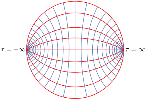
Figure 2: Curves of constant $\tau$ (in blue) and constant $\rho$ (in red) for AdS₂ stereographically projected to the unit disk (Poincaré disk). This shows how surfaces of constant $\tau$ converge to a boundary bound when $\tau\to-\infty$. The cartesian coordinates in the plane of the figure are given by $\vec{w}=\frac{(\cosh\rho\sinh\tau,\sinh\rho)}{1+\cosh\rho\cosh\tau}$ which puts the AdS₂ metric in the form $ds^{2}=\frac{4d\vec{w}^{2}}{1-\vec{w}^{2}}$.

The Hilbert space of the bulk theory can be decomposed in irreducible representations of the isometry group $SO(d+1,1)$. These are the highest weight representations of the conformal group, labelled by the scaling dimension and $SO(d)$ irrep of the the primary state. Therefore, the CFT conformal block decomposition of correlators follows from the partial wave decomposition in AdS, i.e. the decomposition in intermediate eigenstates of the Hamiltonian organized in irreps of the isometry group $SO(d+1,1)$. For example, the conformal block decomposition of the disconnected part of the four-point function,

$$\left\langle\mathcal{O}(P_{1})\dots\mathcal{O}(P_{4})\right\rangle=\frac{1}{\left(P_{12}P_{34}\right)^{\Delta}}+\frac{1}{\left(P_{13}P_{24}\right)^{\Delta}}+\frac{1}{\left(P_{14}P_{23}\right)^{\Delta}}\ ,$$ (89)

where $P_{ij}=-2P_{i}\cdot P_{j}$, is given by a sum of conformal blocks associated with the vacuum and two-particle intermediate states

$$\left\langle\mathcal{O}(P_{1})\dots\mathcal{O}(P_{4})\right\rangle=G_{0,0}(P_{1},\dots,P_{4})+\sum_{{l=0\atop even}}^{\infty}\sum_{n=0}^{\infty}c_{n,l}\,G_{2\Delta+2n+l,l}(P_{1},\dots,P_{4})\ .$$

Exercise 3.6

Check this statement in $d=2$ using the formula [28]

$$G_{E,l}(P_{1},P_{2},P_{3},P_{4})=\frac{k(E+l,z)k(E-l,\bar{z})+k(E-l,z)k(E+l,\bar{z})}{\left(-2P_{1}\cdot P_{2}\right)^{\Delta}\left(-2P_{3}\cdot P_{4}\right)^{\Delta}\left(1+\delta_{l,0}\right)}$$ (90)

where

$$k(2\beta,z)=(-z)^{\beta}\ _{2}F_{1}(\beta,\beta,2\beta,z)\ .$$ (91)

Determine the coefficients $c_{n,l}$ for $n\leq 1$ by matching the Taylor series expansion around $z=\bar{z}=0$. Extra: using a computer you can compute many coefficients and guess the general formula.

Generating function

There is an equivalent way of defining CFT correlation functions from QFT in AdS. We introduce the generating function

$$W\left[\phi_{b}\right]=\left\langle e^{\int_{\partial AdS}dP\phi_{b}(P)\mathcal{O}(P)}\right\rangle\ ,$$ (92)

where the integral over $\partial AdS$ denotes an integral over a chosen section of the null cone in $\mathbb{R}^{d+1,1}$ with its induced measure. We impose that the source obeys $\phi_{b}(\lambda P)=\lambda^{\Delta-d}\phi_{b}(P)$ so that the integral is invariant under a change of section, i.e. conformal invariant. For example, in the Poincaré section the integral reduces to $\int d^{d}x\phi_{b}(x)\mathcal{O}(x)$. Correlation functions are easily obtained with functional derivatives

$$\left\langle\mathcal{O}(P_{1})\dots\mathcal{O}(P_{n})\right\rangle=\left.\frac{\delta}{\delta\phi_{b}(P_{1})}\dots\frac{\delta}{\delta\phi_{b}(P_{n})}W\left[\phi_{b}\right]\right|_{\phi_{b}=0}\ .$$ (93)

If we set the generating function to be equal to the path integral over the field $\phi$ in AdS

$$W\left[\phi_{b}\right]=\frac{\int_{\phi\to\phi_{b}}\left[d\phi\right]e^{-S[\phi]}}{\int_{\phi\to 0}\left[d\phi\right]e^{-S[\phi]}}\ ,$$ (94)

with the boundary condition that it approaches the source $\phi_{b}$ at the boundary,

$$\lim_{\lambda\to\infty}\lambda^{d-\Delta}\phi(X=\lambda P+\dots)=\frac{1}{2\Delta-d}\frac{1}{\sqrt{C_{\Delta}}}\phi_{b}(P)\ ,$$ (95)

then we recover the correlation functions of $\mathcal{O}$ defined above as limits of the correlation functions of $\phi$.

For a quadratic bulk action, tha ratio of path intagrals in (94) is given $e^{-S}$ computed on the classical solution obeying the required boundary conditions. A natural guess for this solution is

$$\phi(X)=\sqrt{C_{\Delta}}\int_{\partial AdS}dP\frac{\phi_{b}(P)}{(-2P\cdot X)^{\Delta}}\ .$$ (96)

This automatically solves the AdS equation of motion $\nabla^{2}\phi=m^{2}\phi$, because it is an homogeneous function of weight $-\Delta$ and it obeys $\partial_{A}\partial^{A}\phi=0$ in the embedding space (see equations (61) and (63)). To see that it also obeys the boundary condition (95) it is convenient to use the Poincaré section.

Exercise 3.7

In the Poincaré section (29) and using Poincaré coordinates (48), formula (96) reads

$$\phi\left(z,x\right)=\sqrt{C_{\Delta}}\int d^{d}y\frac{z^{\Delta}\phi_{b}(y)}{\left(z^{2}+(x-y)^{2}\right)^{\Delta}}$$ (97)

and (95) reads

$$\lim_{z\to 0}z^{\Delta-d}\phi(z,x)=\frac{1}{2\Delta-d}\frac{1}{\sqrt{C_{\Delta}}}\phi_{b}(x)\ .$$ (98)

Show that (98) follows from (97). You can assume $2\Delta>d$.

The cubic term $\frac{1}{3!}g\phi^{3}$ in the action will lead to (calculable) corrections of order $g$ in the classical solution (96). To determine the generating function $W[\phi_{b}]$ in the classical limit we just have to compute the value of the bulk action (75) on the classical solution. However, before doing that, we have to address a small subtlety. We need to add a boundary term to the action (75) in order to have a well posed variational problem.

Exercise 3.8

The coefficient $\beta$ should be chosen such that the quadratic action

$$S_{2}=\int_{AdS}dw\sqrt{G}\left[\frac{1}{2}\left(\nabla\phi\right)^{2}+\frac{1}{2}m^{2}\phi^{2}\right]+\beta\int_{AdS}dw\sqrt{G}\,\nabla_{\alpha}\left(\phi\nabla^{\alpha}\phi\right)$$ (99)

is stationary around a classical solution obeying (98) for any variation $\delta\phi$ that preserves the boundary condition, i.e.

$$\delta\phi(z,x)=z^{\Delta}\left[f(x)+O(z)\right]\ .$$ (100)

Show that $\beta=\frac{\Delta-d}{d}$ and that the on-shell action is given by a boundary term

$$S_{2}=\frac{2\Delta-d}{2d}\int_{AdS}dw\sqrt{g}\,\nabla_{\alpha}\left(\phi\nabla^{\alpha}\phi\right)\ .$$ (101)

Finally, show that for the classical solution (97) this action is given by

$$S_{2}=-\frac{1}{2}\int d^{d}y_{1}d^{d}y_{2}\phi_{b}(y_{1})\phi_{b}(y_{2})K(y_{1},y_{2})\ ,$$ (102)

where

$$K(y_{1},y_{2}) =C_{\Delta}\frac{2\Delta-d}{d}\lim_{z\to 0}\int\frac{d^{d}x}{z^{d-1}}\frac{z^{\Delta}}{\left(z^{2}+(x-y_{1})^{2}\right)^{\Delta}}\partial_{z}\frac{z^{\Delta}}{\left(z^{2}+(x-y_{2})^{2}\right)^{\Delta}}$$

$$=\frac{1}{(y_{1}-y_{2})^{2\Delta}}$$ (103)

is the CFT two point function (77).

Exercise 3.9

Using $\phi=\phi_{0}+O(g)$ with $\phi_{0}$ given by (96), show that the complete on-shell action is given by

$$S=-\frac{1}{2}\int d^{d}y_{1}d^{d}y_{2}\phi_{b}(y_{1})\phi_{b}(y_{2})K(y_{1},y_{2})+\frac{1}{3!}g\int_{AdS}dX\left[\phi_{0}(X)\right]^{3}+O(g^{2})\ ,$$

and that this leads to the three-point function (78). Extra: Compute the terms of $O(g^{2})$ in the on-shell action.

We have seen that QFT on an AdS background naturally defines conformal correlation functions living on the boundary of AdS. Moreover, we saw that a weakly coupled theory in AdS gives rise to factorization of CFT correlators like in a large $N$ expansion. However, there is one missing ingredient to obtain a full-fledged CFT: a stress-energy tensor. In the next section, we will see that this requires dynamical gravity in AdS. The next exercise also shows that a free QFT in AdS_d+1 can not be dual to a local CFT_d.

Exercise 3.10

Compute the free-energy of a gas of free scalar particles in AdS. Since particles are free and bosonic one can create multi-particle states by populating each single particle state an arbitrary number of times. That means that the total partition function is a product over all single particle states and it is entirely determined by the single particle partition function. More precisely, show that

$$F=-T\log Z=-T\log\prod_{\psi_{sp}}\left(\sum_{k=0}^{\infty}q^{kE_{\psi_{sp}}}\right)=-T\sum_{n=1}^{\infty}\frac{1}{n}Z_{1}\left(q^{n}\right)\ ,$$ (104)

$$Z_{1}(q)=\sum_{\psi_{sp}}q^{E_{\psi_{sp}}}=\frac{q^{\Delta}}{(1-q)^{d}}\ ,$$ (105)

where $q=e^{-\frac{1}{RT}}$ and we have used the single-particle spectrum of the hamiltonian $D=-\frac{\partial}{\partial\tau}$ of AdS in global coordinates. Show that

$$F\approx-\zeta(d+1)R^{d}T^{d+1}$$ (106)

in the high temperature regime and compute the entropy using the thermodynamic relation $S=-\frac{\partial F}{\partial T}$. Compare this result with the expectation

$$S\sim(RT)^{d-1}\ ,$$ (107)

for the high temperature behaviour of the entropy of a CFT on a sphere $S^{d-1}$ of radius $R$. See section 4.3 of reference [29] for more details.

3 Gravity with AdS boundary conditions

Consider general relativity in the presence of a negative cosmological constant

$$I[G]=\frac{1}{\ell_{P}^{d-1}}\int d^{d+1}w\sqrt{G}\left[\mathcal{R}-2\Lambda\right]\ .$$ (108)

The AdS geometry

$$ds^{2}=R^{2}\frac{dz^{2}+dx_{\mu}dx^{\mu}}{z^{2}}\ ,$$ (109)

is a maximally symmetric classical solution with $\Lambda=-\frac{d(d-1)}{2R^{2}}$. When the AdS radius $R$ is much larger than the Planck length $\ell_{P}$ the metric fluctuations are weakly coupled and form an approximate Fock space of graviton states. One can compute the single graviton states and verify that they are in one-to-one correspondence with the CFT stress-tensor operator and its descendants (with AdS energies matching scaling dimensions). One can also obtain CFT correlation functions of the stress-energy tensor using Witten diagrams in AdS. The new ingredients are the bulk to boundary and bulk to bulk graviton propagators [30, 31, 32, 33, 34].

In the gravitational context, it is nicer to use the partition function formulation

$$Z[g_{\mu\nu},\phi_{b}]=\int_{{G\to g\atop\phi\to\phi_{b}}}\left[dG\right]\left[d\phi\right]e^{-I[G,\phi]}$$ (110)

where

$$I[G,\phi]=\frac{1}{\ell_{P}^{d-1}}\int d^{d+1}w\sqrt{G}\left[\mathcal{R}-2\Lambda+\frac{1}{2}\left(\nabla\phi\right)^{2}+\frac{1}{2}m^{2}\phi^{2}\right]$$ (111)

and the boundary condition are

$$ds^{2} = G_{\alpha\beta}dw^{\alpha}dw^{\beta}=R^{2}\frac{dz^{2}+dx^{\mu}dx^{\nu}\left[g_{\mu\nu}(x)+O(z)\right]}{z^{2}}\ ,$$ (112)

$$\phi = \frac{z^{d-\Delta}}{2\Delta-d}\left[\phi_{b}(x)+O(z)\right]\ .$$

By construction the partition function is invariant under diffeomorphisms of the boundary metric $g_{\mu\nu}$. Therefore, this definition implies the Ward identity (18). The generating function is also invariant under Weyl transformations

$$Z\left[\Omega^{2}g_{\mu\nu},\Omega^{\Delta-d}\phi_{b}\right]=Z\left[g_{\mu\nu},\phi_{b}\right]\qquad(naive)$$ (113)

This follows from the fact that the boundary condition

$$ds^{2} = R^{2}\frac{dz^{2}+dx^{\mu}dx^{\nu}\left[\Omega^{2}(x)g_{\mu\nu}(x)+O(z)\right]}{z^{2}}$$ (114)

$$\phi = \frac{z^{d-\Delta}}{2\Delta-d}\left[\Omega^{\Delta-d}(x)\phi_{b}(x)+O(z)\right]$$

can be mapped to (112) by the following coordinate transformation

$$z \to z\,\Omega-\frac{1}{4}z^{3}\Omega\left(\partial_{\mu}\log\Omega\right)^{2}+O(z^{5})$$ (115)

$$x^{\mu} \to x^{\mu}-\frac{1}{2}z^{2}\partial^{\mu}\log\Omega+O(z^{4})$$

where indices are raised and contracted using the metric $g_{\mu\nu}$ and its inverse. In other words, a bulk geometry that satisfies (112) also satisfies (114) with an appropriate choice of coordinates. If the partition function (110) was a finite quantity this would be the end of the story. However, even in the classical limit, where $Z\approx e^{-I}$, the partition function needs to be regulated. The divergences originate from the $z\to 0$ region and can be regulated by cutting off the bulk integrals at $z=\epsilon$ (as it happened for the scalar case discussed above). Since the coordinate transformation (115) does not preserve the cutoff, the regulated partition function is not obviously Weyl invariant. This has been studied in great detail in the context of holographic renormalization [35, 36]. In particular, it leads to the Weyl anomaly $g^{\mu\nu}T_{\mu\nu}\neq 0$ when $d$ is even. The crucial point is that this is a UV effect that does not affect the connected correlation functions of operators at separate points. In particular, the integrated form (LABEL:eq:WardIdentityFlux)=(22) of the conformal Ward identity is valid.

We do not now how to define the quantum gravity path integral in (110). The best we can do is a semiclassical expansion when $\ell_{P}\ll R$. This semiclassical expansion gives rise to connected correlators of the stress tensor $T_{\mu\nu}$ that scale as

$$\left\langle T_{\mu_{1}\nu_{1}}(x_{1})\dots T_{\mu_{n}\nu_{n}}(x_{n})\right\rangle_{c}\sim\left(\frac{R}{\ell_{P}}\right)^{d-1}\ .$$ (116)

This is exactly the scaling (45) we found from large $N$ factorization if we identify $N^{2}\sim\left(\frac{R}{\ell_{P}}\right)^{d-1}$. This suggests that CFTs related to semiclassical Einstein gravity in AdS, should have a large number of local degrees of freedom. This can be made more precise. The two-point function of the stress tensor in a CFT is given by

$$\left\langle T_{\mu\nu}(x)T_{\sigma\rho}(0)\right\rangle=\frac{C_{T}}{S_{d}^{2}}\frac{1}{x{}^{2d}}\left[\frac{1}{2}I_{\mu\sigma}I_{\nu\rho}+\frac{1}{2}I_{\mu\rho}I_{\nu\sigma}-\frac{1}{d}\delta_{\mu\nu}\delta_{\sigma\rho}\right]\ ,$$ (117)

where $S_{d}=\frac{2\pi^{d/2}}{\Gamma(d/2)}$ is the volume of a $(d-1)$-dimensional unit sphere and

$$I_{\mu\nu}=\delta_{\mu\nu}-2\frac{x_{\mu}x_{\nu}}{x^{2}}\ .$$ (118)

The constant $C_{T}$ provides an (approximate) measure of the number of degrees of freedom. For instance, for $n_{\varphi}$ free scalar fields and $n_{\psi}$ free Dirac fields we find [37]

$$C_{T}=n_{\varphi}\frac{d}{d-1}+n_{\psi}2^{\left[\frac{d}{2}\right]-1}d\ ,$$ (119)

where $\left[x\right]$ is the integer part of $x$. If the CFT is described by Einstein gravity in AdS, we find [30]

$$C_{T}=8\frac{d+1}{d-1}\frac{\pi^{\frac{d}{2}}\Gamma(d+1)}{\Gamma^{3}\left(\frac{d}{2}\right)}\frac{R^{d-1}}{\ell_{P}^{d-1}}\ ,$$ (120)

which shows that the CFT dual of a semiclassical gravitational theory with $R\gg\ell_{P}$, must have a very large number of degrees of freedom.

In summary, semiclassical gravity with AdS boundary conditions gives rise to a set of correlation functions that have all the properties (conformal invariance, Ward identities, large $N$ factorization) expected for the correlation functions of the stress tensor of a large $N$ CFT. Therefore, it is natural to ask if a CFT with finite $N$ is a quantum theory of gravity.

4 The AdS/CFT Correspondence

1 Quantum Gravity as CFT

What is quantum gravity? The most conservative answer is a standard quantum mechanical theory whose low energy dynamics around a weakly curved background is well described by general relativity (or some other theory with a dynamical metric). This viewpoint is particularly useful with asymptotically AdS boundary conditions. In this case, we can view the AdS geometry with a radius much larger than the Planck length as a background for excitations (gravitons) that are weakly coupled at low energies. Therefore, we just need to find a quantum system that reproduces the dynamics of low energy gravitons in a large AdS. In fact, we should be more precise about the word “reproduces”. We should define observables in quantum gravity that our quantum system must reproduce. This is not so easy because the spacetime geometry is dynamical and we can not define local operators. In fact, the only well defined observables are defined at the (conformal) boundary like the partition function (110) and the associated correlation functions obtained by taking functional derivatives. But in the previous section we saw that these observables have all the properties expected for the correlation functions of a large $N$ CFT. Thus, quantum gravity with AdS boundary conditions is equivalent to a CFT.

There are many CFTs and not all of them are useful theories of quantum gravity. Firstly, it is convenient to consider a family of CFTs labeled by $N$, so that we can match the bulk semiclassical expansion using $N^{2}\sim\left(\frac{R}{\ell_{P}}\right)^{d-1}$. In the large $N$ limit, every CFT single-trace primary operator of scaling dimension $\Delta$ gives rise to a weakly coupled field in AdS with mass $m\sim\Delta/R$. Therefore, if are looking for a UV completion of pure gravity in AdS without any other low energy fields, then we need to find a CFT where all single-trace operators have parametrically large dimension, except the stress tensor. This requires strong coupling and seems rather hard to achieve. Notice that a weakly coupled CFT with gauge group $SU(N)$ and fields in the adjoint representation has an infinite number of primary single-trace operators with order 1 scaling dimension. It is natural to conjecture that large $N$ factorization and correct spectrum of single-trace operators are sufficient conditions for a CFT to provide a UV completion of General Relativity (GR) [38]. However, this is not obvious because we still have to check if the CFT correlation functions of $T_{\mu\nu}$ match the prediction from GR in AdS. For example, the stress tensor three-point function is fixed by conformal symmetry to be a linear combination of 3 independent conformal invariant structures. On the other hand, the action (108) predicts a specific linear combination. It is not obvious that all large $N$ CFTs with the correct spectrum will automatically give rise to the same three-point function. There has been some recent progress in this respect. The authors of [39] used causality to show that this is the case. Unfortunately, their argument uses the bulk theory and can not be formulated entirely in CFT language. In any case, this is just the three-point fuction and GR predicts the leading large $N$ behaviour of all $n$-point functions. It is an important open problem to prove the following conjecture:

Any large N CFT where all single-trace operators, except the stress tensor, have parametrically large scaling dimensions, has the stress tensor correlation functions predicted by General Relativity in AdS.

Perhaps the most pressing question is if such CFTs exist at all. At the moment, we do not know the answer to this question but in the next section we will discuss closely related examples that are realized in the context of string theory.

If some CFTs are theories of quantum gravity, it is natural to ask if there are other CFT observables with a nice gravitational interpretation. One interesting example that will be extensively discussed in this school is the entanglement entropy of a subsystem. In section 3, we will discuss how CFT thermodynamics compares with black hole thermodynamics in AdS. In addition, in section 4 we will give several examples of QFT phenomena that have beautiful geometric meaning in the holographic dual.

2 String Theory

The logical flow presented above is very different from the historical route that led to the AdS/CFT correspondence. Moreover, from what we said so far AdS/CFT looks like a very abstract construction without any concrete examples of CFTs that have simple gravitational duals. If this was the full story probably I would not be writing these lecture notes. The problem is that we have stated properties that we want for our CFTs but we have said nothing about how to construct these CFTs besides the fact that they should be strongly coupled and obey large $N$ factorization. Remarkably, string theory provides a “method” to find explicit examples of CFTs and their dual gravitational theories.

The basic idea is to consider the low energy description of D-brane systems from the perspective of open and closed strings. Let us illustrate the argument by quickly summarizing the prototypical example of AdS/CFT [1]. Consider $N$ coincident D3-branes of type IIB string theory in 10 dimensional Minkowski spacetime. Closed strings propagating in 10 dimensions can interact with the D3-branes. This interaction can be described in two equivalent ways:

(a) D3-branes can be defined as a submanifold where open strings can end. This means that a closed string interacts with the D3-branes by breaking the string loop into an open string with endpoints attached to the D3-branes.

(b) D3-branes can be defined as solitons of closed string theory. In other words, they create a non-trivial curved background where closed strings propagate.

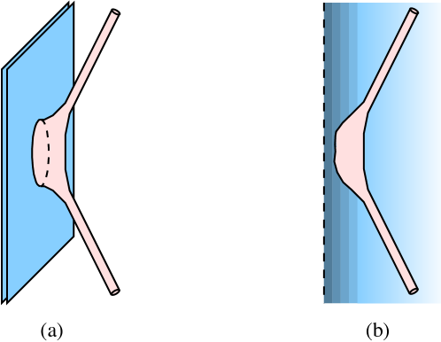
Figure 3: (a) Closed string scattering off branes in flat space. (b) Closed string propagating in a curved background.

These two alternatives are depicted in figure 3. Their equivalence is called open/closed duality. The AdS/CFT correspondence follows from the low-energy limit of open/closed duality. We implement this low-energy limit by taking the string length $\ell_{s}\to 0$, keeping the string coupling $g_{s}$, the number of branes $N$ and the energy fixed. In description (a), the low energy excitations of the system form two decoupled sectors: massless closed strings propagating in 10 dimensional Minkoski spacetime and massless open strings attached to the D3-branes, which at low energies are well described by $\mathcal{N}=4$ Supersymmetric Yang-Mills (SYM) with gauge group $SU(N)$. In description (b), the massless closed strings propagate in the following geometry

$$ds^{2}=\frac{1}{\sqrt{H(r)}}\eta_{\mu\nu}dx^{\mu}dx^{\nu}+\sqrt{H(r)}\left[dr^{2}+r^{2}d\Omega_{5}^{2}\right]\ ,$$ (121)

where $\eta_{\mu\nu}$ is the metric of the 4 dimensional Minkowski space along the branes and

$$H(r)=1+\frac{R^{4}}{r^{4}}\ ,\qquad R^{4}=4\pi g_{s}N\ell_{s}^{4}\ .$$ (122)

Naively, the limit $\ell_{s}\to 0$ just produces 10 dimensional Minkowski spacetime. However, one has to be careful with the region close to the branes at $r=0$. A local high energy excitation in this region will be very redshifted from the point of view of the observer at infinity. In order to determine the correct low-energy limit in the region around $r=0$ we introduce a new coordinate $z=R^{2}/r$, which we keep fixed as $\ell_{s}\to 0$. This leads to

$$ds^{2}=R^{2}\frac{dz^{2}+\eta_{\mu\nu}dx^{\mu}dx^{\nu}}{z^{2}}+R^{2}d\Omega_{5}^{2}\ ,$$ (123)

which is the metric of AdS${}_{5}\times S^{5}$ both with radius $R$. Therefore, description (b) also leads to 2 decoupled sectors of low energy excitations: massless closed strings in 10D and full type IIB string theory on AdS${}_{5}\times S^{5}$. This led Maldacena to conjecture that

$SU(N)$ SYM	$\Leftrightarrow$	IIB strings on AdS${}_{5}\times S^{5}$
$g_{YM}^{2}=4\pi g_{s}$		$\frac{R^{4}}{\ell_{s}^{4}}=g_{YM}^{2}N\equiv\lambda$

SYM is conformal for any value of $N$ and the coupling constant $g_{YM}^{2}$. The lagrangian of the theory involves the field strength

$$F_{\mu\nu}=\partial_{\mu}A_{\nu}-\partial_{\nu}A_{\mu}-i\left[A_{\mu},A_{\nu}\right]\ ,$$ (126)

6 scalars fields $\Phi^{m}$ and 4 Weyl fermions $\Psi^{a}$, which are all valued in the adjoint representation of $SU(N)$. The lagrangian is given by

$$\frac{1}{g_{YM}^{2}}{\rm Tr}\left[\frac{1}{4}F^{\mu\nu}F_{\mu\nu}+\frac{1}{2}\left(D^{\mu}\Phi^{m}\right)^{2}+\bar{\Psi}^{a}\sigma^{\mu}D_{\mu}\Psi_{a}\right.$$ (127)

$$\qquad\qquad\left.-\frac{1}{4}\left[\Phi^{m},\Phi^{n}\right]^{2}-C_{m}^{ab}\Psi_{a}\left[\Phi^{m},\Psi_{b}\right]-\bar{C}_{mab}\bar{\Psi}^{a}\left[\Phi^{m},\bar{\Psi}^{b}\right]\right]\ ,$$

where $D_{\mu}$ is the gauge covariant derivative and $C_{m}^{ab}$ and $\bar{C}_{mab}$ are constants fixed by the $SO(6)=SU(4)$ global symmetry of the theory. Notice that the isometry group of AdS${}_{5}\times S^{5}$ is $SO(5,1)\times SO(6)$, which matches precisely the bosonic symmetries of SYM: conformal group $\times$ global $SO(6)$. There are many interesting things to say about SYM. In some sense, SYM is the simplest interacting QFT in 4 dimensions [40]. However, this is not the focus of these lectures and we refer the reader to the numerous existing reviews about SYM [10, 41].

The remarkable conjecture of Maldacena has been extensively tested since it was first proposed in 1997 [1]. To test this conjecture one has to be able to compute the same observable on both sides of the duality. This is usually a very difficult task. On the SYM side, the regime accessible to perturbation theory is $g_{YM}^{2}N\ll 1$. This implies $g_{s}\ll 1$, which on the string theory side suppresses string loops. However, it also implies that the AdS radius of curvature $R$ is much smaller than the string length $\ell_{s}$. This means that the string worldsheet theory is very strongly coupled. In fact, the easy regime on the string theory side is $g_{s}\ll 1$ and $R\gg\ell_{s}$, so that (locally) strings propagate in an approximately flat space. Thus, directly testing the conjecture is a formidable task. There are three situations where a direct check can be made analitycally.

The first situation arises when some observable is independent of the coupling constant. In this case, one can compute it at weak coupling $\lambda\ll 1$ using the field theory description and at strong coupling $\lambda\gg 1$ using the string theory description. Usually this involves completely different techniques but in the end the results agree. Due to the large supersymmetry of SYM there are many observables that do not depend on the coupling constant. Notable examples include the scaling dimensions of half BPS single-trace operators and their three-point functions [42].

The second situation involves observables that depend on the coupling constant $\lambda$ but preserve enough supersymmetry that can be computed at any value of $\lambda$ using a technique called localization. Important examples of this type are the sphere partition function and the expectation value of circular Wilson loops [43, 44].

Finally, the third situation follows from the conjectured integrability of SYM in the planar limit. Assuming integrability one can compute the scaling dimension of non-protected single-trace operators at any value of $\lambda$ and match this result with SYM perturbative calculations for $\lambda\ll 1$ and with weakly coupled string theory for $\lambda\gg 1$ (see figure 1 from [45]). Planar scattering amplitudes an three-point functions of single-trace operators can also be computed using integrability [46, 47].

There are also numerical tests of the gauge/gravity duality. The most impressive study in this context, was the Monte-Carlo simulation of the BFSS matrix model [48] at finite temperature that reproduced the predictions from its dual black hole geometry [49, 50, 51, 52, 53, 54, 55].

How does the Maldacena conjecture fit into the general discussion of the previous sections? One important novelty is the presence of a large internal sphere on the gravitational side. We can perform a Kaluza-Klein reduction on $S^{5}$ and obtain an effective action for AdS₅

$$\frac{1}{(2\pi)^{7}\ell_{s}^{8}}\int d^{10}x\sqrt{g_{10}}e^{-2\Phi}\left[\mathcal{R}_{10}+\dots\right]\to\frac{R^{5}}{8(2\pi)^{4}g_{s}^{2}\ell_{s}^{8}}\int d^{5}x\sqrt{g_{5}}\left[\mathcal{R}_{5}+\dots\right]\ .$$

This allows us to identify the 5 dimensional Planck length

$$\ell_{P}^{3}=\frac{8(2\pi)^{4}g_{s}^{2}\ell_{s}^{8}}{R^{5}}$$ (128)

and verify the general prediction $N^{2}\sim R^{3}/\ell_{P}^{3}$ . Remarkably, at strong coupling $\lambda\gg 1$ all single-trace non-protected operators of SYM have parametrically large scaling dimensions. This is simple to understand from the string point of view. Massive string states have masses $m\sim 1/\ell_{s}$. But we saw in the previous sections that the dual operator to an AdS field of mass $m$ has a scaling dimension $\Delta\sim mR\sim R/\ell_{s}\sim\lambda^{\frac{1}{4}}$. The only CFT operators that have small scaling dimension for $\lambda\gg 1$ are dual to massless string states that constitute the fields of type IIB supergravity (SUGRA). Therefore, one can say that SYM (with $N\gg\lambda\gg 1$) provides a UV completion of IIB SUGRA with AdS${}_{5}\times S^{5}$ boundary conditions.

String theory provides more concrete examples of AdS/CFT dual pairs. These examples usually involve SCFTs (or closely related non-supersymmetry theories). This is surprising because SUSY played no role in our general discussion. At the moment, it is not known if SUSY is an essential ingredient of AdS/CFT or if it is only a useful property that simplifies the calculations. The latter seems more likely but notice that SUSY might be essential to stabilize very strong coupling and allow the phenomena of large scaling dimensions for almost all single-trace operators. Another observation is that it turns out to be very difficult to construct AdS duals with small internal spaces (for SYM we got a 5-sphere with the same radius of AdS₅). It is an open problem to find CFTs with gravity duals in less than 10 dimensions (see [56, 57] for attempts in this direction).

Another interesting class of examples are the dualities between vector models and Higher Spin Theories (HST) [58, 59]. Consider for simplicity the free $O(n)$ model in 3 dimensions

$$S=\int d^{3}x\sum_{i=1}^{n}\frac{1}{2}\partial_{\mu}\varphi^{i}\partial^{\mu}\varphi^{i}\ .$$ (129)

In this case, the analogue of single-trace operators are the $O(n)$ singlets $\mathcal{O}_{l}=\sum_{i}\varphi^{i}\partial_{\mu_{1}}\dots\partial_{\mu_{l}}\varphi^{i}$ with even spin $l$ and dimension $\Delta=1+l$. At large $n$, the correlation functions of these operators factorize with $n$ playing the role of $N^{2}$ in a $SU(N)$ gauge theory with adjoint fields. The AdS dual of this CFT is a theory with one massless field for each even spin. These theories are rather non-local and they can not be defined in flat spacetime. Even if we introduce the relevant interaction $\left(\varphi^{i}\varphi^{i}\right)^{2}$ and flow to the IR fixed point (Wilson-Fisher fixed point), the operators $\mathcal{O}_{l}$ with $l>2$ get anomalous dimensions of order $\frac{1}{n}$ and therefore the classical AdS theory still contains the same number of massless higher spin fields. This duality has been extended to theories with fermions and to theories where the global $O(n)$ symmetry is gauged using Chern-Simons gauge fields. It is remarkable that HST in AdS seems to have the correct structure to reproduce the CFT observables that have been computed so far. Notice that in these examples of AdS/CFT supersymmetry plays no role. However, it is unclear if the AdS description is really useful in this case. In practice, the large $n$ limit of these vector models is solvable and the dual HST in AdS is rather complicated to work with even at the classical level. There are also analogous models in AdS₃/CFT₂ duality [62].

3 Finite Temperature

In section 3, we argued that holographic CFTs must have a large number of local degrees of freedom, using the two-point function of the stress tensor. Another way of counting degrees of freedom is to look at the entropy density when the system is put at finite temperature. For a CFT in flat space and infinite volume, the temperature dependence of the entropy density is fixed by dimensional analysis because there is no other scale available,

$$s=c_{s}T^{d-1}\ .$$ (130)

The constant $c_{s}$ is a physical measure of the number of degrees of freedom.

The gravitational dual of the system at finite temperature is a black brane in asymptotically AdS space. The Euclidean metric is given by

$$ds^{2}=\frac{R^{2}}{z^{2}}\left[\frac{dz^{2}}{1-(z/z_{H})^{d}}+\left(1-\frac{z^{d}}{z_{H}^{d}}\right)d\tau^{2}+\delta_{ij}dx^{i}dx^{j}\right]\ .$$ (131)

Exercise 4.1

Show that in order to avoid a conical defect at the horizon $z=z_{H}$, we need to identify Euclidean time $\tau$ with period $\frac{4\pi z_{H}}{d}$. This fixes the Hawking temperature $T=\frac{d}{4\pi z_{H}}$.

The formula $T=\frac{d}{4\pi z_{H}}$ illustrates a general phenomena in holography: high energy corresponds to the region close to the boundary and low energy corresponds to the deep interior of the dual geometry.

The entropy of the system is given by the Bekenstein-Hawking formula

$$S=\frac{A_{H}}{4G_{N}}=\frac{4\pi}{\ell_{P}^{d-1}}\frac{R^{d-1}}{z_{H}^{d-1}}\int d^{d-1}x\qquad\Rightarrow\qquad c_{s}=\frac{(4\pi)^{d}}{d^{d-1}}\frac{R^{d-1}}{\ell_{P}^{d-1}}\ .$$ (132)

As expected $c_{s}$ is very large in the bulk classical limit $R\gg\ell_{P}$. Interestingly, the ratio

$$\frac{c_{s}}{C_{T}}=\frac{\pi^{\frac{d}{2}}}{8}\left(\frac{4}{d}\right)^{d}\frac{d-1}{d+1}\frac{\Gamma^{3}\left(\frac{d}{2}\right)}{\Gamma(d)}$$ (133)

only depends on the spacetime dimension $d$ if the CFT has a classical bulk dual [63]. It would be very nice to prove that all large $N$ CFTs where all single-trace operators, except the stress tensor, have parametrically large scaling dimensions, satisfy (133). Notice that (133) is automatic in $d=2$ because $C_{T}=2c$ and $c_{s}=\frac{\pi}{3}c$ are uniquely fixed in terms of the central charge $c$. In planar SYM, $C_{T}=40N^{2}$ is independent of the ’t Hooft coupling but $c_{s}$ varies with $\lambda$ (although not much, $c_{s}(\lambda=\infty)=\frac{3}{4}c_{s}(\lambda=0)$). In this case, (133) is only satisfied at strong coupling, when all primary operators with spin greater than 2 have parametrically large scaling dimensions.

Exercise 4.2

Consider a CFT on a sphere of radius $L$ and at temperature $T$. In this case, the entropy is a non-trivial function of the dimensioless combination $LT$. Let us compute this function assuming the CFT is well described by Einstein gravity with asymptotically AdS boundary conditions. There are two possible bulk geometries that asymptote to the Euclidean boundary $S^{1}\times S^{d-1}$. The first is pure AdS

$$ds^{2}=R^{2}\left[\frac{dr^{2}}{1+r^{2}}+\left(1+r^{2}\right)d\tau^{2}+r^{2}d\Omega_{d-1}^{2}\right]$$ (134)

with Euclidean time periodically identified and the second is Schwarzschild-AdS

$$ds^{2}=R^{2}\left[\frac{dr^{2}}{f(r)}+f(r)d\tilde{\tau}^{2}+r^{2}d\Omega_{d-1}^{2}\right]\ ,$$ (135)

where $f(r)=1+r^{2}-\frac{m}{r^{d-2}}$. At the boundary $r=r_{max}\gg 1$, both solutions should be conformal to $S^{1}\times S^{d-1}$ with the correct radii. Show that this fixes the periodicities

$$\Delta\tau=\frac{1}{TL}\frac{r_{max}}{\sqrt{1+r_{max}^{2}}}\ ,\qquad\Delta\tilde{\tau}=\frac{1}{TL}\frac{r_{max}}{\sqrt{f(r_{max})}}\ .$$ (136)

Show also that regularity of the metric (135) implies the periodicity

$$\Delta\tilde{\tau}=\frac{4\pi}{f^{\prime}(r_{H})}=\frac{4\pi}{r_{H}d+\frac{d-2}{r_{H}}}\ ,$$ (137)

where $r=r_{H}$ is the largest zero of $f(r)$. Notice that this implies a minimal temperature for Schwarzschild black holes in AdS, $T>\frac{\sqrt{d(d-2)}}{2\pi L}$.

Both (134) and (135) are stationary points of the Euclidean action (108). Therefore, we must compute the value of the on-shell action in order to decide which one dominates the path integral. Show that the difference of the on-shell actions is given by

$$I_{BH}-I_{AdS} =-2S_{d}\frac{R^{d-1}}{\ell_{P}^{d-1}}\left[r_{max}^{d}\Delta\tau-\left(r_{max}^{d}-r_{H}^{d}\right)\Delta\tilde{\tau}\right]$$ (138)

$$\longrightarrow S_{d}\frac{R^{d-1}}{\ell_{P}^{d-1}}\frac{1}{TL}r_{H}^{d-2}(1-r_{H}^{2})$$ (139)

where $S_{d}$ is the area of a unit $(d-1)$-dimensional sphere and in the last step we took the limit $r_{max}\to\infty$. Conclude that the black hole only dominates the bulk path integral when $r_{H}>1$, which corresponds to $T>\frac{d-1}{2\pi L}$. This is the Hawking-Page phase transition [64]. It is natural to set the free-energy of the AdS phase to zero because this phase corresponds to a gas of gravitons around the AdS background whose free energy does not scale with the large parameter $(R/\ell_{P})^{d-1}$. Therefore, the free energy of the black hole phase is given by

$$F_{BH}=\frac{1}{L}S_{d}\frac{R^{d-1}}{\ell_{P}^{d-1}}r_{H}^{d-2}(1-r_{H}^{2})\ .$$ (140)

Verify that the thermodynamic relation $\frac{\partial F}{\partial T}=-S$ agrees with the Bekenstein-Hawking formula for the black hole entropy. Since this a first order phase transition you can also compute its latent heat.

In the last exercise, we saw that for a holographic CFT on a sphere of radius $L$, the entropy is a discontinuous function of the temperature. In fact, we found that for sufficiently high temperatures $T>\frac{d-1}{2\pi L}$, the entropy was very large $S\sim C_{T}$, while for lower temperatures the entropy was small because it did not scale with $C_{T}$. This can be interpreted as deconfinement of the numerous degrees of freedom measured by $C_{T}\gg 1$ which do not contribute to the entropy below the transition temperature $T_{c}=\frac{d-1}{2\pi L}$. How can this bevavior be understood from the point of view of a large $N$ gauge CFT?

4 Applications

The AdS/CFT correspondence (or the gauge/gravity duality more generally) is a useful framework for thinking about strong coupling phenomena in QFT. Besides the specific examples of strongly coupled CFTs that can be studied in great detail using the gravitational dual description, AdS/CFT provides a geometric reformulation of many effects in QFT. Usually, we do not know the precise gravitational dual of a given QFT of interest (like QCD) but it is still very useful to study gravitational toy models that preserve the main features we are interested in. These models enlarge our intuition because they are very different from QFT models based on weakly interacting quasi-particles. There are many examples of QFT observables that have a nice geometric interpretation in the dual gravitational description. Perhaps the most striking one is the computation of entanglement entropy as the area of a minimal surface in the dual geometry [65]. Let us illustrate this approach in the context of confinig gauge theories like pure Yang-Mills theory.

Confinement means that the quark anti-quark potential between static quarks grows linearly with the distance $L$ at large distances

$$V(L)\approx\sigma L\ ,\qquad L\to\infty\ ,$$ (141)

where $\sigma$ is the tension of the flux tube or effective string. This potential can be defined through the expectation value of a Wilson loop (in the fundamental representation)

$$W[C]={\rm Tr\ P}\exp\oint_{C}A_{\mu}dx^{\mu}\ ,$$ (142)

for a rectangular contour $C$ with sides $T\times L$,

$$\left\langle W[C]\right\rangle\sim e^{-TV(L)}\ ,\qquad T\to\infty\>.$$ (143)

This is equivalent to the area law $\left\langle W[C]\right\rangle\sim e^{-\sigma Area[C]}$ for large contours. In the gauge/string duality there is a simple geometric rule to compute expectation values of Wilson loops [66]. One should evaluate the path integral

$$\left\langle W[C]\right\rangle=\int_{\partial\Sigma=C}[d\Sigma]e^{-S_{s}[\Sigma]}$$ (144)

summing over all surfaces $\Sigma$ in the dual geometry that end at the contour $C$ at the boundary. The path integral is weighted using the dual string world-sheet action. At large $N$, we expect that the dominant contribution comes from surfaces $\Sigma$ with disk topology. In specific examples, like SYM, this can be made very precise. For example, at large ’t Hooft coupling the world-sheet action reduces to

$$S_{s}[\Sigma]=\frac{1}{4\pi\ell_{s}^{2}}Area[\Sigma]\ .$$ (145)

In this case, since the theory is conformal, there is no confinement and the quark anti-quark potential is Coulomb like,

$$V(L)=\frac{a(N,\lambda)}{L}\ .$$ (146)

For most confining gauge theories (e.g. pure Yang-Mills theory) we do not know neither the dual geometry nor the dual string world-sheet action. However, we can get a nice qualitative picture if we assume (145) and only change the background geometry. The most general $(d+1)$-dimensional geometry that preserves $d$-dimensional Poincaré invariance can be written as

$$ds^{2}=R^{2}\left[\frac{dz^{2}}{z^{2}}+A^{2}(z)dx^{\mu}dx_{\mu}\right]\ .$$ (147)

The profile of the function $A^{2}(z)$ encodes many properties of the dual QFT. For a CFT, scale invariance fixes $A(z)\propto z^{-1}$. For asymptotically free gauge theories, we still expect that $A(z)$ diverges for $z\to 0$ however the function should be very different for larger values of $z$. In particular, it should have a minimum for some value $z=z_{\star}>0$. Let us see what this implies for the expectation value of a large Wilson loop. The string path integral (144) will be dominated by the surface $\Sigma$ with minimal area. For large contours $C$, this surface will sink inside AdS until the value $z=z_{\star}$ that minimizes $A^{2}(z)$ and the worldsheet area will be given by

$$R^{2}A^{2}(z_{\star})Area[C]+O(Length[C])\ .$$ (148)

Therefore, we find a confining potential with flux tube tension

$$\sigma=\frac{A^{2}(z_{\star})}{4\pi}\frac{R^{2}}{\ell_{s}^{2}}\ .$$ (149)

What happens if we put the QFT at finite temperature? In this case, we can probe confinement by computing

$$\left\langle W(C_{x})\bar{W}(C_{x+L})\right\rangle_{\beta}=e^{-\beta F_{q\bar{q}}(\beta,L)}$$ (150)

where $C_{x}$ is the contour around the Euclidean time circle at the spatial position $x$ (Polyakov loop). $F_{q\bar{q}}(\beta,L)$ denotes the free energy of a static quark anti-quark pair at distance $L$ and temperature $1/\beta$. If $F_{q\bar{q}}(\beta,L)\to\infty$ as we separate the pair, then we are in the confined phase. On the other hand, if $F_{q\bar{q}}(\beta,L)$ remains finite when $L\to\infty$, we are in the deconfined phase. Let us see how this works in the holographic dual. For low temperatures, the dual geometry is simply given by (147) with Euclidean time identified with period $\beta.$ Therefore, the bulk minimal surface that ends on $C_{x}$ and $C_{x+L}$ will have a cylindrical topology and its area will scale linearly with $L$ at large $L$. In fact, we find $F_{q\bar{q}}(\beta,L)\approx\sigma L$ like in the vacuum. On the other hand, for high enough temperature we expect the bulk path integral to be dominated by a black hole geometry (see exercise 4.2 about Hawking-Page phase transition). The metric can then be written as

$$ds^{2}=R^{2}\left[\frac{dz^{2}}{z^{2}f(z)}+f(z)d\tau^{2}+g(z)dx^{i}dx_{i}\right]\ ,$$ (151)

where $f(z)$ vanishes for some value $z=z_{H}$. This means that the Euclidean time circle is contractible in the bulk. Therefore, for large $L$, the minimal surface has two disconnected pieces with disk topology ending on $C_{x}$ and $C_{x+L}$ whose area remains finite when $L\to\infty$. This means deconfinement

$$\lim_{L\to\infty}\left\langle W(C_{x})\bar{W}(C_{x+L})\right\rangle_{\beta}=\left\langle W(C_{x})\right\rangle_{\beta}^{2}=e^{-2\beta F_{q}(\beta)}>0\ .$$ (152)

Another feature of a confining gauge theory is a mass gap and a discrete spectrum of mesons and glueballs. To compute this spectrum using the bulk dual one should study fluctuations around the vacuum geometry (147). Consider for simplicity, a scalar field obeying $\nabla^{2}\phi=m^{2}\phi$. Since we are interested in finding the spectrum of the operator $P_{\mu}P^{\mu}$ we look for solutions of the form $\phi=e^{ik\cdot x}\psi(z)$, which leads to

$$\frac{z}{A^{d}(z)}\partial_{z}\left(zA^{d}(z)\partial_{z}\psi\right)-\frac{k^{2}}{A^{2}(z)}\psi=m^{2}R^{2}\psi\ .$$ (153)

The main idea is that this equation will only have solutions that obey the boundary conditions $\psi(0)=\psi(\infty)=0$ for special discrete values of $k^{2}$. In other words, we obtain a discrete mass spectrum as expected for a confining gauge theory.

Exercise 4.3

Consider the simplest holographic model of a confining gauge theory: the hard wall model. This is just a slice of AdS, i.e. we take $A(z)=1/z$ and cutoff space at $z=z_{\star}$. Show that (153) reduces to the Bessel equation

$$\left[z^{2}\partial_{z}^{2}+z\partial_{z}-\alpha^{2}-k^{2}z^{2}\right]h(z)=0\ ,$$ (154)

where $\alpha^{2}=m^{2}R^{2}+d^{2}/4$ and $h(z)=z^{-\frac{d}{2}}\psi(z)$. Finally, show that the boundary conditions $h(0)=h(z_{\star})=0$, lead to the quantization

$$h_{n}(z)=J_{\alpha}\left(\frac{z}{z_{\star}}u_{\alpha,n}\right)\ ,\qquad m_{n}^{2}=-k^{2}=\frac{u_{\alpha,n}^{2}}{z_{\star}^{2}}\ ,\qquad n=1,2,\dots$$ (155)

where $u_{\alpha,n}$ is the $n$th zero of the Bessel function $J_{\alpha}$.

It is instructive to compare the lightest glueball mass $m_{1}$ with the flux tube tension $\sigma=\frac{1}{4\pi z_{\star}^{2}}\frac{R^{2}}{\ell_{s}^{2}}$ in the hard wall model. We find that $\frac{\sigma}{m_{1}^{2}}\sim\frac{R^{2}}{\ell_{s}^{2}}$. The fact that this ratio is of order 1 in pure Yang-Mills theory is another indication that its holographic dual must be very stringy (curvature radius of the same order of the string length).

Above the deconfinement temperature, the system is described by a plasma of deconfined partons (quarks and gluons in QCD). The gauge/gravity duality is also very useful to describe this strongly coupled plasma. The idea is that the hydrodynamic behavior of the plasma is dual to the long wavelength fluctuations of the black hole horizon. This map can be made very precise and has led to significant developments in the theory of relativistic hydrodynamics. One important feature of the gravitational description is that dissipation is built in because black hole horizons naturally relax to equilibrium. A famous result from this line of work was the discovery of a universal ratio of shear viscosity $\eta$ to entropy density $s$. Any CFT dual to Einstein gravity in AdS has $\frac{\eta}{s}=\frac{1}{4\pi}$. This is a rather small number (water at room temperature has $\frac{\eta}{s}\sim 30$) but remarkably it is of the same order of magnitude of that observed in the quark-gluon plasma produced in heavy ion collisions [67].

There are also many interesting applications of the gauge/gravity duality to Condensed Matter physics [14, 9]. There are many materials that are not well described by weakly coupled quasi-particles. In this case, it is useful to have alternative models based on gravitational theories in AdS that share the same qualitative features. This can give geometric intuition about the system in question.

The study of holographic models is also very useful for the discovery of general properties of CFT (and QFT more generally). If one observes that a given property holds both in weakly coupled and in holographic CFTs, it is natural to conjecture that such property holds in all CFTs. This reasoning has led to the discovery (and sometimes proof) of several important facts about CFTs, like the generalization of Zamolodchikov’s c-theorem to $d>2$ (known as F-theorem in $d=3$ and a-theorem in $d=4$) [68, 69, 70, 71] or the existence of universal bounds on the three-point function of the stress tensor and its relation to the idea of energy correlators [72, 73, 74].

Onother example along this line is the existence of “double-trace” operators with large spin in any CFT. The precise statement is that in the OPE of two operators $\mathcal{O}_{1}$ and $\mathcal{O}_{2}$ there is an infinite number of operators $\mathcal{O}_{n,l}$ of spin $l\gg 1$ and scaling dimension

$$\Delta_{n,l}\approx\Delta_{1}+\Delta_{2}+2n+l+\frac{\gamma_{n}}{l^{\tau_{min}}}$$ (156)

where $\tau_{min}$ is the minimal twist (dimension minus spin) of all the operators that appear in both OPEs $\mathcal{O}_{1}\times\mathcal{O}_{1}$ and $\mathcal{O}_{2}\times\mathcal{O}_{2}$. In a generic CFT, this will be the stress tensor with $\tau_{min}=d-2$ and one can derive explicit formulas for $\gamma_{n}$ [75, 76, 77, 78]. This statement has been proven using the conformal bootstrap equations but its physical meaning is more intuitive in the dual AdS language. Consider two particle primary states in AdS. Without interactions the energy of such states is given by $\Delta_{1}+\Delta_{2}+2n+l$ where $n=0,1,2,\dots$ is a radial quantum number and $l$ is the spin. Turning on interactions will change the energies of these two-particle states. However, the states with large spin and fixed $n$ correspond to two particles orbitating each other at large distances and therefore they will suffer a small energy shift due to the gravitational long range force. At large spin, all other interactions (corresponding to operators with higher twist) give subdominant contributions to this energy shift. In other words, the general result (156) is the CFT reflection of the simple fact that interactions decay with distance in the dual AdS picture.

5 Mellin amplitudes

Correlation functions of local operators in CFT are rather complicated functions of the cross-ratios. Since these are crucial observables in AdS/CFT it is useful to find simpler representations. This is the motivation to study Mellin amplitudes. They were introduced by G. Mack in 2009 [79, 80] following earlier work [81, 82]. Mellin amplitudes share many of the properties of scattering amplitudes of dual resonance models. In particular, they are crossing symmetric and have a simple analytic structure (related to the OPE). As we shall see, in the case of holographic CFTs, we can take this analogy further and obtain bulk flat space scattering amplitudes as a limit of the dual CFT Mellin amplitudes. Independently of AdS/CFT applications, Mellin amplitudes can be useful to describe CFTs in general.

1 Definition

Consider the $n$-point function of scalar primary operators

$$\left\langle\mathcal{O}_{1}(P_{1})\dots\mathcal{O}_{n}(P_{n})\right\rangle=\int[d\gamma]M(\gamma_{ij})\prod_{1\leq i<j\leq n}\frac{\Gamma(\gamma_{ij})}{(-2P_{i}\cdot P_{j})^{\gamma_{ij}}}$$ (157)

Conformal invariance requires weight $-\Delta_{i}$ in each $P_{i}$. This leads to constraints in the Mellin variables which can be conveniently written as

$$\sum_{j=1}^{n}\gamma_{ij}=0\ ,\qquad\gamma_{ij}=\gamma_{ji}\ ,\qquad\gamma_{ii}=-\Delta_{i}\ .$$ (158)

Notice that for $n=2$ and $n=3$ the Mellin variables are entirely fixed by these constraints. In these cases, there is no integral to do and the Mellin representation just gives the known form of the conformal two and three point function. The integration measure $[d\gamma]$ is over the $n(n-3)/2$ independent Mellin variables (including a factor of $\frac{1}{2\pi i}$ for each variable) and the integration contours run parallel to the imaginary axis. The precise contour in the complex plane is dictated by the requirement that it should pass to the right/left of the semi-infinite sequences of poles of the integrand that run to the left/right. This will become clear in the following example.

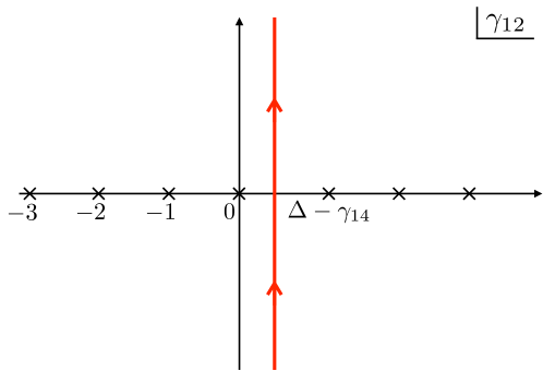
Figure 4: Integration contour for the Mellin variable $\gamma_{12}$. The crosses represent (double) poles of the $\Gamma$-functions given by (161) and (162). In general, the Mellin amplitude has several semi-infinite sequence of poles. Each sequence should stay entirely on one side of the contour.

Consider the case of a four-point function of a scalar operator of dimension $\Delta$. In this case, there are two independent Mellin variables which we can choose to be $\gamma_{12}$ and $\gamma_{14}$. This leads to

$$\left\langle\mathcal{O}(P_{1})\dots\mathcal{O}(P_{4})\right\rangle=\frac{1}{(P_{13}P_{24})^{\Delta}}\int_{-i\infty}^{i\infty}\frac{d\gamma_{12}\gamma_{14}}{(2\pi i)^{2}}\hat{M}(\gamma_{12},\gamma_{14})u^{-\gamma_{12}}v^{-\gamma_{14}}\,,$$ (159)

where $u$ and $v$ are the cross ratios (11) and

$$\hat{M}(\gamma_{12},\gamma_{14})=M(\gamma_{12},\gamma_{14})\Gamma^{2}(\gamma_{12})\Gamma^{2}(\gamma_{14})\Gamma^{2}(\Delta-\gamma_{12}-\gamma_{14})\,.$$ (160)

Consider the first the complex plane of $\gamma_{12}$ depicted in figure 4. The $\Gamma$-functions give rise to semi-infinite sequences of (double) poles at

$$\gamma_{12} =0,-1,-2,\dots$$ (161)

$$\gamma_{12} =\Delta-\gamma_{14},\Delta-\gamma_{14}+1,\Delta-\gamma_{14}+2,\dots$$ (162)

As we shall see in the next section, the Mellin amplitude $M(\gamma_{ij})$ also has the same type of semi-infinite sequences of poles. The integration contour should pass in the middle of these sequences of poles as shown in figure 4. Invariance of the four-point function under permutation of the insertion points $P_{i}$, leads to crossing symmetry of the Mellin amplitude

$$M(\gamma_{12},\gamma_{13},\gamma_{14})=M(\gamma_{13},\gamma_{12},\gamma_{14})=M(\gamma_{14},\gamma_{13},\gamma_{12})\ ,$$ (163)

where we used 3 variables obeying a single constraint $\gamma_{12}+\gamma_{13}+\gamma_{14}=\Delta$. This is reminiscent of crossing symmetry of scattering amplitudes written in terms of Mandelstam invariants.

It is convenient to introduce fictitious momenta $p_{i}$ such that $\gamma_{ij}=p_{i}\cdot p_{j}$. Imposing momentum conservation $\sum_{i=1}^{n}p_{i}=0$ and the on-shell condition $p_{i}^{2}=-\Delta_{i}$ automatically leads to the constraints (158). These fictitious momenta are a convenient trick but we do not know how to define them directly. In all formulas, we will only use their inner products $\gamma_{ij}=p_{i}\cdot p_{j}$. In particular, it is not clear in what vector space do the momenta $p_{i}$ live.

Let us be more precise about the number of independent cross ratios. The correct formula is

$$\frac{n(n-3)}{2}\ ,\qquad n\leq d+2$$ (164)

$$nd-\frac{(d+1)(d+2)}{2}\ ,\qquad n\geq d+2$$ (165)

In fact, for $n>d+2$ one can write identities like

$$\det_{i,j}P_{i}\cdot P_{j}=0$$ (166)

using $d+3$ embedding space vectors. Notice that this makes the Mellin representation non-unique. We can shift the Mellin amplitude by the Mellin transform of

$$F(P_{1},\dots,P_{n})\det_{i,j}P_{i}\cdot P_{j}=0$$ (167)

where $F$ is any scalar function with the appropriate homogeneity properties. This non-uniqueness of the Mellin amplitude is analogous to the non-uniqueness of the $n$-particle scattering amplitudes (as functions of the invariants $k_{i}\cdot k_{j}$) in $(d+1)$-dimensional spacetime if $n>d+2$.

2 OPE $\Rightarrow$ Factorization

Consider the OPE

$$\mathcal{O}_{1}(x_{1})\mathcal{O}_{1}(x_{2})=\sum_{k}C_{12k}\left(x_{12}^{2}\right)^{\frac{\Delta_{k}-\Delta_{1}-\Delta_{2}}{2}}\left[\mathcal{O}_{k}(x_{2})+c\,x_{12}^{2}\partial^{2}\mathcal{O}_{k}(x_{2})+\dots\right]$$ (168)

where the sum is over primary operators $\mathcal{O}_{k}$ and, for simplicity, we wrote the contribution of a scalar operator. The term proportional to the constant $c$ is a descendant and is fixed by conformal symmetry like all the other terms represented by $\dots$. Let us compare this with the Mellin representation. When $x_{12}^{2}\to 0$, it is convenient to integrate over $\gamma_{12}$ closing the contour to the left in the $\gamma_{12}$-complex plane. This gives

$$\langle\mathcal{O}_{1}(x_{1})\mathcal{O}_{1}(x_{2})\dots\rangle=\sum_{\bar{\gamma}_{12}}\left(x_{12}^{2}\right)^{-\bar{\gamma}_{12}}\int[d\gamma]^{\prime}{\rm Res}_{\bar{\gamma}_{12}}\hat{M}(\gamma_{ij})\prod^{\prime}\left(x_{ij}^{2}\right)^{-\gamma_{ij}}$$ (169)

where $[d\gamma]^{\prime}$ and $\prod^{\prime}$ stand for the integration measure and product excluding $ij=12$. Comparing the two expressions we conclude that $\hat{M}$ must have poles at

$$\gamma_{12}=\frac{\Delta_{1}+\Delta_{2}-\Delta_{k}-2m}{2}\ ,\qquad\qquad m=0,1,2,\dots$$ (170)

where the poles with $m>0$ correspond to descendant contributions. If the CFT has a discrete spectrum of scaling dimensions then its Mellin amplitudes are analytic functions with single poles as its only singularities (meromorphic functions). It is also clear that the residues of these poles will be proportional to the product of the OPE coefficient $C_{12k}$ and the Mellin amplitude of the lower point correlator $\langle\mathcal{O}_{k}\dots\rangle$. The precise formulas are derived in [79, 83]. Here we shall just list the main results without derivation.

Four-point function

In the case of the four-point function it is convenient to write the Mellin amplitude in terms of ‘Mandelstam invariants’

$$s =-(p_{1}+p_{2})^{2}=\Delta_{1}+\Delta_{2}-2\gamma_{12}$$ (171)

$$t =-(p_{1}+p_{3})^{2}=\Delta_{1}+\Delta_{3}-2\gamma_{13}$$ (172)

Then, the poles and residues of the Mellin amplitude take the following form [79]

$$M(s,t)\approx C_{12k}C_{34k}\frac{Q_{l_{k},m}(t)}{s-\Delta_{k}+l_{k}-2m}\ ,\qquad m=0,1,2,\dots$$ (173)

where $Q_{l,m}(t)$ is a kinematical polynomial of degree $l$ in the variable $t$.

This strengthens the analogy with scattering amplitudes. Each operator of spin $l$ in the OPE $\mathcal{O}_{1}\times\mathcal{O}_{2}$ gives rise to poles in the Mellin amplitude very similar to the poles in the scattering amplitude associated to the exchange of a particle of the same spin.

Planar correlators

Notice that the polynomial behaviour of the residues requires the inclusion of the $\Gamma$-functions in the definition (157) of Mellin amplitudes. On the other hand, the $\Gamma$-functions themselves have poles at fixed positions. For example, $\Gamma(\gamma_{12})$ gives rise to poles at $s=\Delta_{1}+\Delta_{2}+2m$ with $m=0,1,2,\dots$. In a generic CFT, there are no operators with these scaling dimensions and therefore the Mellin amplitude must have zeros at these values to cancel these unwanted OPE contributions. However, in correlation functions of single-trace operators in large $N$ CFTs we expect precisely this type of contributions. At the planar level, the $\Gamma$-functions account for all multi-trace OPE contributions and the Mellin amplitude only has poles associated to single-trace operators.

$n$-point function

Considering the OPE of $k$ scalar operators, one can derive more general factorization formulas [83]. For example, for each primary operator $\mathcal{O}$ of dimension $\Delta$ and spin $l$ that appears in the OPEs $\mathcal{O}_{1}\times\dots\times\mathcal{O}_{k}$ and $\mathcal{O}_{k+1}\times\dots\times\mathcal{O}_{n}$, we obtain the following sequence of poles in the $n$-point Mellin amplitude,

$$M_{n}\approx\frac{Q_{m}}{\gamma_{LR}-\Delta+l-2m}\,,\qquad m=0,1,2,\dots$$ (174)

where

$$\gamma_{LR}=-\left(\sum_{i=1}^{k}p_{i}\right)^{2}=\sum_{i=1}^{k}\sum_{j>k}^{n}\gamma_{ij}\,.$$ (175)

In general, the residue can be written in terms of lower point Mellin amplitudes. For example, if $l=0$ the residue factorizes

$$Q_{0}=-2\Gamma(\Delta)M^{L}_{k+1}\,M^{R}_{n-k+1}\,,$$ (176)

with $M^{L}_{k+1}$ the Mellin amplitude of $\langle\mathcal{O}_{1}\dots\mathcal{O}_{k}\mathcal{O}\rangle$ and $M^{R}_{n-k+1}$ the Mellin amplitude of $\langle\mathcal{O}\mathcal{O}_{k+1}\dots\mathcal{O}_{n}\rangle$ . The satellite poles also factorize but give rise to more complicated formulae

$$Q_{m}=\frac{-2\Gamma(\Delta)m!}{\left(\Delta-\frac{d}{2}+1\right)_{m}}L_{m}\,R_{m}\,,$$ (177)

with

$$L_{m}=\sum_{n_{ab}\geq 0\atop\sum n_{ab}=m}M^{L}(\gamma_{ab}+n_{ab})\prod_{1\leq a<b\leq k}\frac{(\gamma_{ab})_{n_{ab}}}{n_{ab}!}$$ (178)

and similarly for $R_{m}$.

There also factorization formulas for the residues associated with operators with non-zero spin [83]. However, the general case including external operators with spin has not been worked out.

3 Holographic CFTs

As discussed in section 1, holographic CFTs have two special properties: large $N$ factorization and a small number of low dimension single-trace operators. Therefore, one should expect that the corresponding Mellin amplitudes are particularly simple, at least at the planar level. We shall now confirm this expectation with a few simple examples.

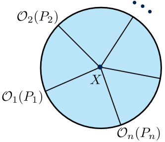
Figure 5: Witten diagram for a $n$-point contact interaction in AdS. The interior of the disk represents the bulk of AdS and the circumference represents its conformal boundary. The lines connecting the boundary points $P_{i}$ to the bulk point $X$ represent bulk to boundary propagators.

Witten diagrams

Consider the contact Witten diagram of figure 5. It corresponds to an interaction vertex $\lambda\phi_{1}\dots\phi_{n}$ in the bulk lagrangian and it contributes

$$\langle\mathcal{O}_{1}(P_{1})\dots\mathcal{O}_{n}(P_{n})\rangle=\lambda\int_{AdS}dX\prod_{i=1}^{n}\frac{\sqrt{\mathcal{C}_{\Delta_{i}}}}{(-2P_{i}\cdot X)^{\Delta_{i}}}$$ (179)

to the dual CFT correlation function. One can show that this corresponds to a constant Mellin amplitude,

$$M=\lambda\,\frac{1}{2}\pi^{\frac{d}{2}}\Gamma\left(\frac{\sum\Delta_{i}-d}{2}\right)\prod_{i=1}^{n}\frac{\sqrt{\mathcal{C}_{\Delta_{i}}}}{\Gamma(\Delta_{i})}\ .$$ (180)

Exercise 5.1

Check the last statement. Start by using the integral representation of the bulk to boundary propagators and performing the integral over AdS using Poincare coordinates as explained in exercise 3.5. This turns (179) into

$$\lambda\,\pi^{\frac{d}{2}}\Gamma\left(\frac{\sum\Delta_{i}-d}{2}\right)\int_{0}^{\infty}e^{-\sum_{i<j}s_{i}s_{j}P_{ij}}\prod_{i=1}^{n}\frac{\sqrt{\mathcal{C}_{\Delta_{i}}}}{\Gamma(\Delta_{i})}s_{i}^{\Delta_{i}-1}ds_{i}\ .$$ (181)

Next, use the Mellin representation ($c>0$)

$$e^{-s_{i}s_{j}P_{ij}}=\int_{c-i\infty}^{c+i\infty}\frac{d\gamma_{ij}}{2\pi i}\Gamma(\gamma_{ij})(s_{i}s_{j}P_{ij})^{-\gamma_{ij}}$$ (182)

for $n(n-3)/2$ exponential factors. A good choice is to keep $n$ factors, corresponding to the exponential

$$e^{-s_{1}\sum_{i=2}^{n}s_{i}P_{1i}-s_{2}s_{3}P_{23}}\,.$$ (183)

The integrals over $s_{4},\dots,s_{n}$ can be easily done in terms of $\Gamma$-functions. Finally, do the integrals over $s_{1},s_{2},s_{3}$ using the same type of change of variables as in exercise 3.5.

This result can be easily generalized to interaction vertices with derivatives. For example, the vertex $\lambda(\nabla_{\alpha}\phi_{1}\nabla^{\alpha}\phi_{2})\phi_{3}\dots\phi_{n}$ gives rise to

$$\langle\mathcal{O}_{1}(P_{1})\dots\mathcal{O}_{n}(P_{n})\rangle=\lambda\int_{AdS}dX\prod_{i=3}^{n}\frac{\sqrt{\mathcal{C}_{\Delta_{i}}}}{(-2P_{i}\cdot X)^{\Delta_{i}}}\times$$ (184)

$$\qquad\qquad\times(\eta^{AB}+X^{A}X^{B})\frac{\partial}{\partial X^{A}}\frac{\sqrt{\mathcal{C}_{\Delta_{1}}}}{(-2P_{1}\cdot X)^{\Delta_{1}}}\frac{\partial}{\partial X^{B}}\frac{\sqrt{\mathcal{C}_{\Delta_{2}}}}{(-2P_{2}\cdot X)^{\Delta_{2}}}\,.$$

Here we have used the fact that covariant derivatives in AdS can be computed as partial derivatives in the embedding space projected to the AdS sub-manifold. This gives

$$\lambda\Delta_{1}\Delta_{2}\left(-2P_{12}\,D_{\Delta_{1}+1,\Delta_{2}+1,\Delta_{3},\dots,\Delta_{n}}+D_{\Delta_{1},\Delta_{2},\Delta_{3},\dots,\Delta_{n}}\right)\prod_{i=1}^{n}\sqrt{\mathcal{C}_{\Delta_{i}}}$$ (185)

where we introduced the D-function [33]

$$D_{\Delta_{1},\dots,\Delta_{n}}\equiv\int_{AdS}dX\prod_{i=1}^{n}\frac{1}{(-2P_{i}\cdot X)^{\Delta_{i}}}\,.$$ (186)

More generally, it is clear that the contact Witten diagram associated with a generic vertex $\lambda\nabla\dots\nabla\phi_{1}\nabla\dots\nabla\phi_{2}\dots\nabla\dots\nabla\phi_{n}$ with all derivatives contracted among different fields, gives rise to a linear combination of terms of the form

$$D_{\Delta_{1}+\Lambda_{1},\dots,\Delta_{n}+\Lambda_{n}}\prod_{i<j}^{n}P_{ij}^{\lambda_{ij}}$$ (187)

where $\lambda_{ij}$ are non-negative integers and $\Lambda_{i}=\sum_{j\neq i}\lambda_{ij}$. As we will see in the next exercise, the Mellin amplitude of (187) is a polynomial in the Mellin variables. Therefore, the Mellin amplitude associated to contact Witten diagrams is polynomial. The absence of poles in the Mellin amplitude means that the conformal block decomposition of the contact diagram only contains multi-trace operators, in agreement with previous results [85, 86].

Exercise 5.2

If the vertex $\lambda\nabla\dots\nabla\phi_{1}\nabla\dots\nabla\phi_{2}\dots\nabla\dots\nabla\phi_{n}$ has $2N=2\sum_{i<j}\alpha_{ij}$ derivatives with $\alpha_{ij}$ contractions of derivatives acting on $\phi_{i}$ and $\phi_{j}$, show that the contact Witten diagram is given by

$$\lambda\left(\prod_{i=1}^{n}\sqrt{\mathcal{C}_{\Delta_{i}}}\right)D_{\Delta_{1}+\Lambda_{1},\dots,\Delta_{n}+\Lambda_{n}}\prod_{i<j}^{n}(-2P_{ij})^{\alpha_{ij}}+\dots$$ (188)

where $\Lambda_{i}=\sum_{j\neq i}\alpha_{ij}$ and the $\dots$ represent similar terms with less $P_{ij}$ factors. Hint: use the trick of writing covariant derivatives in AdS as partial derivatives in the embedding space projected to the AdS sub-manifold.

The Mellin representation of the $D$-functions is very simple. As we saw in exercise 5.1, the Mellin amplitude associated to $D_{\Delta_{1},\dots,\Delta_{n}}$ is simply

$$\frac{\pi^{\frac{d}{2}}\Gamma\left(\frac{\sum\Delta_{i}-d}{2}\right)}{2\prod_{i=1}^{n}\Gamma(\Delta_{i})}\ .$$ (189)

Show that the Mellin amplitude associated to the correlation function (188) is given by the polynomial

$$\lambda\left(\prod_{i=1}^{n}\sqrt{\mathcal{C}_{\Delta_{i}}}\right)\frac{\pi^{\frac{d}{2}}\Gamma\left(\frac{\sum\Delta_{i}+2N-d}{2}\right)}{2\prod_{i=1}^{n}\Gamma(\Delta_{i}+\Lambda_{i})}\prod_{i<j}^{n}(-2\gamma_{ij})^{\alpha_{ij}}+\dots$$ (190)

where the $\dots$ represent terms of lower degree in $\gamma_{ij}$. Hint: this follows easily from shifting the integration variables in the Mellin representation (157).

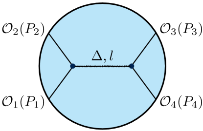
Figure 6: Witten diagram describing the exchange of a bulk field dual to an operator of dimension $\Delta$ and spin $l$.

Consider now the Witten diagram shown in figure 6 describing the exchange of a bulk field dual to a single-trace boundary operator $\mathcal{O}$ of dimension $\Delta$ and spin $l$. The conformal block decomposition of this diagram in the (12)(34) channel contains the single-trace operator $\mathcal{O}$ plus double-trace operators schematically of the form $\mathcal{O}_{1}(\partial^{2})^{n}\partial_{\mu_{1}\dots\mu_{j}}\mathcal{O}_{2}$ and $\mathcal{O}_{3}(\partial^{2})^{n}\partial_{\mu_{1}\dots\mu_{j}}\mathcal{O}_{4}$. Moreover, the OPE in the crossed channels only contains double-trace operators. This means that the Mellin amplitude is of the form

$$M=C_{12\mathcal{O}}C_{34\mathcal{O}}\sum_{m=0}^{\infty}\frac{Q_{l,m}(t)}{s-\Delta+l-2m}+R(s,t)$$ (191)

where the OPE coefficients $C_{12\mathcal{O}}$ and $C_{34\mathcal{O}}$ are proportional to the bulk cubic couplings and $R(s,t)$ is an analytic function. The residues are proportional to degree $l$ Mack polynomials $Q_{l,m}(t)$ which are entirely fixed by conformal symmetry as we saw in 2. If we choose minimal coupling between the spin $l$ bulk field and the external scalars, then $R(s,t)$ is a polynomial of degree $\leq l-1$. This is particularly simple in the case of a scalar exchange ($l=0$). Then the residues are independent of $t$ and $R=0$ [87]. Notice that this simple looking Mellin amplitude gives rise to a rather involved function of the cross-ratios in position space. This example illustrates clearly the advantage of using the Mellin reprsentation to describe Witten diagrams.

The Mellin amplitude of a general tree-level scalar Witten diagrams was determined in [88, 89, 90, 91]. The final result can be summarized in the following Feynman rules:

• Associate a momentum $p_{j}$ to every line (propagator) in the Witten diagram. External lines have incoming momentum $p_{i}$ satisfying $-p_{i}^{2}=\Delta_{i}$. Momentum is conserved at every vertex of the diagram.

• Assign an integer $m_{j}$ to every line. External lines have $m_{i}=0$.

• Every internal line (bulk-to-bulk propagator) contributes a factor

  $$\frac{S_{m_{j}}^{\Delta_{j}}}{p_{j}^{2}+\Delta_{j}+2m_{j}}$$ (193)

  where $\Delta_{j}$ is the dimension of the propagating scalar field.

• Every vertex, $g\phi_{1}\dots\phi_{k}$ joining $k$ lines, contributes a factor

  $$g\,V^{\Delta_{1}\dots\Delta_{k}}_{m_{1}\dots m_{k}}$$ (194)

• Sum over all integers $m_{j}$ associated with internal lines. Each sum runs from 0 to $\infty$.

• Multiply by

  $$\mathcal{N}=\frac{\pi^{\frac{d}{2}}}{2}\prod_{i=1}^{n}\frac{\sqrt{\mathcal{C}_{\Delta_{i}}}}{\Gamma(\Delta_{i})}$$ (195)

  to get the $n$-point Mellin amplitude in our normalization of the external operators.

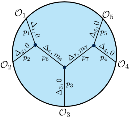
Figure 7: A tree level scalar Witten diagram contributing to a 5-point function. The auxiliary momenta $p_{i}$ is conserved at each vertex, i.e. $p_{6}=p_{1}+p_{2}$ and $p_{7}=p_{4}+p_{5}$.

As an example, the Witten diagram in figure 7 gives rise to the following Mellin amplitude

$$\mathcal{N}\sum_{m_{6}=0}^{\infty}\sum_{m_{7}=0}^{\infty}V^{\Delta_{1}\Delta_{2}\Delta_{6}}_{0\,0\,m_{6}}\frac{S_{m_{6}}^{\Delta_{6}}}{p_{6}^{2}+\Delta_{6}+2m_{6}}V^{\Delta_{6}\Delta_{3}\Delta_{7}}_{m_{6}\,0\,m_{7}}\frac{S_{m_{7}}^{\Delta_{7}}}{p_{7}^{2}+\Delta_{7}+2m_{7}}V^{\Delta_{7}\Delta_{4}\Delta_{5}}_{m_{7}\,0\,0}$$

where $p_{6}^{2}=(p_{1}+p_{2})^{2}=2\gamma_{12}-\Delta_{1}-\Delta_{2}$ and $p_{7}^{2}=(p_{4}+p_{5})^{2}=2\gamma_{45}-\Delta_{4}-\Delta_{5}$. These Feynman rules suggest that we should think of the Mellin amplitude as an amputated amplitude because the bulk to boundary propagators do not contribute. In the case of scalar tree level diagrams (with non-derivative interaction vertices), the only dependence in the Mellin variables $\gamma_{ij}$ comes from the bulk-to-bulk propagators. It is not known how to generalize these Feynman rules for loop diagrams or tree-level diagrams involving fields with spin. There are partial results in literature [89, 83] but nothing systematic. Mellin amplitudes are also useful in the context of weakly coupled CFTs. The associated Feynman rules for tree level diagrams were given in [92].

Exercise 5.3

Consider the residue of the Mellin amplitude at the first pole ($m=0$) associated to a bulk-to-bulk propagator. Show that the Feynman rules above are compatible with the factorization property (176) of this residue. Extra: check the factorization formula (177) for the satellite poles with $m>0$.

Flat space limit of AdS

If we consider a scattering process where all length scales are much smaller than the AdS radius $R$ then the curvature effects should be negligible. Consider a relativistic invariant theory in flat spacetime with a characteristic length scale $\ell_{s}$ (this scale could come from a mass or from a dimensionful coupling). Then, a scattering amplitude $\mathcal{T}_{n}$ of $n$ massless scalar particles in this theory will depend on $\ell_{s}$ and on the relativistic invariants $k_{i}\cdot k_{j}$, where $k_{i}$ are the momenta of the external particles. On the other hand, this theory in AdS will give rise to Mellin amplitudes that depend on the dimensionless parameter $\theta=R/\ell_{s}$ and the Mellin variables $\gamma_{ij}$. We claim that these two quantities are related by

$$\frac{\mathcal{T}_{n}(\ell_{s},k_{i})}{\ell_{s}^{n\frac{d-1}{2}-d-1}}=\lim_{\theta\to\infty}\frac{1}{\mathcal{N}}\int_{\Gamma}\frac{d\alpha}{2\pi i}\alpha^{\frac{d-\sum\Delta_{i}}{2}}e^{\alpha}\frac{M_{n}\left(\theta,\gamma_{ij}=\frac{\theta^{2}}{2\alpha}\ell_{s}^{2}\,k_{i}\cdot k_{j}\right)}{\theta^{n\frac{1-d}{2}+d+1}}$$ (196)

where the contour $\Gamma$ runs parallel to the imaginary axis and passes to the right of the branch point at $\alpha=0$ and to the left of all poles of $M_{n}$. The powers of $\ell_{s}$ where introduced to make both sides of the equation dimensionless and the constant $\mathcal{N}$ was given in (195). The external particles are massless in flat space but in AdS they can have any scaling dimension $\Delta_{i}$ of order 1. We expect this equation to hold when both sides of the equation are well defined. In case the flat space scattering amplitude $\mathcal{T}_{n}$ is IR divergent, we expect that the limit $\theta\to\infty$ of the Mellin amplitude will not be finite.

Exercise 5.4

Consider the vertex $\lambda\nabla\dots\nabla\phi_{1}\dots\nabla\dots\nabla\phi_{n}$ discussed in exercise 5.2 in $d+1$ spacetime dimensions. Start by writing the coupling constant $\lambda$ as a power $(\ell_{s})^{q}$ of a characteristic length scale $\ell_{s}$ and determine the value of $q$. Then, use the Mellin amplitude (190) in the flat space limit formula (196) and obtain the expected $n$-particle scattering amplitude

$$\mathcal{T}_{n}=\lambda\prod_{i<j}(-k_{i}\cdot k_{j})^{\alpha_{ij}}\ .$$ (197)

The last exercise can be seen as a derivation of the flat space limit formula (196). The point is that a generic Feynman diagram can be written as a (infinite) sum of contact diagrams with any number of derivatives. This corresponds to integrating out the internal particles and replacing there effect by contact vertices among the external particles. Since formula (196) works for any contact diagram it should work in general. This has been tested in several explicit examples, including 1-loop diagrams [87, 88, 93]. In addition, the same formula was derived in [90] using a wave-packet construction where the scattering region was limited to a small flat region of AdS.

In principle, formula (196) provides a non-perturbative definition of string theory scattering amplitudes in terms of SYM correlation functions. However, we do not know how to directly compute SYM correlators at strong coupling. In practice, what we can do is to use formula (196) in the opposite direction, i.e. we can use known string scattering amplitudes in flat space to obtain information about the strong coupling expansion of SYM correlators [87, 94]. If the external particles are massive in flat space then formula (196) is not adequate. This case was studied in [95].

4 Open questions

The study of Mellin amplitudes is still very incomplete. Firstly, it is important to understand in what conditions do we have a well defined analytic Mellin amplitude. For example, in free CFTs the Mellin representation requires some form of regularization. This might be a technical detail but it would be useful to understand in general the status of the Mellin representation. Another important question is the asymptotic behavior of the Mellin amplitude when the Mellin variables are large. In the case of the four-point Mellin amplitude discussed in 2, the limit of large $s$ with fixed $t$ is called the Regge limit in analogy with flat space scattering amplitudes. In [96], we studied this limit using Regge theory techniques and making some reasonable assumptions about the large spin behaviour of the conformal partial amplitudes. Proving these assumptions is an important open question. The bound on chaos [97] is another possible approach to the Regge limit of Mellin amplitudes. Notice that if we can tame the asymptotic behaviour of $M(s,t)$ when $s\to\infty$, then we can write a dispersion relation that expresses $M(s,t)$ in terms of its poles in $s$, which are given by (173). This could provide a reformulation of the conformal bootstrap approach.

In the holographic context, it would be interesting to establish more general Feynman rules for Mellin amplitudes associated to Witten diagrams involving loops and particles with spin. It would also be useful to generalize more modern approaches to scattering amplitudes, like BCFW [98] or CHY [99], to Mellin amplitudes.

Acknowledgements

I would like to thank the students of TASI 2015 for their questions and enthusiasm. I am also grateful to the organizers Joe Polchinski, Pedro Vieira, Tom DeGrand and Oliver DeWolfe for their invitation and their patience with my delays in finishing these notes. Centro de Física do Porto is partially funded by FCT. The research leading to these results has received funding from the People Programme (Marie Curie Actions) of the European Union’s Seventh Framework Programme FP7/2007-2013/ under REA Grant Agreement No 317089 and CERN/FIS-NUC/0045/2015.

References

- [1] J. M. Maldacena, “The Large N limit of superconformal field theories and supergravity,” Int.J.Theor.Phys. 38 (1999) 1113–1133, arXiv:hep-th/9711200 [hep-th].
- [2] S. S. Gubser, I. R. Klebanov, and A. M. Polyakov, “Gauge theory correlators from noncritical string theory,” Phys. Lett. B428 (1998) 105–114, arXiv:hep-th/9802109 [hep-th].
- [3] E. Witten, “Anti-de Sitter space and holography,” Adv. Theor. Math. Phys. 2 (1998) 253–291, arXiv:hep-th/9802150 [hep-th].
- [4] A. Almheiri, D. Marolf, J. Polchinski, and J. Sully, “Black Holes: Complementarity or Firewalls?,” JHEP 02 (2013) 062, arXiv:1207.3123 [hep-th].
- [5] D. Simmons-Duffin, “TASI Lectures on the Conformal Bootstrap,” arXiv:1602.07982 [hep-th].
- [6] S. Rychkov, “EPFL Lectures on Conformal Field Theory in Dimensions,” arXiv:1601.05000 [hep-th].
- [7] J. D. Qualls, “Lectures on Conformal Field Theory,” arXiv:1511.04074 [hep-th].
- [8] O. Aharony, S. S. Gubser, J. M. Maldacena, H. Ooguri, and Y. Oz, “Large N field theories, string theory and gravity,” Phys. Rept. 323 (2000) 183–386, arXiv:hep-th/9905111 [hep-th].
- [9] J. McGreevy, “Holographic duality with a view toward many-body physics,” Adv. High Energy Phys. 2010 (2010) 723105, arXiv:0909.0518 [hep-th].
- [10] E. D’Hoker and D. Z. Freedman, “Supersymmetric gauge theories and the AdS / CFT correspondence,” arXiv:hep-th/0201253 [hep-th].
- [11] D. Mateos, “String Theory and Quantum Chromodynamics,” Class. Quant. Grav. 24 (2007) S713–S740, arXiv:0709.1523 [hep-th].
- [12] H. Nastase, “Introduction to AdS-CFT,” arXiv:0712.0689 [hep-th].
- [13] S. S. Gubser and A. Karch, “From gauge-string duality to strong interactions: A Pedestrian’s Guide,” Ann. Rev. Nucl. Part. Sci. 59 (2009) 145–168, arXiv:0901.0935 [hep-th].
- [14] S. A. Hartnoll, “Lectures on holographic methods for condensed matter physics,” Class. Quant. Grav. 26 (2009) 224002, arXiv:0903.3246 [hep-th].
- [15] J. Polchinski, “Introduction to Gauge/Gravity Duality,” arXiv:1010.6134 [hep-th].
- [16] S. A. Hartnoll, “Horizons, holography and condensed matter,” arXiv:1106.4324 [hep-th].
- [17] J. Kaplan, “Lectures on AdS/CFT from the Bottom Up.” http://www.pha.jhu.edu/~jaredk/AdSCFTCourseNotesPublic.pdf.
- [18] P. A. M. Dirac, “Wave equations in conformal space,” Annals Math. 37 (1936) 429–442.
- [19] G. Mack and A. Salam, “Finite component field representations of the conformal group,” Annals Phys. 53 (1969) 174–202.
- [20] D. G. Boulware, L. S. Brown, and R. D. Peccei, “Deep-inelastic electroproduction and conformal symmetry,” Phys. Rev. D2 (1970) 293–298.
- [21] S. Ferrara, R. Gatto, and A. F. Grillo, “Conformal algebra in space-time and operator product expansion,” Springer Tracts Mod. Phys. 67 (1973) 1–64.
- [22] S. Ferrara, A. F. Grillo, and R. Gatto, “Tensor representations of conformal algebra and conformally covariant operator product expansion,” Annals Phys. 76 (1973) 161–188.
- [23] L. Cornalba, M. S. Costa, and J. Penedones, “Deep Inelastic Scattering in Conformal QCD,” JHEP 03 (2010) 133, arXiv:0911.0043 [hep-th].
- [24] S. Weinberg, “Six-dimensional Methods for Four-dimensional Conformal Field Theories,” Phys. Rev. D82 (2010) 045031, arXiv:1006.3480 [hep-th].
- [25] M. S. Costa, J. Penedones, D. Poland, and S. Rychkov, “Spinning Conformal Correlators,” JHEP 11 (2011) 071, arXiv:1107.3554 [hep-th].
- [26] G. ’t Hooft, “A Planar Diagram Theory for Strong Interactions,” Nucl.Phys. B72 (1974) 461.
- [27] E. Witten, “Baryons in the 1/n Expansion,” Nucl. Phys. B160 (1979) 57–115.
- [28] F. A. Dolan and H. Osborn, “Conformal four point functions and the operator product expansion,” Nucl. Phys. B599 (2001) 459–496, arXiv:hep-th/0011040 [hep-th].
- [29] S. El-Showk and K. Papadodimas, “Emergent Spacetime and Holographic CFTs,” JHEP 10 (2012) 106, arXiv:1101.4163 [hep-th].
- [30] H. Liu and A. A. Tseytlin, “D = 4 superYang-Mills, D = 5 gauged supergravity, and D = 4 conformal supergravity,” Nucl. Phys. B533 (1998) 88–108, arXiv:hep-th/9804083 [hep-th].
- [31] H. Liu and A. A. Tseytlin, “On four point functions in the CFT / AdS correspondence,” Phys. Rev. D59 (1999) 086002, arXiv:hep-th/9807097 [hep-th].
- [32] E. D’Hoker, D. Z. Freedman, S. D. Mathur, A. Matusis, and L. Rastelli, “Graviton and gauge boson propagators in AdS(d+1),” Nucl. Phys. B562 (1999) 330–352, arXiv:hep-th/9902042 [hep-th].
- [33] E. D’Hoker, D. Z. Freedman, S. D. Mathur, A. Matusis, and L. Rastelli, “Graviton exchange and complete four point functions in the AdS / CFT correspondence,” Nucl. Phys. B562 (1999) 353–394, arXiv:hep-th/9903196 [hep-th].
- [34] M. S. Costa, V. Gonçalves, and J. Penedones, “Spinning AdS Propagators,” JHEP 09 (2014) 064, arXiv:1404.5625 [hep-th].
- [35] V. Balasubramanian and P. Kraus, “A Stress tensor for Anti-de Sitter gravity,” Commun. Math. Phys. 208 (1999) 413–428, arXiv:hep-th/9902121 [hep-th].
- [36] K. Skenderis, “Lecture notes on holographic renormalization,” Class. Quant. Grav. 19 (2002) 5849–5876, arXiv:hep-th/0209067 [hep-th].
- [37] H. Osborn and A. C. Petkou, “Implications of conformal invariance in field theories for general dimensions,” Annals Phys. 231 (1994) 311–362, arXiv:hep-th/9307010 [hep-th].
- [38] I. Heemskerk, J. Penedones, J. Polchinski, and J. Sully, “Holography from Conformal Field Theory,” JHEP 10 (2009) 079, arXiv:0907.0151 [hep-th].
- [39] X. O. Camanho, J. D. Edelstein, J. Maldacena, and A. Zhiboedov, “Causality Constraints on Corrections to the Graviton Three-Point Coupling,” JHEP 02 (2016) 020, arXiv:1407.5597 [hep-th].
- [40] N. Arkani-Hamed, F. Cachazo, and J. Kaplan, “What is the Simplest Quantum Field Theory?,” JHEP 09 (2010) 016, arXiv:0808.1446 [hep-th].
- [41] N. Beisert et al., “Review of AdS/CFT Integrability: An Overview,” Lett. Math. Phys. 99 (2012) 3–32, arXiv:1012.3982 [hep-th].
- [42] S. Lee, S. Minwalla, M. Rangamani, and N. Seiberg, “Three point functions of chiral operators in D = 4, N=4 SYM at large N,” Adv. Theor. Math. Phys. 2 (1998) 697–718, arXiv:hep-th/9806074 [hep-th].
- [43] V. Pestun, “Localization of gauge theory on a four-sphere and supersymmetric Wilson loops,” Commun. Math. Phys. 313 (2012) 71–129, arXiv:0712.2824 [hep-th].
- [44] J. K. Erickson, G. W. Semenoff, and K. Zarembo, “Wilson loops in N=4 supersymmetric Yang-Mills theory,” Nucl. Phys. B582 (2000) 155–175, arXiv:hep-th/0003055 [hep-th].
- [45] N. Gromov, V. Kazakov, and P. Vieira, “Exact Spectrum of Planar Supersymmetric Yang-Mills Theory: Konishi Dimension at Any Coupling,” Phys. Rev. Lett. 104 (2010) 211601, arXiv:0906.4240 [hep-th].
- [46] B. Basso, A. Sever, and P. Vieira, “Spacetime and Flux Tube S-Matrices at Finite Coupling for N=4 Supersymmetric Yang-Mills Theory,” Phys. Rev. Lett. 111 no. 9, (2013) 091602, arXiv:1303.1396 [hep-th].
- [47] B. Basso, S. Komatsu, and P. Vieira, “Structure Constants and Integrable Bootstrap in Planar N=4 SYM Theory,” arXiv:1505.06745 [hep-th].
- [48] T. Banks, W. Fischler, S. H. Shenker, and L. Susskind, “M theory as a matrix model: A Conjecture,” Phys. Rev. D55 (1997) 5112–5128, arXiv:hep-th/9610043 [hep-th].
- [49] S. Catterall and T. Wiseman, “Towards lattice simulation of the gauge theory duals to black holes and hot strings,” JHEP 12 (2007) 104, arXiv:0706.3518 [hep-lat].
- [50] K. N. Anagnostopoulos, M. Hanada, J. Nishimura, and S. Takeuchi, “Monte Carlo studies of supersymmetric matrix quantum mechanics with sixteen supercharges at finite temperature,” Phys. Rev. Lett. 100 (2008) 021601, arXiv:0707.4454 [hep-th].
- [51] S. Catterall and T. Wiseman, “Black hole thermodynamics from simulations of lattice Yang-Mills theory,” Phys. Rev. D78 (2008) 041502, arXiv:0803.4273 [hep-th].
- [52] M. Hanada, Y. Hyakutake, J. Nishimura, and S. Takeuchi, “Higher derivative corrections to black hole thermodynamics from supersymmetric matrix quantum mechanics,” Phys. Rev. Lett. 102 (2009) 191602, arXiv:0811.3102 [hep-th].
- [53] S. Catterall and T. Wiseman, “Extracting black hole physics from the lattice,” JHEP 04 (2010) 077, arXiv:0909.4947 [hep-th].
- [54] M. Hanada, J. Nishimura, Y. Sekino, and T. Yoneya, “Direct test of the gauge-gravity correspondence for Matrix theory correlation functions,” JHEP 12 (2011) 020, arXiv:1108.5153 [hep-th].
- [55] M. Hanada, Y. Hyakutake, G. Ishiki, and J. Nishimura, “Holographic description of quantum black hole on a computer,” Science 344 (2014) 882–885, arXiv:1311.5607 [hep-th].
- [56] J. Polchinski and E. Silverstein, “Dual Purpose Landscaping Tools: Small Extra Dimensions in AdS/CFT,” arXiv:0908.0756 [hep-th].
- [57] S. de Alwis, R. K. Gupta, F. Quevedo, and R. Valandro, “On KKLT/CFT and LVS/CFT Dualities,” JHEP 07 (2015) 036, arXiv:1412.6999 [hep-th].
- [58] I. R. Klebanov and A. M. Polyakov, “AdS dual of the critical O(N) vector model,” Phys. Lett. B550 (2002) 213–219, arXiv:hep-th/0210114 [hep-th].
- [59] E. Sezgin and P. Sundell, “Massless higher spins and holography,” Nucl. Phys. B644 (2002) 303–370, arXiv:hep-th/0205131 [hep-th]. [Erratum: Nucl. Phys.B660,403(2003)].
- [60] S. Giombi, S. Minwalla, S. Prakash, S. P. Trivedi, S. R. Wadia, and X. Yin, “Chern-Simons Theory with Vector Fermion Matter,” Eur. Phys. J. C72 (2012) 2112, arXiv:1110.4386 [hep-th].
- [61] O. Aharony, G. Gur-Ari, and R. Yacoby, “Correlation Functions of Large N Chern-Simons-Matter Theories and Bosonization in Three Dimensions,” JHEP 12 (2012) 028, arXiv:1207.4593 [hep-th].
- [62] M. R. Gaberdiel and R. Gopakumar, “Minimal Model Holography,” J. Phys. A46 (2013) 214002, arXiv:1207.6697 [hep-th].
- [63] P. Kovtun and A. Ritz, “Black holes and universality classes of critical points,” Phys. Rev. Lett. 100 (2008) 171606, arXiv:0801.2785 [hep-th].
- [64] S. W. Hawking and D. N. Page, “Thermodynamics of Black Holes in anti-De Sitter Space,” Commun. Math. Phys. 87 (1983) 577.
- [65] S. Ryu and T. Takayanagi, “Holographic derivation of entanglement entropy from AdS/CFT,” Phys. Rev. Lett. 96 (2006) 181602, arXiv:hep-th/0603001 [hep-th].
- [66] J. M. Maldacena, “Wilson loops in large N field theories,” Phys. Rev. Lett. 80 (1998) 4859–4862, arXiv:hep-th/9803002 [hep-th].
- [67] P. Romatschke and U. Romatschke, “Viscosity Information from Relativistic Nuclear Collisions: How Perfect is the Fluid Observed at RHIC?,” Phys. Rev. Lett. 99 (2007) 172301, arXiv:0706.1522 [nucl-th].
- [68] A. B. Zamolodchikov, “Irreversibility of the Flux of the Renormalization Group in a 2D Field Theory,” JETP Lett. 43 (1986) 730–732. [Pisma Zh. Eksp. Teor. Fiz.43,565(1986)].
- [69] R. C. Myers and A. Sinha, “Holographic c-theorems in arbitrary dimensions,” JHEP 01 (2011) 125, arXiv:1011.5819 [hep-th].
- [70] Z. Komargodski and A. Schwimmer, “On Renormalization Group Flows in Four Dimensions,” JHEP 12 (2011) 099, arXiv:1107.3987 [hep-th].
- [71] H. Casini and M. Huerta, “On the RG running of the entanglement entropy of a circle,” Phys. Rev. D85 (2012) 125016, arXiv:1202.5650 [hep-th].
- [72] D. M. Hofman and J. Maldacena, “Conformal collider physics: Energy and charge correlations,” JHEP 05 (2008) 012, arXiv:0803.1467 [hep-th].
- [73] D. M. Hofman, D. Li, D. Meltzer, D. Poland, and F. Rejon-Barrera, “A Proof of the Conformal Collider Bounds,” JHEP 06 (2016) 111, arXiv:1603.03771 [hep-th].
- [74] T. Faulkner, R. G. Leigh, O. Parrikar, and H. Wang, “Modular Hamiltonians for Deformed Half-Spaces and the Averaged Null Energy Condition,” arXiv:1605.08072 [hep-th].
- [75] A. L. Fitzpatrick, J. Kaplan, D. Poland, and D. Simmons-Duffin, “The Analytic Bootstrap and AdS Superhorizon Locality,” JHEP 12 (2013) 004, arXiv:1212.3616 [hep-th].
- [76] Z. Komargodski and A. Zhiboedov, “Convexity and Liberation at Large Spin,” JHEP 11 (2013) 140, arXiv:1212.4103 [hep-th].
- [77] A. Kaviraj, K. Sen, and A. Sinha, “Analytic bootstrap at large spin,” JHEP 11 (2015) 083, arXiv:1502.01437 [hep-th].
- [78] A. Kaviraj, K. Sen, and A. Sinha, “Universal anomalous dimensions at large spin and large twist,” JHEP 07 (2015) 026, arXiv:1504.00772 [hep-th].
- [79] G. Mack, “D-independent representation of Conformal Field Theories in D dimensions via transformation to auxiliary Dual Resonance Models. Scalar amplitudes,” arXiv:0907.2407 [hep-th].
- [80] G. Mack, “D-dimensional Conformal Field Theories with anomalous dimensions as Dual Resonance Models,” Bulg. J. Phys. 36 (2009) 214–226, arXiv:0909.1024 [hep-th].
- [81] K. Symanzik, “On Calculations in conformal invariant field theories,” Lett. Nuovo Cim. 3 (1972) 734–738.
- [82] V. K. Dobrev, V. B. Petkova, S. G. Petrova, and I. T. Todorov, “Dynamical Derivation of Vacuum Operator Product Expansion in Euclidean Conformal Quantum Field Theory,” Phys. Rev. D13 (1976) 887.
- [83] V. Gonçalves, J. Penedones, and E. Trevisani, “Factorization of Mellin amplitudes,” JHEP 10 (2015) 040, arXiv:1410.4185 [hep-th].
- [84] M. S. Costa, T. Hansen, J. Penedones, and E. Trevisani, “Projectors and seed conformal blocks for traceless mixed-symmetry tensors,” JHEP 07 (2016) 018, arXiv:1603.05551 [hep-th].
- [85] H. Liu, “Scattering in anti-de Sitter space and operator product expansion,” Phys. Rev. D60 (1999) 106005, arXiv:hep-th/9811152 [hep-th].
- [86] E. D’Hoker and D. Z. Freedman, “General scalar exchange in AdS(d+1),” Nucl. Phys. B550 (1999) 261–288, arXiv:hep-th/9811257 [hep-th].
- [87] J. Penedones, “Writing CFT correlation functions as AdS scattering amplitudes,” JHEP 03 (2011) 025, arXiv:1011.1485 [hep-th].
- [88] A. L. Fitzpatrick, J. Kaplan, J. Penedones, S. Raju, and B. C. van Rees, “A Natural Language for AdS/CFT Correlators,” JHEP 11 (2011) 095, arXiv:1107.1499 [hep-th].
- [89] M. F. Paulos, “Towards Feynman rules for Mellin amplitudes,” JHEP 10 (2011) 074, arXiv:1107.1504 [hep-th].
- [90] A. L. Fitzpatrick and J. Kaplan, “Analyticity and the Holographic S-Matrix,” JHEP 10 (2012) 127, arXiv:1111.6972 [hep-th].
- [91] D. Nandan, A. Volovich, and C. Wen, “On Feynman Rules for Mellin Amplitudes in AdS/CFT,” JHEP 05 (2012) 129, arXiv:1112.0305 [hep-th].
- [92] A. A. Nizami, A. Rudra, S. Sarkar, and M. Verma, “Exploring Perturbative Conformal Field Theory in Mellin space,” arXiv:1607.07334 [hep-th].
- [93] A. L. Fitzpatrick and J. Kaplan, “Unitarity and the Holographic S-Matrix,” JHEP 10 (2012) 032, arXiv:1112.4845 [hep-th].
- [94] V. Gonçalves, “Four point function of stress-tensor multiplet at strong coupling,” JHEP 04 (2015) 150, arXiv:1411.1675 [hep-th].
- [95] M. F. Paulos, J. Penedones, J. Toledo, B. C. van Rees, and P. Vieira, “The S-matrix Bootstrap I: QFT in AdS,” arXiv:1607.06109 [hep-th].
- [96] M. S. Costa, V. Goncalves, and J. Penedones, “Conformal Regge theory,” JHEP 12 (2012) 091, arXiv:1209.4355 [hep-th].
- [97] J. Maldacena, S. H. Shenker, and D. Stanford, “A bound on chaos,” arXiv:1503.01409 [hep-th].
- [98] R. Britto, F. Cachazo, B. Feng, and E. Witten, “Direct proof of tree-level recursion relation in Yang-Mills theory,” Phys. Rev. Lett. 94 (2005) 181602, arXiv:hep-th/0501052 [hep-th].
- [99] F. Cachazo, S. He, and E. Y. Yuan, “Scattering of Massless Particles in Arbitrary Dimensions,” Phys. Rev. Lett. 113 no. 17, (2014) 171601, arXiv:1307.2199 [hep-th].