Abstract

The issue of electroweak vacuum stability is studied in presence of a scalar field which participates in modifying the minimal chaotic inflation model. It is shown that the threshold effect on the Higgs quartic coupling originating from the Higgs-inflaton sector interaction can essentially make the electroweak vacuum stable upto the Planck scale. On the other hand we observe that the new physics parameters in this combined framework are enough to provide deviation from the minimal chaotic inflation predictions so as to keep it consistent with recent observation by Planck 2015.

The discovery of the Higgs boson[1, 2, 3, 4] undoubtedly establishes the credibility of the Standard Model (SM) as a successful theory of fundamental interactions in nature. While the Higgs boson was the only particle in the SM that remained to be discovered until recently, its finding does not necessarily indicate the end for the hunt of particle physics. On the contrary, the discovery opens up several questions regarding the Higgs sector (or Higgs potential) of the SM. In particular the study of the Higgs potential turns out to be quite intriguing in view of the fact that the Higgs quartic coupling $\lambda_{h}$ becomes negative at high energies (the SM instability scale $\Lambda_{I}^{\textrm{SM}}\sim 10^{10}$ GeV) indicating a possible instability of the electroweak (EW) vacuum, as beyond $\Lambda_{I}^{\textrm{SM}}$ the Higgs potential becomes unbounded from below or it might have another minimum (a true minimum) at a very large field value[5, 6]. This poses (the latter possibility) a cosmological problem: why the early universe should favor the EW minimum in presence of a deeper one (the true minimum) at a large field value?

The vacuum stability problem of the Higgs potential is intensely tied up with the precise value of the top quark mass $m_{t}$[7, 8]. For a certain range of SM Higgs mass ($m_{h}$) and $m_{t}$, the problem is bit alleviated provided the lifetime of the EW vacuum exceeds the age of the Universe or in other words the EW vacuum becomes metastable. The current avilable data suggests the EW vacuum as a metastable one[11, 10, 9]. However the resolution exclusively depends on the precise measurement of $m_{t}$ that may push it to the instability region. One of the possible solutions is to introduce new physics in-between EW scale and $\Lambda_{I}^{\textrm{SM}}$. In view of SM’s incompetence to resolve some of the issues like dark matter, matter-antimatter asymmetry, neutrino mass and mixings, inflation etc, the introduction of new physics is of course a welcome feature.

In this work, we want to study how the vacuum stability problem gets affected in presence of inflation sector in the early universe. Successful inflation in early universe is required for structure formation. The inflationary predictions should however be consistent with Planck 2015[12] data. During inflation the Higgs field is expected to receive a typical fluctuation with amplitude of $\mathcal{O}(H_{\textrm{Inf}})$ where $H_{\textrm{Inf}}$ is the Hubble scale during inflation. So there is a possibility that it can be driven from the EW vacuum toward the unstable part of the Higgs potential provided $H_{\textrm{Inf}}>\Lambda_{I}^{\textrm{SM}}$ which is satisfied by most of the large field inflation models[13]. Now if the effective mass of the Higgs boson can be made sufficiently large during inflation ($m_{h}^{\textrm{eff}}>H_{\textrm{Inf}}$), the Higgs field will naturally evolve to origin and the problem can be evaded. This large effective mass term can be generated through Higgs-inflaton interaction as suggested in [14] and the dangerous effect on Higgs vacuum stability during inflation could be avoided. So an involvement of new physics (a scalar field involved in inflation) is required which can ensure Higgs field to remain at origin during inflationary period of the universe. Once the inflation is over, this field can then fall in the EW minimum as this minimum is close to the origin.

Concerning the model of inflation, the chaotic inflation[15] with quadratic potential is perhaps the simplest scenario. However it is in the verge of being excluded by the Planck 2015 observations[12]. Several ways are there to save this model [16, 17, 18, 19, 20, 21, 23, 22]. Idea behind all these is however common. If we can flatten the choatic potential dynamically, it can predict correct value of spectral index ($n_{s}$) and scalar to tensor ratio ($r$). One particular approach[16] seems interesting in this context where involvement of a second SM singlet scalar field (apart from the one responsible for chaotic inflation) is assumed. The effect of this additional scalar is to modify the quadratic potential $V_{\phi}$ to some extent.

Here we investigate the possibility of using this extra scalar field of the inflation system to take part in resolving the Higgs vacuum stability problem. It is shown in [24, 25] that involvement of a scalar field can indeed modify the stability condition of electroweak vacuum in SM provided this singlet field acquires a large vacuum expectation value. The threshold effect provides a tree level shift in $\lambda_{h}$ at a scale below which this heavy scalar would be integrated out. This turns out to be very effective in keeping the Higgs quartic coupling positive upto the scale $M_{P}$.

Previously, connecting the inflaton and the Higgs sector to solve the vacuum stability problem has been extensively studied in [26]. They have considered hilltop and quartic inflations where inflaton ($\phi$) itself plays the role of this singlet as at the end of inflation $\phi$ field gets a large vev. Below its mass scale the inflaton can be integrated out and the higgs quartic coupling gets a shift. The energy scale where this threshold effect occurs is therefore fixed by the inflaton mass $m$. Our approach however differs from [26]. We employ the chaotic inflation with potential $V_{\phi}=m^{2}\phi^{2}/2$ where $\langle\phi\rangle=0$ at the end of inflation. Following [16] another scalar field $\chi$ is introduced where its coupling with $\phi$ provides the required modification so that the inflationary predictions fall within the allowed $n_{s}-r$ region by Planck 2015[12]. In addition we suggest a modification where the $\chi$ field has a large vev ($v_{\chi}$) at its true minimum. It is found that the size of the vev is essentially unconstrained from inflation data. On the other hand this field can play important role in studying the Higgs vacuum stability issue. Apart from inflation, moduli fields[27] and the scalar singlet(s) involved in dark matter [29, 30, 33, 34, 35, 28, 31, 32], neutrinos [37, 38, 40, 41, 42, 43, 46, 47, 48, 45, 44, 39, 36] can have effect on the Higgs vacuum stability in many different ways.

We start by summarizing the features of the chaotic inflation with quadratic potential,

$$V_{\phi}=\frac{1}{2}m^{2}\phi^{2},$$ (1)

where the inflaton $\phi$ is a real scalar field (SM singlet) and $m$ is the mass parameter. With this potential, the slow roll happens at a super-Planckian value of the inflaton field $\phi$. The magnitude of $m$ is found to be $m\simeq 1.4\times 10^{13}$ GeV in order to be consistent with the observed amount of curvature perturbation. This potential yields the magnitude of spectral index $(n_{s})$ and tensor to scalar ratio ($r$) as $n_{s}=1-\frac{2}{N_{e}}\simeq 0.967$ and $r=\frac{8}{N_{e}}\simeq 0.133$ where the number of $e$-folds $(N_{e})$ is considered to be 60. However from observational point of view, Planck 2015[12] provides an upper-bound on $r\leq 0.11$ which seems to disfavor this minimal model for its prediction of large $r$. So a modification is highly appreciated to revive the model.

Following the recent proposal in [16], we consider a variant of the above potential

$$V_{\rm{I}}=\frac{1}{2}m^{2}\phi^{2}-\frac{c_{1}}{2}\phi^{2}(\chi^{2}-v_{\chi}^{2})+\frac{\lambda_{\chi}}{4}(\chi^{2}-v_{\chi}^{2})^{2},$$ (2)

where $m,c_{1},\lambda_{\chi}$ and $v_{\chi}$ are real and positive parameters. $\chi$ is another SM singlet scalar field which helps flattening the quadratic part of the potential involving $\phi$. We assume a $Z_{2}$ symmetry under which $\phi$ and $\chi$ fields are odd and hence they appear quadratically in the potential. The vev of the $\chi$ field in its global minimum is $v_{\chi}$. As it will turn out $v_{\chi}$ does not have almost any impact on the inflationary predictions. Note that we have not considered the higher order terms involving $\phi$, $e.g.\leavevmode\nobreak\ \phi^{4}$. The effect of those terms would be destructive in terms of the flatness of the potential. Therefore coefficients associated with those higher order terms in $\phi$ are assumed to be negligibly small.

Similar to the original chaotic inflation model with $V_{\phi}$, here also during inflation the $\phi$ field takes super-Planckian value. The potential is such that the $\chi$ field receives a negative mass-squared term which depends on the field value of $\phi$. Therefore $\chi$ acquires a large field value due to its coupling (through $c_{1}$ term) with the $\phi$ field

$$\langle\chi\rangle=\Big{(}v_{\chi}^{2}+\frac{c_{1}}{\lambda_{\chi}}\phi^{2}\Big{)}^{1/2}\simeq\sqrt{\frac{c_{1}}{\lambda_{\chi}}}\phi=\chi_{\textrm{I}},$$ (3)

$\chi_{\textrm{I}}$ is however considered to be sub-Planckian which implies $\frac{c_{1}}{\lambda_{\chi}}\ll 1$. Once $\phi$ rolls down to a smaller value, $\langle\chi\rangle$ decreases. When $\phi$ finally settles at origin, $\langle\chi\rangle$ is shifted to its minimum $v_{\chi}$. The magnitude of $v_{\chi}$ is assumed to be below $m$ $(v_{\chi}<m)$ so that it does not disturb predictions[16] of the modified chaotic inflation model.

As long as the field $\chi$ is stucked at $\chi_{\textrm{I}}$ during inflation, its mass is found to satisfy

$$m_{\chi}^{2}(\phi)=\frac{\partial^{2}V}{\partial\chi^{2}}\Big{|}_{\langle\chi\rangle}=2c_{1}\phi^{2}+2\lambda_{\chi}v_{\chi}^{2}.$$ (4)

It is to be noted that due to the super-Planckian field value of $\phi$ at the beginning and during inflation, $m_{\chi}^{2}(\phi)$ turns out to be (with suitable $c_{1}$ and $\lambda_{\chi}$ as we will see) greater than $H_{\rm{Inf}}^{2}\simeq\frac{m^{2}\phi^{2}}{6M_{P}^{2}}$ where $M_{P}=2.4\times 10^{18}$ GeV is the reduced Planck scale. Hence $\chi$ is expected to be stabilized at $\chi_{\textrm{I}}$ quickly. We can therefore integrate out the heavy field $\chi$ as compared to the $\phi$ field having smaller mass and write down the effective potential during inflation in terms of $\phi$ only as given by

$$V_{\rm{Inf}} \simeq \frac{1}{2}m^{2}\phi^{2}-\frac{c_{1}^{2}}{4\lambda_{\chi}}\phi^{4},$$ (5)

$$= M_{P}^{4}\left[\frac{1}{2}\tilde{m}^{2}\tilde{\phi}^{2}\left(1-\alpha\tilde{\phi}^{2}\right)\right].$$ (6)

For convenience the notations $\tilde{m}$ and $\tilde{\phi}$ are used to express $m$ and $\phi$ in terms of $M_{P}$ unit respectively. We will describe our findings in $M_{P}$ unit in the rest of our discussion involving inflation. The parameter $\alpha$ is defined as $\alpha=\frac{c_{1}^{2}}{2\lambda_{\chi}\tilde{m}^{2}}$. We assume $\alpha\tilde{\phi}^{2}\ll 1$ so that this correction term does not deform the standard chaotic inflation model much.

The slow roll parameters are obtained from the standard definitions as given by

$$\epsilon=\frac{1}{2}\Big{(}\frac{V_{\rm{Inf}}^{\prime}}{V_{\rm{Inf}}}\Big{)}^{2}=\frac{2}{\tilde{\phi}^{2}}\Big{[}\frac{1-2\alpha\tilde{\phi}^{2}}{1-\alpha\tilde{\phi}^{2}}\Big{]}^{2},\textrm{ }\eta=\frac{V_{\rm{Inf}}^{\prime\prime}}{V_{\rm{Inf}}}=\frac{2}{\tilde{\phi}^{2}}\Big{[}\frac{1-6\alpha\tilde{\phi}^{2}}{1-\alpha\tilde{\phi}^{2}}\Big{]}.$$ (7)

The number of $e$-foldings is given by

$$N_{e}=\int_{\tilde{\phi}_{end}}^{\tilde{\phi}^{*}}\frac{\tilde{\phi}\left(1-\alpha\tilde{\phi}^{2}\right)}{2(1-2\alpha\tilde{\phi}^{2})}d\tilde{\phi},$$ (8)

where $\tilde{\phi}^{*}$ and $\tilde{\phi}_{end}$ correspond to the field values at the point of horizon exit and end of inflaton respectively. The spectral index and tensor to scalar ratio are given by $n_{s}=1-6\epsilon+2\eta$ and $r=16\epsilon$. The curvature perturbation is defined as

$$P_{s}=\frac{V_{\textrm{Inf}}}{24\pi^{2}\epsilon}=\frac{\tilde{m}^{2}\tilde{\phi}^{4}}{96\pi^{2}}\frac{(1-\alpha\tilde{\phi}^{2})^{3}}{(1-2\alpha\tilde{\phi}^{2})^{2}}.$$ (9)

Observational value of $P_{s}$ is found to be $2.2\times 10^{-9}$ at the pivot scale $k^{*}\sim 0.05$ Mpc^-1[12].

$\tilde{m}$	$\alpha$	$n_{s}$	$r$
$5.83\times 10^{-6}$	$7\times 10^{-4}$	0.966	0.097
$5.72\times 10^{-6}$	$9\times 10^{-4}$	0.964	0.086
$5.59\times 10^{-6}$	$1.1\times 10^{-3}$	0.962	0.076
$5.42\times 10^{-6}$	$1.3\times 10^{-3}$	0.959	0.066

Table 1: Inflationary predictions for $n_{s}$ and $r$ for different values of $\alpha$ with $N_{e}=60$.

We perform a scan over the parameters $m$ and $\alpha$ involved in Eq.(6) so as to obtain $r$ and $n_{s}$ within the allowed range of

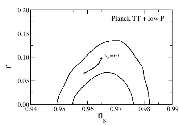
Figure 1: Predictions for $n_{s}$ and $r$ (shown in Table 1) as obtained from the deformed version of standard chaotic inflation are indicated by dark dots with $N_{e}=60$. A solid line joining them represents the predictions for $n_{s}$ and $r$ while $\alpha$ is varied. $1\sigma$ and $2\sigma$ contours of $n_{s}-r$ as obtained from Planck 2015 data[12] are included for reference.

Planck 2015 [12]. We take $N_{e}$ as 60. Few of our findings for $n_{s}$ and $r$ in terms of the parameters $m$ and $\alpha$ are provided in the Table 1. In Fig.1 we show our predictions for $n_{s}$ and $r$ by four dark dots joined by a line. The dark dots represent the four sets of parameters mentioned in Table 1. Along the line joining these, the parameter $\alpha$ is varied and correspondingly the magnitude of $\tilde{m}$ is adjusted mildly (as seen from Table 1) in order to keep the curvature perturbation unchanged. The 1$\sigma$ and 2$\sigma$ contours from the Planck 2015[12] are also depicted as reference in Fig.1. As an example with $\alpha\sim 7\times 10^{-4}$ and $N_{e}=60$, we find $\tilde{\phi^{*}}\simeq 14.85$ (inflaton field value at horizon exit) and $\tilde{\phi}_{end}\simeq\sqrt{2}$ (field value at the end of inflation). Hence the slow roll parameters $\epsilon$ and $\eta$ can be obtained at $\tilde{\phi}=\tilde{\phi}^{*}$ and we can determine $n_{s}$ and $r$. The parameter $m$ is fixed by the required value of curvature perturbation $P_{s}=2.2\times 10^{-9}$[12]. $\tilde{m}$ is found to be $5.83\times 10^{-6}$ for the above values of $\alpha$ and $N_{e}$. As expected we obtain a smaller value of $r\sim 0.097$ compared to the standard chaotic inflation with $r\sim 0.133$ (and $n_{s}\simeq 0.966$) as seen from Table 1 (first set).

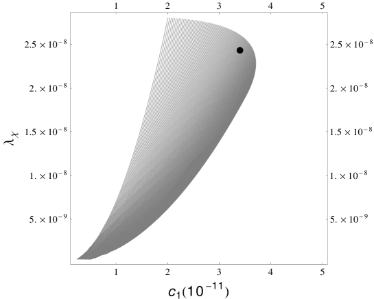
Figure 2: Allowed region of $c_{1}$ (in unit of $10^{-11}$) and $\lambda_{\chi}$ is indicated by the shadowed region where the constraints [(i)-(v)] are included. The black dot represents the reference value of $c_{1}\simeq\tilde{m}^{2}=3.39\times 10^{-11}$ and $\lambda_{\chi}\simeq 2.43\times 10^{-8}$. $\alpha$ satisfies $2.7\times 10^{-4}<\alpha<2.5\times 10^{-3}$.

Let us now proceed to determine the allowed range of parameters $c_{1}$ and $\lambda_{\chi}$ from estimate of $\alpha$ and $m$ we found above. For this purpose, we first summarize the relevant points already discussed. Specifically, during inflation:(i) $m_{\chi}^{2}>H_{\textrm{Inf}}^{2}$ ,which indicates $c_{1}/\tilde{m}^{2}>1/12$ or equivalently $\lambda_{\chi}>\frac{\tilde{m}^{2}}{288\alpha}$. (ii) We assume $\chi$ field as sub-Planckian at the onset of inflation and afterwards. Hence $\tilde{\chi}_{\textrm{I}}\simeq(c_{1}/\lambda_{\chi})\tilde{\phi}<1$. (iii) As explained below in Eq.(6) we consider $\alpha\tilde{\phi}^{2}<1$.(iv) However note that this term should be sufficiently large so as to produce significant (at least ten percent) change in $r$ as compared to the minimal chaotic inflation. Ten percent or more reduction of $r$ can be achieved with $\alpha\tilde{\phi}^{2}\geq 0.05$. Therefore $\alpha$ is bounded by the inequality $0.05\leq\alpha\tilde{\phi}^{2}<1$. Note that one can find $\tilde{\phi}^{*}(\alpha)$ (as function of $\alpha$) by solving $N_{e}=60$ for a specific choice of $\alpha$. Using the fact that we only keep terms of the order $\alpha\tilde{\phi}^{2}$ (i.e neglecting higher order terms), a suitable upper value of $\alpha\tilde{\phi}^{2}$ can be chosen as $\alpha\tilde{\phi}^{2}<0.4$. Then plugging $\tilde{\phi}^{*}$ as a function of $\alpha$, we obtain $2.7\times 10^{-4}\leq\alpha\leq 2.5\times 10^{-3}$ as shown in Fig. 2. To be concrete for the sake of discussion we choose a particular value of $\alpha$ within this range, say $\alpha=7\times 10^{-4}$ (see the first set of Table 1). One such $\alpha$ corresponds to a particular $\tilde{m}$ value through Eq.(9) to have $P_{s}=2.2\times 10^{-9}$ while $\tilde{\phi}^{*}$ is replaced by $\alpha-$dependence. Hence condition (i) can be translated as $\lambda_{\chi}>1.68\times 10^{-10}$ for $\alpha=7\times 10^{-4}$. (v) An upper bound of $\lambda_{\chi}$ can be set from the requirement that involves the initial condition problem. Note that the universe during the inflation is expected to be dominated by the $\phi$ field and hence $\lambda_{\chi}\chi^{4}/4$ term should be sub-dominated compared to $(1/2)m^{2}\phi^{2}$ while initial $\tilde{\phi}^{*}$ can be large enough during the Planckian time and $\tilde{\chi}^{*}$ (initial value of $\chi$ before inflation starts) should remain sub-Planckian. For example considering $\tilde{\phi}^{*}\simeq 16$ and $\tilde{\chi}^{*}\simeq 0.9$, we have $\lambda_{\chi}<2.7\times 10^{-8}$ such that $\lambda_{\chi}\tilde{\chi}^{4}/4<(1/2)\tilde{m}^{2}\tilde{\phi}^{2}$. So $\lambda_{\chi}$ is restricted by $1.67\times 10^{-10}<\lambda_{\chi}<2.7\times 10^{-8}$. From this we note that a choice $c_{1}=\tilde{m}^{2}$ falls in the right ballpark which corresponds to $\lambda_{\chi}=(c_{1}/2\alpha)=2.43\times 10^{-8}$. Considering the range of $\alpha$ as obtained, the allowed parameter space for $c_{1}$ and $\lambda_{\chi}$ are shown in Fig.2 where the point corresponding to $c_{1}=\tilde{m}^{2}$ and $\lambda_{\chi}=2.43\times 10^{-8}$ is denoted by a dark dot.

We now turn our attention to the other part of the work which involves the SM Higgs doublet $H$ and its interaction with the inflation sector. The relevant tree level potential is given by

$$V_{\textrm{II}}=\lambda_{H}\Big{(}H^{\dagger}H-\frac{v^{2}}{2}\Big{)}^{2}+\frac{\lambda_{\chi H}}{2}(\chi^{2}-v_{\chi}^{2})\Big{(}H^{\dagger}H-\frac{v^{2}}{2}\Big{)}+\frac{\lambda_{\phi H}}{2}\phi^{2}\Big{(}H^{\dagger}H-\frac{v^{2}}{2}\Big{)}.$$ (10)

As discussed earlier we expect the threshold effect on the running of the Higgs quartic coupling to appear from its interaction with the $\chi$ field only as $\langle\chi\rangle$ can be large while $\langle\phi\rangle=0$. Hence we drop the last term involving interaction between $H$ and inflaton $\phi$ for the rest of our discussion by assuming $\lambda_{\phi H}$ vanishingly small. To explore the stability of the Higgs potential we need to consider the $\lambda_{\chi}$ term from Eq.(2) as well. The part of the entire potential $V_{\textrm{I}}+V_{\textrm{II}}$ relevant to discuss the vacuum stability issue is therefore given by

$$V_{0}=\lambda_{H}\Big{(}H^{\dagger}H-\frac{v^{2}}{2}\Big{)}^{2}+\frac{\lambda_{\chi H}}{2}(\chi^{2}-v_{\chi}^{2})\Big{(}H^{\dagger}H-\frac{v^{2}}{2}\Big{)}+\frac{\lambda_{\chi}}{4}(\chi^{2}-v_{\chi}^{2})^{2}.$$ (11)

The minimum of $V_{0}$ is given by

$$\langle H^{\dagger}H\rangle=\frac{v^{2}}{2}\textrm{, }\langle\chi\rangle=v_{\chi},$$ (12)

where we have considered $\lambda_{H}$, $\lambda_{\chi}>0$. Note that the above minimum of $V_{0}$ (the EW minimum) corresponds to vanishing vacuum energy i.e. $V_{0}^{\textrm{EW}}=0$. Now in order to maintain the stability of the potential, $V_{0}$ should remain positive ($V_{0}>0$) even when the fields involved ($\chi$ and $H$) are away from their respective values at the EW minimum. Since the couplings depend on the renormalization scale $\mu$ $(\sim$ field value) we must ensure $\lambda_{\chi}(\mu)$, $\lambda_{H}(\mu)>0$ in order to avoid any deeper minimum (lower than the $V_{0}^{\textrm{EW}}$) away from the EW one.

In order to study the running of all the couplings under consideration, we consider the renormalization group (RG) equations for them. Below we provide the RG equations for $\lambda_{H}$, $\lambda_{\chi H}$ and $\lambda_{\chi}$[24] as

$$\frac{d\lambda_{H}}{dt}= \beta^{SM}_{\lambda_{H}}+\frac{1}{16\pi^{2}}\lambda_{\chi H}^{2},$$ (13)

$$\frac{d\lambda_{\chi H}}{dt}= \frac{1}{16\pi^{2}}\Big{\{}12\lambda_{H}\lambda_{\chi H}+8\lambda_{\chi}\lambda_{\chi H}+4\lambda_{\chi H}^{2}+6y_{t}^{2}\lambda_{\chi H}-\frac{3}{2}g_{1}^{2}\lambda_{\chi H}-\frac{9}{2}g_{2}^{2}\lambda_{\chi H}\Big{\}},$$ (14)

$$\frac{d\lambda_{\chi}}{dt}= \frac{1}{16\pi^{2}}\Big{\{}20\lambda_{\chi}^{2}+2\lambda_{\chi H}^{2}\Big{\}}.$$ (15)

$\beta^{SM}_{\lambda_{H}}$is the three loop $\beta$-function for the Higgs quartic coupling[24] in SM, which is corrected by the one-loop contribution in presence of the $\chi$ field. The RG equation for two new physics parameters $\lambda_{\chi H}$ and $\lambda_{\chi}$ are kept at one loop. The presence of the $\chi$ field is therefore expected to modify the stability conditions above its mass $m_{\chi}$.

Apart from the modified running of the Higgs quartic coupling, vacuum stability is also affected by the presence of the threshold correction from the heavy $\chi$ field which carries a large vev. The mass of the $\chi$ field is given by $m_{\chi}=\sqrt{2\lambda_{\chi}}v_{\chi}$ (see Eq.(4) with $\phi=0$ after inflation), the heavy field $\chi$ can be integrated out below $m_{\chi}$. By solving the equation of motion of $\chi$ field we have

$$\chi^{2}\simeq v_{\chi}^{2}-\frac{\lambda_{\chi H}}{\lambda_{\chi}}\Big{(}H^{\dagger}H-\frac{v^{2}}{2}\Big{)}.$$ (16)

Hence below the scale $m_{\chi}$, the effective potential of $V_{0}$ becomes

$$V_{0}^{\textrm{eff}}\simeq\lambda_{h}\Big{(}H^{\dagger}H-\frac{v^{2}}{2}\Big{)}^{2},\textrm{ with }\lambda_{h}({m_{\chi}})=\Big{[}\lambda_{H}-\frac{\lambda_{\chi H}^{2}}{4\lambda_{\chi}}\Big{]}_{m_{\chi}},$$ (17)

where Eq.(16) is used to replace $\chi$ into Eq.(11). Therefore below $m_{\chi}$, $\lambda_{h}$ corresponds to the SM Higgs quartic coupling and above $m_{\chi}$ it gets a positive shift $\delta\lambda=\frac{\lambda_{\chi H}^{2}}{4\lambda_{\chi}}$. This could obviously help in delaying the Higgs quartic coupling to become negative provided $m_{\chi}$ is below the SM instability scale, i.e. $m_{\chi}<\Lambda_{I}^{\textrm{SM}}$. In this analysis, we investigate the parameter space for which the Higgs quartic coupling remains positive upto the scale $M_{P}$. This however depends upon $m_{\chi}$ and $\delta\lambda$. Note that $\lambda_{\chi}$ involved in both $m_{\chi}$ and $\delta\lambda$ which is somewhat restricted from inflation (see Fig.2). On the other hand $v_{\chi}$ is not restricted from inflation. We will have an estimate of $v_{\chi}$ by requiring $m_{\chi}<\Lambda_{I}^{\textrm{SM}}$ (using a specific $\lambda_{\chi}$ value corresponding to set-1 of Table 1.) We also consider $\delta\lambda\sim\lambda_{h}({m_{\chi}})$ to avoid un-naturalnes in the amount of shift. This consideration in turn fixes $\lambda_{\chi H}$.

Once the electroweak symmetry is broken, the diagonalization of the mass-square matrix involving quadratic terms of $\chi$, $H$ and their mixing ($\lambda_{\chi H}$ term) yields one light and one heavy scalars. Using the unitary gauge for redefining the Higgs doublet as $H^{T}=\Big{(}0,\frac{v+h}{\sqrt{2}}\Big{)}$, the masses associated with the light and heavy eigenstates are

$$m^{2}_{\textrm{$h$,$h_{H}$}}=\Big{[}\lambda_{H}v^{2}+\lambda_{\chi}v_{\chi}^{2}\mp\sqrt{\Big{(}\lambda_{H}v^{2}-\lambda_{\chi}v_{\chi}^{2}\Big{)}^{2}+\lambda_{\chi H}^{2}v^{2}v_{\chi}^{2}}\Big{]},$$ (18)

where $h$ and $h_{H}$ correspond to light and heavy Higgs. In the limit of small mixing angle $\theta=\Big{[}\frac{1}{2}\textrm{tan}^{-1}\frac{\lambda_{\chi H}v_{\chi}v}{\lambda_{H}v^{2}-\lambda_{\chi}v_{\chi}^{2}}$], $m_{h}$ becomes $m_{h}\simeq\sqrt{2}v\Big{(}\lambda_{H}-\frac{\lambda_{\chi H}^{2}}{4\lambda_{\chi}}\Big{)}$ with $\lambda_{\chi}v_{\chi}^{2}\gg\lambda_{H}v^{2}$. In order to avoid the unwanted negative value of $m_{h}$, the extra stability condition $4\lambda_{\chi}\lambda_{H}>\lambda_{\chi H}^{2}$ should be maintained (with $\lambda_{\chi H}>0$). However it is pointed out in [24] that it is sufficient that this condition should be satisfied for a short interval around $m_{\chi}$ for $\lambda_{\chi H}>0$. However for $\lambda_{\chi H}<0$, this extra stability condition becomes $2\sqrt{\lambda_{\chi}(\mu)\lambda_{H}(\mu)}+\lambda_{\chi H}(\mu)>0$. As found in [24], it is difficult to achieve the absolute stability of $V_{0}$ till $M_{P}$ in this case. We restrict ourselves into the case $\lambda_{\chi H}>0$ for the present work.

Scale ($\mu$)	$y_{t}$	$g_{1}$	$g_{2}$	$g_{3}$	$\lambda_{h}$
$m_{t}$	$0.93668$	$0.357632$	$0.648228$	$1.166508$	$0.127102$

Table 2: Values of couplings in SM at $m_{t}=173.3$ GeV.

To have a concrete understanding of the vacuum stability issue in this set-up, we first estimate several parameters at a scale of top quark mass $m_{t}=$173.3 GeV. The values of the top quark Yukawa coupling ($y_{t}$), gauge couplings ($g_{i}$) and Higgs quartic coupling $\lambda_{h}$ are taken at two loop NNLO precision following [10]. These are mentioned in Table 2. We then use the RG equations (Eqns.(13-15)) for these parameters to study the running of $\lambda_{h}$ as shown in Fig. 3. We also consider the three loop SM RGE for the gauge couplings. The instability scale then turns out to be $\Lambda_{I}^{\textrm{SM}}\simeq 1.2\times 10^{10}$ GeV for $m_{t}=173.3$ GeV, $m_{h}=125.66$ GeV and $\alpha_{s}(M_{Z})=0.1184$.

Scale($\mu$)	$\lambda_{\chi}$	$\lambda_{\chi H}$	$y_{t}$	$g_{1}$	$g_{2}$	$g_{3}$	$\lambda_{H}$
$m_{\chi}$	$2.38\times 10^{-8}$	$3.66\times 10^{-5}$	$0.59523$	$0.386864$	$0.58822$	$0.72327$	$0.0278$
$M_{P}$	$2.45\times 10^{-8}$	$3.56\times 10^{-5}$	$0.39112$	$0.467056$	$0.509155$	$0.49591$	$\mathcal{O}(10^{-5})$

Table 3: Values of couplings at $m_{\chi}$ and $M_{P}$ for $m_{\chi}=8\times 10^{7}$ GeV and $m_{t}=173.3$ GeV.

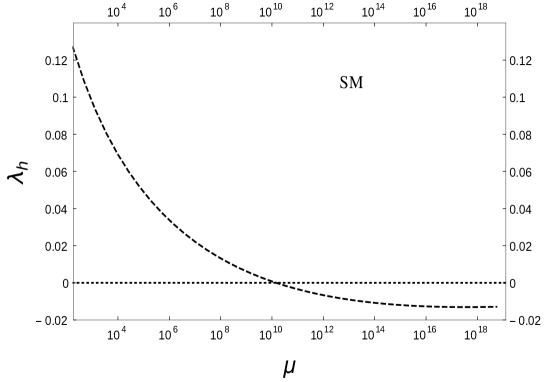
Figure 3: Running of the SM Higgs quartic coupling till $M_{P}$ is shown for $m_{t}=173.3$ GeV, $m_{h}=125.66$ GeV and $\alpha_{s}(M_{Z})=0.1184$.

Let us now proceed to the case with SM+Inflation extension. In this case, above the energy scale $m_{\chi}$, two other couplings $\lambda_{\chi}$ and $\lambda_{\chi H}$ will appear as in Eq.(11). As discussed earlier, we already have an estimate of $\lambda_{\chi}$ to have successful results in inflation sector with $c_{1}=\tilde{m}^{2}$.

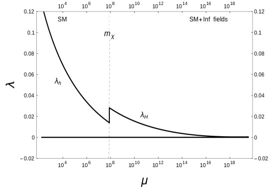
Figure 4: Running of Higgs quartic coupling till $M_{P}$ for $\lambda_{\chi H}({m_{\chi}})=3.66\times 10^{-5},\lambda_{\chi}({m_{\chi}})=2.38\times 10^{-8}$ with $m_{\chi}=8\times 10^{7}$ GeV.

We consider the corresponding value of $\lambda_{\chi}=2.43\times 10^{-8}$ at inflation scale $\Lambda_{\textrm{Inf}}\sim V_{\textrm{Inf}}^{1/4}\simeq 10^{16}$ GeV. The initial value of $\lambda_{\chi}$ should be fixed at $m_{\chi}$ (remains same at $m_{t}$) in such a way that it can reproduce $\lambda_{\chi}$($\Lambda_{\textrm{Inf}}$) correctly through its RG equation in Eq.(15). $\lambda_{\chi H}$ $(m_{\chi})$ is chosen to achieve a natural enhancement $\delta\lambda\sim\lambda_{h}(m_{\chi})$ at $m_{\chi}$. Hereafter above $m_{\chi}$, the Higgs quartic coupling $\lambda_{H}$ is governed through the modified RG equation as in Eq.(13). Note that even if $\lambda_{\chi}$ is known it does not fix $m_{\chi}$($=\sqrt{2\lambda_{\chi}}v_{\chi}$) completely. Therefore we can vary $v_{\chi}$ to have $m_{\chi}<\Lambda_{I}^{\textrm{SM}}$.

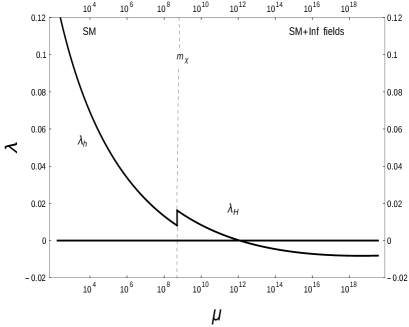
(a)

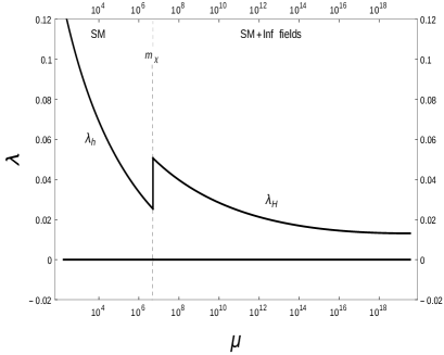
(b)

Figure 5: Running of Higgs quartic coupling till $M_{P}$ for (a) $m_{\chi}(=5\times 10^{8}\textrm{ GeV})>m_{C}$, (b) $m_{\chi}(=5\times 10^{6}\textrm{ GeV})<m_{C}$. We consider $\delta\lambda=\lambda_{h}(m_{\chi})$ which corresponds to the choice for (a) $\lambda_{\chi H}({m_{\chi}})=2.8\times 10^{-5}$, $\lambda_{\chi}({m_{\chi}})=2.4\times 10^{-8}$ and (b) $\lambda_{\chi H}({m_{\chi}})=4.88\times 10^{-5},\lambda_{\chi}({m_{\chi}})=2.35\times 10^{-8}$ respectively.

With the above mentioned scheme, we study the running of the Higgs quartic coupling for different $m_{\chi}$ satisfying $m_{\chi}<\Lambda_{I}^{\textrm{SM}}$. We find that with $m_{\chi}=8\times 10^{7}$ GeV, $\lambda_{H}$ becomes vanishingly small at $M_{P}$ (hence the new instability scale $\Lambda_{I}$ becomes $\sim M_{P}$) as shown in Fig.4. We specify the corresponding $m_{\chi}$ value as $m_{C}(=8\times 10^{7}$ GeV). The other relevant couplings at $m_{\chi}$ and at $M_{P}$ are given in Table 3. It is then observed that in order to keep the Higgs quartic coupling positive all the way upto $M_{P}$, we should ensure $m_{\chi}<m_{C}$. For example with $m_{\chi}=5\times 10^{8}$ GeV ($>m_{c}$) we see $\lambda_{H}$ becomes negative at scale $\sim 10^{12}$ GeV as shown in Fig.5(a). On the other hand in Fig.5(b) it is seen that $\lambda_{H}$ remains positive till $M_{P}$ for $m_{\chi}\sim 5\times 10^{6}$ GeV $<m_{C}$. In doing so we consider the amount of positive shift at $m_{\chi}$ to be defined with $\delta\lambda\sim\lambda_{h}(m_{\chi})$. In Fig.6 we provide the variation of instability scale $\Lambda_{I}$ (which is atmost $\sim M_{P}$ for $m_{\chi}=m_{C}$ case) in SM+Inflation extension if we relax this assumption by changing $\delta\lambda$ arbitarily. To give a feeling about how other couplings are changing with $\mu$, we plot running of gauge couplings $g_{i=1,2,3}$, top quark yukawa coupling $y_{t}$, $\lambda_{\chi}$, $\lambda_{H}$ and $\lambda_{\chi H}$ in Fig.7 with $m_{\chi}=m_{C}=8\times 10^{7}$ GeV.

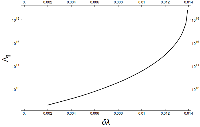
Figure 6: Variation of instability scale $\Lambda_{I}$ with change of $\delta\lambda$ where $m_{\chi}=m_{C}\simeq 8\times 10^{7}$ GeV.

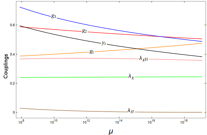
Figure 7: Running of the couplings $g_{i=1,2,3}$, $y_{t}$, $\lambda_{H}$, $\lambda_{\chi H}$ (in unit of $10^{-4}$) and $\lambda_{\chi}$ (in unit of $10^{-7}$) in SM+Inflation scenario from $m_{\chi}=m_{C}\sim 8\times 10^{7}$ GeV to $M_{P}$.

For completeness we now comment on reheating in the present set-up. Once the inflation ends, the inflaton $\phi$ will oscillate around the minimum at $\phi=0$. The decay of $\phi$ would then proceed provided it interacts with the SM fields. Here we do not attempt to discuss it in details. Instead we only mention about the possibilities. The details will be discussed elsewhere in a future study. We may consider terms in the Lagrangian as

$$-\mathcal{L}_{int}=y_{\phi}\phi NN+y_{\nu}\bar{L}\tilde{H}N,$$ (19)

where $N$ is the right handed (RH) neutrino and $L$ is the SM lepton doublet. $y_{\phi}$, $y_{\nu}$ are the respective couplings. Note that the first term is an explicit $Z_{2}$ breaking term and hence $y_{\phi}$ is expected to be small in the present set-up. The corresponding reheat temperature is then found to be $T_{r}\simeq y_{\phi}\sqrt{\frac{mM_{P}}{8\pi}}\sim 10^{15}y_{\phi}$ GeV where we have used $m=1.4\times 10^{13}$ GeV from set-1, Table 1. A further decay of RH neutrinos into $L$ and $H$ can be responsible for leptogenesis [51, 52, 53, 54, 55]. The term $y_{\phi}\phi NN$ can not however provide the mass of the RH neutrinos as $\langle\phi\rangle=0$. A mass term like $M_{N}NN$ has to be present. If we turn our attention to the other field $\chi$ involved in the inflation sector, we note that this field will oscillate about $\langle\chi\rangle$ at the end of inflation. The decays of it can proceed via $\chi\rightarrow hh$ with $\Gamma_{\chi}=\frac{\lambda_{\chi H}^{2}m_{\chi}}{256\pi\lambda_{\chi}}$. Then two cases may arise; (i) $\Gamma_{\phi}\ll\Gamma_{\chi}$: in this case the $\chi$ field will decay very fast. However reheat of universe will finish much later after $\chi$ field decay. So any radiation energy density produced by $\chi$ will be strongly diluted during the matter dominated phase governed by the oscillations of $\phi$. (ii) $\Gamma_{\phi}\gg\Gamma_{\chi}$: note that energy density of the $\chi$ field is much less than that of $\phi$ and universe will reheat once decay of $\phi$ field is completed. Hence the completion of the inflaton decay into radiation, when Hubble becomes of order $\Gamma_{\chi}$, $\chi$ field will decay to radiation. So the remnant radiation in this case will be a mixture of $\phi$ and $\chi$ products.

The discovery of the Higgs boson and the precise determination of its mass at LHC provide us an estimate of the Higgs quartic coupling in the SM. However the high scale behavior of this coupling, whether or not it becomes negative, poses plethora of questions in terms of the stabilization of the electroweak minimum. Though the present data favors the metastability of this vacuum, it is very much dependent on the precision of the top mass measurement. Furthermore inflation in the early universe provides additional threat as it can shift the Higgs field during inflation into the unwanted part of the Higgs potential and hence metastability can also be questioned. As a resolution to this, we propose introduction of the inflation sector consisting of two scalar fields $\phi$ and $\chi$ and their interaction with the SM Higgs. While $\phi$ is playing the role of the inflaton having the potential $m^{2}\phi^{2}/2$, the other field $\chi$ provides a deviation in terms of prediction of the spectral index and tensor to scalar ratio so has to be consistent with the Planck 2015 data. We have shown that the $\chi$-Higgs coupling can have profound effect in the running of Higgs quartic coupling considering the positive shift through the threshold effect at a scale $m_{\chi}$. It turns out the quartic coupling of the $\chi$ field is restricted to achieve successful inflation. This in turn constrain the other new physics parameters space if we want to make the Higgs potential completely stable upto $M_{P}$. The scenario also alleviates the problem of instability of the EW vacuum during inflation as the Higgs field is stabilized at origin having a mass larger($\sim 100H_{\textrm{Inf}}^{2}$) than the Hubble during inflation. Once the inflation is over, it smoothly enters into the near EW minimum. We have also commented on the possible reheating scenario in brief. The vev of the $\chi$ field breaks the $Z_{2}$ symmetry which may spontaneously lead to domain wall problem. An explicit $Z_{2}$- symmetry breaking term or gauging the symmetry would help in resolving the issue. As an extension of our present set-up, one can possibly consider a $U(1)_{B-L}$ embedding of the entire framework where the neutrino masses and several other related aspects like effect of gauge bosons on running etc. can be simultaneously addressed.

References

- [1] K. A. Olive et al. [Particle Data Group Collaboration], Chin. Phys. C 38, 090001 (2014). doi:10.1088/1674-1137/38/9/090001
- [2] G. Aad et al. [ATLAS Collaboration], Phys. Lett. B 716, 1 (2012) doi:10.1016/j.physletb.2012.08.020 [arXiv:1207.7214 [hep-ex]].
- [3] S. Chatrchyan et al. [CMS Collaboration], Phys. Lett. B 716, 30 (2012) doi:10.1016/j.physletb.2012.08.021 [arXiv:1207.7235 [hep-ex]].
- [4] P. P. Giardino, K. Kannike, I. Masina, M. Raidal and A. Strumia, JHEP 1405, 046 (2014) doi:10.1007/JHEP05(2014)046 [arXiv:1303.3570 [hep-ph]].
- [5] S. R. Coleman and E. J. Weinberg, Phys. Rev. D 7, 1888 (1973). doi:10.1103/PhysRevD.7.1888
- [6] M. Sher, Phys. Rept. 179, 273 (1989). doi:10.1016/0370-1573(89)90061-6
- [7] V. Branchina, E. Messina and A. Platania, JHEP 1409, 182 (2014) doi:10.1007/JHEP09(2014)182 [arXiv:1407.4112 [hep-ph]].
- [8] G. Degrassi, Nuovo Cim. C 037, no. 02, 47 (2014) doi:10.1393/ncc/i2014-11735-1 [arXiv:1405.6852 [hep-ph]].
- [9] G. Isidori, G. Ridolfi and A. Strumia, Nucl. Phys. B 609, 387 (2001) doi:10.1016/S0550-3213(01)00302-9 [hep-ph/0104016].
- [10] D. Buttazzo, G. Degrassi, P. P. Giardino, G. F. Giudice, F. Sala, A. Salvio and A. Strumia, JHEP 1312, 089 (2013) doi:10.1007/JHEP12(2013)089 [arXiv:1307.3536 [hep-ph]].
- [11] Y. Tang, Mod. Phys. Lett. A 28, 1330002 (2013) doi:10.1142/S0217732313300024 [arXiv:1301.5812 [hep-ph]].
- [12] P. A. R. Ade et al. [Planck Collaboration], arXiv:1502.01589 [astro-ph.CO].
- [13] A. Kobakhidze and A. Spencer-Smith, Phys. Lett. B 722, 130 (2013) doi:10.1016/j.physletb.2013.04.013 [arXiv:1301.2846 [hep-ph]].
- [14] C. Gross, O. Lebedev and M. Zatta, Phys. Lett. B 753, 178 (2016) doi:10.1016/j.physletb.2015.12.014 [arXiv:1506.05106 [hep-ph]].
- [15] A. D. Linde, Lect. Notes Phys. 738, 1 (2008) doi:10.1007/978-3-540-74353-81 [arXiv:0705.0164 [hep-th]].
- [16] K. Harigaya, M. Ibe, M. Kawasaki and T. T. Yanagida, Phys. Lett. B 756, 113 (2016) doi:10.1016/j.physletb.2016.03.001 [arXiv:1506.05250 [hep-ph]].
- [17] J. L. Evans, T. Gherghetta and M. Peloso, Phys. Rev. D 92, no. 2, 021303 (2015) doi:10.1103/PhysRevD.92.021303 [arXiv:1501.06560 [hep-ph]].
- [18] A. K. Saha and A. Sil, JHEP 1511, 118 (2015) doi:10.1007/JHEP11(2015)118 [arXiv:1509.00218 [hep-ph]].
- [19] R. Kallosh and A. Linde, JCAP 1011, 011 (2010) doi:10.1088/1475-7516/2010/11/011 [arXiv:1008.3375 [hep-th]].
- [20] T. Li, Z. Li and D. V. Nanopoulos, JCAP 1402, 028 (2014) doi:10.1088/1475-7516/2014/02/028 [arXiv:1311.6770 [hep-ph]].
- [21] K. Harigaya, M. Ibe, K. Schmitz and T. T. Yanagida, Phys. Lett. B 720, 125 (2013) doi:10.1016/j.physletb.2013.01.058 [arXiv:1211.6241 [hep-ph]].
- [22] K. Nakayama, F. Takahashi and T. T. Yanagida, Phys. Lett. B 725, 111 (2013) doi:10.1016/j.physletb.2013.06.050 [arXiv:1303.7315 [hep-ph]].
- [23] K. Harigaya, M. Kawasaki and T. T. Yanagida, Phys. Lett. B 741, 267 (2015) doi:10.1016/j.physletb.2014.12.053 [arXiv:1410.7163 [hep-ph]].
- [24] J. Elias-Miro, J. R. Espinosa, G. F. Giudice, H. M. Lee and A. Strumia, JHEP 1206, 031 (2012) doi:10.1007/JHEP06(2012)031 [arXiv:1203.0237 [hep-ph]].
- [25] L. A. Anchordoqui, I. Antoniadis, H. Goldberg, X. Huang, D. Lust, T. R. Taylor and B. Vlcek, JHEP 1302, 074 (2013) doi:10.1007/JHEP02(2013)074 [arXiv:1208.2821 [hep-ph]].
- [26] K. Bhattacharya, J. Chakrabortty, S. Das and T. Mondal, JCAP 1412, no. 12, 001 (2014) doi:10.1088/1475-7516/2014/12/001 [arXiv:1408.3966 [hep-ph]].
- [27] Y. Ema, K. Mukaida and K. Nakayama, arXiv:1605.07342 [hep-ph].
- [28] S. Baek, P. Ko, W. I. Park and E. Senaha, JHEP 1211, 116 (2012) doi:10.1007/JHEP11(2012)116 [arXiv:1209.4163 [hep-ph]].
- [29] M. Gonderinger, Y. Li, H. Patel and M. J. Ramsey-Musolf, JHEP 1001, 053 (2010) doi:10.1007/JHEP01(2010)053 [arXiv:0910.3167 [hep-ph]].
- [30] M. Gonderinger, H. Lim and M. J. Ramsey-Musolf, Phys. Rev. D 86, 043511 (2012) doi:10.1103/PhysRevD.86.043511 [arXiv:1202.1316 [hep-ph]].
- [31] W. Chao, M. Gonderinger and M. J. Ramsey-Musolf, Phys. Rev. D 86, 113017 (2012) doi:10.1103/PhysRevD.86.113017 [arXiv:1210.0491 [hep-ph]].
- [32] C. S. Chen and Y. Tang, JHEP 1204, 019 (2012) doi:10.1007/JHEP04(2012)019 [arXiv:1202.5717 [hep-ph]].
- [33] N. Khan and S. Rakshit, Phys. Rev. D 90, no. 11, 113008 (2014) doi:10.1103/PhysRevD.90.113008 [arXiv:1407.6015 [hep-ph]].
- [34] V. V. Khoze, C. McCabe and G. Ro, JHEP 1408, 026 (2014) doi:10.1007/JHEP08(2014)026 [arXiv:1403.4953 [hep-ph]].
- [35] Y. Mambrini, N. Nagata, K. A. Olive and J. Zheng, arXiv:1602.05583 [hep-ph].
- [36] S. Khan, S. Goswami and S. Roy, Phys. Rev. D 89, no. 7, 073021 (2014) doi:10.1103/PhysRevD.89.073021 [arXiv:1212.3694 [hep-ph]].
- [37] A. Datta, A. Elsayed, S. Khalil and A. Moursy, Phys. Rev. D 88, no. 5, 053011 (2013) doi:10.1103/PhysRevD.88.053011 [arXiv:1308.0816 [hep-ph]].
- [38] J. Chakrabortty, P. Konar and T. Mondal, Phys. Rev. D 89, no. 5, 056014 (2014) doi:10.1103/PhysRevD.89.056014 [arXiv:1308.1291 [hep-ph]].
- [39] A. Kobakhidze and A. Spencer-Smith, JHEP 1308, 036 (2013) doi:10.1007/JHEP08(2013)036 [arXiv:1305.7283 [hep-ph]].
- [40] S. Baek, H. Okada and T. Toma, JCAP 1406, 027 (2014) doi:10.1088/1475-7516/2014/06/027 [arXiv:1312.3761 [hep-ph]].
- [41] C. Coriano, L. Delle Rose and C. Marzo, Phys. Lett. B 738, 13 (2014) doi:10.1016/j.physletb.2014.09.001 [arXiv:1407.8539 [hep-ph]].
- [42] R. N. Mohapatra and Y. Zhang, JHEP 1406, 072 (2014) doi:10.1007/JHEP06(2014)072 [arXiv:1401.6701 [hep-ph]].
- [43] N. Haba and Y. Yamaguchi, PTEP 2015, no. 9, 093B05 (2015) doi:10.1093/ptep/ptv121 [arXiv:1504.05669 [hep-ph]].
- [44] L. Delle Rose, C. Marzo and A. Urbano, JHEP 1512, 050 (2015) doi:10.1007/JHEP12(2015)050 [arXiv:1506.03360 [hep-ph]].
- [45] A. Das, N. Okada and N. Papapietro, arXiv:1509.01466 [hep-ph].
- [46] C. Bonilla, R. M. Fonseca and J. W. F. Valle, Phys. Lett. B 756, 345 (2016) doi:10.1016/j.physletb.2016.03.037 [arXiv:1506.04031 [hep-ph]].
- [47] N. Haba, H. Ishida, N. Okada and Y. Yamaguchi, Eur. Phys. J. C 76, no. 6, 333 (2016) doi:10.1140/epjc/s10052-016-4180-z [arXiv:1601.05217 [hep-ph]].
- [48] J. N. Ng and A. de la Puente, Eur. Phys. J. C 76, no. 3, 122 (2016) doi:10.1140/epjc/s10052-016-3981-4 [arXiv:1510.00742 [hep-ph]].
- [49] K. Mukaida and K. Nakayama, JCAP 1408, 062 (2014) doi:10.1088/1475-7516/2014/08/062 [arXiv:1404.1880 [hep-ph]].
- [50] A. Salvio and A. Mazumdar, Phys. Lett. B 755, 469 (2016) doi:10.1016/j.physletb.2016.02.057 [arXiv:1512.08184 [hep-ph]].
- [51] M. Fukugita and T. Yanagida, Phys. Lett. B 174, 45 (1986). doi:10.1016/0370-2693(86)91126-3
- [52] M. Flanz, E. A. Paschos and U. Sarkar, Phys. Lett. B 345, 248 (1995) Erratum: [Phys. Lett. B 384, 487 (1996)] Erratum: [Phys. Lett. B 382, 447 (1996)] doi:10.1016/0370-2693(96)00866-0, 10.1016/0370-2693(96)00842-8, 10.1016/0370-2693(94)01555-Q [hep-ph/9411366].
- [53] L. Covi, E. Roulet and F. Vissani, Phys. Lett. B 384, 169 (1996) doi:10.1016/0370-2693(96)00817-9 [hep-ph/9605319].
- [54] M. Plumacher, Z. Phys. C 74, 549 (1997) doi:10.1007/s002880050418 [hep-ph/9604229].
- [55] W. Buchmuller and M. Plumacher, Phys. Lett. B 431, 354 (1998) doi:10.1016/S0370-2693(97)01548-7 [hep-ph/9710460].
- [56] W. Buchmuller, P. Di Bari and M. Plumacher, Annals Phys. 315, 305 (2005) doi:10.1016/j.aop.2004.02.003 [hep-ph/0401240].