Entanglement entropy of the Qโ‰ฅ4๐‘„4Q\geq 4 quantum Potts chain

Pรฉter Lajkรณ peter.lajko@ku.edu.kw Department of Physics, Kuwait University, P.O. Box 5969, Safat 13060, Kuwait โ€ƒโ€ƒ Ferenc Iglรณi igloi.ferenc@wigner.mta.hu Wigner Research Centre, Institute for Solid State Physics and Optics, H-1525 Budapest, P.O.Box 49, Hungary Institute of Theoretical Physics, Szeged University, H-6720 Szeged, Hungary
Abstract

The entanglement entropy, ๐’ฎ๐’ฎ{\cal S}, is an indicator of quantum correlations in the ground state of a many body quantum system. At a second-order quantum phase-transition point in one dimension ๐’ฎ๐’ฎ{\cal S} generally has a logarithmic singularity. Here we consider quantum spin chains with a first-order quantum phase transition, the prototype being the Q๐‘„Q-state quantum Potts chain for Q>4๐‘„4Q>4 and calculate ๐’ฎ๐’ฎ{\cal S} across the transition point. According to numerical, density matrix renormalization group results at the first-order quantum phase transition point ๐’ฎ๐’ฎ{\cal S} shows a jump, which is expected to vanish for Qโ†’4+โ†’๐‘„superscript4Q\to 4^{+}. This jump is calculated in leading order as ฮ”โ€‹๐’ฎ=lnโกQโ€‹[1โˆ’4/Qโˆ’2/(Qโ€‹lnโกQ)+๐’ชโ€‹(1/Q2)]ฮ”๐’ฎ๐‘„delimited-[]14๐‘„2๐‘„๐‘„๐’ช1superscript๐‘„2\Delta{\cal S}=\ln Q[1-4/Q-2/(Q\ln Q)+{\cal O}(1/Q^{2})].

I Introduction

Entanglement is a peculiar feature of quantum mechanics, which is related to the presence of nonlocal quantum correlations. In a quantum many-body system the entanglement between a spatially confined region ๐’œ๐’œ\mathcal{A} and its complement โ„ฌโ„ฌ\mathcal{B} is quantified by the entropyamico ; entanglement_review ; area . If the complete system is in a pure quantum state |ฯˆโŸฉket๐œ“|\psi\rangle, with a density matrix ฯ=|ฯˆโŸฉโ€‹โŸจฯˆ|๐œŒket๐œ“bra๐œ“\rho=|\psi\rangle\langle\psi| then the entanglement entropy is just the von Neumann entropy of either subsystem given by

S๐’œ=โˆ’๐“๐ซโ€‹(ฯ๐’œโ€‹lnโกฯ๐’œ)=โˆ’๐“๐ซโ€‹(ฯโ„ฌโ€‹lnโกฯโ„ฌ)=๐’โ„ฌ.subscript๐‘†๐’œ๐“๐ซsubscript๐œŒ๐’œsubscript๐œŒ๐’œ๐“๐ซsubscript๐œŒโ„ฌsubscript๐œŒโ„ฌsubscript๐’โ„ฌS_{\cal A}=-\bf{Tr}(\rho_{\cal A}\ln\rho_{\cal A})=-\bf{Tr}(\rho_{\cal B}\ln\rho_{\cal B})=S_{\cal B}. (1)

Here the reduced density matrix is ฯ๐’œ=๐“๐ซโ„ฌโ€‹ฯsubscript๐œŒ๐’œsubscript๐“๐ซโ„ฌ๐œŒ\rho_{\cal A}=\bf{Tr}_{\cal B}\rho, and analogously, ฯโ„ฌ=๐“๐ซ๐’œโ€‹ฯsubscript๐œŒโ„ฌsubscript๐“๐ซ๐’œ๐œŒ\rho_{\cal B}=\bf{Tr}_{\cal A}\rho.

The entanglement entropy is a sensitive indicator of quantum correlations in the ground state, therefore it is used to monitor the different phases and to locate the position of quantum phase transitions. Most of the studies in this respect are performed in one-dimensional and quasi-one-dimensional objects, such as in quantum spin chains and ladders. If the total length of the chain is L๐ฟL and the linear size of the subsystem is โ„“โ„“\ell, then in gapped phases the entanglement entropy has a finite limiting value, as Lโ†’โˆžโ†’๐ฟL\to\infty and (then) โ„“โ†’โˆžโ†’โ„“\ell\to\infty. This observation is a special form of the so called area-law, which states that S๐’œsubscript๐‘†๐’œS_{\cal A} is proportional to the area of the interface separating ๐’œ๐’œ\mathcal{A} from the environmentamico ; entanglement_review ; area . At a quantum critical point, however, at least in one dimension the area-law is violated. As the quantum control-parameter, hโ„Žh approaches its critical value, hcsubscriptโ„Ž๐‘h_{c}, the characteristic length-scale of quantum fluctuations is divergent: ฮพโˆผ|hโˆ’hc|โˆ’ฮฝsimilar-to๐œ‰superscriptโ„Žsubscriptโ„Ž๐‘๐œˆ\xi\sim|h-h_{c}|^{-\nu}, and the entanglement entropy is divergent, too. According to conformal field theoryholzhey ; Calabrese_Cardy04 at the critical point S๐’œโ€‹(โ„“)subscript๐‘†๐’œโ„“S_{\cal A}(\ell) grows logarithmically with โ„“โ„“\ell:

S๐’œโ€‹(โ„“)โ‰ƒc6โ€‹bโ€‹lnโกโ„“,similar-to-or-equalssubscript๐‘†๐’œโ„“๐‘6๐‘โ„“S_{\cal A}(\ell)\simeq\frac{c}{6}b\ln\ell\;, (2)

where c๐‘c is the central charge of the conformal algebra and b๐‘b is the number of contact points between ๐’œ๐’œ\mathcal{A} and โ„ฌโ„ฌ\mathcal{B}: it is b=2โ€‹(1)๐‘21b=2(1) for periodic (free) boundary conditions. In the vicinity of the quantum critical point, when โ„“โ‰ซฮพmuch-greater-thanโ„“๐œ‰\ell\gg\xi in Eq.(2) โ„“โ„“\ell is replaced by ฮพ๐œ‰\xi. This relation has been verified analytically and numerically for a set of modelsvidal ; peschel03 ; jin_korepin ; peschel04 ; IJ07 . Remarkably, the logarithmic scaling law of entanglement entropy in the thermodynamic limit is valid even for critical quantum chains that are not conformally invariant. In those cases the central charge determining the prefactor of the logarithmic scaling law is replaced by an effective one. Here we mention quantum spin chains with randomrefael ; Santachiara ; Bonesteel ; s=1 ; Laflo05 ; IgloiLin08 ; dyn06 or aperiodic interactionsIJZ07 . On the other hand in higher dimensions at quantum critical points the logarithmic singularity of the entanglement entropy is generally lost.

In other class of quantum spin chains the quantum phase-transition is first order, such that the derivative of the ground-state energy density, โˆ‚e0โ€‹(h)/โˆ‚hsubscript๐‘’0โ„Žโ„Ž\partial e_{0}(h)/\partial h is discontinuous at the transition point. In this way we define (a quantity analogous to) the latent heat:

ฮ”โ€‹e=limhโ†’hc+โˆ‚e0โ€‹(h)โˆ‚hโˆ’limhโ†’hcโˆ’โˆ‚e0โ€‹(h)โˆ‚h,ฮ”๐‘’subscriptโ†’โ„Žsuperscriptsubscriptโ„Ž๐‘subscript๐‘’0โ„Žโ„Žsubscriptโ†’โ„Žsuperscriptsubscriptโ„Ž๐‘subscript๐‘’0โ„Žโ„Ž\Delta e=\lim_{h\to h_{c}^{+}}\frac{\partial e_{0}(h)}{\partial h}-\lim_{h\to h_{c}^{-}}\frac{\partial e_{0}(h)}{\partial h}\;, (3)

and ฮ”โ€‹e>0ฮ”๐‘’0\Delta e>0. Similarly the order-parameter (magnetization) is discontinuous, too: it is mโ€‹(h)=0๐‘šโ„Ž0m(h)=0 for h<hcโ„Žsubscriptโ„Ž๐‘h<h_{c} and

ฮ”โ€‹m=limhโ†’hc+mโ€‹(h)>0.ฮ”๐‘šsubscriptโ†’โ„Žsuperscriptsubscriptโ„Ž๐‘๐‘šโ„Ž0\Delta m=\lim_{h\to h_{c}^{+}}m(h)>0\;. (4)

At the same time the correlation length stays finite at a first-order (quantum) phase-transition point. It is a basic question how does the entanglement entropy behave at a first-order quantum phase-transition point. It is expected that in the thermodynamic limit S๐’œโ€‹(h)subscript๐‘†๐’œโ„ŽS_{\cal A}(h) shows some kind of singularity as hโ„Žh passes hcsubscriptโ„Ž๐‘h_{c}.

In this paper we consider a prototype model of first-order quantum phase transitions: the Q๐‘„Q-state quantum Potts chainwu . According to exact resultsbaxterbook ; baxterpotts ; baxtermagn this model has a first-order transition for Q>4๐‘„4Q>4. Here we calculate the entanglement entropy numerically by different methods. For not too large Q๐‘„Q values (Q=4,6๐‘„46Q=4,6 and Q=8๐‘„8Q=8) we use the density matrix renormalization group (DMRG) methodwhitePRL , while in the large-Q๐‘„Q limit a 1/Q1๐‘„1/Q-expansion is performed in leading order.

The structure of the rest of the paper is the following. The quantum Potts model is presented in Sec.II. The DMRG method and the calculated ground state energy, as well as the latent heat is shown in Sec.III. Results about the entanglement entropy obtained by the DMRG method and by the 1/Q1๐‘„1/Q-expansion are in Sec.IV and discussed in Sec.V. Some details of the calculations on finite chains are given in the Appendix.

II Quantum Potts model

The quantum Potts chain is defined by the Hamiltoniansolyompfeuty ; igloisolyom1 ; igloisolyom2 :

โ„‹=โˆ’Jโ€‹โˆ‘i=1Lฮดโ€‹(si,si+1)โˆ’hโ€‹โˆ‘i=1Lโˆ‘k=1qโˆ’1โ„ณik,โ„‹๐ฝsuperscriptsubscript๐‘–1๐ฟ๐›ฟsubscript๐‘ ๐‘–subscript๐‘ ๐‘–1โ„Žsuperscriptsubscript๐‘–1๐ฟsuperscriptsubscript๐‘˜1๐‘ž1superscriptsubscriptโ„ณ๐‘–๐‘˜{\cal H}=-J\sum_{i=1}^{L}\delta(s_{i},s_{i+1})-h\sum_{i=1}^{L}\sum_{k=1}^{q-1}{\cal M}_{i}^{k}\;, (5)

with si=1,2,โ€ฆ,Qsubscript๐‘ ๐‘–12โ€ฆ๐‘„s_{i}=1,2,\dots,Q being a Q๐‘„Q-state spin variable and โ„ณisubscriptโ„ณ๐‘–{\cal M}_{i} is a spin-flip operator: โ„ณikโ€‹|siโŸฉ=|si+k,modโ€‹QโŸฉsuperscriptsubscriptโ„ณ๐‘–๐‘˜ketsubscript๐‘ ๐‘–ketsubscript๐‘ ๐‘–๐‘˜mod๐‘„{\cal M}_{i}^{k}|s_{i}\rangle=|s_{i}+k,{\rm mod}~{}Q\rangle. Here we use either periodic chains, when sL+1โ‰กs1subscript๐‘ ๐ฟ1subscript๐‘ 1s_{L+1}\equiv s_{1}, or open chains, when the first sum in Eq.(5) runs up to Lโˆ’1๐ฟ1L-1. Often it is more convenient to use another representation of the model in which the transverse field is diagonal:

โ„‹โ€ฒ=โˆ’JQโ€‹โˆ‘i=1Lโˆ‘k=1Qโˆ’1โ„ณikโ€‹โ„ณi+1Qโˆ’kโˆ’hโ€‹โˆ‘i=1Lโ„›i.superscriptโ„‹โ€ฒ๐ฝ๐‘„superscriptsubscript๐‘–1๐ฟsuperscriptsubscript๐‘˜1๐‘„1superscriptsubscriptโ„ณ๐‘–๐‘˜superscriptsubscriptโ„ณ๐‘–1๐‘„๐‘˜โ„Žsuperscriptsubscript๐‘–1๐ฟsubscriptโ„›๐‘–{\cal H^{\prime}}=-\dfrac{J}{Q}\sum_{i=1}^{L}\sum_{k=1}^{Q-1}{\cal M}_{i}^{k}{\cal M}_{i+1}^{Q-k}-h\sum_{i=1}^{L}{\cal R}_{i}\;. (6)

(In this representation the states are denoted by |siโ€ฒโŸฉketsubscriptsuperscript๐‘ โ€ฒ๐‘–|s^{\prime}_{i}\rangle.) Here the diagonal elements of the โ„›isubscriptโ„›๐‘–{\cal R}_{i} operator are โŸจsiโ€ฒ|โ„›i|siโ€ฒโŸฉ=โˆ’1+Qโ€‹ฮดโ€‹(siโ€ฒ,1)quantum-operator-productsubscriptsuperscript๐‘ โ€ฒ๐‘–subscriptโ„›๐‘–subscriptsuperscript๐‘ โ€ฒ๐‘–1๐‘„๐›ฟsubscriptsuperscript๐‘ โ€ฒ๐‘–1\langle s^{\prime}_{i}|{\cal R}_{i}|s^{\prime}_{i}\rangle=-1+Q\delta(s^{\prime}_{i},1). We note that the definitions of the Hamiltonians in Eqs.(5) and (6) can be easily generalized to higher dimensions.

The one-dimensional model is self-dual, its self-duality point is located at hc=J/Qsubscriptโ„Ž๐‘๐ฝ๐‘„h_{c}=J/Q. According to exact results in the thermodynamic limit (Lโ†’โˆžโ†’๐ฟL\to\infty) at hcsubscriptโ„Ž๐‘h_{c} there is a quantum phase-transition of the system, which is second order for Qโ‰ค4๐‘„4Q\leq 4 and first order for Q>4๐‘„4Q>4. The system is in the ferromagnetic (paramagnetic) phase for h<hcโ„Žsubscriptโ„Ž๐‘h<h_{c} (h>hcโ„Žsubscriptโ„Ž๐‘h>h_{c}). In the second-order regime the critical exponents are known through Coulomb-gas mappingconjectured and through conformal invariancedotsenko ; cardy ; cardy++ .

In the first-order regime the latent heat is given byhamer :

ฮ”โ€‹e=2โ€‹sinhโก2โ€‹ฮผโ€‹โˆn=1โˆžtanh2โกnโ€‹ฮผ,ฮ”๐‘’22๐œ‡superscriptsubscriptproduct๐‘›1superscript2๐‘›๐œ‡\Delta e=2\sinh 2\mu\prod_{n=1}^{\infty}\tanh^{2}n\mu\;, (7)

in terms of ฮผ=arcoshโ€‹(Q1/2/2)๐œ‡arcoshsuperscriptQ122\mu=\rm{arcosh}(Q^{1/2}/2). Close to Q=4๐‘„4Q=4 the latent heat has an essential singularity: ฮ”โ€‹eโˆผ4โ€‹ฯ€โ€‹Q1/2โ€‹expโก[โˆ’ฯ€2/2โ€‹(Qโˆ’4)โˆ’1/2]similar-toฮ”๐‘’4๐œ‹superscript๐‘„12superscript๐œ‹22superscript๐‘„412\Delta e\sim 4\pi Q^{1/2}\exp[-\pi^{2}/2(Q-4)^{-1/2}]. Similarly, the correlation length (inverse mass gap) is expressed ashamer :

ฮพ=[1+2โ€‹โˆ‘n=1โˆžQn2]2โ€‹sinhโก2โ€‹ฮผโ€‹โˆn=1โˆžtanhโˆ’4โกnโ€‹ฮผ,๐œ‰delimited-[]12superscriptsubscript๐‘›1superscript๐‘„superscript๐‘›222๐œ‡superscriptsubscriptproduct๐‘›1superscript4๐‘›๐œ‡\xi=\frac{\left[1+2\sum_{n=1}^{\infty}Q^{n^{2}}\right]}{2\sinh 2\mu}\prod_{n=1}^{\infty}\tanh^{-4}n\mu\;, (8)

which behaves close to Q=4๐‘„4Q=4 as ฮพโˆผ1/(8โ€‹ฯ€โ€‹Q1/2)โ€‹expโก[ฯ€2โ€‹(Qโˆ’4)โˆ’1/2]similar-to๐œ‰18๐œ‹superscript๐‘„12superscript๐œ‹2superscript๐‘„412\xi\sim 1/(8\pi Q^{1/2})\exp[\pi^{2}(Q-4)^{-1/2}].

III The DMRG method and results at the transition point

The quantum phase-transition in the quantum Potts chain at zero temperature is isomorphic with the temperature driven phase-transition in the classical two-dimensional model. Using a variant of the DMRG method the properties of the phase-transition in the classical model has been studied both in the second-ordercarlonigloi and in the first-order regimeigloicarlon . Here the original version of the infinite-size DMRG scheme was utilized for open chainswhitePRL ; whitePRB . The accuracy of the ground state energy calculations was in the range of 10โˆ’8โˆ’10โˆ’10superscript108superscript101010^{-8}-10^{-10} and this was in full agreement with the truncation error, the largest basis size being m=200โˆ’300๐‘š200300m=200-300 for the different systems. Our aim here is to demonstrate the accuracy of the numerical method, which will be then used in Sec.IV.2 to study the entanglement entropy of the same model. We concentrate on the Q=4๐‘„4Q=4 and Q=6๐‘„6Q=6 models. The first model, being at the border of the second-order transition regime has strong logarithmic correctionslogcorr and therefore one needs large systems to recover the predicted asymptotic behaviour.

We start to calculate E0โ€‹(L)subscript๐ธ0๐ฟE_{0}(L), the ground-state energy in a finite system of length L๐ฟL at the phase-transition point with open boundary conditions. At a second-order phase-transition point according to finite-size scaling and conformal invariance the ground-state energy asymptotically behaves as:

E0โ€‹(L)=e0โ€‹L+e1+e2โ€‹(L)+โ€ฆ,subscript๐ธ0๐ฟsubscript๐‘’0๐ฟsubscript๐‘’1subscript๐‘’2๐ฟโ€ฆE_{0}(L)=e_{0}L+e_{1}+e_{2}(L)+\dots\;, (9)

where e0subscript๐‘’0e_{0} and e1subscript๐‘’1e_{1} are the bulk energy-density and the surface energy, respectively. The finite-size correction term is universalbloete ; affleck : e2โ€‹(L)=โˆ’(ฯ€โ€‹cโ€‹v)/(24โ€‹L)subscript๐‘’2๐ฟ๐œ‹๐‘๐‘ฃ24๐ฟe_{2}(L)=-(\pi cv)/(24L), where v๐‘ฃv denotes the sound velocity and c๐‘c is the central charge of the Virasoro algebra, which for the Q=4๐‘„4Q=4 model are given by v=ฯ€๐‘ฃ๐œ‹v=\pi and c=1๐‘1c=1dotsenko ; cardy .

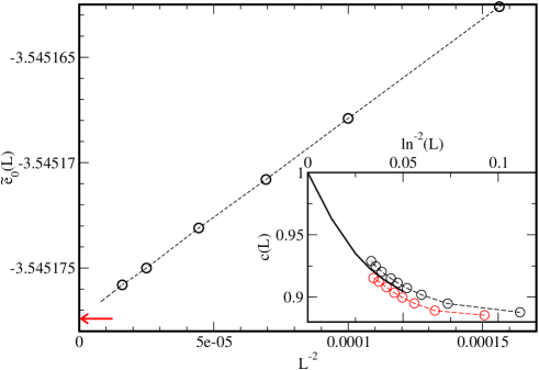
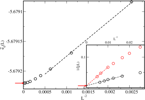
In order to get rid of the surface energy contribution we have calculated the bulk energy-density from the difference: e~0โ€‹(L)=[E0โ€‹(L+1)โˆ’E0โ€‹(Lโˆ’1)]/2subscript~๐‘’0๐ฟdelimited-[]subscript๐ธ0๐ฟ1subscript๐ธ0๐ฟ12{\tilde{e}}_{0}(L)=[E_{0}(L+1)-E_{0}(L-1)]/2, which has a finite-size correction term: +(ฯ€โ€‹cโ€‹v)/(24โ€‹L2)๐œ‹๐‘๐‘ฃ24superscript๐ฟ2+(\pi cv)/(24L^{2}). Indeed, as shown in Fig.1 the DMRG estimates for e~0โ€‹(L)subscript~๐‘’0๐ฟ{\tilde{e}}_{0}(L) approach the exact valuehamer : e0=4โ€‹lnโก4โˆ’2subscript๐‘’0442e_{0}=4\ln 4-2 within eight digit accuracy, furthermore the finite-size corrections are quadratic in 1/L1๐ฟ1/L. From the prefactor of the correction term we estimate an effective, size-dependent central charge in the range 0.88โˆ’0.940.880.940.88-0.94, for increasing L๐ฟL, see the inset of Fig.1. The variation of cโ€‹(L)๐‘๐ฟc(L) with the size is extremely slow, which is due to strong logarithmic correctionslogcorr . Our data are consistent with the asymptotic form: cโˆ’cโ€‹(L)โˆผlnโˆ’2โก(L)similar-to๐‘๐‘๐ฟsuperscript2๐ฟc-c(L)\sim\ln^{-2}(L), (see also in Ref.carlonigloi ) and we estimate c=1.02โ€‹(6)๐‘1.026c=1.02(6) in agreement with the known value c=1๐‘1c=1.

Refer to caption
Figure 1: (Color online) Ground-state energy per site of the Q=4๐‘„4Q=4-state model calculated by DMRG in finite chains, e~0โ€‹(L)subscript~๐‘’0๐ฟ{\tilde{e}}_{0}(L) (see text), as a function of Lโˆ’2superscript๐ฟ2L^{-2}. The arrow indicates the exact value. In the inset the effective central charge is shown versus lnโˆ’2โก(L)superscript2๐ฟ\ln^{-2}(L). Upper points: calculated with the use of the exact asymptotic value e0=4โ€‹lnโก4โˆ’2subscript๐‘’0442e_{0}=4\ln 4-2; lower points: calculated from two-point fits. The dashed and full lines are guide to the eye.

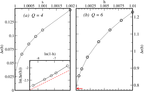
For the Q=6๐‘„6Q=6 model, for which the phase transition is of first order, the ground-state energy-density, e~0โ€‹(L)subscript~๐‘’0๐ฟ{\tilde{e}}_{0}(L) at the phase-transition point is shown in Fig.2. In this case the finite-size corrections are in the form โˆผ1/L2similar-toabsent1superscript๐ฟ2\sim 1/L^{2} up to L<ฮพ๐ฟ๐œ‰L<\xi, which turns to an exponential:

[e~0โ€‹(L)โˆ’e0]โˆผexpโก(โˆ’L/ฮพ),similar-todelimited-[]subscript~๐‘’0๐ฟsubscript๐‘’0๐ฟ๐œ‰[{\tilde{e}}_{0}(L)-e_{0}]\sim\exp(-L/\xi)\;, (10)

for L>ฮพ๐ฟ๐œ‰L>\xi. Here ฮพ๐œ‰\xi is the correlation length at the transition point, which is estimated through Eq.(10) and plotted in the inset of Fig.2.
Refer to caption
Figure 2: (Color online) Ground-state energy per site of the Q=6๐‘„6Q=6-state model calculated by DMRG in finite chains , e~0โ€‹(L)subscript~๐‘’0๐ฟ{\tilde{e}}_{0}(L) (see text), as a function of Lโˆ’2superscript๐ฟ2L^{-2}. The arrow indicates the exact value. In the inset the effective correlation length calculated through Eq.(10) is shown as a function of 1/L1๐ฟ1/L. (Lower points: calculated by two-point fits with the use of the exact asymptotic value of e0subscript๐‘’0e_{0}; upper points: calculated from three-point fits not using the exact asymptotic value of e0subscript๐‘’0e_{0}.) The analytical result in Eq.(8) is indicated by an arrow, the dashed lines are guide to the eye.

We have also calculated estimates for the latent heat defined by:

ฮ”โ€‹eโ€‹(h)=e~0โ€‹(h)โˆ’2โ€‹e~0โ€‹(hc)+e~0โ€‹(2โ€‹hcโˆ’h)hโˆ’hc,ฮ”๐‘’โ„Žsubscript~๐‘’0โ„Ž2subscript~๐‘’0subscriptโ„Ž๐‘subscript~๐‘’02subscriptโ„Ž๐‘โ„Žโ„Žsubscriptโ„Ž๐‘\Delta e(h)=\frac{{\tilde{e}}_{0}(h)-2{\tilde{e}}_{0}(h_{c})+{\tilde{e}}_{0}(2h_{c}-h)}{h-h_{c}}\;, (11)

by the DMRG method at a large value of L๐ฟL. Indeed in the limit Lโ†’โˆžโ†’๐ฟL\to\infty and hโ†’hcโ†’โ„Žsubscriptโ„Ž๐‘h\to h_{c} ฮ”โ€‹eโ€‹(h)ฮ”๐‘’โ„Ž\Delta e(h) corresponds to the latent heat in Eq.(7). Estimates for ฮ”โ€‹eโ€‹(h)ฮ”๐‘’โ„Ž\Delta e(h) are shown in Fig.3 for Q=4๐‘„4Q=4 (panel a) and for Q=6๐‘„6Q=6 (panel b). In the first case the effective latent heats tend to zero as hโ†’hcโ†’โ„Žsubscriptโ„Ž๐‘h\to h_{c}. As a matter of fact the effective latent heat at a second-order transition has a power-law dependence: ฮ”โ€‹eโ€‹(h)โˆผ(hโˆ’hc)1โˆ’ฮฑsimilar-toฮ”๐‘’โ„Žsuperscriptโ„Žsubscriptโ„Ž๐‘1๐›ผ\Delta e(h)\sim(h-h_{c})^{1-\alpha}, where ฮฑ๐›ผ\alpha is the critical exponent of the specific heat, being ฮฑ=2/3๐›ผ23\alpha=2/3 for the Q=4๐‘„4Q=4 Potts model. This type of scaling form applies for the numerical data, as seen in the inset Fig.3a. Here in a log-log plot ฮ”โ€‹eโ€‹(h)ฮ”๐‘’โ„Ž\Delta e(h) vs. hโˆ’1โ„Ž1h-1 is approximately linear and the slope is compatible with 1โˆ’ฮฑโ‰ˆ0.31๐›ผ0.31-\alpha\approx 0.3. (The relatively slow convergence is due to logarithmic corrections.logcorr ) On the contrary for the Q=6๐‘„6Q=6 model the effective latent heats in Fig.3b tend to a finite limiting value, and limhโ†’1ฮ”โ€‹eโ€‹(h)subscriptโ†’โ„Ž1ฮ”๐‘’โ„Ž\lim_{h\to 1}\Delta e(h) is compatible with the known analytical result in Eq.(7).
Refer to caption
Figure 3: (Color online) Estimates for the effective latent heat as defined in Eq.(11). Panel a: Q=4๐‘„4Q=4. In the inset the latent heat vs. (1-h) is shown in log-log plot. The slope of the dashed line is 0.30.30.3. Panel b: Q=6๐‘„6Q=6. The arrow indicates the analytical result in Eq.(7). The dashed and full lines are guide to the eye.

IV Entanglement entropy of the Potts chain

In the calculation of the entanglement entropy we separate the complete (open) system into two halves, such that ๐’œ๐’œ{\cal A} is represented by sites i=1,2,โ€ฆ,L/2๐‘–12โ€ฆ๐ฟ2i=1,2,\dots,L/2 and its complementer โ„ฌโ„ฌ{\cal B} consists of i=L/2+1,L/2+2,โ€ฆ,L๐‘–๐ฟ21๐ฟ22โ€ฆ๐ฟi=L/2+1,L/2+2,\dots,L. Using the definition in Eq.(1) the entanglement entropy is expressed with the eigenvalues of the reduced density matrix, ฮปjsubscript๐œ†๐‘—\lambda_{j} as: ๐’ฎA=โˆ’โˆ‘jฮปjโ€‹lnโกฮปjsubscript๐’ฎ๐ดsubscript๐‘—subscript๐œ†๐‘—subscript๐œ†๐‘—{\cal S}_{A}=-\sum_{j}\lambda_{j}\ln\lambda_{j}.

In the two limiting cases, h=0โ„Ž0h=0 and hโ†’โˆžโ†’โ„Žh\to\infty the entanglement entropy follows from a simple calculation. In the first case, h=0โ„Ž0h=0, the ground-state of the system is fully ferromagnetic and given in the representation of Eq.(5) as:

|ฮจ0โŸฉ=1Qโ€‹(|11โ€‹โ€ฆโ€‹1โŸฉ+|22โ€‹โ€ฆโ€‹2โŸฉ+โ‹ฏ+|Qโ€‹Qโ€‹โ€ฆโ€‹QโŸฉ).ketsubscriptฮจ01๐‘„ket11โ€ฆ1ket22โ€ฆ2โ‹ฏket๐‘„๐‘„โ€ฆ๐‘„|\Psi_{0}\rangle=\dfrac{1}{\sqrt{Q}}(|11\dots 1\rangle+|22\dots 2\rangle+\dots+|QQ\dots Q\rangle)\;. (12)

The reduced density matrix is diagonal and the non-vanishing eigenvalues are: ฮป1=ฮป2=โ€ฆโ€‹ฮปQ=1/Qsubscript๐œ†1subscript๐œ†2โ€ฆsubscript๐œ†๐‘„1๐‘„\lambda_{1}=\lambda_{2}=\dots\lambda_{Q}=1/Q, thus the entanglement entropy is: ๐’ฎAโ€‹(h=0)=lnโกQsubscript๐’ฎ๐ดโ„Ž0๐‘„{\cal S}_{A}(h=0)=\ln Q.

In the limit hโ†’โˆžโ†’โ„Žh\to\infty (or J=0๐ฝ0J=0) the system is fully paramagnetic and it is better to use the transformed basis in (6) in which the ground state is given by:

|ฮจ0โŸฉ=|1โ€ฒโ€‹1โ€ฒโ€‹โ€ฆโ€‹1โ€ฒโŸฉ,ketsubscriptฮจ0ketsuperscript1โ€ฒsuperscript1โ€ฒโ€ฆsuperscript1โ€ฒ|\Psi_{0}\rangle=|1^{\prime}1^{\prime}\dots 1^{\prime}\rangle\;, (13)

thus the entropy is: ๐’ฎAโ€‹(h=โˆž)=0subscript๐’ฎ๐ดโ„Ž0{\cal S}_{A}(h=\infty)=0.

For general values of hโ„Žh the entanglement entropy is calculated by different methods. For small finite chains, L=2๐ฟ2L=2 and 444 we make analytical calculations, in which Q๐‘„Q is a free parameter. For large systems, but for not too large Q๐‘„Q values, Q=4๐‘„4Q=4,666 and 888 we make numerical DMRG calculations. Finally, in the large-Q๐‘„Q limit we perform an 1/Q1๐‘„1/Q-expansion in leading order.

IV.1 Solution on finite chains for general values of Q๐‘„Q

In these calculations we calculate first the ground state of the system, for which we use the transformed basis in Eq.(6). As explained in the Appendix the eigenstates of โ„‹โ€ฒsuperscriptโ„‹โ€ฒ{\cal H^{\prime}} are separated into Q๐‘„Q disjoint sectors and the ground-state sector is separated further by symmetry. As a matter of fact the actual ground state is located in the subspace which has the maximal symmetry. This subspace has a finite dimension irrespective of the value of Q๐‘„Q and in the solution then Q๐‘„Q appears as a (not necessary integer) parametersolyompfeuty ; igloisolyom1 ; igloisolyom2 . Details of the calculation are explained in the Appendix, where - for simplicity - we choose J/Q=1๐ฝ๐‘„1J/Q=1 and with this parametrization the self-duality point is located at hc=1subscriptโ„Ž๐‘1h_{c}=1. For L=2๐ฟ2L=2 and L=4๐ฟ4L=4 we perform the complete calculation, for larger sizes we consider the large-Q๐‘„Q limit, so that our results are correct up to ๐’ชโ€‹(1/Q)๐’ช1๐‘„\mathcal{O}(1/Q).

IV.1.1 L=2๐ฟ2L=2

The ground state of the system is given by:

|ฮจ0โŸฉ=a1โ€‹|ฯ•1โŸฉ+1โˆ’a12โ€‹|ฯ•2โŸฉ,ketsubscriptฮจ0subscript๐‘Ž1ketsubscriptitalic-ฯ•11superscriptsubscript๐‘Ž12ketsubscriptitalic-ฯ•2|\Psi_{0}\rangle=a_{1}|\phi_{1}\rangle+\sqrt{1-a_{1}^{2}}|\phi_{2}\rangle\;, (14)

where |ฯ•1โŸฉketsubscriptitalic-ฯ•1|\phi_{1}\rangle and |ฯ•2โŸฉketsubscriptitalic-ฯ•2|\phi_{2}\rangle are defined in Eq.(24) and

1a12=1+[(hโˆ’1)โ€‹Q/2+1โˆ’Q2โ€‹(hโˆ’1)2+4โ€‹Qโ€‹h/2]2Qโˆ’1.1superscriptsubscript๐‘Ž121superscriptdelimited-[]โ„Ž1๐‘„21superscript๐‘„2superscriptโ„Ž124๐‘„โ„Ž22๐‘„1\dfrac{1}{a_{1}^{2}}=1+\dfrac{\left[(h-1)Q/2+1-\sqrt{Q^{2}(h-1)^{2}+4Qh}/2\right]^{2}}{Q-1}\;. (15)

The reduced density matrix is diagonal having the eigenvalues: ฮป1=a12subscript๐œ†1superscriptsubscript๐‘Ž12\lambda_{1}=a_{1}^{2}, ฮป2=(1โˆ’a12)/(Qโˆ’1)subscript๐œ†21superscriptsubscript๐‘Ž12๐‘„1\lambda_{2}=(1-a_{1}^{2})/(Q-1), ฮป3=(1โˆ’a12)/(Qโˆ’1)subscript๐œ†31superscriptsubscript๐‘Ž12๐‘„1\lambda_{3}=(1-a_{1}^{2})/(Q-1), โ€ฆโ€ฆ\dots, ฮปQ=(1โˆ’a12)/(Qโˆ’1)subscript๐œ†๐‘„1superscriptsubscript๐‘Ž12๐‘„1\lambda_{Q}=(1-a_{1}^{2})/(Q-1). Thus the entanglement entropy is given by:

๐’ฎL=2=โˆ’a12โ€‹lnโกa12โˆ’(1โˆ’a12)โ€‹lnโก(1โˆ’a12)+(1โˆ’a12)โ€‹lnโก(Qโˆ’1)subscript๐’ฎ๐ฟ2superscriptsubscript๐‘Ž12superscriptsubscript๐‘Ž121superscriptsubscript๐‘Ž121superscriptsubscript๐‘Ž121superscriptsubscript๐‘Ž12๐‘„1{\cal S}_{L=2}=-a_{1}^{2}\ln a_{1}^{2}-(1-a_{1}^{2})\ln(1-a_{1}^{2})+(1-a_{1}^{2})\ln(Q-1)\; (16)

At the critical point, h=1โ„Ž1h=1, we have a12=(1+Qโˆ’1/2)/2superscriptsubscript๐‘Ž121superscript๐‘„122a_{1}^{2}=(1+Q^{-1/2})/2 and the entanglement entropy for large-Q๐‘„Q is given by: ๐’ฎL=2โ€‹(h=1)โ‰ˆlnโกQ/2subscript๐’ฎ๐ฟ2โ„Ž1๐‘„2{\cal S}_{L=2}(h=1)\approx\ln Q/2, which is half of the value measured at h=0โ„Ž0h=0.

The derivative of the entanglement entropy at the transition point is divergent for large-Q๐‘„Q: โˆ‚๐’ฎL=2โˆ‚h|h=1โˆผโˆ’Q1/2similar-toevaluated-atsubscript๐’ฎ๐ฟ2โ„Žโ„Ž1superscript๐‘„12\left.\dfrac{\partial{\cal S}_{L=2}}{\partial h}\right|_{h=1}\sim-Q^{1/2}, and the cross-over regime between the large- and small-entropy regions has a size: ฮดโ€‹hL=2โˆผQโˆ’1/2similar-to๐›ฟsubscriptโ„Ž๐ฟ2superscript๐‘„12\delta h_{L=2}\sim Q^{-1/2}.

IV.1.2 L=4๐ฟ4L=4

The ground-state of the system is given by the linear combination:

|ฮจ0โŸฉ=โˆ‘i=17aiโ€‹|ฯ•iโŸฉketsubscriptฮจ0superscriptsubscript๐‘–17subscript๐‘Ž๐‘–ketsubscriptitalic-ฯ•๐‘–|\varPsi_{0}\rangle=\sum_{i=1}^{7}a_{i}|\phi_{i}\rangle (17)

where the basis vectors, |ฯ•iโŸฉketsubscriptitalic-ฯ•๐‘–|\phi_{i}\rangle, are defined in Eq.(26) and the parameters, aisubscript๐‘Ž๐‘–a_{i} are the components of the ground state eigenvector of the matrix in Eq.(27). The reduced density matrix, which is of Q2ร—Q2superscript๐‘„2superscript๐‘„2Q^{2}\times Q^{2} is split to Q๐‘„Q orthogonal sectors, among which (Qโˆ’1)๐‘„1(Q-1)-sectors are degenerate. The eigenvalues of the first matrix, Eisubscript๐ธ๐‘–E_{i}, i=1,2,โ€ฆ,Q๐‘–12โ€ฆ๐‘„i=1,2,\dots,Q are given by Eqs.(32) and (34), while the eigenvalues of the second matrix, Eยฏisubscriptยฏ๐ธ๐‘–\underline{E}_{i}, are in Eqs.(39), (41) and (43). The entanglement entropy is expressed in terms of ฮตiโ‰กEiโ€‹lnโกEisubscript๐œ€๐‘–subscript๐ธ๐‘–subscript๐ธ๐‘–\varepsilon_{i}\equiv E_{i}\ln E_{i} and ฮตยฏiโ‰กEยฏiโ€‹lnโกEยฏisubscriptยฏ๐œ€๐‘–subscriptยฏ๐ธ๐‘–subscriptยฏ๐ธ๐‘–\underline{\varepsilon}_{i}\equiv\underline{E}_{i}\ln\underline{E}_{i} as:

๐’ฎL=4=subscript๐’ฎ๐ฟ4absent\displaystyle{\cal S}_{L=4}= โˆ’\displaystyle- ฮต1โˆ’ฮต2โˆ’(Qโˆ’2)โ€‹ฮต3โˆ’subscript๐œ€1subscript๐œ€2limit-from๐‘„2subscript๐œ€3\displaystyle\varepsilon_{1}-\varepsilon_{2}-(Q-2)\varepsilon_{3}- (18)
โˆ’\displaystyle- (Qโˆ’1)โ€‹[โˆ’ฮตยฏ1โˆ’ฮตยฏ2โˆ’ฮตยฏQโˆ’(Qโˆ’3)โ€‹ฮตยฏ3]๐‘„1delimited-[]subscriptยฏ๐œ€1subscriptยฏ๐œ€2subscriptยฏ๐œ€๐‘„๐‘„3subscriptยฏ๐œ€3\displaystyle(Q-1)\left[-\underline{\varepsilon}_{1}-\underline{\varepsilon}_{2}-\underline{\varepsilon}_{Q}-(Q-3)\underline{\varepsilon}_{3}\right]

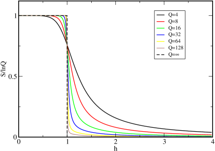
The entanglement entropy of the system as a function of hโ„Žh is shown in Fig.4 for different values of Q๐‘„Q. Being L๐ฟL finite, the entanglement entropy is analytical function of hโ„Žh, but its slope at hc=1subscriptโ„Ž๐‘1h_{c}=1 is increasing with Q๐‘„Q, asymptotically being โˆ‚๐’ฎL=4โˆ‚h|h=1โˆผโˆ’Q3/2similar-toevaluated-atsubscript๐’ฎ๐ฟ4โ„Žโ„Ž1superscript๐‘„32\left.\dfrac{\partial{\cal S}_{L=4}}{\partial h}\right|_{h=1}\sim-Q^{3/2}. Then the cross-over regime between the large- and small-entropy regions has a size: ฮดโ€‹hL=4โˆผQโˆ’3/2similar-to๐›ฟsubscriptโ„Ž๐ฟ4superscript๐‘„32\delta h_{L=4}\sim Q^{-3/2}.

Refer to caption
Figure 4: (Color online) Entanglement entropy of the Potts chain with L=4๐ฟ4L=4 sites for different values of Q๐‘„Q.

IV.1.3 Large-Q๐‘„Q limit

In the large-Q๐‘„Q limit the reduced density matrix is analyzed in leading order of 1/Q1๐‘„1/Q in the Appendix. The correction terms are found to be L๐ฟL-independent for Lโ‰ฅ4๐ฟ4L\geq 4 and the same holds for the entanglement entropy. This is given by:

๐’ฎโ‰ƒ2โ€‹[lnโก(Q2โ€‹(2โ€‹hโˆ’1)2)+1]Qโ€‹(2โ€‹hโˆ’1)2,h>1+ฮดโ€‹h,Qโ‰ซ1,formulae-sequencesimilar-to-or-equals๐’ฎ2delimited-[]superscript๐‘„2superscript2โ„Ž121๐‘„superscript2โ„Ž12formulae-sequenceโ„Ž1๐›ฟโ„Žmuch-greater-than๐‘„1{\cal S}\simeq\dfrac{2[\ln\left(Q^{2}(2h-1)^{2}\right)+1]}{Q(2h-1)^{2}},\quad h>1+\delta h,Q\gg 1\;, (19)

in the disordered phase and

๐’ฎโ‰ƒlnโกQโ€‹(1+Oโ€‹(1/Q2)),h<1โˆ’ฮดโ€‹h,Qโ‰ซ1,formulae-sequencesimilar-to-or-equals๐’ฎ๐‘„1๐‘‚1superscript๐‘„2formulae-sequenceโ„Ž1๐›ฟโ„Žmuch-greater-than๐‘„1{\cal S}\simeq\ln Q(1+O(1/Q^{2})),\quad h<1-\delta h,Q\gg 1\;, (20)

in the ordered phase. Here the cross-over value of the transverse field, ฮดโ€‹h๐›ฟโ„Ž\delta h is L๐ฟL-dependent and given in Eq.(48). In the thermodynamic limit ฮดโ€‹h๐›ฟโ„Ž\delta h goes to zero, thus the entanglement entropy is discontinuous in the large-Q๐‘„Q limit. Its jump at the transition point is given by:

ฮ”โ€‹๐’ฎ=lnโกQโ€‹[1โˆ’4Qโˆ’2Qโ€‹lnโกQ]+๐’ชโ€‹(1/Q2),ฮ”๐’ฎ๐‘„delimited-[]14๐‘„2๐‘„๐‘„๐’ช1superscript๐‘„2\Delta{\cal S}=\ln Q\left[1-\dfrac{4}{Q}-\dfrac{2}{Q\ln Q}\right]+\mathcal{O}(1/Q^{2})\;, (21)

which is decreasing with decreasing Q๐‘„Q, and at Qcโ‰ˆ5.2subscript๐‘„๐‘5.2Q_{c}\approx 5.2 this difference is vanishing. This leading order result is not too far from the exact criterion, Qc=4subscript๐‘„๐‘4Q_{c}=4.

IV.2 DMRG calculations

For finite values of Q๐‘„Q we have calculated the entanglement entropy numerically by the DMRG method. In these calculations we are focused to the neighbourhood of the transition point, which can not be treated successfully by (large- and small-hโ„Žh) expansion methods.

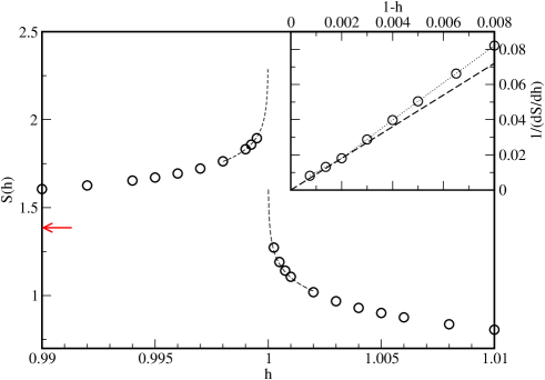
First, in Fig.5 we show results for the Q=4๐‘„4Q=4 model. In this case the transition is being of second order the entanglement entropy at the critical point is logarithmically divergent, as given in Eq.(2). In the vicinity of the transition point in Eq.(2) one should replace โ„“โ„“\ell with the correlation length, ฮพโˆผ|1โˆ’h|โˆ’ฮฝsimilar-to๐œ‰superscript1โ„Ž๐œˆ\xi\sim|1-h|^{-\nu}, thus the slope of the entanglement entropy has a divergence of the form:

โˆ‚๐’ฎโˆ‚hโ‰ˆโˆ’cโ€‹ฮฝ6โ€‹|1โˆ’h|โˆ’1.๐’ฎโ„Ž๐‘๐œˆ6superscript1โ„Ž1\frac{\partial\mathcal{S}}{\partial h}\approx-\frac{c\nu}{6}|1-h|^{-1}\;. (22)

The numerical results in the inset of Fig.5 are in agreement with this prediction, and the prefactor is compatible with the analytical value with c=1๐‘1c=1 and ฮฝ=2/3๐œˆ23\nu=2/3.

Refer to caption
Figure 5: (Color online) Entanglement entropy of the Q=4๐‘„4Q=4 model in the vicinity of the phase-transition calculated by DMRG. The arrow indicates the limiting value at h=0โ„Ž0h=0 and the dotted lines are guide to the eye. In the inset the inverse slope is plotted versus (1โˆ’h)1โ„Ž(1-h), see Eq.(22). Here the slope of the dashed straight line is 999, which corresponds to the analytical prediction.

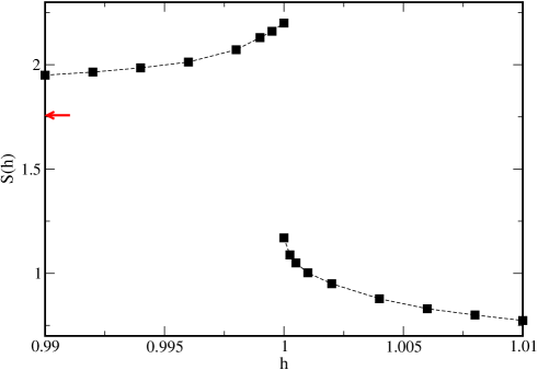
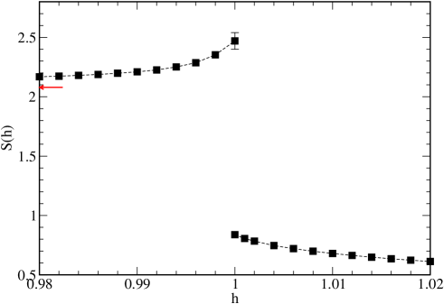
Results of a similar calculation for the Q=6๐‘„6Q=6 model are shown in Fig.6. In this case the entanglement entropy is monotonously increasing function of hโ‰ค1โ„Ž1h\leq 1 and the position of its (finite) maximum value is located at the transition point. Then, at h=1โ„Ž1h=1 it has a jump of ฮ”โ€‹๐’ฎ=1.04โ€‹(2)ฮ”๐’ฎ1.042\Delta{\cal S}=1.04(2), which is considerably larger than the first-order 1/Q1๐‘„1/Q result in Eq.(21). Thus the higher order terms are quite large for Q=6๐‘„6Q=6. In the paramagnetic phase the entanglement entropy is monotonously decreasing up to its limiting value ๐’ฎ=0๐’ฎ0\mathcal{S}=0, for large hโ„Žh.

We have also studied the Q=8๐‘„8Q=8 model, in which case the entanglement entropy has similar features as for Q=6๐‘„6Q=6, see in Fig.7. In this case the jump of the entropy at the transition point is found ฮ”โ€‹๐’ฎ=1.64โ€‹(8)ฮ”๐’ฎ1.648\Delta{\cal S}=1.64(8).

Refer to caption
Figure 6: (Color online) Entanglement entropy of the Q=6๐‘„6Q=6 model in the vicinity of the phase-transition calculated by DMRG. The arrow indicates the limiting value at h=0โ„Ž0h=0.
Refer to caption
Figure 7: (Color online) The same as in Fig.6 for the Q=8๐‘„8Q=8 model.

V Discussion

In this paper we have considered the ferromagnetic quantum Potts chain for Qโ‰ฅ4๐‘„4Q\geq 4 states and studied its entanglement properties close to the phase-transition point. Most of the results are numerical and obtained by the application of the DMRG method. To test the accuracy of the method first we have calculated some known properties of the model (ground-state energy-density, latent heat) and studied their finite-size scaling properties, both for second-order (Q=4๐‘„4Q=4) and for first-order (Q=6๐‘„6Q=6) transitions. In this way we have illustrated, how the finite-size scaling behaviour of these quantities at a first-order transition is modified, when the size of the system exceeds the equilibrium correlation length.

The entanglement entropy is found to show different scaling behavior at the transition point, depending on the order of the transition. For Q=4๐‘„4Q=4 at the second-order transition point the entanglement entropy is logarithmically divergent and the prefactor is observed in agreement with the prediction of conformal invariance. On the other hand for Q>4๐‘„4Q>4 at the first-order transition point the entanglement entropy stays finite, but develops a finite jump ฮ”โ€‹๐’ฎโ€‹(Q)>0ฮ”๐’ฎ๐‘„0\Delta{\cal S}(Q)>0. This jump is a monotonously increasing function of Q๐‘„Q and - according to our 1/Q1๐‘„1/Q expansion - it behaves as lnโกQ๐‘„\ln Q for large-Q๐‘„Q. It would be interesting to study by some method the behaviour of ฮ”โ€‹๐’ฎโ€‹(Q)ฮ”๐’ฎ๐‘„\Delta{\cal S}(Q) close to Q=4๐‘„4Q=4. Here one expects some kind of an essential singularity: ฮ”โ€‹๐’ฎโ€‹(Q)โˆผexpโก[โˆ’Aโ€‹(Qโˆ’4)โˆ’1/2]similar-toฮ”๐’ฎ๐‘„๐ดsuperscript๐‘„412\Delta{\cal S}(Q)\sim\exp[-A(Q-4)^{-1/2}], like in the latent heat.

To close our paper we mention a few related problems. For disordered chains the transition is of second-order, which is controlled by a so-called infinite disorder fixed pointdanielreview ; im . Then the entanglement entropy at the critical point follows the logarithmic scaling law in Eq.(2) with a so-called effective central charge given by: ceff=lnโกQ/2subscript๐‘eff๐‘„2c_{\rm eff}=\ln Q/2potts_dis . In the second problem we consider a single defect, which connects the two halves of the system, thus it is between sites i=L/2๐‘–๐ฟ2i=L/2 and i=L/2+1๐‘–๐ฟ21i=L/2+1 and given by ฮบโ€‹J๐œ…๐ฝ\kappa J. For the quantum Ising chain with Q=2๐‘„2Q=2 this problem has already been studied in different paperspeschel03 ; PeschelZhao ; Levine08 ; ISzL09 ; Eisler_Peschel10 ; CMV11 ; peschel12 and ฮบ๐œ…\kappa-dependent effective central charge has been obtained. This result is in agreement with the fact, that the defect represents a marginal perturbationipt for the Ising chain and the local critical behaviour is ฮบ๐œ…\kappa-dependent. In the second-order transition regime and for 2<Qโ‰ค42๐‘„42<Q\leq 4 the defect is a relevant perturbationipt , so that for 0<ฮบ<10๐œ…10<\kappa<1 it renormalizes to a cut and for ฮบ>1๐œ…1\kappa>1 it stays ordered at the transition point. In both cases the entanglement entropy is expected to have a finite, L๐ฟL-independent value (see related studies in Ref.ISzL09 ). In the first-order transition regime for Q>4๐‘„4Q>4 the previous reasoning does not hold and separate (numerical) investigations are needed to clarify the behaviour of the entanglement entropy. One further question is about the time-dependence of the entanglement entropy of the quantum Potts chain after a non-equilibrium process, such as a global or a local quantum quenchquench_rev . In the former case the couplings are changed uniformly and suddenly at t=0๐‘ก0t=0 and we are interested in the behaviour of ๐’ฎโ€‹(t)๐’ฎ๐‘ก{\cal S}(t) for t>0๐‘ก0t>0. Based on the quasi-particle picture a linearly increasing entanglement entropy, ๐’ฎโ€‹(t)โˆผtsimilar-to๐’ฎ๐‘ก๐‘ก{\cal S}(t)\sim t is expected asymptoticallyCC05 . The problem for local quench, when just the strength of a local coupling, say the coupling connecting the two subsystems is changed is more complicated and one can not use results from conformal invarianceEP07 ; CC07 ; stephan_dubail .

Acknowledgements.
This work was supported and funded by Kuwait University Research Grant No.[SP03/15]. The authors thank to Loรฏc Turban for cooperation in the early stages of the project.

*

Appendix A Solution on finite chains

In these calculations we use the transformed basis in (6) and make use of the fact that eigenstates of โ„‹โ€ฒsuperscriptโ„‹โ€ฒ{\cal H^{\prime}} are separated into Q๐‘„Q disjoint sectors. The ground-state sector is characterised by the state:

|ฯ•1โŸฉ=|1โ€ฒโ€‹1โ€ฒโ€‹โ€ฆโ€‹1โ€ฒโŸฉketsubscriptitalic-ฯ•1ketsuperscript1โ€ฒsuperscript1โ€ฒโ€ฆsuperscript1โ€ฒ|\phi_{1}\rangle=|1^{\prime}1^{\prime}\dots 1^{\prime}\rangle (23)

and the other QLโˆ’1โˆ’1superscript๐‘„๐ฟ11Q^{L-1}-1 states of the sector are obtained by acting โ„‹โ€ฒsuperscriptโ„‹โ€ฒ{\cal H^{\prime}} on |ฯ•1โŸฉketsubscriptitalic-ฯ•1|\phi_{1}\rangle. The other sectors are characterised with the states: |2โ€ฒ1โ€ฒโ€ฆ1โ€ฒโŸฉโŸฉ|2^{\prime}1^{\prime}\dots 1^{\prime}\rangle\rangle, |3โ€ฒ1โ€ฒโ€ฆ1โ€ฒโŸฉโŸฉ|3^{\prime}1^{\prime}\dots 1^{\prime}\rangle\rangle, โ€ฆโ€ฆ\dots,|Qโ€ฒ1โ€ฒโ€ฆ1โ€ฒโŸฉโŸฉ|Q^{\prime}1^{\prime}\dots 1^{\prime}\rangle\rangle, and these sectors are degenerate by symmetry. In the following we concentrate on the ground-state sector and determine its lowest state, which is thus the ground state of the system. Generally the ground state has the maximal symmetry, which helps us to construct it in a smaller basis set.

A.0.1 L=2๐ฟ2L=2

The ground state of the problem is in the sector |1โ€ฒโ€‹1โ€ฒโŸฉketsuperscript1โ€ฒsuperscript1โ€ฒ|1^{\prime}1^{\prime}\rangle having the maximal symmetry. This subspace is spanned by the vectors:

|ฯ•1โŸฉketsubscriptitalic-ฯ•1\displaystyle|\phi_{1}\rangle =\displaystyle= |1โ€ฒโ€‹1โ€ฒโŸฉketsuperscript1โ€ฒsuperscript1โ€ฒ\displaystyle|1^{\prime}1^{\prime}\rangle (24)
|ฯ•2โŸฉketsubscriptitalic-ฯ•2\displaystyle\;|\phi_{2}\rangle =\displaystyle= 1Qโˆ’1โ€‹[|2โ€ฒโ€‹Qโ€ฒโŸฉ+|3โ€ฒโ€‹(Qโˆ’1)โ€ฒโŸฉ+โ‹ฏ+|Qโ€ฒโ€‹2โ€ฒโŸฉ]1๐‘„1delimited-[]ketsuperscript2โ€ฒsuperscript๐‘„โ€ฒketsuperscript3โ€ฒsuperscript๐‘„1โ€ฒโ‹ฏketsuperscript๐‘„โ€ฒsuperscript2โ€ฒ\displaystyle\dfrac{1}{\sqrt{Q-1}}\left[|2^{\prime}Q^{\prime}\rangle+|3^{\prime}(Q-1)^{\prime}\rangle+\dots+|Q^{\prime}2^{\prime}\rangle\right]

We note that for L=2๐ฟ2L=2 - having periodic boundary conditions - there are two couplings between the two spins. Then the eigenvalue matrix corresponding to the symmetric subspace is given by:

HsymL=2=(โˆ’2โ€‹(Qโˆ’1)โ€‹hโˆ’2โ€‹Qโˆ’1โˆ’2โ€‹Qโˆ’12โ€‹hโˆ’2โ€‹(Qโˆ’2))superscriptsubscript๐ปsym๐ฟ22๐‘„1โ„Ž2๐‘„12๐‘„12โ„Ž2๐‘„2H_{\rm sym}^{L=2}=\left(\begin{array}[]{cc}-2(Q-1)h&-2\sqrt{Q-1}\\ -2\sqrt{Q-1}&2h-2(Q-2)\end{array}\right) (25)

and the eigenvector corresponding to the ground state has the components: a1subscript๐‘Ž1a_{1} and a2=1โˆ’a12subscript๐‘Ž21superscriptsubscript๐‘Ž12a_{2}=\sqrt{1-a_{1}^{2}}, which is given in Eq.(15).

A.0.2 L=4๐ฟ4L=4

In this case the symmetric subspace of the ground-state sector is spanned by the vectors:

|ฯ•1โŸฉketsubscriptitalic-ฯ•1\displaystyle|\phi_{1}\rangle =\displaystyle= |1โ€ฒโ€‹1โ€ฒโ€‹1โ€ฒโ€‹1โ€ฒโŸฉketsuperscript1โ€ฒsuperscript1โ€ฒsuperscript1โ€ฒsuperscript1โ€ฒ\displaystyle|1^{\prime}1^{\prime}1^{\prime}1^{\prime}\rangle
|ฯ•2โŸฉketsubscriptitalic-ฯ•2\displaystyle\;|\phi_{2}\rangle =\displaystyle= 14โ€‹Q1[|1โ€ฒ1โ€ฒ2โ€ฒQโ€ฒโŸฉ+|1โ€ฒ1โ€ฒ3โ€ฒ(Qโˆ’1)โ€ฒโŸฉ+โ‹ฏ+|1โ€ฒ1โ€ฒQโ€ฒ2โ€ฒโŸฉ+c.p.]\displaystyle\dfrac{1}{\sqrt{4Q_{1}}}\left[|1^{\prime}1^{\prime}2^{\prime}Q^{\prime}\rangle+|1^{\prime}1^{\prime}3^{\prime}(Q-1)^{\prime}\rangle+\dots+|1^{\prime}1^{\prime}Q^{\prime}2^{\prime}\rangle+c.p.\right]
|ฯ•3โŸฉketsubscriptitalic-ฯ•3\displaystyle\;|\phi_{3}\rangle =\displaystyle= 12โ€‹Q1[|1โ€ฒ2โ€ฒ1โ€ฒQโ€ฒโŸฉ+|1โ€ฒ3โ€ฒ1โ€ฒ(Qโˆ’1)โ€ฒโŸฉ+โ‹ฏ+|1โ€ฒQโ€ฒ1โ€ฒ2โ€ฒโŸฉ+c.p.]\displaystyle\dfrac{1}{\sqrt{2Q_{1}}}\left[|1^{\prime}2^{\prime}1^{\prime}Q^{\prime}\rangle+|1^{\prime}3^{\prime}1^{\prime}(Q-1)^{\prime}\rangle+\dots+|1^{\prime}Q^{\prime}1^{\prime}2^{\prime}\rangle+c.p.\right]
|ฯ•4โŸฉketsubscriptitalic-ฯ•4\displaystyle\;|\phi_{4}\rangle =\displaystyle= 1Q1โ€‹[|2โ€ฒโ€‹Qโ€ฒโ€‹2โ€ฒโ€‹Qโ€ฒโŸฉ+|3โ€ฒโ€‹(Qโˆ’1)โ€ฒโ€‹3โ€ฒโ€‹(Qโˆ’1)โ€ฒโŸฉ+โ‹ฏ+|Qโ€ฒโ€‹2โ€ฒโ€‹Qโ€ฒโ€‹2โ€ฒโŸฉ]1subscript๐‘„1delimited-[]ketsuperscript2โ€ฒsuperscript๐‘„โ€ฒsuperscript2โ€ฒsuperscript๐‘„โ€ฒketsuperscript3โ€ฒsuperscript๐‘„1โ€ฒsuperscript3โ€ฒsuperscript๐‘„1โ€ฒโ‹ฏketsuperscript๐‘„โ€ฒsuperscript2โ€ฒsuperscript๐‘„โ€ฒsuperscript2โ€ฒ\displaystyle\dfrac{1}{\sqrt{Q_{1}}}\left[|2^{\prime}Q^{\prime}2^{\prime}Q^{\prime}\rangle+|3^{\prime}(Q-1)^{\prime}3^{\prime}(Q-1)^{\prime}\rangle+\dots+|Q^{\prime}2^{\prime}Q^{\prime}2^{\prime}\rangle\right]
|ฯ•5โŸฉketsubscriptitalic-ฯ•5\displaystyle\;|\phi_{5}\rangle =\displaystyle= 14โ€‹Q1โ€‹Q2[|1โ€ฒ2โ€ฒ2โ€ฒ(Qโˆ’1)โ€ฒโŸฉ+|1โ€ฒ2โ€ฒ3โ€ฒ(Qโˆ’2)โ€ฒโŸฉ+โ‹ฏ+|1โ€ฒ2โ€ฒ(Qโˆ’1)โ€ฒ2โ€ฒโŸฉ\displaystyle\dfrac{1}{\sqrt{4Q_{1}Q_{2}}}\left[|1^{\prime}2^{\prime}2^{\prime}(Q-1)^{\prime}\rangle+|1^{\prime}2^{\prime}3^{\prime}(Q-2)^{\prime}\rangle+\dots+|1^{\prime}2^{\prime}(Q-1)^{\prime}2^{\prime}\rangle\right.
+\displaystyle+ |1โ€ฒ3โ€ฒ2โ€ฒ(Qโˆ’2)โ€ฒโŸฉ+โ‹ฏ+|1โ€ฒ3โ€ฒQโ€ฒQโ€ฒโŸฉ+โ‹ฏ+|1โ€ฒQโ€ฒ3โ€ฒQโ€ฒโŸฉ]\displaystyle\left.|1^{\prime}3^{\prime}2^{\prime}(Q-2)^{\prime}\rangle+\dots+|1^{\prime}3^{\prime}Q^{\prime}Q^{\prime}\rangle+\dots+|1^{\prime}Q^{\prime}3^{\prime}Q^{\prime}\rangle\right]
|ฯ•6โŸฉketsubscriptitalic-ฯ•6\displaystyle\;|\phi_{6}\rangle =\displaystyle= 12โ€‹Q1โ€‹Q2[|2โ€ฒQโ€ฒ3โ€ฒ(Qโˆ’1)โ€ฒโŸฉ+|2โ€ฒQโ€ฒ4โ€ฒ(Qโˆ’2)โ€ฒโŸฉโ‹ฏ+|2โ€ฒQโ€ฒQโ€ฒ2โ€ฒโŸฉ\displaystyle\dfrac{1}{\sqrt{2Q_{1}Q_{2}}}\left[|2^{\prime}Q^{\prime}3^{\prime}(Q-1)^{\prime}\rangle+|2^{\prime}Q^{\prime}4^{\prime}(Q-2)^{\prime}\rangle\dots+|2^{\prime}Q^{\prime}Q^{\prime}2^{\prime}\rangle\right.
+\displaystyle+ |3โ€ฒ(Qโˆ’1)โ€ฒ2โ€ฒQโ€ฒโŸฉ+โ‹ฏ+|3โ€ฒ(Qโˆ’1)โ€ฒQโ€ฒ2โ€ฒโŸฉ+โ‹ฏ+|Qโ€ฒ2โ€ฒ(Qโˆ’1)โ€ฒ3โ€ฒโŸฉ]\displaystyle\left.|3^{\prime}(Q-1)^{\prime}2^{\prime}Q^{\prime}\rangle+\dots+|3^{\prime}(Q-1)^{\prime}Q^{\prime}2^{\prime}\rangle+\dots+|Q^{\prime}2^{\prime}(Q-1)^{\prime}3^{\prime}\rangle\right]
|ฯ•7โŸฉketsubscriptitalic-ฯ•7\displaystyle\;|\phi_{7}\rangle =\displaystyle= 1Q1โ€‹Q2โ€‹Q3[|2โ€ฒ2โ€ฒ2โ€ฒ(Qโˆ’2)โ€ฒโŸฉ+|2โ€ฒ2โ€ฒ3โ€ฒ(Qโˆ’3)โ€ฒโŸฉโ‹ฏ+|2โ€ฒ2โ€ฒ(Qโˆ’2)โ€ฒ2โ€ฒโŸฉ\displaystyle\dfrac{1}{\sqrt{Q_{1}Q_{2}Q_{3}}}\left[|2^{\prime}2^{\prime}2^{\prime}(Q-2)^{\prime}\rangle+|2^{\prime}2^{\prime}3^{\prime}(Q-3)^{\prime}\rangle\dots+|2^{\prime}2^{\prime}(Q-2)^{\prime}2^{\prime}\rangle\right.
+\displaystyle+ |2โ€ฒ3โ€ฒ2โ€ฒ(Qโˆ’3)โ€ฒโŸฉโ‹ฏ+|2โ€ฒ3โ€ฒQโ€ฒ(Qโˆ’1)โ€ฒโŸฉ+โ‹ฏ+|Qโ€ฒQโ€ฒQโ€ฒ4โ€ฒโŸฉ]\displaystyle\left.|2^{\prime}3^{\prime}2^{\prime}(Q-3)^{\prime}\rangle\dots+|2^{\prime}3^{\prime}Q^{\prime}(Q-1)^{\prime}\rangle+\dots+|Q^{\prime}Q^{\prime}Q^{\prime}4^{\prime}\rangle\right] (26)

and the corresponding eigenvalue matrix is given by:

(โˆ’4โ€‹Q1โ€‹hโˆ’4โ€‹Q100000โˆ’4โ€‹Q1โˆ’2โ€‹Q2โ€‹hโˆ’Q2โˆ’8โˆ’2โˆ’2โ€‹Q2โˆ’2โ€‹Q200โˆ’8โˆ’2โ€‹hโ€‹Q20โˆ’8โ€‹Q2000โˆ’204โ€‹h0โˆ’8โ€‹Q200โˆ’2โ€‹Q2โˆ’8โ€‹Q20โˆ’Q4โ€‹hโˆ’2โ€‹Q2โˆ’8โˆ’4โ€‹Q30โˆ’2โ€‹Q20โˆ’8โ€‹Q2โˆ’84โ€‹hโˆ’2โ€‹Q3โˆ’8โ€‹Q30000โˆ’4โ€‹Q3โˆ’8โ€‹Q34โ€‹hโˆ’4โ€‹Q4)4subscript๐‘„1โ„Ž4subscript๐‘„1000004subscript๐‘„12subscript๐‘„2โ„Žsubscript๐‘„2822subscript๐‘„22subscript๐‘„20082โ„Žsubscript๐‘„208subscript๐‘„2000204โ„Ž08subscript๐‘„2002subscript๐‘„28subscript๐‘„20subscript๐‘„4โ„Ž2subscript๐‘„284subscript๐‘„302subscript๐‘„208subscript๐‘„284โ„Ž2subscript๐‘„38subscript๐‘„300004subscript๐‘„38subscript๐‘„34โ„Ž4subscript๐‘„4\left(\begin{array}[]{ccccccc}-4Q_{1}h&-\sqrt{4Q_{1}}&0&0&0&0&0\\ -\sqrt{4Q_{1}}&-2Q_{2}h-Q_{2}&-\sqrt{8}&-2&-2\sqrt{Q_{2}}&-\sqrt{2Q_{2}}&0\\ 0&-\sqrt{8}&-2hQ_{2}&0&-\sqrt{8Q_{2}}&0&0\\ 0&-2&0&4h&0&-\sqrt{8Q_{2}}&0\\ 0&-2\sqrt{Q_{2}}&-\sqrt{8Q_{2}}&0&-Q_{4}h-2Q_{2}&-\sqrt{8}&-4\sqrt{Q_{3}}\\ 0&-\sqrt{2Q_{2}}&0&-\sqrt{8Q_{2}}&-\sqrt{8}&4h-2Q_{3}&-\sqrt{8Q_{3}}\\ 0&0&0&0&-4\sqrt{Q_{3}}&-\sqrt{8Q_{3}}&4h-4Q_{4}\par\end{array}\right) (27)

Here and in the following we use the short-hand notation, Qkโ‰กQโˆ’ksubscript๐‘„๐‘˜๐‘„๐‘˜Q_{k}\equiv Q-k, for k=1,2,3๐‘˜123k=1,2,3 and 444. The matrix-elemets of the reduced density matrix, ฯAโ€‹(s1โ€ฒโ€‹s2โ€ฒ,s~1โ€ฒโ€‹s~2โ€ฒ)subscript๐œŒ๐ดsubscriptsuperscript๐‘ โ€ฒ1subscriptsuperscript๐‘ โ€ฒ2subscriptsuperscript~๐‘ โ€ฒ1subscriptsuperscript~๐‘ โ€ฒ2\mathbf{\rho}_{A}(s^{\prime}_{1}s^{\prime}_{2},\tilde{s}^{\prime}_{1}\tilde{s}^{\prime}_{2}), are non-zero only for states with s1โ€ฒ+s2โ€ฒโˆ’(s~1โ€ฒ+s~2โ€ฒ))=0,modQs^{\prime}_{1}+s^{\prime}_{2}-(\tilde{s}^{\prime}_{1}+\tilde{s}^{\prime}_{2}))=0,{\rm mod}~{}Q. The reduced density matrix is devided into Q๐‘„Q orthogonal sectors. The first sector contains matrix-elements between the states: 11,2โ€‹Q,3โ€‹(Qโˆ’1),โ€ฆ,Qโ€‹2112๐‘„3๐‘„1โ€ฆ๐‘„211,2Q,3(Q-1),\dots,Q2. In the second sector there are matrix-elements between the states: 12,21,3โ€‹Q,โ€ฆ,Qโ€‹312213๐‘„โ€ฆ๐‘„312,21,3Q,\dots,Q3. The n๐‘›n-th sector is characterized by the states: 1โ€‹n,nโ€‹1,2โ€‹(nโˆ’1),โ€ฆ,Qโ€‹(n+1)1๐‘›๐‘›12๐‘›1โ€ฆ๐‘„๐‘›11n,n1,2(n-1),\dots,Q(n+1). These latter (Qโˆ’1)๐‘„1(Q-1) sectors are degenerate due to symmetry. In the following we solve the eigenvalue problems of the different sectors.

111111 sector

The Qร—Q๐‘„๐‘„Q\times Q eigenvalue matrix in this sector is given in the form:

(accccโ€ฆccbdddโ€ฆdcdbddโ€ฆdcddbdโ€ฆdcdddbโ€ฆdโ‹ฎโ‹ฎโ‹ฎโ‹ฎโ‹ฎโ‹ฑโ‹ฎcddddโ€ฆd)๐‘Ž๐‘๐‘๐‘๐‘โ€ฆ๐‘๐‘๐‘๐‘‘๐‘‘๐‘‘โ€ฆ๐‘‘๐‘๐‘‘๐‘๐‘‘๐‘‘โ€ฆ๐‘‘๐‘๐‘‘๐‘‘๐‘๐‘‘โ€ฆ๐‘‘๐‘๐‘‘๐‘‘๐‘‘๐‘โ€ฆ๐‘‘โ‹ฎโ‹ฎโ‹ฎโ‹ฎโ‹ฎโ‹ฑโ‹ฎ๐‘๐‘‘๐‘‘๐‘‘๐‘‘โ€ฆ๐‘‘\left(\begin{array}[]{ccccccc}a&c&c&c&c&\dots&c\\ c&b&d&d&d&\dots&d\\ c&d&b&d&d&\dots&d\\ c&d&d&b&d&\dots&d\\ c&d&d&d&b&\dots&d\\ \vdots&\vdots&\vdots&\vdots&\vdots&\ddots&\vdots\\ c&d&d&d&d&\dots&d\end{array}\right) (28)

with

a๐‘Ž\displaystyle a =\displaystyle= a12+a22/4superscriptsubscript๐‘Ž12superscriptsubscript๐‘Ž224\displaystyle a_{1}^{2}+a_{2}^{2}/4
b๐‘\displaystyle\;b =\displaystyle= 14โ€‹Q1โ€‹(a22+4โ€‹a42+2โ€‹a62)14subscript๐‘„1superscriptsubscript๐‘Ž224superscriptsubscript๐‘Ž422superscriptsubscript๐‘Ž62\displaystyle\dfrac{1}{4Q_{1}}(a_{2}^{2}+4a_{4}^{2}+2a_{6}^{2}) (29)
c๐‘\displaystyle\;c =\displaystyle= a1โ€‹a22โ€‹Q1+a2โ€‹a42โ€‹Q1+a2โ€‹a6โ€‹Q28โ€‹Q1subscript๐‘Ž1subscript๐‘Ž22subscript๐‘„1subscript๐‘Ž2subscript๐‘Ž42subscript๐‘„1subscript๐‘Ž2subscript๐‘Ž6subscript๐‘„28subscript๐‘„1\displaystyle\dfrac{a_{1}a_{2}}{2\sqrt{Q_{1}}}+\dfrac{a_{2}a_{4}}{2Q_{1}}+\dfrac{a_{2}a_{6}\sqrt{Q_{2}}}{\sqrt{8}Q_{1}}
d๐‘‘\displaystyle\;d =\displaystyle= a224โ€‹Q1+2โ€‹a4โ€‹a6Q1โ€‹Q2+a62โ€‹Q32โ€‹Q1โ€‹Q2.superscriptsubscript๐‘Ž224subscript๐‘„12subscript๐‘Ž4subscript๐‘Ž6subscript๐‘„1subscript๐‘„2superscriptsubscript๐‘Ž62subscript๐‘„32subscript๐‘„1subscript๐‘„2\displaystyle\dfrac{a_{2}^{2}}{4Q_{1}}+\dfrac{\sqrt{2}a_{4}a_{6}}{Q_{1}\sqrt{Q_{2}}}+\dfrac{a_{6}^{2}Q_{3}}{2Q_{1}Q_{2}}\;.

Two eigenvalues are given in the space of the vectors:

ฮจ1subscriptฮจ1\displaystyle\varPsi_{1} =\displaystyle= ฯ†1subscript๐œ‘1\displaystyle\varphi_{1}
ฮจ2subscriptฮจ2\displaystyle\;\varPsi_{2} =\displaystyle= 1Q1โ€‹[ฯ†2+ฯ†3+โ‹ฏ+ฯ†Q]1subscript๐‘„1delimited-[]subscript๐œ‘2subscript๐œ‘3โ‹ฏsubscript๐œ‘๐‘„\displaystyle\dfrac{1}{\sqrt{Q_{1}}}\left[\varphi_{2}+\varphi_{3}+\dots+\varphi_{Q}\right] (30)

having an eigenvalue matrix:

(acโ€‹Q1cโ€‹Q1b+dโ€‹Q2)๐‘Ž๐‘subscript๐‘„1๐‘subscript๐‘„1๐‘๐‘‘subscript๐‘„2\left(\begin{array}[]{cc}a&c\sqrt{Q_{1}}\\ c\sqrt{Q_{1}}&b+dQ_{2}\end{array}\right) (31)

with the eigenvalues:

E1,2=a+b+dโ€‹Q22ยฑ[aโˆ’bโˆ’dโ€‹Q22]2+c2โ€‹Q1subscript๐ธ12plus-or-minus๐‘Ž๐‘๐‘‘subscript๐‘„22superscriptdelimited-[]๐‘Ž๐‘๐‘‘subscript๐‘„222superscript๐‘2subscript๐‘„1E_{1,2}=\dfrac{a+b+dQ_{2}}{2}\pm\sqrt{\left[\dfrac{a-b-dQ_{2}}{2}\right]^{2}+c^{2}Q_{1}} (32)

The other (Qโˆ’2)๐‘„2(Q-2) eigenvalues are degenerate. The corresponding eigenvectors are given in the form:

ฮฆ3subscriptฮฆ3\displaystyle\varPhi_{3} =\displaystyle= 1Q1โ€‹[ฯ†2+ฮทโ€‹ฯ†3+ฮท2โ€‹ฯ†3+โ‹ฏ+ฮทQ2โ€‹ฯ†Q]1subscript๐‘„1delimited-[]subscript๐œ‘2๐œ‚subscript๐œ‘3superscript๐œ‚2subscript๐œ‘3โ‹ฏsuperscript๐œ‚subscript๐‘„2subscript๐œ‘๐‘„\displaystyle\dfrac{1}{\sqrt{Q_{1}}}\left[\varphi_{2}+\eta\varphi_{3}+\eta^{2}\varphi_{3}+\dots+\eta^{Q_{2}}\varphi_{Q}\right]
ฮฆ4subscriptฮฆ4\displaystyle\varPhi_{4} =\displaystyle= 1Q1โ€‹[ฯ†2+ฮท2โ€‹ฯ†3+ฮท4โ€‹ฯ†3+โ‹ฏ+ฮท2โ€‹Q2โ€‹ฯ†Q]1subscript๐‘„1delimited-[]subscript๐œ‘2superscript๐œ‚2subscript๐œ‘3superscript๐œ‚4subscript๐œ‘3โ‹ฏsuperscript๐œ‚2subscript๐‘„2subscript๐œ‘๐‘„\displaystyle\dfrac{1}{\sqrt{Q_{1}}}\left[\varphi_{2}+\eta^{2}\varphi_{3}+\eta^{4}\varphi_{3}+\dots+\eta^{2Q_{2}}\varphi_{Q}\right]
โ‹ฎโ‹ฎ\displaystyle\vdots
ฮฆQsubscriptฮฆ๐‘„\displaystyle\varPhi_{Q} =\displaystyle= 1Q1โ€‹[ฯ†2+ฮทQ2โ€‹ฯ†3+ฮท2โ€‹Q2โ€‹ฯ†3+โ‹ฏ+ฮทQ22โ€‹ฯ†Q]1subscript๐‘„1delimited-[]subscript๐œ‘2superscript๐œ‚subscript๐‘„2subscript๐œ‘3superscript๐œ‚2subscript๐‘„2subscript๐œ‘3โ‹ฏsuperscript๐œ‚superscriptsubscript๐‘„22subscript๐œ‘๐‘„\displaystyle\dfrac{1}{\sqrt{Q_{1}}}\left[\varphi_{2}+\eta^{Q_{2}}\varphi_{3}+\eta^{2Q_{2}}\varphi_{3}+\dots+\eta^{Q_{2}^{2}}\varphi_{Q}\right]

with ฮท=expโก(2โ€‹ฯ€โ€‹ฤฑQโˆ’1)๐œ‚2๐œ‹italic-ฤฑ๐‘„1\eta=\exp\left(\dfrac{2\pi\imath}{Q-1}\right). The eigenvalues are:

E3=E4=โ‹ฏ=EQ=bโˆ’dsubscript๐ธ3subscript๐ธ4โ‹ฏsubscript๐ธ๐‘„๐‘๐‘‘E_{3}=E_{4}=\dots=E_{Q}=b-d (34)

121212 sector

The Qร—Q๐‘„๐‘„Q\times Q eigenvalue matrix in this sector is given in the form:

(ฮฑฮณฮดฮดฮดโ€ฆฮดฮณฮฑฮดฮดฮดโ€ฆฮดฮดฮดฮฒฮตฮตโ€ฆฮตฮดฮดฮตฮฒฮตโ€ฆฮตฮดฮดฮตฮตฮฒโ€ฆฮตโ‹ฎโ‹ฎโ‹ฎโ‹ฎโ‹ฎโ‹ฑโ‹ฎฮดฮดฮตฮตฮตโ€ฆฮฒ)๐›ผ๐›พ๐›ฟ๐›ฟ๐›ฟโ€ฆ๐›ฟ๐›พ๐›ผ๐›ฟ๐›ฟ๐›ฟโ€ฆ๐›ฟ๐›ฟ๐›ฟ๐›ฝ๐œ€๐œ€โ€ฆ๐œ€๐›ฟ๐›ฟ๐œ€๐›ฝ๐œ€โ€ฆ๐œ€๐›ฟ๐›ฟ๐œ€๐œ€๐›ฝโ€ฆ๐œ€โ‹ฎโ‹ฎโ‹ฎโ‹ฎโ‹ฎโ‹ฑโ‹ฎ๐›ฟ๐›ฟ๐œ€๐œ€๐œ€โ€ฆ๐›ฝ\left(\begin{array}[]{ccccccc}\alpha&\gamma&\delta&\delta&\delta&\dots&\delta\\ \gamma&\alpha&\delta&\delta&\delta&\dots&\delta\\ \delta&\delta&\beta&\varepsilon&\varepsilon&\dots&\varepsilon\\ \delta&\delta&\varepsilon&\beta&\varepsilon&\dots&\varepsilon\\ \delta&\delta&\varepsilon&\varepsilon&\beta&\dots&\varepsilon\\ \vdots&\vdots&\vdots&\vdots&\vdots&\ddots&\vdots\\ \delta&\delta&\varepsilon&\varepsilon&\varepsilon&\dots&\beta\end{array}\right) (35)

with

ฮฑ๐›ผ\displaystyle\alpha =\displaystyle= 14โ€‹Q1โ€‹(a22+2โ€‹a32+a52)14subscript๐‘„1superscriptsubscript๐‘Ž222superscriptsubscript๐‘Ž32superscriptsubscript๐‘Ž52\displaystyle\dfrac{1}{4Q_{1}}(a_{2}^{2}+2a_{3}^{2}+a_{5}^{2})
ฮฒ๐›ฝ\displaystyle\;\beta =\displaystyle= 12โ€‹Q1โ€‹Q2โ€‹(a52+a62+2โ€‹a72)12subscript๐‘„1subscript๐‘„2superscriptsubscript๐‘Ž52superscriptsubscript๐‘Ž622superscriptsubscript๐‘Ž72\displaystyle\dfrac{1}{2Q_{1}Q_{2}}(a_{5}^{2}+a_{6}^{2}+2a_{7}^{2})
ฮณ๐›พ\displaystyle\;\gamma =\displaystyle= a2โ€‹a32โ€‹Q1+a524โ€‹Q1subscript๐‘Ž2subscript๐‘Ž32subscript๐‘„1superscriptsubscript๐‘Ž524subscript๐‘„1\displaystyle\dfrac{a_{2}a_{3}}{\sqrt{2}Q_{1}}+\dfrac{a_{5}^{2}}{4Q_{1}}
ฮด๐›ฟ\displaystyle\;\delta =\displaystyle= a2โ€‹a54โ€‹Q1โ€‹Q2+a3โ€‹a58โ€‹Q1โ€‹Q2+a5โ€‹a68โ€‹Q1โ€‹Q2+a5โ€‹a7โ€‹Q32โ€‹Q1โ€‹Q2subscript๐‘Ž2subscript๐‘Ž54subscript๐‘„1subscript๐‘„2subscript๐‘Ž3subscript๐‘Ž58subscript๐‘„1subscript๐‘„2subscript๐‘Ž5subscript๐‘Ž68subscript๐‘„1subscript๐‘„2subscript๐‘Ž5subscript๐‘Ž7subscript๐‘„32subscript๐‘„1subscript๐‘„2\displaystyle\dfrac{a_{2}a_{5}}{4Q_{1}\sqrt{Q_{2}}}+\dfrac{a_{3}a_{5}}{\sqrt{8}Q_{1}\sqrt{Q_{2}}}+\dfrac{a_{5}a_{6}}{\sqrt{8}Q_{1}Q_{2}}+\dfrac{a_{5}a_{7}\sqrt{Q_{3}}}{2Q_{1}Q_{2}}
ฮต๐œ€\displaystyle\;\varepsilon =\displaystyle= a522โ€‹Q1โ€‹Q2+a6โ€‹a7โ€‹2Q1โ€‹Q2โ€‹Q3+a72โ€‹Q4Q1โ€‹Q2โ€‹Q3.superscriptsubscript๐‘Ž522subscript๐‘„1subscript๐‘„2subscript๐‘Ž6subscript๐‘Ž72subscript๐‘„1subscript๐‘„2subscript๐‘„3superscriptsubscript๐‘Ž72subscript๐‘„4subscript๐‘„1subscript๐‘„2subscript๐‘„3\displaystyle\dfrac{a_{5}^{2}}{2Q_{1}Q_{2}}+\dfrac{a_{6}a_{7}\sqrt{2}}{Q_{1}Q_{2}\sqrt{Q_{3}}}+\dfrac{a_{7}^{2}Q_{4}}{Q_{1}Q_{2}Q_{3}}\;. (36)

Two eigenvalues are given in the space of the vectors:

ฮจยฏ1subscriptยฏฮจ1\displaystyle\underline{\varPsi}_{1} =\displaystyle= 12โ€‹[ฯ†ยฏ1+ฯ†ยฏ2]12delimited-[]subscriptยฏ๐œ‘1subscriptยฏ๐œ‘2\displaystyle\dfrac{1}{\sqrt{2}}\left[\underline{\varphi}_{1}+\underline{\varphi}_{2}\right]
ฮจยฏ2subscriptยฏฮจ2\displaystyle\;\underline{\varPsi}_{2} =\displaystyle= 1Q2โ€‹[ฯ†ยฏ3+ฯ†ยฏ4+โ‹ฏ+ฯ†ยฏQ]1subscript๐‘„2delimited-[]subscriptยฏ๐œ‘3subscriptยฏ๐œ‘4โ‹ฏsubscriptยฏ๐œ‘๐‘„\displaystyle\dfrac{1}{\sqrt{Q_{2}}}\left[\underline{\varphi}_{3}+\underline{\varphi}_{4}+\dots+\underline{\varphi}_{Q}\right] (37)

having an eigenvalue matrix:

(ฮฑ+ฮณฮดโ€‹2โ€‹Q2ฮดโ€‹2โ€‹Q2ฮฒ+ฮตโ€‹Q3)๐›ผ๐›พ๐›ฟ2subscript๐‘„2๐›ฟ2subscript๐‘„2๐›ฝ๐œ€subscript๐‘„3\left(\begin{array}[]{cc}\alpha+\gamma&\delta\sqrt{2Q_{2}}\\ \delta\sqrt{2Q_{2}}&\beta+\varepsilon Q_{3}\end{array}\right) (38)

with the eigenvalues:

Eยฏ1,2subscriptยฏ๐ธ12\displaystyle\underline{E}_{1,2} =\displaystyle= ฮฑ+ฮณ+ฮฒ+ฮตโ€‹Q32๐›ผ๐›พ๐›ฝ๐œ€subscript๐‘„32\displaystyle\dfrac{\alpha+\gamma+\beta+\varepsilon Q_{3}}{2} (39)
ยฑplus-or-minus\displaystyle\pm [ฮฑ+ฮณโˆ’ฮฒโˆ’ฮตโ€‹Q32]2+ฮด2โ€‹2โ€‹Q2superscriptdelimited-[]๐›ผ๐›พ๐›ฝ๐œ€subscript๐‘„322superscript๐›ฟ22subscript๐‘„2\displaystyle\sqrt{\left[\dfrac{\alpha+\gamma-\beta-\varepsilon Q_{3}}{2}\right]^{2}+\delta^{2}2Q_{2}}

Another (Qโˆ’3)๐‘„3(Q-3) eigenvalues are degenerate. The corresponding eigenvectors are given in the form:

ฮฆยฏ3subscriptยฏฮฆ3\displaystyle\underline{\varPhi}_{3} =\displaystyle= 1Q2โ€‹[ฯ†ยฏ3+ฮทยฏโ€‹ฯ†ยฏ4+ฮทยฏ2โ€‹ฯ†ยฏ5+โ‹ฏ+ฮทยฏQ3โ€‹ฯ†ยฏQ]1subscript๐‘„2delimited-[]subscriptยฏ๐œ‘3ยฏ๐œ‚subscriptยฏ๐œ‘4superscriptยฏ๐œ‚2subscriptยฏ๐œ‘5โ‹ฏsuperscriptยฏ๐œ‚subscript๐‘„3subscriptยฏ๐œ‘๐‘„\displaystyle\dfrac{1}{\sqrt{Q_{2}}}\left[\underline{\varphi}_{3}+\underline{\eta}\underline{\varphi}_{4}+\underline{\eta}^{2}\underline{\varphi}_{5}+\dots+\underline{\eta}^{Q_{3}}\underline{\varphi}_{Q}\right]
ฮฆยฏ4subscriptยฏฮฆ4\displaystyle\underline{\varPhi}_{4} =\displaystyle= 1Q2โ€‹[ฯ†ยฏ3+ฮท2โ€‹ฯ†ยฏ4+ฮท4โ€‹ฯ†ยฏ5+โ‹ฏ+ฮท2โ€‹Q3โ€‹ฯ†ยฏQ]1subscript๐‘„2delimited-[]subscriptยฏ๐œ‘3superscript๐œ‚2subscriptยฏ๐œ‘4superscript๐œ‚4subscriptยฏ๐œ‘5โ‹ฏsuperscript๐œ‚2subscript๐‘„3subscriptยฏ๐œ‘๐‘„\displaystyle\dfrac{1}{\sqrt{Q_{2}}}\left[\underline{\varphi}_{3}+\eta^{2}\underline{\varphi}_{4}+\eta^{4}\underline{\varphi}_{5}+\dots+\eta^{2Q_{3}}\underline{\varphi}_{Q}\right]
โ€ฆโ€ฆ\displaystyle\dots
ฮฆยฏQโˆ’1subscriptยฏฮฆ๐‘„1\displaystyle\underline{\varPhi}_{Q-1} =\displaystyle= 1Q2โ€‹[ฯ†ยฏ3+ฮทยฏQ3โ€‹ฯ†ยฏ4+ฮทยฏ2โ€‹Q3โ€‹ฯ†ยฏ5+โ‹ฏ+ฮทยฏQ32โ€‹ฯ†ยฏQ]1subscript๐‘„2delimited-[]subscriptยฏ๐œ‘3superscriptยฏ๐œ‚subscript๐‘„3subscriptยฏ๐œ‘4superscriptยฏ๐œ‚2subscript๐‘„3subscriptยฏ๐œ‘5โ‹ฏsuperscriptยฏ๐œ‚superscriptsubscript๐‘„32subscriptยฏ๐œ‘๐‘„\displaystyle\dfrac{1}{\sqrt{Q_{2}}}\left[\underline{\varphi}_{3}+\underline{\eta}^{Q_{3}}\underline{\varphi}_{4}+\underline{\eta}^{2Q_{3}}\underline{\varphi}_{5}+\dots+\underline{\eta}^{Q_{3}^{2}}\underline{\varphi}_{Q}\right]

with ฮทยฏ=expโก(2โ€‹ฯ€โ€‹ฤฑQโˆ’2)ยฏ๐œ‚2๐œ‹italic-ฤฑ๐‘„2\underline{\eta}=\exp\left(\dfrac{2\pi\imath}{Q-2}\right). The eigenvalues are:

Eยฏ3=Eยฏ4=โ‹ฏ=EยฏQโˆ’1=ฮฒโˆ’ฮตsubscriptยฏ๐ธ3subscriptยฏ๐ธ4โ‹ฏsubscriptยฏ๐ธ๐‘„1๐›ฝ๐œ€\underline{E}_{3}=\underline{E}_{4}=\dots=\underline{E}_{Q-1}=\beta-\varepsilon (41)

Finally, last eigenvector is given by:

ฮฆยฏQ=12โ€‹[ฯ†ยฏ1โˆ’ฯ†ยฏ2]subscriptยฏฮฆ๐‘„12delimited-[]subscriptยฏ๐œ‘1subscriptยฏ๐œ‘2\underline{\varPhi}_{Q}=\dfrac{1}{\sqrt{2}}\left[\underline{\varphi}_{1}-\underline{\varphi}_{2}\right] (42)

with the eigenvalue:

EยฏQ=ฮฑโˆ’ฮณsubscriptยฏ๐ธ๐‘„๐›ผ๐›พ\underline{E}_{Q}=\alpha-\gamma (43)

The entanglement entropy of the system is expressed in terms of the eigenvalues, Eisubscript๐ธ๐‘–E_{i} and Eยฏisubscriptยฏ๐ธ๐‘–\underline{E}_{i} and given in Eq.(IV.1.2).

A.0.3 Large-Q๐‘„Q limit

For large-Q๐‘„Q we consider the leading behaviour up to 1/Q1๐‘„1/Q, when the matrix-elements of the reduced density matrix are different in the disordered and in the ordered phase, respectively. We start with the analysis of the results of the previous subsection for the L=4๐ฟ4L=4 chain.

In the disordered regime, h>1+ฮดโ€‹hโ„Ž1๐›ฟโ„Žh>1+\delta h, in leading order the following matrix-elements are non-zero:

a๐‘Ž\displaystyle a =\displaystyle= 1โˆ’3Qโ€‹(2โ€‹hโˆ’1)2,b=d=ฮฑ=1Q2โ€‹(2โ€‹hโˆ’1)213๐‘„superscript2โ„Ž12๐‘๐‘‘๐›ผ1superscript๐‘„2superscript2โ„Ž12\displaystyle 1-\dfrac{3}{Q(2h-1)^{2}},\quad b=d=\alpha=\dfrac{1}{Q^{2}(2h-1)^{2}}
c๐‘\displaystyle\;c =\displaystyle= 1Qโ€‹(2โ€‹hโˆ’1)1๐‘„2โ„Ž1\displaystyle\dfrac{1}{Q(2h-1)}\; (44)

and the leading contribution to the entropy is given in Eq.(19).

In the ordered regime, h<1โˆ’ฮดโ€‹hโ„Ž1๐›ฟโ„Žh<1-\delta h, the non-zero matrix-elements in leading order are the following:

ฮฑ๐›ผ\displaystyle\alpha =\displaystyle= ฮณ=4Q2โ€‹(2โˆ’h)2,ฮด=2Q2โ€‹(2โˆ’h),formulae-sequence๐›พ4superscript๐‘„2superscript2โ„Ž2๐›ฟ2superscript๐‘„22โ„Ž\displaystyle\gamma=\dfrac{4}{Q^{2}(2-h)^{2}},\quad\delta=\dfrac{2}{Q^{2}(2-h)}, (45)
b๐‘\displaystyle\;b =\displaystyle= d=1Q2,ฮฒ=ฮต=1Q2โ€‹[1โˆ’1Qโ€‹(8(2โˆ’h)2+1)]formulae-sequence๐‘‘1superscript๐‘„2๐›ฝ๐œ€1superscript๐‘„2delimited-[]11๐‘„8superscript2โ„Ž21\displaystyle d=\dfrac{1}{Q^{2}},\quad\beta=\varepsilon=\dfrac{1}{Q^{2}}\left[1-\dfrac{1}{Q}\left(\dfrac{8}{(2-h)^{2}}+1\right)\right]\;

and the leading contribution to the entropy is given in Eq.(20).

Finally, at the phase-transition point, h=1โ„Ž1h=1, the matrix-elements in leading order are a=1/2๐‘Ž12a=1/2, ฮฒ=1/[(qโˆ’1)โ€‹(qโˆ’2)]๐›ฝ1delimited-[]๐‘ž1๐‘ž2\beta=1/[(q-1)(q-2)] and ฮต=(qโˆ’4)/[(qโˆ’1)โ€‹(qโˆ’2)โ€‹(qโˆ’3)]๐œ€๐‘ž4delimited-[]๐‘ž1๐‘ž2๐‘ž3\varepsilon=(q-4)/[(q-1)(q-2)(q-3)] and the leading contribution to the entropy is given by

๐’ฎL=4โ‰ƒ12โ€‹lnโก(4โ€‹q)โ€‹(1+Oโ€‹(1/q)),h=1,qโ‰ซ1.formulae-sequencesimilar-to-or-equalssubscript๐’ฎ๐ฟ4124๐‘ž1๐‘‚1๐‘žformulae-sequenceโ„Ž1much-greater-than๐‘ž1{\cal S}_{L=4}\simeq\dfrac{1}{2}\ln(4q)(1+O(1/q)),\quad h=1,q\gg 1\;. (46)

For general value of Lโ‰ฅ4๐ฟ4L\geq 4 we use a perturbation calculation.

In the large-hโ„Žh limit the symmetrical subspace is spanned by two verctors:

|ฯ•1โŸฉketsubscriptitalic-ฯ•1\displaystyle|\phi_{1}\rangle =\displaystyle= |1โ€ฒโ€‹1โ€ฒโ€‹1โ€ฒโ€‹โ€ฆโ€‹1โ€ฒโ€‹1โ€ฒโ€‹1โ€ฒโŸฉketsuperscript1โ€ฒsuperscript1โ€ฒsuperscript1โ€ฒโ€ฆsuperscript1โ€ฒsuperscript1โ€ฒsuperscript1โ€ฒ\displaystyle|1^{\prime}1^{\prime}1^{\prime}\dots 1^{\prime}1^{\prime}1^{\prime}\rangle
|ฯ•2โŸฉketsubscriptitalic-ฯ•2\displaystyle\;|\phi_{2}\rangle =\displaystyle= 1Lโ€‹Q1[|1โ€ฒ1โ€ฒ1โ€ฒโ€ฆ1โ€ฒ2โ€ฒQโ€ฒโŸฉ+|1โ€ฒ1โ€ฒ1โ€ฒโ€ฆ1โ€ฒ3โ€ฒ(Qโˆ’1)โ€ฒโŸฉ\displaystyle\dfrac{1}{\sqrt{LQ_{1}}}\left[|1^{\prime}1^{\prime}1^{\prime}\dots 1^{\prime}2^{\prime}Q^{\prime}\rangle+|1^{\prime}1^{\prime}1^{\prime}\dots 1^{\prime}3^{\prime}(Q-1)^{\prime}\rangle\right.
+\displaystyle+ โ‹ฏ+|1โ€ฒ1โ€ฒ1โ€ฒโ€ฆ1โ€ฒQโ€ฒ2โ€ฒโŸฉ+c.p.]\displaystyle\left.\dots+|1^{\prime}1^{\prime}1^{\prime}\dots 1^{\prime}Q^{\prime}2^{\prime}\rangle+c.p.\right]\; (47)

and the ground state is given by: |ฮจ0โŸฉ=a1โ€‹|ฯ•1โŸฉ+a2โ€‹|ฯ•2โŸฉketsubscriptฮจ0subscript๐‘Ž1ketsubscriptitalic-ฯ•1subscript๐‘Ž2ketsubscriptitalic-ฯ•2|\Psi_{0}\rangle=a_{1}|\phi_{1}\rangle+a_{2}|\phi_{2}\rangle, with a2=a1โ€‹Lqโ€‹(2โ€‹hโˆ’1)subscript๐‘Ž2subscript๐‘Ž1๐ฟ๐‘ž2โ„Ž1a_{2}=a_{1}\dfrac{\sqrt{L}}{\sqrt{q}(2h-1)} and a12+a22=1superscriptsubscript๐‘Ž12superscriptsubscript๐‘Ž221a_{1}^{2}+a_{2}^{2}=1. Another excited states have no contribution, provided h>1+ฮดโ€‹hโ„Ž1๐›ฟโ„Žh>1+\delta h and

ฮดโ€‹hโˆผqโˆ’L/4โˆ’1/2โˆผexpโก(โˆ’L/ฮพ),similar-to๐›ฟโ„Žsuperscript๐‘ž๐ฟ412similar-to๐ฟ๐œ‰\delta h\sim q^{-L/4-1/2}\sim\exp(-L/\xi)\;, (48)

with ฮพ=4/lnโกq๐œ‰4๐‘ž\xi=4/\ln q being the correlation length for large-q๐‘žq.

The reduced density matrix has the same structure, as for L=4๐ฟ4L=4: there is a non-degenerate subspace and a (Qโˆ’1)๐‘„1(Q-1)-fold degenerate one. In both subspaces just the largest eigenvalue is of the order of at least 1/Q1๐‘„1/Q and these are: E1=1โˆ’2โ€‹a22L=1โˆ’2Qโ€‹(2โ€‹hโˆ’1)2subscript๐ธ112superscriptsubscript๐‘Ž22๐ฟ12๐‘„superscript2โ„Ž12E_{1}=1-\dfrac{2a_{2}^{2}}{L}=1-\dfrac{2}{Q(2h-1)^{2}} and Eยฏ1=a22Lโ€‹(Qโˆ’1)=1Qโ€‹(Qโˆ’1)โ€‹(2โ€‹hโˆ’1)2subscriptยฏ๐ธ1superscriptsubscript๐‘Ž22๐ฟ๐‘„11๐‘„๐‘„1superscript2โ„Ž12\underline{E}_{1}=\dfrac{a_{2}^{2}}{L(Q-1)}=\dfrac{1}{Q(Q-1)(2h-1)^{2}}. Consequently the leading 1/Q1๐‘„1/Q-correction to the entanglement entropy, for h>1+ฮดโ€‹hโ„Ž1๐›ฟโ„Žh>1+\delta h is the same for any chain of length Lโ‰ฅ4๐ฟ4L\geq 4, and given in Eq.(19).

In the small-hโ„Žh limit we work in the original basis in Eq.(5) and the ground state in leading order is given by: |ฮจ0โŸฉ=b1โ€‹|ฯ•1โŸฉ+b2โ€‹|ฯ•2โŸฉketsubscriptฮจ0subscript๐‘1ketsubscriptitalic-ฯ•1subscript๐‘2ketsubscriptitalic-ฯ•2|\Psi_{0}\rangle=b_{1}|\phi_{1}\rangle+b_{2}|\phi_{2}\rangle. Here |ฯ•1โŸฉketsubscriptitalic-ฯ•1|\phi_{1}\rangle is given in the same form as in Eq.(12) and

|ฯ•2โŸฉ=1Lโ€‹Qโ€‹(Qโˆ’1)โ€‹[โˆ‘|iโ€‹iโ€‹โ€ฆโ€‹iโ€‹jโ€‹iโ€‹โ€ฆโ€‹iโŸฉ]ketsubscriptitalic-ฯ•21๐ฟ๐‘„๐‘„1delimited-[]ket๐‘–๐‘–โ€ฆ๐‘–๐‘—๐‘–โ€ฆ๐‘–|\phi_{2}\rangle=\dfrac{1}{\sqrt{LQ(Q-1)}}\left[\sum|ii\dots iji\dots i\rangle\right] (49)

for i=1,2,โ€ฆ,Q๐‘–12โ€ฆ๐‘„i=1,2,\dots,Q, jโ‰ i๐‘—๐‘–j\neq i and there are L๐ฟL different positions of the state |jโŸฉket๐‘—|j\rangle. The weights in the ground state are:

b1=1โˆ’h2โ€‹Lโ€‹(Qโˆ’1)2โ€‹(2โˆ’h)2โ€‹Q2,b2=hโ€‹Lโ€‹(Qโˆ’1)Qโ€‹(2โˆ’h).formulae-sequencesubscript๐‘11superscriptโ„Ž2๐ฟ๐‘„12superscript2โ„Ž2superscript๐‘„2subscript๐‘2โ„Ž๐ฟ๐‘„1๐‘„2โ„Ž\displaystyle b_{1}=1-h^{2}\dfrac{L(Q-1)}{2(2-h)^{2}Q^{2}},\quad b_{2}=h\dfrac{\sqrt{L(Q-1)}}{Q(2-h)}\;. (50)

The reduced density matrix is split into Q๐‘„Q identical sectors, each of which is characterised by the state j=1,2,โ€ฆ,Q๐‘—12โ€ฆ๐‘„j=1,2,\dots,Q. The non-vanishing diagonal (A,B)๐ด๐ต(A,B) and off-diagonal (C,D)๐ถ๐ท(C,D) matrix-elements are:

A๐ด\displaystyle A =\displaystyle= b12Q+b222โ€‹Q,B=b22Lโ€‹Qโ€‹(Qโˆ’1),superscriptsubscript๐‘12๐‘„superscriptsubscript๐‘222๐‘„๐ตsuperscriptsubscript๐‘22๐ฟ๐‘„๐‘„1\displaystyle\dfrac{b_{1}^{2}}{Q}+\dfrac{b_{2}^{2}}{2Q},\quad B=\dfrac{b_{2}^{2}}{LQ(Q-1)},
C๐ถ\displaystyle\;C =\displaystyle= b1Qโ€‹b2Lโ€‹Qโ€‹(Qโˆ’1),D=b22Lโ€‹Qโ€‹(Qโˆ’1).subscript๐‘1๐‘„subscript๐‘2๐ฟ๐‘„๐‘„1๐ทsuperscriptsubscript๐‘22๐ฟ๐‘„๐‘„1\displaystyle\dfrac{b_{1}}{\sqrt{Q}}\dfrac{b_{2}}{\sqrt{LQ(Q-1)}},\quad D=\dfrac{b_{2}^{2}}{LQ(Q-1)}\;. (51)

In one of the sectors, the reduced density matrix has the same form as given in Eq.(28), with the correspondences: aโ†’Aโ†’๐‘Ž๐ดa\to A, bโ†’Bโ†’๐‘๐ตb\to B, cโ†’Cโ†’๐‘๐ถc\to C and dโ†’Dโ†’๐‘‘๐ทd\to D, but the dimension of the matrix is r=1+(Qโˆ’1)โ€‹L/2๐‘Ÿ1๐‘„1๐ฟ2r=1+(Q-1)L/2 instead of Q๐‘„Q. With this the first two eigenvalues follows from Eq.(32), which in leading order are E1=1Qโ€‹[1+๐’ชโ€‹(Qโˆ’2)]subscript๐ธ11๐‘„delimited-[]1๐’ชsuperscript๐‘„2E_{1}=\dfrac{1}{Q}\left[1+\mathcal{O}(Q^{-2})\right] and E2=๐’ชโ€‹(Qโˆ’3)subscript๐ธ2๐’ชsuperscript๐‘„3E_{2}=\mathcal{O}(Q^{-3}), while E3=E4=โ‹ฏ=Er=Bโˆ’D=0subscript๐ธ3subscript๐ธ4โ‹ฏsubscript๐ธ๐‘Ÿ๐ต๐ท0E_{3}=E_{4}=\dots=E_{r}=B-D=0. Consequently the entanglement entropy in leading order is given by Eq.(20).

References

  • (1) L. Amico, R. Fazio, A. Osterloh, and V. Vedral, Rev. Mod. Phys. 80, 517 (2008).
  • (2) P. Calabrese, J. Cardy and B. Doyon (Eds.), Entanglement entropy in extended quantum systems (special issue), J. Phys. A 42 500301 (2009).
  • (3) J. Eisert, M. Cramer, and M. B. Plenio, Rev. Mod. Phys. 82, 277 (2010).
  • (4) C. Holzhey, F. Larsen, and F. Wilczek, Nucl. Phys. B 424, 443 (1994).
  • (5) P. Calabrese and J. Cardy, J. Stat. Mech. (2004) P06002.
  • (6) G. Vidal, J. I. Latorre, E. Rico, and A. Kitaev, Phys. Rev. Lett. 90, 227902 (2003); J. I. Latorre, E. Rico, and G. Vidal, Quantum Inf. Comput. 4, 048 (2004).
  • (7) I. Peschel, J. Phys. A: Math. Gen. 36, L205 (2003).
  • (8) B.-Q. Jin and V.E. Korepin, J. Stat. Phys. 116, 79 (2004); A. R. Its, B.-Q. Jin and V.E. Korepin, Fields Institute Communications, Universality and Renormalization [editors I.Bender and D. Kreimer] 50, 151 (2007).
  • (9) I. Peschel, J. Stat. Mech. P12005 (2004).
  • (10) F.ย Iglรณi and R. Juhรกsz, Europhys. Lett. 81, 57003 (2008).
  • (11) G. Refael and J. E. Moore, Phys. Rev. Lett. 93, 260602 (2004).
  • (12) R. Santachiara, J. Stat. Mech. Theor. Exp. L06002 (2006).
  • (13) N.ย E.ย Bonesteel and K. Yang, Phys. Rev. Lett. 99, 140405 (2007).
  • (14) G. Refael and J. E. Moore, Phys. Rev. B 76, 024419 (2007).
  • (15) N. Laflorencie, Phys. Rev. B 72 140408 (R) (2005).
  • (16) F. Iglรณi and Y.-C. Lin, J. Stat. Mech. P06004 (2008).
  • (17) G. De Chiara, S. Montangero, P. Calabrese, R. Fazio, J. Stat. Mech., L03001 (2006).
  • (18) F. Iglรณi, R. Juhรกsz, and Z. Zimborรกs, Europhys. Lett. 79, 37001 (2007).
  • (19) F.Y. Wu, Rev. Mod. Phys. 54, 235 (1982).
  • (20) See: R. J. Baxter, Exactly Solved Models in Statistical Mechanics (Academic, London, 1982).
  • (21) R.J. Baxter, J. Phys. C6, L445 (1973).
  • (22) R.J. Baxter, J. Phys. A 15, 3329 (1982)
  • (23) S. R. White, Phys.ย Rev.ย Lett.ย 69, 2863 (1992).
  • (24) J. Sรณlyom and P. Pfeuty, Phys.ย Rev.ย B24, 218 (1981).
  • (25) F. Iglรณi and J. Sรณlyom, Phys.ย Rev.ย B28, 2785 (1983)
  • (26) F. Iglรณi and J. Sรณlyom, J. Phys. C 16, 2833 (1983)
  • (27) M. den Nijs, J. Phys. A12, 1857 (1979); B. Nienhuis, E. K. Riedel and M. Schick, J. Phys. A13, L189 (1980); R. B. Pearson, Phys.ย Rev.ย B22, 2579 (1980).
  • (28) Vl. S. Dotsenko, Nucl. Phys. B235, 671 (1984).
  • (29) J. L. Cardy in Phase Transitions and Critical Phenomena edited by C. Domb and J. L. Lebowitz (Academic, New York, 1987), vol. 11.
  • (30) J. L. Cardy, Nucl. Phys. B 240, 514 (1984).
  • (31) C. J. Hamer, J . Phys. A: Math. Gen. 14 2981 (1981).
  • (32) E. Carlon and F. Iglรณi, Phys.ย Rev.ย B57, 7877 (1998).
  • (33) F. Iglรณi and E. Carlon, Phys.ย Rev.ย B59, 3783 (1999).
  • (34) S. R. White, Phys.ย Rev.ย B48, 10345 (1993).
  • (35) J. L. Cardy, M. Nauenberg and D. J. Scalapino, Phys.ย Rev.ย B22, 2560 (1980).
  • (36) H. W. J. Blรถte, J. L. Cardy and M. P. Nightingale Phys. Rev. Lett. 56, 742 (1986).
  • (37) I. Affleck, Phys. Rev. Lett. 56, 746 (1986).
  • (38) D.S. Fisher, Physica A 263, 222 (1999).
  • (39) For a review, see: F. Iglรณi and C. Monthus, Physics Reports 412, 277, (2005).
  • (40) T. Senthil and S. N. Majumdar, Phys. Rev. Lett. 76, 3001 (1996); E. Carlon, P. Lajkรณ and F. Iglรณi, Phys. Rev. Lett. 87, 277201 (2001).
  • (41) F. Iglรณi, I. Peschel, and L. Turban, Advances in Physics 42, 683 (1993).
  • (42) I. Peschel and J. Zhao, J. Stat. Mech. P11002 (2005).
  • (43) G.ย C. Levine and D.ย J. Miller, Phys. Rev. B 77 205119 (2008).
  • (44) F. Iglรณi, Zs. Szatmรกri, and Y.-C. Lin, Phys. Rev. B 80, 024405 (2009).
  • (45) V. Eisler, I. Peschel, Ann. Phys. (Berlin) 522, 679 (2010).
  • (46) P. Calabrese, M. Mintchev, and E. Vicari, J. Phys. A: Math. Theor. 45, 105206 (2012).
  • (47) I. Peschel, V. Eisler, J. Phys. A: Math. Theor. 45, 155301 (2012).
  • (48) For a review, see: J. Dziarmaga, Advances in Physics 59, 1063 (2010).
  • (49) P. Calabrese and J.ย L. Cardy, J. Stat. Mech. P04010 (2005).
  • (50) V. Eisler and I. Peschel, J. Stat. Mech. P06005 (2007).
  • (51) P. Calabrese and J.ย L. Cardy, J. Stat. Mech. P10004 (2007).
  • (52) J-M. Stรฉphan and J. Dubail, J. Stat. Mech. P08019 (2011).