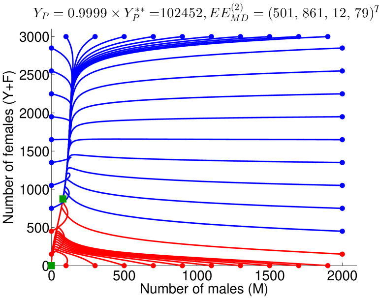
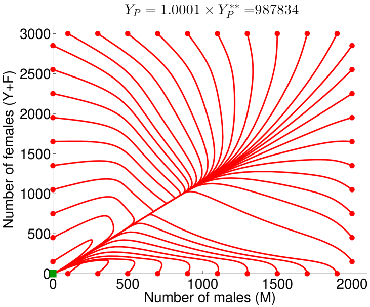
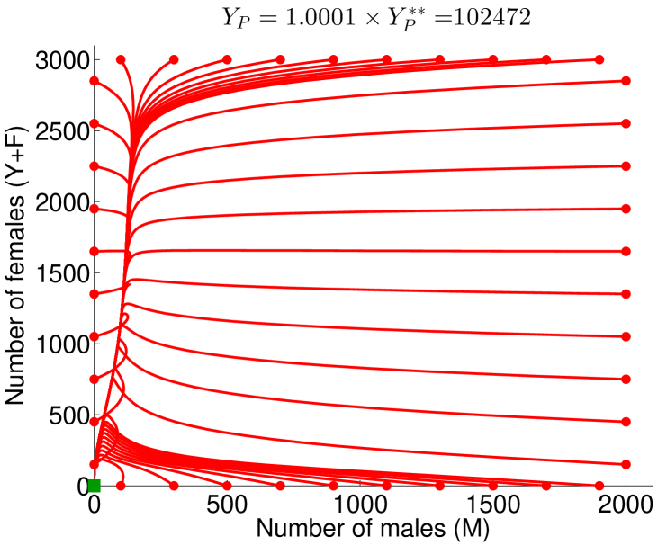
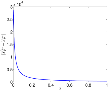
Mathematical model for pest-insect control using mating disruption and trapping

Roumen Anguelova, Claire Dufourda, Yves Dumontb,111 Corresponding author: yves.dumont@cirad.fr
aDepartment of Mathematics and Applied Mathematics, University of Pretoria,
Pretoria, South Africa
bCIRAD, Umr AMAP, Montpellier, France
Abstract

Controlling pest insects is a challenge of main importance to preserve crop production. In the context of Integrated Pest Management (IPM) programs, we develop a generic model to study the impact of mating disruption control using an artificial female pheromone to confuse males and adversely affect their mating opportunities. Consequently the reproduction rate is diminished leading to a decline in the population size. For more efficient control, trapping is used to capture the males attracted to the artificial pheromone. The model, derived from biological and ecological assumptions, is governed by a system of ODEs. A theoretical analysis of the model without control is first carried out to establish the properties of the endemic equilibrium. Then, control is added and the theoretical analysis of the model enables to identify threshold values of pheromone which are practically interesting for field applications. In particular, we show that there is a threshold above which the global asymptotic stability of the trivial equilibrium is ensured, i.e. the population goes to extinction. Finally we illustrate the theoretical results via numerical experiments.

key words:

Ordinary differential equations; monotone dymanical system; stability analysis; pest control; pheromone traps; mating disruption; insect trapping

1 Introduction

Pest insects are responsible for considerable damages on crops all over the world. Their presence can account for high production losses having repercussions on trading and exports as well on the sustainability of small farmers whose incomes entirely rely on their production. Exotic pests, can be particularly harmful as they can exhibit high invading potential due to the lack of natural enemies and their capacity to adapt to wide range of hosts and/or climate conditions. Therefore, pest management is essential to prevent devastating impact on economy, food security, social life, health and biodiversity.

Chemical pesticides have long been used to control pest populations. However, their extensive use can have undesired side effects on the surrounding environment, such as reduction of the pest’s natural enemies and pollution. Further, the development of insect resistance to the chemical lead to the need of using stronger and more toxic pesticides to maintain their efficacy. Thus, extensive use of pesticides is not a sustainable solution for pest control. Constant efforts are being made to reduce the toxicity of the pesticides for applicators and consumers, and alternative methods are being developed or improved to satisfy the charter of Integrated Pest Management (IPM) programs [5]. IPM aims to maintain pest population at low economic and epidemiological risk while respecting specific ecological and toxicological environmentally friendly requirements.

The Sterile Insect Technique (SIT), Mass Annihilation Technique (MAT) or mating disruption are examples of methods part of IPM strategies. SIT consists in releasing large numbers of sterilised males to compete with wild males for female insemination, reducing the number of viable offspring, while MAT consists in reducing the number of one or both sexes by trapping using a species-specific attractant. Pheromones or para-pheromones are often used to manipulate the behaviour of a specific species [36, 25]. In this work, particular interest is given to mating disruption control which aims to obstruct the communication among sexual partners using lures to reduce the mating rate of the pest and thus lead to long-term reduction of the population [14].

Mating disruption using pheromones has been widely studied to control moth pests [11, 15] on various types of crops. An early demonstration of the applicability of MAT has been shown for the eradication of Bactrocera doraslis in the Okinawa Islands in 1984 [29]. More recently, the method has shown to be successful for the control of Tuta absoluta on tomato crops in Italian greenhouses [16]. Other successful cases are reported in [15], such as for the control of the pink bollworm Pectinophora gossypiella which attacks cotton, or the apple codling moth Cydia pomonella. However, mating disruption has sometimes been a failure as for the control of the coffee leaf miner Leucoptera coffeela [1] or for the control of the tomato pest Tuta absoluta mentioned above in open field conditions [31] where mating disruption did not manage to reduce the pest population. According to [1, 31], the failure of the method may be attributed to composition and dosage of the pheromone and/or to a high abundance of insects. For mating disruption success, understanding the attraction mechanisms of the pest to the pheromone is important, like the minimum level response, the distance of attraction or the formulation of the pheromone used. Environmental constrains are also crucial factors to take into account. These include the climate, the wind, the crop’s foliage, etc. Further, the population size must be accounted for in order to design appropriate control strategies. Thus, planning efficient and cost effective control is a real challenge which can explain the failure of the experiments mentioned above. Mathematical modelling can be very helpful to get a better understanding on the dynamics of the pest population, and various control strategies can be studied to optimise the control. Here we combine mating disruption using female-sex pheromones lures to attract males away from females in order to reduce the mating opportunities adversely affecting the rate reproduction. For more efficient control, lures can be placed in traps to reduce the male population. In 1955, Knipling proposed a numerical model to assess the effect of the release of sterile males on an insect population where the rate of fertilisation depends on the density of fertile males available for mating [26]. It is worth mentioning that in terms of modelling significant similarities can be found between MAT control and SIT control as the purpose of both methods is to affect the capacity of reproduction of the species. In the seminal works of Knipling et al. [28, 27], several approaches for the suppression of insect populations among which MAT and SIT. Further, an overview on the mathematical models for SIT control which of relevance to mating disruption control can be found in [20, Chapter 2.5].

In this paper we built a generic model for the control of a pest population using mating disruption and trapping to study the effort required to reduce the population size below harmful level. The model is derived using general knowledge or assumptions on insects’ biology and ecology. We consider a compartmental approach based on the life cycle and mating behaviour to model the temporal dynamics of the population which is governed by a system of Ordinary Differential Equations (ODE). A theoretical analysis of the model is carried out to discuss the efficiency of the control using pheromone traps depending on the strength of the lure and the trapping efficacy. In particular we study the properties of the equilibria using the pheromone as a bifurcation parameter. We identify two threshold values of practical importance. One corresponds to the minimum amount of lure required to affect the female population equilibrium, while the second one is the threshold above which extinction of the population is achieved. We also show that on small enough populations, at invasion stage for instance, extinction may be achieved with a small amount of lure. We also show that combining mating disruption with trapping significantly reduces the amount of pheromone needed to obtain a full control of the population. The modelling approach for mating disruption control considered in [10, 8, 22] where MAT control is modelled via discrete density-dependent models. In the later, the authors identified a threshold value for the amount of pheromones above which the control of an insect population is possible. Similar qualitative results may be found in  [9] in the case of SIT control, however not presented as in such depth as in the present study.

In the first section, we give a description of the model without control and analyse it theoretically. In the following section we describe the model with control. To model the impact of the mating disruption, we use a similar approach as the one proposed by Barclay and Van den Driessche [10], where the amount of the artificial pheromone is given in terms of equivalent number of females. The model is studied theoretically, identifying threshold values which determine changes in the dynamics of the population. Finally, we perform numerical simulations to illustrate the theoretical results and we discuss their biological relevance.

2 The compartmental model for the dynamics of the insect

We consider a generic model to describe the dynamics of a pest insect population based on biological and behavioural assumptions. For many pest species, such as fruit flies or moths, two main development stages can be considered: the immature stage, denoted I𝐼I, which gathers eggs, larvae and pupae, and the adult stage. Typically, the adult female is the one responsible for causing direct damage to the host when laying her eggs. We split the adult females in two compartments, the females available for mating denoted Y𝑌Y, and the fertilised females denoted F𝐹F. We assume that a mating female needs to mate with a male in order to pass into the compartment of the fertilised females and be able to deposit her eggs. Therefore, we also add a male compartment, denoted M𝑀M, to study how the abundance of males impacts the transfer rate from Y𝑌Y to F𝐹F. We make the model sufficiently generic such that multiple mating can occur, which implies that fertilised females can become mating female again.

We denote r𝑟r the proportion of females emerging from the immature stage and entering the mating females compartment. Thus a proportion of (1r)1𝑟(1-r) on the immature enter the male compartment after emergence. We assume that the time needed for an egg laid to emergence is 1/νI1subscript𝜈𝐼1/\nu_{I}, thus the transfer rate from I𝐼I to Y𝑌Y or M𝑀M is νIsubscript𝜈𝐼\nu_{I}. Then, when males are in sufficient abundance to ensure the fertilisation of all the females available for mating, the transfer rate from Y𝑌Y to F𝐹F is νYsubscript𝜈𝑌\nu_{Y}. However, if males are scarce, and if γ𝛾\gamma is the number of females that can be fertilised by a single male, then only a proportion γMY𝛾𝑀𝑌\frac{\gamma M}{Y} of Y𝑌Y-females can pass into the F𝐹F-females compartment. Therefore, the transfer rate from Y𝑌Y to F𝐹F is modelled by the non-linear term νYmin{γMY,1}subscript𝜈𝑌𝛾𝑀𝑌1\nu_{Y}\min\{\frac{\gamma M}{Y},1\}. Moreover, fertilised females go back to the mating females compartment with a rate of δ𝛿\delta. Further, the fertilised females supply the immature compartment with a rate b(1IK)𝑏1𝐼𝐾b\left(1-\frac{I}{K}\right), where b𝑏b is the intrinsic egg laying rate, while K𝐾K is the carrying capacity of the hosts. Finally, parameters μIsubscript𝜇𝐼\mu_{I}, μYsubscript𝜇𝑌\mu_{Y}, μFsubscript𝜇𝐹\mu_{F} are respectively the death rates of compartments I𝐼I, Y𝑌Y, F𝐹F and M𝑀M. The flow diagram of the insects’ dynamics is represented in Figure 1.
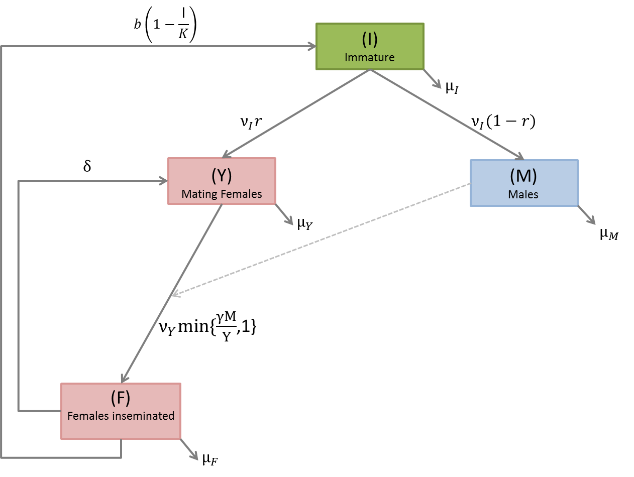
Refer to caption
Figure 1: Life cycle of the insect.

The model is governed by the following system of ODEs:

{dIdt=b(1IK)F(νI+μI)I,dYdt=rνIIνYmin{γMY,1}Y+δFμYY,dFdt=νYmin{γMY,1}YδFμFF,dMdt=(1r)νII(μM)M.cases𝑑𝐼𝑑𝑡𝑏1𝐼𝐾𝐹subscript𝜈𝐼subscript𝜇𝐼𝐼missing-subexpressionmissing-subexpressionmissing-subexpression𝑑𝑌𝑑𝑡𝑟subscript𝜈𝐼𝐼subscript𝜈𝑌𝛾𝑀𝑌1𝑌𝛿𝐹subscript𝜇𝑌𝑌missing-subexpressionmissing-subexpressionmissing-subexpression𝑑𝐹𝑑𝑡subscript𝜈𝑌𝛾𝑀𝑌1𝑌𝛿𝐹subscript𝜇𝐹𝐹missing-subexpressionmissing-subexpressionmissing-subexpression𝑑𝑀𝑑𝑡1𝑟subscript𝜈𝐼𝐼subscript𝜇𝑀𝑀\left\{\begin{array}[]{lcl}\frac{dI}{dt}&=&b\left(1-\frac{I}{K}\right)F-\left(\nu_{I}+\mu_{I}\right)I,\\ &&\\ \frac{dY}{dt}&=&r\nu_{I}I-\nu_{Y}\min\{\frac{\gamma M}{Y},1\}Y+\delta F-\mu_{Y}Y,\\ &&\\ \frac{dF}{dt}&=&\nu_{Y}\min\{\frac{\gamma M}{Y},1\}Y-\delta F-\mu_{F}F,\\ &&\\ \frac{dM}{dt}&=&(1-r)\nu_{I}I-(\mu_{M})M.\end{array}\right. (1)

The list of the parameters used in the model are summarized in Table 1. They are taken from [21] in order to perform numerical experiments.

Parameter Description Unit Value
b Intrinsic egg laying rate female-1day-1 9.2729.2729.272
r Female to male ratio - 0.570.570.57
K Carrying capacity - 100010001000
γ𝛾\gamma Females fertilised by a single male - 444
μIsubscript𝜇𝐼\mu_{I} Mortality rate in the I𝐼I compartment day-1 1/151151/15
μYsubscript𝜇𝑌\mu_{Y} Mortality rate in the Y𝑌Y compartment day-1 1/75.1175.11/75.1
μFsubscript𝜇𝐹\mu_{F} Mortality rate in the F𝐹F compartment day-1 1/75.1175.11/75.1
μMsubscript𝜇𝑀\mu_{M} Mortality rate in the M𝑀M compartment day-1 1/86.4186.41/86.4
νIsubscript𝜈𝐼\nu_{I} Transfer rate from I𝐼I to Y𝑌Y day-1 1/24.6124.61/24.6
νYsubscript𝜈𝑌\nu_{Y} Transfer rate from Y𝑌Y to F𝐹F day-1 0.50.50.5
δ𝛿\delta Transfer rate from F𝐹F to Y𝑌Y day-1 0.10.10.1
Table 1: List of parameters and there values used in the numerical simulations.

2.1 Theoretical analysis of the model

The theoretical analysis of the model is carried out for the case of male abundance and the case of male scarcity. These two cases are separated by the hyperplane Y=γM𝑌𝛾𝑀Y=\gamma M. The analysis of the two systems can be carried out independently on the orthant +4subscriptsuperscript4\mathbb{R}^{4}_{+}.

2.1.1 Case 1: Male abundance

In the case of male abundance, we recover the same model developed and studied in [19]. However, we follow another approach for the theoretical study. The system can be written in the vector form

dxdt=f(x),𝑑𝑥𝑑𝑡𝑓𝑥\frac{dx}{dt}=f(x), (2)

with x=(I,Y,F,M)T𝑥superscript𝐼𝑌𝐹𝑀𝑇x=(I,Y,F,M)^{T}, and

f(x)=(b(1IK)F(νI+μI)IrνII+δF(νY+μY)YνYY(δ+μF)F(1r)νIIμMM).𝑓𝑥𝑏1𝐼𝐾𝐹subscript𝜈𝐼subscript𝜇𝐼𝐼𝑟subscript𝜈𝐼𝐼𝛿𝐹subscript𝜈𝑌subscript𝜇𝑌𝑌subscript𝜈𝑌𝑌𝛿subscript𝜇𝐹𝐹1𝑟subscript𝜈𝐼𝐼subscript𝜇𝑀𝑀f(x)=\left(\begin{array}[]{c}b\left(1-\frac{I}{K}\right)F-(\nu_{I}+\mu_{I})I\\ r\nu_{I}I+\delta F-(\nu_{Y}+\mu_{Y})Y\\ \nu_{Y}Y-(\delta+\mu_{F})F\\ (1-r)\nu_{I}I-\mu_{M}M\end{array}\right). (3)

Note that the right hand side of system (2), f(x)𝑓𝑥f(x), is continuous and locally Lipschitz, so uniqueness and local existence of the solution are guaranteed. In proving the global properties we will use the fact that the system is cooperative on +4subscriptsuperscript4\mathbb{R}^{4}_{+}, that is the growth in any compartment impacts positively on the growth of all other compartments. For completeness of the exposition some basics of the theory of cooperative systems is given in Appendix C. Using Theorem 10, the system (2) is cooperative on ΩK={x+4:IK}subscriptΩ𝐾conditional-set𝑥subscriptsuperscript4𝐼𝐾\Omega_{K}=\{x\in\mathbb{R}^{4}_{+}:I\leq K\} because the non-diagonal entries of the Jacobian matrix of f𝑓f

𝒥f=((νI+μI+bFK)0b(1IK)0rνI(νY+μY)δ00νY(μF+δ)0(1r)νI00μM),subscript𝒥𝑓subscript𝜈𝐼subscript𝜇𝐼𝑏𝐹𝐾0𝑏1𝐼𝐾0𝑟subscript𝜈𝐼subscript𝜈𝑌subscript𝜇𝑌𝛿00subscript𝜈𝑌subscript𝜇𝐹𝛿01𝑟subscript𝜈𝐼00subscript𝜇𝑀\mathcal{J}_{f}=\left(\begin{array}[]{cccc}-\left(\nu_{I}+\mu_{I}+b\frac{F}{K}\right)&0&b(1-\frac{I}{K})&0\\ r\nu_{I}&-(\nu_{Y}+\mu_{Y})&\delta&0\\ 0&\nu_{Y}&-(\mu_{F}+\delta)&0\\ (1-r)\nu_{I}&0&0&-\mu_{M}\\ \end{array}\right), (4)

are non-negative on ΩKsubscriptΩ𝐾\Omega_{K}.

The persistence of a population is typically linked to its Basic Offspring Number. For simple population models the basic offspring number is defined as the number of offspring produced by a single individual in their life time provided abundant resource is available. In general, the definition could be more complicated and its value is computed by using the next generation method. For the model in (2) the Basic Offspring Number is

𝒩0=brνIνY(μI+νI)((νY+μY)(δ+μF)δνY).subscript𝒩0𝑏𝑟subscript𝜈𝐼subscript𝜈𝑌subscript𝜇𝐼subscript𝜈𝐼subscript𝜈𝑌subscript𝜇𝑌𝛿subscript𝜇𝐹𝛿subscript𝜈𝑌\mathcal{N}_{0}=\frac{br\nu_{I}\nu_{Y}}{(\mu_{I}+\nu_{I})((\nu_{Y}+\mu_{Y})(\delta+\mu_{F})-\delta\nu_{Y})}. (5)

In this paper we will use 𝒩0subscript𝒩0\mathcal{N}_{0} only as a threshold parameter. The persistence when 𝒩0>1subscript𝒩01\mathcal{N}_{0}>1 and the extinction when 𝒩0<1subscript𝒩01\mathcal{N}_{0}<1 are given direct proofs. Hence, we will not discuss the details on specific properties of the number. For completeness of the exposition the computation of (5) is given in Appendix A.

Theorem 1.
  • a)

    The system of ODE (2) defines a positive dynamical system on +4subscriptsuperscript4\mathbb{R}^{4}_{+}.

  • b)

    If 𝒩01subscript𝒩01\mathcal{N}_{0}\leq 1 then TE=(0,0,0,0)T𝑇𝐸superscript0000𝑇TE=(0,0,0,0)^{T} is a globally asymptotically stable (GAS) equilibrium.

  • c)

    If 𝒩0>1subscript𝒩01\mathcal{N}_{0}>1 then TE𝑇𝐸TE is an unstable equilibrium and the system admits a positive equilibrium EE=(I,Y,F,M)T𝐸superscript𝐸superscriptsuperscript𝐼superscript𝑌superscript𝐹superscript𝑀𝑇EE^{*}=(I^{*},Y^{*},F^{*},M^{*})^{T}, where

    Isuperscript𝐼\displaystyle I^{*} =\displaystyle= (11𝒩0)K,11subscript𝒩0𝐾\displaystyle\left(1-\frac{1}{\mathcal{N}_{0}}\right)K,
    Ysuperscript𝑌\displaystyle Y^{*} =\displaystyle= rνI(δ+μF)(νY+μY)(δ+μF)δνY(11𝒩0)K,𝑟subscript𝜈𝐼𝛿subscript𝜇𝐹subscript𝜈𝑌subscript𝜇𝑌𝛿subscript𝜇𝐹𝛿subscript𝜈𝑌11subscript𝒩0𝐾\displaystyle\frac{r\nu_{I}(\delta+\mu_{F})}{(\nu_{Y}+\mu_{Y})(\delta+\mu_{F})-\delta\nu_{Y}}\left(1-\frac{1}{\mathcal{N}_{0}}\right)K,
    Fsuperscript𝐹\displaystyle F^{*} =\displaystyle= rνIνY(νY+μY)(δ+μF)δνY(11𝒩0)K,𝑟subscript𝜈𝐼subscript𝜈𝑌subscript𝜈𝑌subscript𝜇𝑌𝛿subscript𝜇𝐹𝛿subscript𝜈𝑌11subscript𝒩0𝐾\displaystyle\frac{r\nu_{I}\nu_{Y}}{(\nu_{Y}+\mu_{Y})(\delta+\mu_{F})-\delta\nu_{Y}}\left(1-\frac{1}{\mathcal{N}_{0}}\right)K,
    Msuperscript𝑀\displaystyle M^{*} =\displaystyle= (1r)νIμM(11𝒩0)K,1𝑟subscript𝜈𝐼subscript𝜇𝑀11subscript𝒩0𝐾\displaystyle\frac{(1-r)\nu_{I}}{\mu_{M}}\left(1-\frac{1}{\mathcal{N}_{0}}\right)K,

    which is a globally asymptotically stable (GAS) on +4{x+4:I=Y=F=0}subscriptsuperscript4conditional-set𝑥subscriptsuperscript4𝐼𝑌𝐹0\mathbb{R}^{4}_{+}\setminus\{x\in\mathbb{R}^{4}_{+}:I=Y=F=0\}.

Proof.

a) Let q𝑞q\in\mathbb{R}, qK𝑞𝐾q\geq K. Denote

yq=(KrνI(δ+μF)(νY+μY)(δ+μF)δνYqrνIνY(νY+μY)(δ+μF)δνYq(1r)νIμMq)subscript𝑦𝑞𝐾𝑟subscript𝜈𝐼𝛿subscript𝜇𝐹subscript𝜈𝑌subscript𝜇𝑌𝛿subscript𝜇𝐹𝛿subscript𝜈𝑌𝑞𝑟subscript𝜈𝐼subscript𝜈𝑌subscript𝜈𝑌subscript𝜇𝑌𝛿subscript𝜇𝐹𝛿subscript𝜈𝑌𝑞1𝑟subscript𝜈𝐼subscript𝜇𝑀𝑞y_{q}=\left(\begin{array}[]{c}K\\ \frac{r\nu_{I}(\delta+\mu_{F})}{(\nu_{Y}+\mu_{Y})(\delta+\mu_{F})-\delta\nu_{Y}}q\\ \frac{r\nu_{I}\nu_{Y}}{(\nu_{Y}+\mu_{Y})(\delta+\mu_{F})-\delta\nu_{Y}}q\\ \frac{(1-r)\nu_{I}}{\mu_{M}}q\\ \end{array}\right) (6)

We have f(0)=0𝑓00f(\textbf{0})=\textbf{0} and f(yq)0𝑓subscript𝑦𝑞0f(y_{q})\leq\textbf{0}. Then, from Theorem 13 it follows that (2) defines a positive dynamical system on [0,yq]0subscript𝑦𝑞[\textbf{0},y_{q}]. That is x[0,yq]for-all𝑥0subscript𝑦𝑞\forall x\in[\textbf{0},y_{q}], the problem (2), given an initial condition x(0)=x0[0,yq]𝑥0subscript𝑥00subscript𝑦𝑞x(0)=x_{0}\in[\textbf{0},y_{q}], admits a unique solution for all t[0,]𝑡0t\in[0,\infty] in [0,yq]0subscript𝑦𝑞[\textbf{0},y_{q}] [4]. Hence (2) defines a positive dynamical system on ΩK=qK[0,yq]subscriptΩ𝐾subscript𝑞𝐾0subscript𝑦𝑞\Omega_{K}=\cup_{q\geq K}[\textbf{0},y_{q}]. Let now x0+4ΩKsubscript𝑥0subscriptsuperscript4subscriptΩ𝐾x_{0}\in\mathbb{R}^{4}_{+}\setminus\Omega_{K}. Using that the vector field defined by f𝑓f points inwards on the boundary of +4subscriptsuperscript4\mathbb{R}^{4}_{+} we deduce that the solution initiated at x0subscript𝑥0x_{0} remains in +4subscriptsuperscript4\mathbb{R}^{4}_{+}. Then one can see from the first equation of (2) that I(t)𝐼𝑡I(t) decreases until the solution is absorbed in ΩKsubscriptΩ𝐾\Omega_{K}. Then (2) defines a dynamical system on +4subscriptsuperscript4\mathbb{R}^{4}_{+} with ΩKsubscriptΩ𝐾\Omega_{K} being an absorbing set.

b)Solving f(x)=0𝑓𝑥0f(x)=0 yields two solutions TE𝑇𝐸TE and EE𝐸superscript𝐸EE^{*}. When 𝒩01subscript𝒩01\mathcal{N}_{0}\leq 1 TE𝑇𝐸TE is the only equilibrium in +4subscriptsuperscript4\mathbb{R}^{4}_{+}. Then for any qK𝑞𝐾q\geq K TE𝑇𝐸TE is the only equilibrium in [0,yq]0subscript𝑦𝑞[\textbf{0},y_{q}]. It follows from Theorem 13 that it is GAS on [0,yq]0subscript𝑦𝑞[\textbf{0},y_{q}]. Therefore, TE𝑇𝐸TE is GAS on ΩKsubscriptΩ𝐾\Omega_{K} and further on +4superscriptsubscript4\mathbb{R}_{+}^{4} by using that ΩKsubscriptΩ𝐾\Omega_{K} is an absorption set.

c) For ε(0,I)𝜀0superscript𝐼\varepsilon\in(0,I^{*}) we consider the vector

zε=(εrνI(δ+μF)(νY+μY)(δ+μF)δνYεrνIνY(νY+μY)(δ+μF)δνYε(1r)νIμMε).subscript𝑧𝜀𝜀𝑟subscript𝜈𝐼𝛿subscript𝜇𝐹subscript𝜈𝑌subscript𝜇𝑌𝛿subscript𝜇𝐹𝛿subscript𝜈𝑌𝜀𝑟subscript𝜈𝐼subscript𝜈𝑌subscript𝜈𝑌subscript𝜇𝑌𝛿subscript𝜇𝐹𝛿subscript𝜈𝑌𝜀1𝑟subscript𝜈𝐼subscript𝜇𝑀𝜀z_{\varepsilon}=\left(\begin{array}[]{c}\varepsilon\\ \frac{r\nu_{I}(\delta+\mu_{F})}{(\nu_{Y}+\mu_{Y})(\delta+\mu_{F})-\delta\nu_{Y}}\varepsilon\\ \frac{r\nu_{I}\nu_{Y}}{(\nu_{Y}+\mu_{Y})(\delta+\mu_{F})-\delta\nu_{Y}}\varepsilon\\ \frac{(1-r)\nu_{I}}{\mu_{M}}\varepsilon\\ \end{array}\right). (7)

Straightforward computations show that dYdt(zε)=dFdt(zε)=dMdt(zε)=0𝑑𝑌𝑑𝑡subscript𝑧𝜀𝑑𝐹𝑑𝑡subscript𝑧𝜀𝑑𝑀𝑑𝑡subscript𝑧𝜀0\frac{dY}{dt}(z_{\varepsilon})=\frac{dF}{dt}(z_{\varepsilon})=\frac{dM}{dt}(z_{\varepsilon})=0, and that we have

dIdt(zε)=b(1εK)rνIνY(νY+μY)(δ+μF)δνYε(νI+μI)ε,=brνIνY(νY+μY)(δ+μF)δνYεbrνIνY(νY+μY)(δ+μF)δνYε2K(νI+μI)ε=(νI+μI)𝒩0ε(νI+μI)𝒩0ε2K(νI+μI)ε=(νI+μI)(𝒩0(1εK)1)ε=(νI+μI)𝒩0K(Iε)ε>0.𝑑𝐼𝑑𝑡subscript𝑧𝜀𝑏1𝜀𝐾𝑟subscript𝜈𝐼subscript𝜈𝑌subscript𝜈𝑌subscript𝜇𝑌𝛿subscript𝜇𝐹𝛿subscript𝜈𝑌𝜀subscript𝜈𝐼subscript𝜇𝐼𝜀missing-subexpression𝑏𝑟subscript𝜈𝐼subscript𝜈𝑌subscript𝜈𝑌subscript𝜇𝑌𝛿subscript𝜇𝐹𝛿subscript𝜈𝑌𝜀𝑏𝑟subscript𝜈𝐼subscript𝜈𝑌subscript𝜈𝑌subscript𝜇𝑌𝛿subscript𝜇𝐹𝛿subscript𝜈𝑌superscript𝜀2𝐾subscript𝜈𝐼subscript𝜇𝐼𝜀missing-subexpressionsubscript𝜈𝐼subscript𝜇𝐼subscript𝒩0𝜀subscript𝜈𝐼subscript𝜇𝐼subscript𝒩0superscript𝜀2𝐾subscript𝜈𝐼subscript𝜇𝐼𝜀missing-subexpressionsubscript𝜈𝐼subscript𝜇𝐼subscript𝒩01𝜀𝐾1𝜀missing-subexpressionsubscript𝜈𝐼subscript𝜇𝐼subscript𝒩0𝐾superscript𝐼𝜀𝜀0\begin{array}[]{lcl}\frac{dI}{dt}(z_{\varepsilon})&=&b\left(1-\frac{\varepsilon}{K}\right)\frac{r\nu_{I}\nu_{Y}}{(\nu_{Y}+\mu_{Y})(\delta+\mu_{F})-\delta\nu_{Y}}\varepsilon-\left(\nu_{I}+\mu_{I}\right)\varepsilon,\\ &=&\frac{br\nu_{I}\nu_{Y}}{(\nu_{Y}+\mu_{Y})(\delta+\mu_{F})-\delta\nu_{Y}}\varepsilon-\frac{br\nu_{I}\nu_{Y}}{(\nu_{Y}+\mu_{Y})(\delta+\mu_{F})-\delta\nu_{Y}}\frac{\varepsilon^{2}}{K}-\left(\nu_{I}+\mu_{I}\right)\varepsilon\\ &=&(\nu_{I}+\mu_{I})\mathcal{N}_{0}\varepsilon-(\nu_{I}+\mu_{I})\mathcal{N}_{0}\frac{\varepsilon^{2}}{K}-\left(\nu_{I}+\mu_{I}\right)\varepsilon\\ &=&(\nu_{I}+\mu_{I})\left(\mathcal{N}_{0}(1-\frac{\varepsilon}{K})-1\right)\varepsilon\\ &=&(\nu_{I}+\mu_{I})\frac{\mathcal{N}_{0}}{K}(I^{*}-\varepsilon)\varepsilon>0.\end{array}

Thus, f(xε)0𝑓subscript𝑥𝜀0f(x_{\varepsilon})\geq\textbf{0}. For any ε(0,I)𝜀0superscript𝐼\varepsilon\in(0,I^{*}) and q(ε,K]𝑞𝜀𝐾q\in(\varepsilon,K] EE𝐸superscript𝐸EE^{*} is a unique equilibrium in the interval [zε,yq]subscript𝑧𝜀subscript𝑦𝑞[z_{\varepsilon},y_{q}] and hence, by Theorem 13, it is GAS on this interval. Therefore, EE𝐸superscript𝐸EE^{*} is GAS also on interior(ΩK)𝑖𝑛𝑡𝑒𝑟𝑖𝑜𝑟subscriptΩ𝐾interior(\Omega_{K}). Using further that (i) if either I(0)𝐼0I(0) or Y(0)𝑌0Y(0) or F(0)𝐹0F(0) is positive then x(t)>0𝑥𝑡0x(t)>0 for all t>0𝑡0t>0 and that (ii) ΩKsubscriptΩ𝐾\Omega_{K} is an absorbing set, we obtain that EE𝐸superscript𝐸EE^{*} attracts all solution in +4subscriptsuperscript4\mathbb{R}^{4}_{+} except the ones initiated on the M𝑀M-axis. ∎

2.1.2 Case 2: Male scarcity

Next we consider the case when males are scarce, that is when γM<Y𝛾𝑀𝑌\gamma M<Y. The system assumes the form

{dIdt=b(1IK)F(νI+μI)I,dYdt=rνIIνYγM+δFμYY,dFdt=νYγM(δ+μF)F,dMdt=(1r)νIIμMM.cases𝑑𝐼𝑑𝑡𝑏1𝐼𝐾𝐹subscript𝜈𝐼subscript𝜇𝐼𝐼missing-subexpressionmissing-subexpressionmissing-subexpression𝑑𝑌𝑑𝑡𝑟subscript𝜈𝐼𝐼subscript𝜈𝑌𝛾𝑀𝛿𝐹subscript𝜇𝑌𝑌missing-subexpressionmissing-subexpressionmissing-subexpression𝑑𝐹𝑑𝑡subscript𝜈𝑌𝛾𝑀𝛿subscript𝜇𝐹𝐹missing-subexpressionmissing-subexpressionmissing-subexpression𝑑𝑀𝑑𝑡1𝑟subscript𝜈𝐼𝐼subscript𝜇𝑀𝑀\left\{\begin{array}[]{lcl}\frac{dI}{dt}&=&b\left(1-\frac{I}{K}\right)F-\left(\nu_{I}+\mu_{I}\right)I,\\ &&\\ \frac{dY}{dt}&=&r\nu_{I}I-\nu_{Y}\gamma M+\delta F-\mu_{Y}Y,\\ &&\\ \frac{dF}{dt}&=&\nu_{Y}\gamma M-(\delta+\mu_{F})F,\\ &&\\ \frac{dM}{dt}&=&(1-r)\nu_{I}I-\mu_{M}M.\end{array}\right. (8)

It is easy to see that the second equation can be decoupled. The system of the remaining 333 equations is of the form

dudt=g(u),𝑑𝑢𝑑𝑡𝑔𝑢\frac{du}{dt}=g(u), (9)

where u=(IFM)𝑢𝐼𝐹𝑀u=\left(\begin{array}[]{c}I\\ F\\ M\\ \end{array}\right) and g(u)=(b(1IK)F(νI+μI)IνYγM(δ+μF)F(1r)νIIμMM)𝑔𝑢𝑏1𝐼𝐾𝐹subscript𝜈𝐼subscript𝜇𝐼𝐼subscript𝜈𝑌𝛾𝑀𝛿subscript𝜇𝐹𝐹1𝑟subscript𝜈𝐼𝐼subscript𝜇𝑀𝑀g(u)=\left(\begin{array}[]{c}b\left(1-\frac{I}{K}\right)F-\left(\nu_{I}+\mu_{I}\right)I\\ \nu_{Y}\gamma M-(\delta+\mu_{F})F\\ (1-r)\nu_{I}I-\mu_{M}M\\ \end{array}\right). The non-diagonal entries of the Jacobian of g𝑔g,

𝒥g=((νI+μI+bFK)b(1IK)00(δ+μF)νYγ(1r)νI0μM),subscript𝒥𝑔subscript𝜈𝐼subscript𝜇𝐼𝑏𝐹𝐾𝑏1𝐼𝐾00𝛿subscript𝜇𝐹subscript𝜈𝑌𝛾1𝑟subscript𝜈𝐼0subscript𝜇𝑀\mathcal{J}_{g}=\left(\begin{array}[]{ccc}-(\nu_{I}+\mu_{I}+b\frac{F}{K})&b\left(1-\frac{I}{K}\right)&0\\ 0&-(\delta+\mu_{F})&\nu_{Y}\gamma\\ (1-r)\nu_{I}&0&-\mu_{M}\\ \end{array}\right),

are non-negative. Hence the system (9) is cooperative. The Basic Offspring Number for system (9) is

𝒩^0=bγ(1r)νIνY(νI+μI)(δ+μF)μM.subscript^𝒩0𝑏𝛾1𝑟subscript𝜈𝐼subscript𝜈𝑌subscript𝜈𝐼subscript𝜇𝐼𝛿subscript𝜇𝐹subscript𝜇𝑀\hat{\mathcal{N}}_{0}=\frac{b\gamma(1-r)\nu_{I}\nu_{Y}}{(\nu_{I}+\mu_{I})(\delta+\mu_{F})\mu_{M}}. (10)

The following theorem describes the properties of system (9).

Theorem 2.
  • a)

    The system of ODE (9) defines a positive dynamical system on +3subscriptsuperscript3\mathbb{R}^{3}_{+}.

  • b)

    If 𝒩^01subscript^𝒩01\hat{\mathcal{N}}_{0}\leq 1 then TE=(0,0,0)T𝑇𝐸superscript000𝑇TE=(0,0,0)^{T} is a globally asymptotically stable (GAS) equilibrium.

  • c)

    If 𝒩^0>1subscript^𝒩01\hat{\mathcal{N}}_{0}>1 then TE𝑇𝐸TE is an unstable equilibrium and the system admits a positive equilibrium EE^=(I^,F^,M^)^𝐸𝐸^𝐼^𝐹^𝑀\hat{EE}=(\hat{I},\hat{F},\hat{M}), where

    I^^𝐼\displaystyle\hat{I} =\displaystyle= (11𝒩^0)K,11subscript^𝒩0𝐾\displaystyle\left(1-\frac{1}{\hat{\mathcal{N}}_{0}}\right)K,
    F^^𝐹\displaystyle\hat{F} =\displaystyle= γ(1r)νIνY(δ+μF)μM(11𝒩^0)K,𝛾1𝑟subscript𝜈𝐼subscript𝜈𝑌𝛿subscript𝜇𝐹subscript𝜇𝑀11subscript^𝒩0𝐾\displaystyle\frac{\gamma(1-r)\nu_{I}\nu_{Y}}{(\delta+\mu_{F})\mu_{M}}\left(1-\frac{1}{\hat{\mathcal{N}}_{0}}\right)K,
    M^^𝑀\displaystyle\hat{M} =\displaystyle= (1r)νIμM(11𝒩^0)K,1𝑟subscript𝜈𝐼subscript𝜇𝑀11subscript^𝒩0𝐾\displaystyle\frac{(1-r)\nu_{I}}{\mu_{M}}\left(1-\frac{1}{\hat{\mathcal{N}}_{0}}\right)K,

    which is a globally asymptotically stable (GAS) on +3{x+3:I=F=0}subscriptsuperscript3conditional-set𝑥subscriptsuperscript3𝐼𝐹0\mathbb{R}^{3}_{+}\setminus\{x\in\mathbb{R}^{3}_{+}:I=F=0\}.

Proof.

a) Let q𝑞q\in\mathbb{R}, qK𝑞𝐾q\geq K. Denote

y^q=(Kγ(1r)νIνY(δ+μF)μMq(1r)νIμMq)subscript^𝑦𝑞𝐾𝛾1𝑟subscript𝜈𝐼subscript𝜈𝑌𝛿subscript𝜇𝐹subscript𝜇𝑀𝑞1𝑟subscript𝜈𝐼subscript𝜇𝑀𝑞\hat{y}_{q}=\left(\begin{array}[]{c}K\\ \frac{\gamma(1-r)\nu_{I}\nu_{Y}}{(\delta+\mu_{F})\mu_{M}}q\\ \frac{(1-r)\nu_{I}}{\mu_{M}}q\\ \end{array}\right) (11)

We have g(0)=0𝑔00g(\textbf{0})=\textbf{0} and g(y^q)0𝑔subscript^𝑦𝑞0g(\hat{y}_{q})\leq\textbf{0}. Then, from Theorem 13 it follows that (9) defines a positive dynamical system on [0,y^q]0subscript^𝑦𝑞[\textbf{0},\hat{y}_{q}]. Hence it defines a positive dynamical system on Ω^K=qK[0,y^q]subscript^Ω𝐾subscript𝑞𝐾0subscript^𝑦𝑞\hat{\Omega}_{K}=\cup_{q\geq K}[\textbf{0},\hat{y}_{q}]. Let now x0+3Ω^Ksubscript𝑥0subscriptsuperscript3subscript^Ω𝐾x_{0}\in\mathbb{R}^{3}_{+}\setminus\hat{\Omega}_{K}. Using that the vector field defined by g𝑔g points inwards on the boundary of +3subscriptsuperscript3\mathbb{R}^{3}_{+} we deduce that the solution initiated at x0subscript𝑥0x_{0} remains in +3subscriptsuperscript3\mathbb{R}^{3}_{+}. Then one can see from the first equation of (9) that I(t)𝐼𝑡I(t) decreases until the solution is absorbed in Ω^Ksubscript^Ω𝐾\hat{\Omega}_{K}. Then (9) defines a dynamical system on +3subscriptsuperscript3\mathbb{R}^{3}_{+} with Ω^Ksubscript^Ω𝐾\hat{\Omega}_{K} being an absorbing set.

b)Solving g(x)=0𝑔𝑥0g(x)=0 yields two solutions TE𝑇𝐸TE and EE^^𝐸𝐸\hat{EE}. When 𝒩^01subscript^𝒩01\hat{\mathcal{N}}_{0}\leq 1, TE𝑇𝐸TE is the only equilibrium in +3subscriptsuperscript3\mathbb{R}^{3}_{+}. Then for any qK𝑞𝐾q\geq K TE𝑇𝐸TE is the only equilibrium in [0,y^q]0subscript^𝑦𝑞[\textbf{0},\hat{y}_{q}]. It follows from Theorem 13 that it is GAS on [0,y^q]0subscript^𝑦𝑞[\textbf{0},\hat{y}_{q}]. Therefore, TE𝑇𝐸TE is GAS on Ω^Ksubscript^Ω𝐾\hat{\Omega}_{K} and further on +3superscriptsubscript3\mathbb{R}_{+}^{3} by using that Ω^Ksubscript^Ω𝐾\hat{\Omega}_{K} is an absorbing set.

c) For ε(0,I^)𝜀0^𝐼\varepsilon\in(0,\hat{I}) we consider the vector

z^ε=(εγ(1r)νIνY(δ+μF)μMε(1r)νIμMε).subscript^𝑧𝜀𝜀𝛾1𝑟subscript𝜈𝐼subscript𝜈𝑌𝛿subscript𝜇𝐹subscript𝜇𝑀𝜀1𝑟subscript𝜈𝐼subscript𝜇𝑀𝜀\hat{z}_{\varepsilon}=\left(\begin{array}[]{c}\varepsilon\\ \frac{\gamma(1-r)\nu_{I}\nu_{Y}}{(\delta+\mu_{F})\mu_{M}}\varepsilon\\ \frac{(1-r)\nu_{I}}{\mu_{M}}\varepsilon\\ \end{array}\right). (12)

Straightforward computations show that dFdt(z^ε)=dMdt(z^ε)=0𝑑𝐹𝑑𝑡subscript^𝑧𝜀𝑑𝑀𝑑𝑡subscript^𝑧𝜀0\frac{dF}{dt}(\hat{z}_{\varepsilon})=\frac{dM}{dt}(\hat{z}_{\varepsilon})=0, and that we have

dIdt(z^ε)=b(1εK)γ(1r)νIνY(δ+μF)μMε(νI+μI)ε=bγ(1r)νIνY(δ+μF)μMεbγ(1r)νIνY(δ+μF)μMε2K(νI+μI)ε=(νI+μI)𝒩^0ε(νI+μI)𝒩^0ε2K(νI+μI)ε=(νI+μI)(𝒩^0(1εK)1)ε=(νI+μI)𝒩^0K(I^ε)ε>0.𝑑𝐼𝑑𝑡subscript^𝑧𝜀𝑏1𝜀𝐾𝛾1𝑟subscript𝜈𝐼subscript𝜈𝑌𝛿subscript𝜇𝐹subscript𝜇𝑀𝜀subscript𝜈𝐼subscript𝜇𝐼𝜀missing-subexpression𝑏𝛾1𝑟subscript𝜈𝐼subscript𝜈𝑌𝛿subscript𝜇𝐹subscript𝜇𝑀𝜀𝑏𝛾1𝑟subscript𝜈𝐼subscript𝜈𝑌𝛿subscript𝜇𝐹subscript𝜇𝑀superscript𝜀2𝐾subscript𝜈𝐼subscript𝜇𝐼𝜀missing-subexpressionsubscript𝜈𝐼subscript𝜇𝐼subscript^𝒩0𝜀subscript𝜈𝐼subscript𝜇𝐼subscript^𝒩0superscript𝜀2𝐾subscript𝜈𝐼subscript𝜇𝐼𝜀missing-subexpressionsubscript𝜈𝐼subscript𝜇𝐼subscript^𝒩01𝜀𝐾1𝜀missing-subexpressionsubscript𝜈𝐼subscript𝜇𝐼subscript^𝒩0𝐾^𝐼𝜀𝜀0\begin{array}[]{lcl}\frac{dI}{dt}(\hat{z}_{\varepsilon})&=&b\left(1-\frac{\varepsilon}{K}\right)\frac{\gamma(1-r)\nu_{I}\nu_{Y}}{(\delta+\mu_{F})\mu_{M}}\varepsilon-\left(\nu_{I}+\mu_{I}\right)\varepsilon\\ &=&\frac{b\gamma(1-r)\nu_{I}\nu_{Y}}{(\delta+\mu_{F})\mu_{M}}\varepsilon-\frac{b\gamma(1-r)\nu_{I}\nu_{Y}}{(\delta+\mu_{F})\mu_{M}}\frac{\varepsilon^{2}}{K}-\left(\nu_{I}+\mu_{I}\right)\varepsilon\\ &=&(\nu_{I}+\mu_{I})\hat{\mathcal{N}}_{0}\varepsilon-(\nu_{I}+\mu_{I})\hat{\mathcal{N}}_{0}\frac{\varepsilon^{2}}{K}-\left(\nu_{I}+\mu_{I}\right)\varepsilon\\ &=&(\nu_{I}+\mu_{I})\left(\hat{\mathcal{N}}_{0}(1-\frac{\varepsilon}{K})-1\right)\varepsilon\\ &=&(\nu_{I}+\mu_{I})\frac{\hat{\mathcal{N}}_{0}}{K}(\hat{I}-\varepsilon)\varepsilon>0.\end{array}

Thus, g(xε)0𝑔subscript𝑥𝜀0g(x_{\varepsilon})\geq\textbf{0}. For any ε(0,I^)𝜀0^𝐼\varepsilon\in(0,\hat{I}) and q(ε,K]𝑞𝜀𝐾q\in(\varepsilon,K] EE^^𝐸𝐸\hat{EE} is a unique equilibrium in the interval [zε,yq]subscript𝑧𝜀subscript𝑦𝑞[z_{\varepsilon},y_{q}] and hence, by Theorem 13, it is GAS on this interval. Therefore, EE^^𝐸𝐸\hat{EE} is GAS also on interior(Ω^K)𝑖𝑛𝑡𝑒𝑟𝑖𝑜𝑟subscript^Ω𝐾interior(\hat{\Omega}_{K}). Using further that (i) if either I(0)𝐼0I(0) or F(0)𝐹0F(0) is positive then x(t)>0𝑥𝑡0x(t)>0 for all t>0𝑡0t>0 and that (ii) Ω^Ksubscript^Ω𝐾\hat{\Omega}_{K} is an absorbing set, we obtain that EE^^𝐸𝐸\hat{EE} attracts all solution in +3subscriptsuperscript3\mathbb{R}^{3}_{+} except the ones initiated on the M𝑀M-axis. ∎

It can be deduced from Theorem 2 that the non-trivial equilibrium value of Y𝑌Y is

Y^=rνI(δ+μF)μMνYγ(1r)νIμFμY(δ+μF)μM(11𝒩^0)K.^𝑌𝑟subscript𝜈𝐼𝛿subscript𝜇𝐹subscript𝜇𝑀subscript𝜈𝑌𝛾1𝑟subscript𝜈𝐼subscript𝜇𝐹subscript𝜇𝑌𝛿subscript𝜇𝐹subscript𝜇𝑀11subscript^𝒩0𝐾\hat{Y}=\frac{r\nu_{I}(\delta+\mu_{F})\mu_{M}-\nu_{Y}\gamma(1-r)\nu_{I}\mu_{F}}{\mu_{Y}(\delta+\mu_{F})\mu_{M}}\left(1-\frac{1}{\hat{\mathcal{N}}_{0}}\right)K. (13)

We note that the value of Y^^𝑌\hat{Y} and in general the value of the variable Y𝑌Y can be negative. Hence, the system of ODE (8) defines a dynamical system on +××+2subscriptsubscriptsuperscript2\mathbb{R}_{+}\times\mathbb{R}\times\mathbb{R}^{2}_{+}.

2.1.3 Conclusions for model (1)

In what follows we assume that the population has an endemic equilibrium. Otherwise, no control would be necessary. Further, it is natural to assume that, at equilibrium, there is abundance of males. In terms of the parameters of the model these assumptions can be written as:

1.1\displaystyle 1. 𝒩0>1,subscript𝒩01\displaystyle\mathcal{N}_{0}>1, (14)
2.2\displaystyle 2. Y<γM.superscript𝑌𝛾superscript𝑀\displaystyle Y^{*}<\gamma M^{*}. (15)

Under the assumptions (14) and (15) we have that EE^>0^𝐸𝐸0\hat{EE}>0 and Y^<γM^^𝑌𝛾^𝑀\hat{Y}<\gamma\hat{M}. Indeed, when 𝒩0>1subscript𝒩01\mathcal{N}_{0}>1, the inequality

𝒩^0𝒩0>1subscript^𝒩0subscript𝒩01\frac{\hat{\mathcal{N}}_{0}}{\mathcal{N}_{0}}>1

is equivalent to

γ>r(δ+μF)μM(1r)((νY+μY)(δ+μF)δνY),𝛾𝑟𝛿subscript𝜇𝐹subscript𝜇𝑀1𝑟subscript𝜈𝑌subscript𝜇𝑌𝛿subscript𝜇𝐹𝛿subscript𝜈𝑌\gamma>\frac{r(\delta+\mu_{F})\mu_{M}}{(1-r)((\nu_{Y}+\mu_{Y})(\delta+\mu_{F})-\delta\nu_{Y})},

which is ensured by (15). Therefore under assumptions (14) and (15) we have that 𝒩^0>1subscript^𝒩01\hat{\mathcal{N}}_{0}>1, and by Theorem 2, we have that the system (8) has a non-trivial equilibrium, which is globally asymptotically stable on +××+2{(I,Y,F,M)T:I=F=0}subscriptsubscriptsuperscript2conditional-setsuperscript𝐼𝑌𝐹𝑀𝑇𝐼𝐹0\mathbb{R}_{+}\times\mathbb{R}\times\mathbb{R}^{2}_{+}\setminus\{(I,Y,F,M)^{T}:I=F=0\}.

Further, under (15), we have

Y^γM^^𝑌𝛾^𝑀\displaystyle\hat{Y}-\gamma\hat{M} =\displaystyle= I^(rνI(δ+μF)μMνYγ(1r)νIμFμY(δ+μF)μMγ(1r)νIμM)^𝐼𝑟subscript𝜈𝐼𝛿subscript𝜇𝐹subscript𝜇𝑀subscript𝜈𝑌𝛾1𝑟subscript𝜈𝐼subscript𝜇𝐹subscript𝜇𝑌𝛿subscript𝜇𝐹subscript𝜇𝑀𝛾1𝑟subscript𝜈𝐼subscript𝜇𝑀\displaystyle\hat{I}\left(\frac{r\nu_{I}(\delta+\mu_{F})\mu_{M}-\nu_{Y}\gamma(1-r)\nu_{I}\mu_{F}}{\mu_{Y}(\delta+\mu_{F})\mu_{M}}-\gamma\frac{(1-r)\nu_{I}}{\mu_{M}}\right)
=\displaystyle= νII^μM(rμMμYγ(1r)νYμF+μY(δ+μF)μY(μF+δ))subscript𝜈𝐼^𝐼subscript𝜇𝑀𝑟subscript𝜇𝑀subscript𝜇𝑌𝛾1𝑟subscript𝜈𝑌subscript𝜇𝐹subscript𝜇𝑌𝛿subscript𝜇𝐹subscript𝜇𝑌subscript𝜇𝐹𝛿\displaystyle\frac{\nu_{I}\hat{I}}{\mu_{M}}\left(\frac{r\mu_{M}}{\mu_{Y}}-\gamma(1-r)\frac{\nu_{Y}\mu_{F}+\mu_{Y}(\delta+\mu_{F})}{\mu_{Y}(\mu_{F}+\delta)}\right)
<\displaystyle< νII^μM(rμMμYr(δ+μF)μM((νY+μY)(δ+μF)δνY)νYμF+μY(δ+μF)μY(δ+μF))subscript𝜈𝐼^𝐼subscript𝜇𝑀𝑟subscript𝜇𝑀subscript𝜇𝑌𝑟𝛿subscript𝜇𝐹subscript𝜇𝑀subscript𝜈𝑌subscript𝜇𝑌𝛿subscript𝜇𝐹𝛿subscript𝜈𝑌subscript𝜈𝑌subscript𝜇𝐹subscript𝜇𝑌𝛿subscript𝜇𝐹subscript𝜇𝑌𝛿subscript𝜇𝐹\displaystyle\frac{\nu_{I}\hat{I}}{\mu_{M}}\left(\frac{r\mu_{M}}{\mu_{Y}}-\frac{r(\delta+\mu_{F})\mu_{M}}{((\nu_{Y}+\mu_{Y})(\delta+\mu_{F})-\delta\nu_{Y})}\frac{\nu_{Y}\mu_{F}+\mu_{Y}(\delta+\mu_{F})}{\mu_{Y}(\delta+\mu_{F})}\right)
<\displaystyle< νII^μM(rμMμYrμMμY)=0.subscript𝜈𝐼^𝐼subscript𝜇𝑀𝑟subscript𝜇𝑀subscript𝜇𝑌𝑟subscript𝜇𝑀subscript𝜇𝑌0\displaystyle\frac{\nu_{I}\hat{I}}{\mu_{M}}\left(\frac{r\mu_{M}}{\mu_{Y}}-\frac{r\mu_{M}}{\mu_{Y}}\right)=0.

To summarize, under assumptions (14) and (15), the globally asymptotically stable equilibria of both (2) and (8) are in the male abundance region defined via Y<γM𝑌𝛾𝑀Y<\gamma M. Hence the only non-trivial equilibrium of (1) is EE=(I,Y,F,M)T𝐸superscript𝐸superscriptsuperscript𝐼superscript𝑌superscript𝐹superscript𝑀𝑇EE^{*}=(I^{*},Y^{*},F^{*},M^{*})^{T}. In this way we obtain the following result:

Theorem 3.

Given (14) and (15), the model (1) has two equilibria:

  • a)

    TE𝑇𝐸TE which is unstable, and

  • b)

    EE𝐸superscript𝐸EE^{*} which is asymptotically stable.

The equilibrium EEEE* attracts solutions which are entirely in the male abundance region, excluding the M𝑀M-axis. Solutions in the male scarcity region are attracted to EE^=(I^,Y^,F^,M^)T^𝐸𝐸superscript^𝐼^𝑌^𝐹^𝑀𝑇\hat{EE}=(\hat{I},\hat{Y},\hat{F},\hat{M})^{T}. Hence they leave the male scarcity region and enter the male abundance region. In the male abundance region they are governed by (2) and, therefore, attracted to EE𝐸superscript𝐸EE^{*}. In general this reasoning does not exclude the possibility that a solution may leave the male abundance region, enter the male scarcity region and then leave it. However, our numerical simulations show that this happens only finite number of times, indicating that EE* is globally asymptotically stable on +4{x+4:I=F=0}superscriptsubscript4conditional-set𝑥superscriptsubscript4𝐼𝐹0\mathbb{R}_{+}^{4}\setminus\{x\in\mathbb{R}_{+}^{4}:I=F=0\}. Hence, eventually such solution stays in the male abundance region and therefore converges to EE𝐸superscript𝐸EE^{*}.

3 Modelling mating disruption and trapping

3.1 Mating disruption and trapping

In order to maintain the pest population to a low level, we consider a control using female-pheromone-traps to disrupt male mating behaviour. More precisely, we take into account two aspects for the control. The first aspect consists of disturbing the mating between males and females to reduce the fertilisation opportunities, which in turn, reduces the number of offspring. This is done using traps that are releasing a female pheromone lure to which males are attracted. This leads to a reduction in the number of males available for mating near the females, and decreases the opportunity for fertilisation. The efficiency of mating disruption depends on the strength of the lure or on the number of traps in an area. The second aspect of the control is the trapping potential of the trap. We assume that the lure traps also contain an insecticide which can kill the captured insects.

3.2 The model

In order to take in account the effect of the lures, we consider the approach proposed by Barclay and Van den Driessche [10, 7]. That is, the strength of the lure is represented as the quantity of pheromones released by an equivalent number of wild females. Thus, in the model the effect of the lure corresponds to the attraction of YPsubscript𝑌𝑃Y_{P} additional females. In such a setting, the total number of “females” attracting males is Y+YP𝑌subscript𝑌𝑃Y+Y_{P} [10]. In particular, this means that males have a probability of YY+YP𝑌𝑌subscript𝑌𝑃\displaystyle\frac{Y}{Y+Y_{P}} to be attracted to wild females, and a probability of YPY+YPsubscript𝑌𝑃𝑌subscript𝑌𝑃\displaystyle\frac{Y_{P}}{Y+Y_{P}} to be attracted to the pheromone traps. Denote γ𝛾\gamma the number of females that can be inseminated by a single male. Then, the transfer rate from Y𝑌Y to F𝐹F does not exceed νYγMY+YPsubscript𝜈𝑌𝛾𝑀𝑌subscript𝑌𝑃\nu_{Y}\displaystyle\frac{\gamma M}{Y+Y_{P}}. When γMY+YP>1𝛾𝑀𝑌subscript𝑌𝑃1\displaystyle\frac{\gamma M}{Y+Y_{P}}>1 the population is in a male abundance state and the transfer rate is νYsubscript𝜈𝑌\nu_{Y}. However, when γMY+YP<1𝛾𝑀𝑌subscript𝑌𝑃1\displaystyle\frac{\gamma M}{Y+Y_{P}}<1, then the population is in a male scarcity state and the transfer rate is νYγMY+YPsubscript𝜈𝑌𝛾𝑀𝑌subscript𝑌𝑃\nu_{Y}\displaystyle\frac{\gamma M}{Y+Y_{P}}. Altogether, the transfer rate is νYmin{γMY+YP,1}subscript𝜈𝑌𝛾𝑀𝑌subscript𝑌𝑃1\nu_{Y}\min\{\frac{\gamma M}{Y+Y_{P}},1\}.

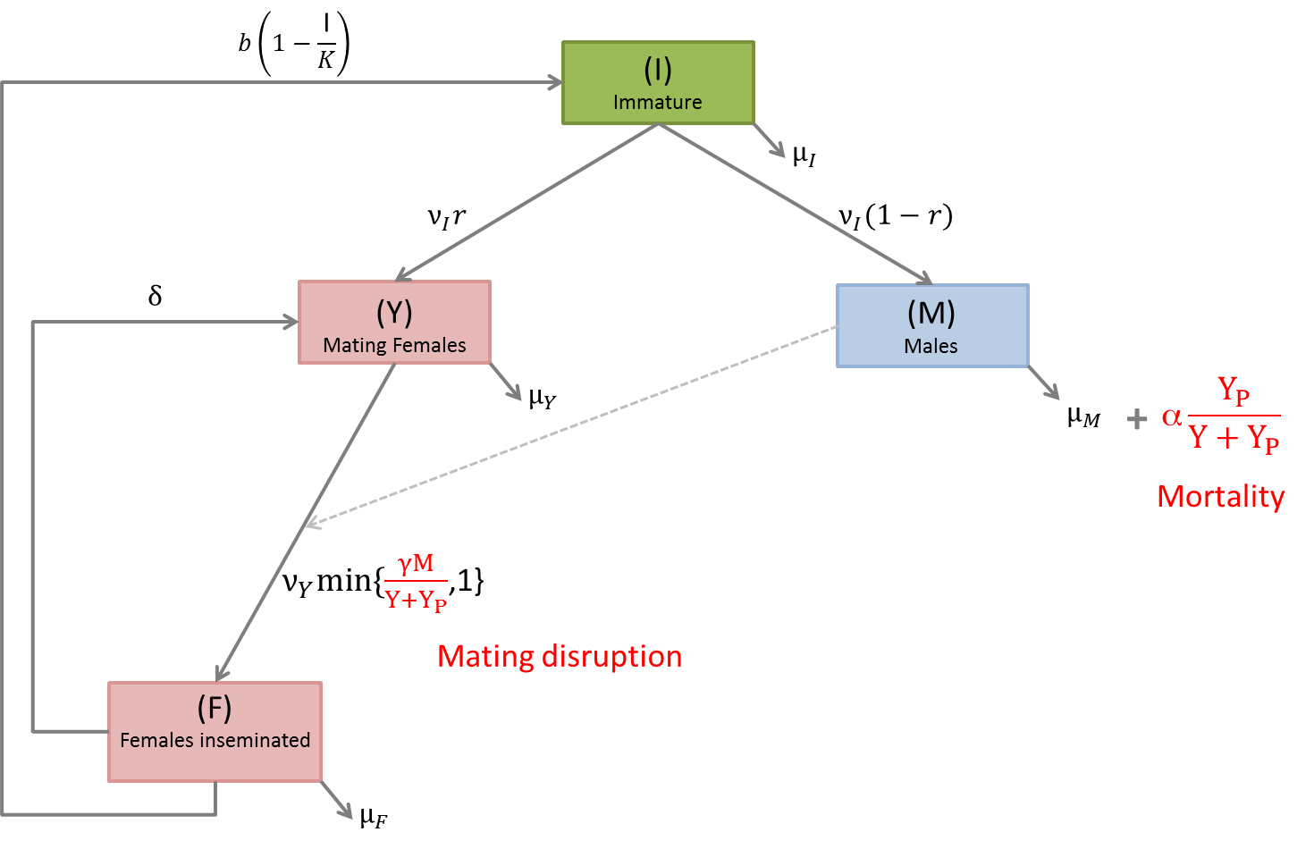
The parameter α𝛼\alpha represents the death or capture rate for the fraction YPY+YPsubscript𝑌𝑃𝑌subscript𝑌𝑃\displaystyle\frac{Y_{P}}{Y+Y_{P}} of the males which are attracted by the lures. The flow diagram is represented in Figure 2 which yields the following system of ODEs:

{dIdt=b(1IK)F(νI+μI)I,dYdt=rνIIνYmin{γMY+YP,1}Y+δFμYY,dFdt=νYmin{γMY+YP,1}YδFμFF,dMdt=(1r)νII(μM+αYPY+YP)M.cases𝑑𝐼𝑑𝑡𝑏1𝐼𝐾𝐹subscript𝜈𝐼subscript𝜇𝐼𝐼missing-subexpressionmissing-subexpressionmissing-subexpression𝑑𝑌𝑑𝑡𝑟subscript𝜈𝐼𝐼subscript𝜈𝑌𝛾𝑀𝑌subscript𝑌𝑃1𝑌𝛿𝐹subscript𝜇𝑌𝑌missing-subexpressionmissing-subexpressionmissing-subexpression𝑑𝐹𝑑𝑡subscript𝜈𝑌𝛾𝑀𝑌subscript𝑌𝑃1𝑌𝛿𝐹subscript𝜇𝐹𝐹missing-subexpressionmissing-subexpressionmissing-subexpression𝑑𝑀𝑑𝑡1𝑟subscript𝜈𝐼𝐼subscript𝜇𝑀𝛼subscript𝑌𝑃𝑌subscript𝑌𝑃𝑀\left\{\begin{array}[]{lcl}\frac{dI}{dt}&=&b\left(1-\frac{I}{K}\right)F-\left(\nu_{I}+\mu_{I}\right)I,\\ &&\\ \frac{dY}{dt}&=&r\nu_{I}I-\nu_{Y}\min\{\frac{\gamma M}{Y+Y_{P}},1\}Y+\delta F-\mu_{Y}Y,\\ &&\\ \frac{dF}{dt}&=&\nu_{Y}\min\{\frac{\gamma M}{Y+Y_{P}},1\}Y-\delta F-\mu_{F}F,\\ &&\\ \frac{dM}{dt}&=&(1-r)\nu_{I}I-(\mu_{M}+\alpha\frac{Y_{P}}{Y+Y_{P}})M.\end{array}\right. (17)
Refer to caption
Figure 2: Control model using mating disruption and trapping.

3.3 Theoretical analysis of the control model

The aim of this section is to investigate the existence of equilibria of model (17) and their asymptotic properties. First we consider the model in the male abundance state and in the male scarcity state independently. Then we draw conclusions for the general model.

3.3.1 Properties of the equilibria in the male abundance region (γM>Y+YP𝛾𝑀𝑌subscript𝑌𝑃\gamma M>Y+Y_{P})

The dynamics of the population in the male abundance region Y+YP<γM𝑌subscript𝑌𝑃𝛾𝑀Y+Y_{P}<\gamma M are governed by the following system of ODEs:

{dIdt=b(1IK)F(νI+μI)I,dYdt=rνIIνYY+δFμYY,dFdt=νYY(δ+μF)F,dMdt=(1r)νII(μM+αYPY+YP)M.cases𝑑𝐼𝑑𝑡𝑏1𝐼𝐾𝐹subscript𝜈𝐼subscript𝜇𝐼𝐼missing-subexpressionmissing-subexpressionmissing-subexpression𝑑𝑌𝑑𝑡𝑟subscript𝜈𝐼𝐼subscript𝜈𝑌𝑌𝛿𝐹subscript𝜇𝑌𝑌missing-subexpressionmissing-subexpressionmissing-subexpression𝑑𝐹𝑑𝑡subscript𝜈𝑌𝑌𝛿subscript𝜇𝐹𝐹missing-subexpressionmissing-subexpressionmissing-subexpression𝑑𝑀𝑑𝑡1𝑟subscript𝜈𝐼𝐼subscript𝜇𝑀𝛼subscript𝑌𝑃𝑌subscript𝑌𝑃𝑀\left\{\begin{array}[]{lcl}\frac{dI}{dt}&=&b\left(1-\frac{I}{K}\right)F-\left(\nu_{I}+\mu_{I}\right)I,\\ &&\\ \frac{dY}{dt}&=&r\nu_{I}I-\nu_{Y}Y+\delta F-\mu_{Y}Y,\\ &&\\ \frac{dF}{dt}&=&\nu_{Y}Y-(\delta+\mu_{F})F,\\ &&\\ \frac{dM}{dt}&=&(1-r)\nu_{I}I-(\mu_{M}+\alpha\frac{Y_{P}}{Y+Y_{P}})M.\end{array}\right. (18)

We note that the first three equations in (18) as in (2) are the same, while the fourth equation in both systems can be decoupled. Then, using exactly the same method as in Theorem 1 we obtain the following theorem.

Theorem 4.
  • a)

    The system of ODEs (18) defines a positive dynamical system on +4superscriptsubscript4\mathbb{R}_{+}^{4}.

  • b)

    Under assumptions (14) and (15), the system has a positive equilibrium EE#=(I,Y,F,M#(YP))T𝐸superscript𝐸#superscriptsuperscript𝐼superscript𝑌superscript𝐹superscript𝑀#subscript𝑌𝑃𝑇EE^{\#}=(I^{*},Y^{*},F^{*},M^{\#}(Y_{P}))^{T}, where

    M#(YP)=(1r)νI(Y+YP)μM(Y+YP)+αYPI=M1+αYPμM(Y+YP),superscript𝑀#subscript𝑌𝑃1𝑟subscript𝜈𝐼superscript𝑌subscript𝑌𝑃subscript𝜇𝑀superscript𝑌subscript𝑌𝑃𝛼subscript𝑌𝑃superscript𝐼superscript𝑀1𝛼subscript𝑌𝑃subscript𝜇𝑀superscript𝑌subscript𝑌𝑃M^{\#}(Y_{P})=\frac{(1-r)\nu_{I}(Y^{*}+Y_{P})}{\mu_{M}(Y^{*}+Y_{P})+\alpha Y_{P}}I^{*}=\frac{M^{*}}{1+\frac{\alpha Y_{P}}{\mu_{M}(Y^{*}+Y_{P})}},

    which is globally asymptotically stable on +4{x+4:I=Y=F=0}subscriptsuperscript4conditional-set𝑥subscriptsuperscript4𝐼𝑌𝐹0\mathbb{R}^{4}_{+}\setminus\{x\in\mathbb{R}^{4}_{+}:I=Y=F=0\}.

The equilibrium EE#𝐸superscript𝐸#EE^{\#} is an equilibrium of (17) if and only if

Y+YP<γM#(YP)superscript𝑌subscript𝑌𝑃𝛾superscript𝑀#subscript𝑌𝑃Y^{*}+Y_{P}<\gamma M^{\#}(Y_{P})

or, equivalently,

YP<YP:=γMY1+αμM=1μM+α(γ(1r)νIrνI(δ+μF)μM(νY+μY)(δ+μF)δνY)(11𝒩0)K.subscript𝑌𝑃superscriptsubscript𝑌𝑃assign𝛾superscript𝑀superscript𝑌1𝛼subscript𝜇𝑀1subscript𝜇𝑀𝛼𝛾1𝑟subscript𝜈𝐼𝑟subscript𝜈𝐼𝛿subscript𝜇𝐹subscript𝜇𝑀subscript𝜈𝑌subscript𝜇𝑌𝛿subscript𝜇𝐹𝛿subscript𝜈𝑌11subscript𝒩0𝐾Y_{P}<Y_{P}^{*}:=\frac{\gamma M^{*}-Y^{*}}{1+\frac{\alpha}{\mu_{M}}}=\frac{1}{\mu_{M}+\alpha}\left(\gamma(1-r)\nu_{I}-\frac{r\nu_{I}(\delta+\mu_{F})\mu_{M}}{(\nu_{Y}+\mu_{Y})(\delta+\mu_{F})-\delta\nu_{Y}}\right)\left(1-\frac{1}{\mathcal{N}_{0}}\right)K. (19)

The threshold value YPsuperscriptsubscript𝑌𝑃Y_{P}^{*} determines the minimal level of control below which the control has essentially no effect on an established pest population. More precisely, the effect is limited to reducing the number of males, while all other compartments remain in their natural equilibrium.

3.3.2 Properties of the equilibria in the male scarcity region (γM<Y+YP𝛾𝑀𝑌subscript𝑌𝑃\gamma M<Y+Y_{P})

In the region of male scarcity γMY+YP𝛾𝑀𝑌subscript𝑌𝑃\gamma M\leq Y+Y_{P} the dynamics of the population is governed by the system:

{dIdt=b(1IK)F(νI+μI)I,dYdt=rνIIνYγMYY+YP+δFμYY,dFdt=νYγMYY+YP(δ+μF)F,dMdt=(1r)νII(μM+αYPY+YP)M.cases𝑑𝐼𝑑𝑡𝑏1𝐼𝐾𝐹subscript𝜈𝐼subscript𝜇𝐼𝐼missing-subexpressionmissing-subexpressionmissing-subexpression𝑑𝑌𝑑𝑡𝑟subscript𝜈𝐼𝐼subscript𝜈𝑌𝛾𝑀𝑌𝑌subscript𝑌𝑃𝛿𝐹subscript𝜇𝑌𝑌missing-subexpressionmissing-subexpressionmissing-subexpression𝑑𝐹𝑑𝑡subscript𝜈𝑌𝛾𝑀𝑌𝑌subscript𝑌𝑃𝛿subscript𝜇𝐹𝐹missing-subexpressionmissing-subexpressionmissing-subexpression𝑑𝑀𝑑𝑡1𝑟subscript𝜈𝐼𝐼subscript𝜇𝑀𝛼subscript𝑌𝑃𝑌subscript𝑌𝑃𝑀\left\{\begin{array}[]{lcl}\frac{dI}{dt}&=&b\left(1-\frac{I}{K}\right)F-\left(\nu_{I}+\mu_{I}\right)I,\\ &&\\ \frac{dY}{dt}&=&r\nu_{I}I-\nu_{Y}\frac{\gamma MY}{Y+Y_{P}}+\delta F-\mu_{Y}Y,\\ &&\\ \frac{dF}{dt}&=&\nu_{Y}\frac{\gamma MY}{Y+Y_{P}}-(\delta+\mu_{F})F,\\ &&\\ \frac{dM}{dt}&=&(1-r)\nu_{I}I-(\mu_{M}+\alpha\frac{Y_{P}}{Y+Y_{P}})M.\end{array}\right. (20)

The following theorem exhibits different behaviours of the model depending on the value of YPsubscript𝑌𝑃Y_{P} which can be interpreted as the effort of the mating disruption control.

Theorem 5.
  • a)

    The system of ODEs (20) defines a positive dynamical system on +4subscriptsuperscript4\mathbb{R}^{4}_{+}.

  • b)

    TE is an asymptotically stable equilibrium of this system.

  • c)

    There exists a threshold value YPsuperscriptsubscript𝑌𝑃absentY_{P}^{**} of YPsubscript𝑌𝑃Y_{P} such that

    • i)

      if YP>YPsubscript𝑌𝑃superscriptsubscript𝑌𝑃absentY_{P}>Y_{P}^{**} the only equilibrium of the system on +4subscriptsuperscript4\mathbb{R}^{4}_{+} is TE;

    • ii)

      if 0<YP<YP0subscript𝑌𝑃superscriptsubscript𝑌𝑃absent0<Y_{P}<Y_{P}^{**} the system has three biologically relevant equilibria on +4subscriptsuperscript4\mathbb{R}^{4}_{+}, TE and two positive equilibria.

Proof.

a) The local existence of the solutions of (20) follows from the fact that the right hand side is Lipschitz continuous in +4subscriptsuperscript4\mathbb{R}^{4}_{+}. To obtain global existence it is enough to show that every solution is bounded. This can be proved directly, but it also follows from the upper approximation of the solutions discussed in the proof of Theorem 8. Hence, it is omitted here.

b) It is clear that TE=(0,0,0,0)T𝑇𝐸superscript0000𝑇TE=(0,0,0,0)^{T} is an equilibrium. The Jacobian of the right hand side of system (20) is

𝒥h(x)=((νI+μI+bFK)0b(1IK)0rνI(νYγMYP(Y+YP)2+μY)δνYγY(Y+YP)0νYγMYP(Y+YP)2(μF+δ)νYγY(Y+YP)(1r)νIαYP(Y+YP)2M0(μM+αYPY+YP)),subscript𝒥𝑥subscript𝜈𝐼subscript𝜇𝐼𝑏𝐹𝐾0𝑏1𝐼𝐾0𝑟subscript𝜈𝐼subscript𝜈𝑌𝛾𝑀subscript𝑌𝑃superscript𝑌subscript𝑌𝑃2subscript𝜇𝑌𝛿subscript𝜈𝑌𝛾𝑌𝑌subscript𝑌𝑃0subscript𝜈𝑌𝛾𝑀subscript𝑌𝑃superscript𝑌subscript𝑌𝑃2subscript𝜇𝐹𝛿subscript𝜈𝑌𝛾𝑌𝑌subscript𝑌𝑃1𝑟subscript𝜈𝐼𝛼subscript𝑌𝑃superscript𝑌subscript𝑌𝑃2𝑀0subscript𝜇𝑀𝛼subscript𝑌𝑃𝑌subscript𝑌𝑃\mathcal{J}_{h}(x)=\left(\begin{array}[]{cccc}-\left(\nu_{I}+\mu_{I}+b\frac{F}{K}\right)&0&b\left(1-\frac{I}{K}\right)&0\\ r\nu_{I}&-(\nu_{Y}\gamma M\frac{Y_{P}}{(Y+Y_{P})^{2}}+\mu_{Y})&\delta&-\nu_{Y}\gamma\frac{Y}{(Y+Y_{P})}\\ 0&\nu_{Y}\gamma M\frac{Y_{P}}{(Y+Y_{P})^{2}}&-(\mu_{F}+\delta)&\nu_{Y}\gamma\frac{Y}{(Y+Y_{P})}\\ (1-r)\nu_{I}&\frac{\alpha Y_{P}}{(Y+Y_{P})^{2}}M&0&-(\mu_{M}+\alpha\frac{Y_{P}}{Y+Y_{P}})\\ \end{array}\right), (21)

thus,

𝒥h(TE)=((νI+μI)0b0rνIμYδ000(δ+μF)0(1r)νI00(μM+α)).subscript𝒥𝑇𝐸subscript𝜈𝐼subscript𝜇𝐼0𝑏0𝑟subscript𝜈𝐼subscript𝜇𝑌𝛿000𝛿subscript𝜇𝐹01𝑟subscript𝜈𝐼00subscript𝜇𝑀𝛼\mathcal{J}_{h}(TE)=\left(\begin{array}[]{cccc}-\left(\nu_{I}+\mu_{I}\right)&0&b&0\\ r\nu_{I}&-\mu_{Y}&\delta&0\\ 0&0&-(\delta+\mu_{F})&0\\ (1-r)\nu_{I}&0&0&-(\mu_{M}+\alpha)\\ \end{array}\right). (22)

Its eigenvalues are equal to its diagonal entries and are all negative real values. Hence TE𝑇𝐸TE is asymptotically stable.

c) Setting dIdt=0𝑑𝐼𝑑𝑡0\frac{dI}{dt}=0 in (20) yields

F=νI+μIb(1IK)I.𝐹subscript𝜈𝐼subscript𝜇𝐼𝑏1𝐼𝐾𝐼F=\frac{\nu_{I}+\mu_{I}}{b\left(1-\frac{I}{K}\right)}I.

Then, from dMdt=0𝑑𝑀𝑑𝑡0\frac{dM}{dt}=0, we have

M=(1r)νIμM+αYPY+YPI.𝑀1𝑟subscript𝜈𝐼subscript𝜇𝑀𝛼subscript𝑌𝑃𝑌subscript𝑌𝑃𝐼M=\frac{(1-r)\nu_{I}}{\mu_{M}+\alpha\frac{Y_{P}}{Y+Y_{P}}}I.

Further, considering that dYdt+dFdt=0𝑑𝑌𝑑𝑡𝑑𝐹𝑑𝑡0\frac{dY}{dt}+\frac{dF}{dt}=0, we deduce

Y=rνIIμFFμY=(rνIμYμF(νI+μI)μYb(1IK))I=ϕ(I)μYb(1IK)I.𝑌𝑟subscript𝜈𝐼𝐼subscript𝜇𝐹𝐹subscript𝜇𝑌𝑟subscript𝜈𝐼subscript𝜇𝑌subscript𝜇𝐹subscript𝜈𝐼subscript𝜇𝐼subscript𝜇𝑌𝑏1𝐼𝐾𝐼italic-ϕ𝐼subscript𝜇𝑌𝑏1𝐼𝐾𝐼Y=\frac{r\nu_{I}I-\mu_{F}F}{\mu_{Y}}=\left(\frac{r\nu_{I}}{\mu_{Y}}-\frac{\mu_{F}(\nu_{I}+\mu_{I})}{\mu_{Y}b\left(1-\frac{I}{K}\right)}\right)I=\frac{\phi(I)}{\mu_{Y}b\left(1-\frac{I}{K}\right)}I.

with ϕ(I)=rνIb(1IK)μF(νI+μI)italic-ϕ𝐼𝑟subscript𝜈𝐼𝑏1𝐼𝐾subscript𝜇𝐹subscript𝜈𝐼subscript𝜇𝐼\phi(I)=r\nu_{I}b(1-\frac{I}{K})-\mu_{F}(\nu_{I}+\mu_{I}). Now, we use dFdt=0𝑑𝐹𝑑𝑡0\frac{dF}{dt}=0,

dFdt=νYγMY+YPY(δ+μF)F=νYγ(1r)νIIμM(Y+YP)+αYPϕ(I)μYb(1IK)I(δ+μF)νI+μIb(1IK)I=0.𝑑𝐹𝑑𝑡subscript𝜈𝑌𝛾𝑀𝑌subscript𝑌𝑃𝑌𝛿subscript𝜇𝐹𝐹subscript𝜈𝑌𝛾1𝑟subscript𝜈𝐼𝐼subscript𝜇𝑀𝑌subscript𝑌𝑃𝛼subscript𝑌𝑃italic-ϕ𝐼subscript𝜇𝑌𝑏1𝐼𝐾𝐼𝛿subscript𝜇𝐹subscript𝜈𝐼subscript𝜇𝐼𝑏1𝐼𝐾𝐼0\frac{dF}{dt}=\frac{\nu_{Y}\gamma M}{Y+Y_{P}}Y-(\delta+\mu_{F})F=\frac{\nu_{Y}\gamma(1-r)\nu_{I}I}{\mu_{M}(Y+Y_{P})+\alpha Y_{P}}\frac{\phi(I)}{\mu_{Y}b\left(1-\frac{I}{K}\right)}I-(\delta+\mu_{F})\frac{\nu_{I}+\mu_{I}}{b\left(1-\frac{I}{K}\right)}I=0.

Thus by substituting the expressions of Y𝑌Y, F𝐹F and M𝑀M, we have

νYγ(1r)νIIμMY+(μM+α)YPϕ(I)μYb(1IK)I(δ+μF)νI+μIb(1IK)I=0(νYγ(1r)νIϕ(I)μYb(1IK)I)=(δ+μF)(νI+μI)b(1IK)(μMY+(μM+α)YP)(νYγ(1r)νIϕ(I)μYb(1IK)I(δ+μF)(νI+μI)(μM)b(1IK)ϕ(I)μYb(1IK))=(δ+μF)(νI+μI)(μM+α)YPb(1IK).missing-subexpressionsubscript𝜈𝑌𝛾1𝑟subscript𝜈𝐼𝐼subscript𝜇𝑀𝑌subscript𝜇𝑀𝛼subscript𝑌𝑃italic-ϕ𝐼subscript𝜇𝑌𝑏1𝐼𝐾𝐼𝛿subscript𝜇𝐹subscript𝜈𝐼subscript𝜇𝐼𝑏1𝐼𝐾𝐼0missing-subexpressionmissing-subexpressionsubscript𝜈𝑌𝛾1𝑟subscript𝜈𝐼italic-ϕ𝐼subscript𝜇𝑌𝑏1𝐼𝐾𝐼𝛿subscript𝜇𝐹subscript𝜈𝐼subscript𝜇𝐼𝑏1𝐼𝐾subscript𝜇𝑀𝑌subscript𝜇𝑀𝛼subscript𝑌𝑃missing-subexpressionmissing-subexpressionsubscript𝜈𝑌𝛾1𝑟subscript𝜈𝐼italic-ϕ𝐼subscript𝜇𝑌𝑏1𝐼𝐾𝐼𝛿subscript𝜇𝐹subscript𝜈𝐼subscript𝜇𝐼subscript𝜇𝑀𝑏1𝐼𝐾italic-ϕ𝐼subscript𝜇𝑌𝑏1𝐼𝐾𝛿subscript𝜇𝐹subscript𝜈𝐼subscript𝜇𝐼subscript𝜇𝑀𝛼subscript𝑌𝑃𝑏1𝐼𝐾\begin{array}[]{rl}&\frac{\nu_{Y}\gamma(1-r)\nu_{I}I}{\mu_{M}Y+(\mu_{M}+\alpha)Y_{P}}\frac{\phi(I)}{\mu_{Y}b\left(1-\frac{I}{K}\right)}I-(\delta+\mu_{F})\frac{\nu_{I}+\mu_{I}}{b\left(1-\frac{I}{K}\right)}I=0\\ &\\ \Leftrightarrow&\left(\nu_{Y}\gamma(1-r)\nu_{I}\frac{\phi(I)}{\mu_{Y}b\left(1-\frac{I}{K}\right)}I\right)=\frac{(\delta+\mu_{F})(\nu_{I}+\mu_{I})}{b\left(1-\frac{I}{K}\right)}(\mu_{M}Y+(\mu_{M}+\alpha)Y_{P})\\ &\\ \Leftrightarrow&\left(\nu_{Y}\gamma(1-r)\nu_{I}\frac{\phi(I)}{\mu_{Y}b\left(1-\frac{I}{K}\right)}I-\frac{(\delta+\mu_{F})(\nu_{I}+\mu_{I})(\mu_{M})}{b\left(1-\frac{I}{K}\right)}\frac{\phi(I)}{\mu_{Y}b\left(1-\frac{I}{K}\right)}\right)=\frac{(\delta+\mu_{F})(\nu_{I}+\mu_{I})(\mu_{M}+\alpha)Y_{P}}{b\left(1-\frac{I}{K}\right)}.\end{array}

Multiplying both side by μYb2(1IK)2subscript𝜇𝑌superscript𝑏2superscript1𝐼𝐾2\mu_{Y}b^{2}(1-\frac{I}{K})^{2}, we obtain an equation for I𝐼I in the form

ψ(I):=Iξ(I)ϕ(I)=η(YP,I),assign𝜓𝐼𝐼𝜉𝐼italic-ϕ𝐼𝜂subscript𝑌𝑃𝐼\psi(I):=I\xi(I)\phi(I)=\eta(Y_{P},I), (23)

where

ξ(I)=νYγ(1r)νIb(1IK)(δ+μF)(νI+μI)μM,𝜉𝐼subscript𝜈𝑌𝛾1𝑟subscript𝜈𝐼𝑏1𝐼𝐾𝛿subscript𝜇𝐹subscript𝜈𝐼subscript𝜇𝐼subscript𝜇𝑀\xi(I)=\nu_{Y}\gamma(1-r)\nu_{I}b\left(1-\frac{I}{K}\right)-(\delta+\mu_{F})(\nu_{I}+\mu_{I})\mu_{M}, (24)
ϕ(I)=rνIb(1IK)μF(νI+μI),italic-ϕ𝐼𝑟subscript𝜈𝐼𝑏1𝐼𝐾subscript𝜇𝐹subscript𝜈𝐼subscript𝜇𝐼\phi(I)=r\nu_{I}b\left(1-\frac{I}{K}\right)-\mu_{F}(\nu_{I}+\mu_{I}), (25)

and

η(YP,I)=μY(δ+μF)(νI+μI)(μM+α)b(1IK)YP.𝜂subscript𝑌𝑃𝐼subscript𝜇𝑌𝛿subscript𝜇𝐹subscript𝜈𝐼subscript𝜇𝐼subscript𝜇𝑀𝛼𝑏1𝐼𝐾subscript𝑌𝑃\eta(Y_{P},I)=\mu_{Y}(\delta+\mu_{F})(\nu_{I}+\mu_{I})(\mu_{M}+\alpha)b\left(1-\frac{I}{K}\right)Y_{P}. (26)

Therefore, the non-trivial equilibria of (20) are of the form

YMDsubscript𝑌𝑀𝐷\displaystyle Y_{MD} =\displaystyle= (rνIμYμF(νI+μI)μYb(1IMDK))IMD,𝑟subscript𝜈𝐼subscript𝜇𝑌subscript𝜇𝐹subscript𝜈𝐼subscript𝜇𝐼subscript𝜇𝑌𝑏1subscript𝐼𝑀𝐷𝐾subscript𝐼𝑀𝐷\displaystyle\left(\frac{r\nu_{I}}{\mu_{Y}}-\frac{\mu_{F}(\nu_{I}+\mu_{I})}{\mu_{Y}b\left(1-\frac{I_{MD}}{K}\right)}\right)I_{MD}, (27)
FMDsubscript𝐹𝑀𝐷\displaystyle F_{MD} =\displaystyle= νI+μIb(1IMDK)IMD,subscript𝜈𝐼subscript𝜇𝐼𝑏1subscript𝐼𝑀𝐷𝐾subscript𝐼𝑀𝐷\displaystyle\frac{\nu_{I}+\mu_{I}}{b\left(1-\frac{I_{MD}}{K}\right)}I_{MD}, (28)
MMDsubscript𝑀𝑀𝐷\displaystyle M_{MD} =\displaystyle= (1r)νIμM+αYPYMD+YPIMD.1𝑟subscript𝜈𝐼subscript𝜇𝑀𝛼subscript𝑌𝑃subscript𝑌𝑀𝐷subscript𝑌𝑃subscript𝐼𝑀𝐷\displaystyle\frac{(1-r)\nu_{I}}{\mu_{M}+\alpha\frac{Y_{P}}{Y_{MD}+Y_{P}}}I_{MD}. (29)

with IMDsubscript𝐼𝑀𝐷I_{MD} a positive root of (23). Further, we note that to ensure YMD>0subscript𝑌𝑀𝐷0Y_{MD}>0, it follows from (27) that IMDsubscript𝐼𝑀𝐷I_{MD} must satisfy the condition

IMD<K(1μF(νI+μI)rνIb).subscript𝐼𝑀𝐷𝐾1subscript𝜇𝐹subscript𝜈𝐼subscript𝜇𝐼𝑟subscript𝜈𝐼𝑏I_{MD}<K\left(1-\frac{\mu_{F}(\nu_{I}+\mu_{I})}{r\nu_{I}b}\right). (30)

Thus, to obtain biologically viable equilibria, IMDsubscript𝐼𝑀𝐷I_{MD} must belong to the interval [0,K(1μF(νI+μI)rνIb)]0𝐾1subscript𝜇𝐹subscript𝜈𝐼subscript𝜇𝐼𝑟subscript𝜈𝐼𝑏\left[0,K\left(1-\frac{\mu_{F}(\nu_{I}+\mu_{I})}{r\nu_{I}b}\right)\right].

The roots of (23) correspond to the values of I𝐼I where the graph of the cubic polynomial ψ𝜓\psi and the straight line η(YP,)𝜂subscript𝑌𝑃\eta(Y_{P},\cdot) intersect. It is clear that, the straight line η(YP,)𝜂subscript𝑌𝑃\eta(Y_{P},\cdot) intersects the I𝐼I-axis at I=K𝐼𝐾I=K. From the factorization of ψ(I)𝜓𝐼\psi(I) in (23), it is clear that the roots of ψ𝜓\psi are

I0=0,I1=K(1(δ+μF)(νI+μI)μMνYγ(1r)νIb), and I2=K(1μF(νI+μI)rνIb).formulae-sequencesubscript𝐼00formulae-sequencesubscript𝐼1𝐾1𝛿subscript𝜇𝐹subscript𝜈𝐼subscript𝜇𝐼subscript𝜇𝑀subscript𝜈𝑌𝛾1𝑟subscript𝜈𝐼𝑏 and subscript𝐼2𝐾1subscript𝜇𝐹subscript𝜈𝐼subscript𝜇𝐼𝑟subscript𝜈𝐼𝑏I_{0}=0,\quad I_{1}=K\left(1-\frac{(\delta+\mu_{F})(\nu_{I}+\mu_{I})\mu_{M}}{\nu_{Y}\gamma(1-r)\nu_{I}b}\right),\textrm{ and }I_{2}=K\left(1-\frac{\mu_{F}(\nu_{I}+\mu_{I})}{r\nu_{I}b}\right). (31)

Note that the the roots I1subscript𝐼1I_{1} and respectively, I2subscript𝐼2I_{2}, are positive and smaller than K𝐾K, i.e.

0<I1,I2<K,formulae-sequence0subscript𝐼1subscript𝐼2𝐾0<I_{1},I_{2}<K,

provided

(δ+μF)(νI+μI)μMνYγ(1r)νIb<1,𝛿subscript𝜇𝐹subscript𝜈𝐼subscript𝜇𝐼subscript𝜇𝑀subscript𝜈𝑌𝛾1𝑟subscript𝜈𝐼𝑏1\frac{(\delta+\mu_{F})(\nu_{I}+\mu_{I})\mu_{M}}{\nu_{Y}\gamma(1-r)\nu_{I}b}<1, (32)

and respectively,

μF(νI+μI)rνIb<1.subscript𝜇𝐹subscript𝜈𝐼subscript𝜇𝐼𝑟subscript𝜈𝐼𝑏1\frac{\mu_{F}(\nu_{I}+\mu_{I})}{r\nu_{I}b}<1. (33)

Inequality (32) is satisfied under assumptions (15) and (14), and inequality (33) is equivalent to 𝒩0>1subscript𝒩01\mathcal{N}_{0}>1, that is, to (14). Therefore, under assumptions (14) and (15), we have that

I1,I2[0,K].subscript𝐼1subscript𝐼20𝐾I_{1},I_{2}\in[0,K].

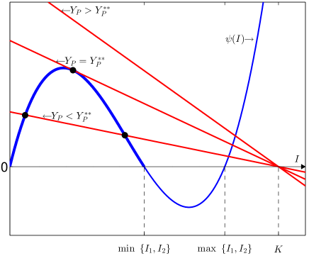
Therefore, the graph of the cubic polynomial ψ𝜓\psi is as given on Figure 3.

Refer to caption
Figure 3: Intersections between the graphs of η(YP,)𝜂subscript𝑌𝑃\eta(Y_{P},\cdot) (in red) and ψ𝜓\psi (in blue) for different values of YPsubscript𝑌𝑃Y_{P}. The black dots represent the intersection points on the interval [0,min{I1,I2}]0subscript𝐼1subscript𝐼2[0,\min\{I_{1},I_{2}\}].

Considering the inequality (30), only points of intersection of the straight line η(YP,)𝜂subscript𝑌𝑃\eta(Y_{P},\cdot) with the section of the graph of ψ𝜓\psi for 0Imin{I1,I2}0𝐼subscript𝐼1subscript𝐼20\leq I\leq\min\{I_{1},I_{2}\}, indicated by a thicker line on Figure 3, are of relevance to the equilibria of the model. Let us note that ψ𝜓\psi is independent of YPsubscript𝑌𝑃Y_{P} while the gradient of the line η𝜂\eta is a multiple of YPsubscript𝑌𝑃Y_{P}. We denote by YPsuperscriptsubscript𝑌𝑃absentY_{P}^{**} the value of YPsubscript𝑌𝑃Y_{P} such that the line η(YP,)𝜂subscript𝑌𝑃\eta(Y_{P},\cdot) is tangent to the indicated section of the graph of ψ𝜓\psi, see Figure 3. Then it is clear that for YP>YPsubscript𝑌𝑃superscriptsubscript𝑌𝑃absentY_{P}>Y_{P}^{**} there is no intersection between η(YP,)𝜂subscript𝑌𝑃\eta(Y_{P},\cdot) and ψ𝜓\psi on [0,min{I1,I2}]0subscript𝐼1subscript𝐼2\left[0,\min\{I_{1},I_{2}\}\right] while if 0<YP<YP0subscript𝑌𝑃superscriptsubscript𝑌𝑃absent0<Y_{P}<Y_{P}^{**} there are two such points of intersection. This proves items (i) and (ii) in c).

The next step in this analysis is to merge the results in Theorem 4 for system (18) and the results in Theorem 5 for the system (20) in order to obtain results for the model (17) which is actually our interest.

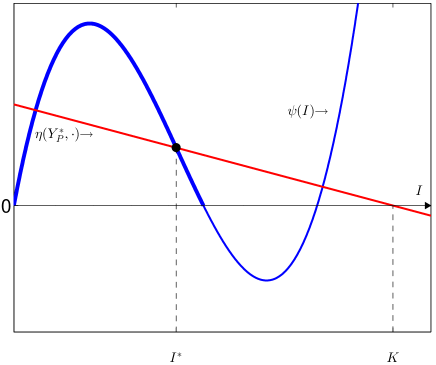
Let IMD(1)subscriptsuperscript𝐼1𝑀𝐷I^{(1)}_{MD} and IMD(2)subscriptsuperscript𝐼2𝑀𝐷I^{(2)}_{MD},IMD(1)<IMD(2)subscriptsuperscript𝐼1𝑀𝐷subscriptsuperscript𝐼2𝑀𝐷I^{(1)}_{MD}<I^{(2)}_{MD}, be the roots of (23) when 0<YP<YP0subscript𝑌𝑃superscriptsubscript𝑌𝑃absent0<Y_{P}<Y_{P}^{**} and denote the respective equilibria by EEMD(1)𝐸subscriptsuperscript𝐸1𝑀𝐷EE^{(1)}_{MD} and EEMD(2)𝐸subscriptsuperscript𝐸2𝑀𝐷EE^{(2)}_{MD}. First we show that EE#=EEMD(2)𝐸superscript𝐸#𝐸subscriptsuperscript𝐸2𝑀𝐷EE^{\#}=EE^{(2)}_{MD} when YP=YPsubscript𝑌𝑃superscriptsubscript𝑌𝑃Y_{P}=Y_{P}^{*}. Indeed, YPsuperscriptsubscript𝑌𝑃Y_{P}^{*} is selected in such way that γMY+YP=1𝛾superscript𝑀superscript𝑌subscriptsuperscript𝑌𝑃1\displaystyle\frac{\gamma M^{*}}{Y^{*}+Y^{*}_{P}}=1. Then, the right hand sides of (18) and (20) are the same at EE#𝐸superscript𝐸#EE^{\#}. This implies that EE#𝐸superscript𝐸#EE^{\#} is an equilibrium of (20).

Refer to caption
Figure 4: Intersections between the graphs of η(YP,)𝜂superscriptsubscript𝑌𝑃\eta(Y_{P}^{*},\cdot) (in red) and ψ𝜓\psi (in blue). The black dot represent the intersection for I=I𝐼superscript𝐼I=I^{*}.

One can see from Figure 4 that for 0<YP<YP0subscript𝑌𝑃superscriptsubscript𝑌𝑃0<Y_{P}<Y_{P}^{*}, we have

IMD(1)<I<IMD(2),subscriptsuperscript𝐼1𝑀𝐷superscript𝐼subscriptsuperscript𝐼2𝑀𝐷I^{(1)}_{MD}<I^{*}<I^{(2)}_{MD}, (34)

and for YP<YP<YPsuperscriptsubscript𝑌𝑃subscript𝑌𝑃superscriptsubscript𝑌𝑃absentY_{P}^{*}<Y_{P}<Y_{P}^{**}, we have

IMD(1)<IMD(2)<I.subscriptsuperscript𝐼1𝑀𝐷subscriptsuperscript𝐼2𝑀𝐷superscript𝐼I^{(1)}_{MD}<I^{(2)}_{MD}<I^{*}. (35)

We investigate when the equilibria of (17) are biologically relevant, that is when they belong to the male scarcity region. We have

YMD+YPγMMDsubscript𝑌𝑀𝐷subscript𝑌𝑃𝛾subscript𝑀𝑀𝐷\displaystyle Y_{MD}+Y_{P}-\gamma M_{MD} (36)
=YMD+YPγ(1r)νIμM+αYPYMD+YPIMDabsentsubscript𝑌𝑀𝐷subscript𝑌𝑃𝛾1𝑟subscript𝜈𝐼subscript𝜇𝑀𝛼subscript𝑌𝑃subscript𝑌𝑀𝐷subscript𝑌𝑃subscript𝐼𝑀𝐷\displaystyle=Y_{MD}+Y_{P}-\gamma\frac{(1-r)\nu_{I}}{\mu_{M}+\alpha\frac{Y_{P}}{Y_{MD}+Y_{P}}}I_{MD}
=μMYMD+μYYP+αYPγ(1r)νIμM+αYPYMD+YPIMD.absentsubscript𝜇𝑀subscript𝑌𝑀𝐷subscript𝜇𝑌subscript𝑌𝑃𝛼subscript𝑌𝑃𝛾1𝑟subscript𝜈𝐼subscript𝜇𝑀𝛼subscript𝑌𝑃subscript𝑌𝑀𝐷subscript𝑌𝑃subscript𝐼𝑀𝐷\displaystyle=\frac{\mu_{M}Y_{MD}+\mu_{Y}Y_{P}+\alpha Y_{P}-\gamma(1-r)\nu_{I}}{\mu_{M}+\alpha\frac{Y_{P}}{Y_{MD}+Y_{P}}}I_{MD}.
=(μMμM+αYPYMD+YP(rνIμYμF(νI+μI)μY(1IMDK))γ(1r)νI)IMD+(μM+α)YP.absentsubscript𝜇𝑀subscript𝜇𝑀𝛼subscript𝑌𝑃subscript𝑌𝑀𝐷subscript𝑌𝑃𝑟subscript𝜈𝐼subscript𝜇𝑌subscript𝜇𝐹subscript𝜈𝐼subscript𝜇𝐼subscript𝜇𝑌1subscript𝐼𝑀𝐷𝐾𝛾1𝑟subscript𝜈𝐼subscript𝐼𝑀𝐷subscript𝜇𝑀𝛼subscript𝑌𝑃\displaystyle=\left(\frac{\mu_{M}}{\mu_{M}+\alpha\frac{Y_{P}}{Y_{MD}+Y_{P}}}\left(\frac{r\nu_{I}}{\mu_{Y}}-\frac{\mu_{F}(\nu_{I}+\mu_{I})}{\mu_{Y}\left(1-\frac{I_{MD}}{K}\right)}\right)-\gamma(1-r)\nu_{I}\right)I_{MD}+(\mu_{M}+\alpha)Y_{P}.

Let YP<YP<YPsuperscriptsubscript𝑌𝑃subscript𝑌𝑃superscriptsubscript𝑌𝑃absentY_{P}^{*}<Y_{P}<Y_{P}^{**}. Then using also (35) we have

YMD+YPγMMDsubscript𝑌𝑀𝐷subscript𝑌𝑃𝛾subscript𝑀𝑀𝐷\displaystyle Y_{MD}+Y_{P}-\gamma M_{MD}
μMμM+αYPYMD+YP(rνIμYμF(νI+μI)μY(1IK)γ(1r)νI)IMD+(μM+α)YPabsentsubscript𝜇𝑀subscript𝜇𝑀𝛼subscript𝑌𝑃subscript𝑌𝑀𝐷subscript𝑌𝑃𝑟subscript𝜈𝐼subscript𝜇𝑌subscript𝜇𝐹subscript𝜈𝐼subscript𝜇𝐼subscript𝜇𝑌1superscript𝐼𝐾𝛾1𝑟subscript𝜈𝐼subscript𝐼𝑀𝐷subscript𝜇𝑀𝛼subscript𝑌𝑃\displaystyle\geq\frac{\mu_{M}}{\mu_{M}+\alpha\frac{Y_{P}}{Y_{MD}+Y_{P}}}\left(\frac{r\nu_{I}}{\mu_{Y}}-\frac{\mu_{F}(\nu_{I}+\mu_{I})}{\mu_{Y}\left(1-\frac{I^{*}}{K}\right)}-\gamma(1-r)\nu_{I}\right)I_{MD}+(\mu_{M}+\alpha)Y_{P} (37)
=((μMrνI(δ+μF)νYμF+μYμF+δμY)γ(1r)νI)IMD+(μM+α)YP(using (19))absentsubscript𝜇𝑀𝑟subscript𝜈𝐼𝛿subscript𝜇𝐹subscript𝜈𝑌subscript𝜇𝐹subscript𝜇𝑌subscript𝜇𝐹𝛿subscript𝜇𝑌𝛾1𝑟subscript𝜈𝐼subscript𝐼𝑀𝐷subscript𝜇𝑀𝛼subscript𝑌𝑃(using (19))\displaystyle=\left(\left(\mu_{M}\frac{r\nu_{I}(\delta+\mu_{F})}{\nu_{Y}\mu_{F}+\mu_{Y}\mu_{F}+\delta\mu_{Y}}\right)-\gamma(1-r)\nu_{I}\right)I_{MD}+(\mu_{M}+\alpha)Y_{P}\quad\textrm{(using (\ref{YPstar}))}
=(μM+α)YPIIMD+(μM+α)YPabsentsubscript𝜇𝑀𝛼superscriptsubscript𝑌𝑃superscript𝐼subscript𝐼𝑀𝐷subscript𝜇𝑀𝛼subscript𝑌𝑃\displaystyle=-(\mu_{M}+\alpha)\frac{Y_{P}^{*}}{I^{*}}I_{MD}+(\mu_{M}+\alpha)Y_{P}
=μM+αI(YPIYPIMD)>0.absentsubscript𝜇𝑀𝛼superscript𝐼subscript𝑌𝑃superscript𝐼superscriptsubscript𝑌𝑃subscript𝐼𝑀𝐷0\displaystyle=\frac{\mu_{M}+\alpha}{I^{*}}\left(Y_{P}I^{*}-Y_{P}^{*}I_{MD}\right)>0.

Therefore, in this case EEMD(1)𝐸subscriptsuperscript𝐸1𝑀𝐷EE^{(1)}_{MD} and EEMD(2)𝐸subscriptsuperscript𝐸2𝑀𝐷EE^{(2)}_{MD} are both in the male scarcity region. Hence, they are also equilibria of (17).

If YP<YPsubscript𝑌𝑃superscriptsubscript𝑌𝑃Y_{P}<Y_{P}^{*} and IMD>Isubscript𝐼𝑀𝐷superscript𝐼I_{MD}>I^{*}, considering (34), then using the same method as in (37) we obtain

YP+YMDγMMD<0.subscript𝑌𝑃subscript𝑌𝑀𝐷𝛾subscript𝑀𝑀𝐷0Y_{P}+Y_{MD}-\gamma M_{MD}<0. (38)

Therefore, EEMD(2)𝐸subscriptsuperscript𝐸2𝑀𝐷EE^{(2)}_{MD} is not in the male scarcity region. Hence, it is not an equilibrium of (17).

Taking into consideration the above results regarding EEMD(1)𝐸subscriptsuperscript𝐸1𝑀𝐷EE^{(1)}_{MD} and EEMD(2)𝐸subscriptsuperscript𝐸2𝑀𝐷EE^{(2)}_{MD} we obtain the following theorem for the model (17).

Theorem 6.

Let YP>0subscript𝑌𝑃0Y_{P}>0. The following holds for model (17):

  • a)

    TE𝑇𝐸TE is an asymptotically stable equilibrium.

  • b)

    If 0<YP<YP0subscript𝑌𝑃superscriptsubscript𝑌𝑃0<Y_{P}<Y_{P}^{*} there are two positive equilibria EEMD(1)𝐸subscriptsuperscript𝐸1𝑀𝐷EE^{(1)}_{MD} and EE#𝐸superscript𝐸#EE^{\#}, where EE#𝐸superscript𝐸#EE^{\#} is asymptotically stable.

  • c)

    If YP<YP<YPsuperscriptsubscript𝑌𝑃subscript𝑌𝑃superscriptsubscript𝑌𝑃absentY_{P}^{*}<Y_{P}<Y_{P}^{**} there are two positive equilibria EEMD(1)𝐸subscriptsuperscript𝐸1𝑀𝐷EE^{(1)}_{MD} and EEMD(2)𝐸subscriptsuperscript𝐸2𝑀𝐷EE^{(2)}_{MD}.

  • d)

    If YP>YPsubscript𝑌𝑃superscriptsubscript𝑌𝑃absentY_{P}>Y_{P}^{**} there is no positive equilibrium.

Obtaining theoretically the stability properties of the equilibria EEMD(1)𝐸subscriptsuperscript𝐸1𝑀𝐷EE^{(1)}_{MD} and EEMD(2)𝐸subscriptsuperscript𝐸2𝑀𝐷EE^{(2)}_{MD} is not easy considering the complexity of the system. The numerical simulations indicate that EEMD(1)𝐸subscriptsuperscript𝐸1𝑀𝐷EE^{(1)}_{MD} is unstable while EEMD(2)𝐸subscriptsuperscript𝐸2𝑀𝐷EE^{(2)}_{MD} is asymptotically stable, and that the equilibria are the only invariant set of the system on 4+subscriptsuperscript4\mathbb{R}^{+}_{4}. Further, when YP>YPsubscript𝑌𝑃superscriptsubscript𝑌𝑃absentY_{P}>Y_{P}^{**}, TE𝑇𝐸TE is globally asymptotically stable. The equilibria and their properties are presented on the bifurcation diagram in Figure 5. The equilibrium values of Y+F𝑌𝐹Y+F are given as function of the bifurcation parameter YPsubscript𝑌𝑃Y_{P}. The solid line represents stable equilibria, while the dotted line represents unstable equilibria.
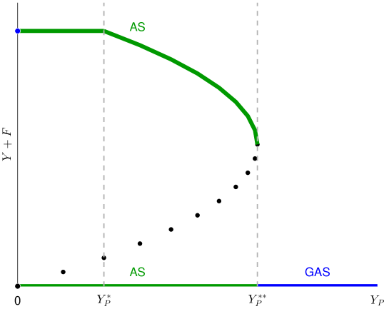
Refer to caption
Figure 5: Bifurcation diagram of the values of Y+F𝑌𝐹Y+F at equilibrium with respect to the values of YPsubscript𝑌𝑃Y_{P} for system (17).

3.3.3 Global asymptotic stability of the trivial equilibrium for sufficiently large YPsubscript𝑌𝑃Y_{P}

Theorem 6 shows that for YP<YPsubscript𝑌𝑃superscriptsubscript𝑌𝑃absentY_{P}<Y_{P}^{**} the insect population persists at substantial endemic level. Hence, the numerically observed global asymptotic stability of TE𝑇𝐸TE for YP>YPsubscript𝑌𝑃superscriptsubscript𝑌𝑃absentY_{P}>Y_{P}^{**} is of significant practical importance. This section deals with the mathematical proof of this result. More precisely, we will establish global asymptotic stability of TE𝑇𝐸TE under slightly stronger condition YP>Y~Psubscript𝑌𝑃superscriptsubscript~𝑌𝑃absentY_{P}>\tilde{Y}_{P}^{**} where Y~P>YPsuperscriptsubscript~𝑌𝑃absentsuperscriptsubscript𝑌𝑃absent\tilde{Y}_{P}^{**}>Y_{P}^{**}. We also show that Y~Psuperscriptsubscript~𝑌𝑃absent\tilde{Y}_{P}^{**} is a close approximation for YPsuperscriptsubscript𝑌𝑃absentY_{P}^{**}.

The asymptotic analysis for system (17) cannot be conducted in the same way as for the other systems considered so far, since it is not a monotone system. More precisely due to the term νYγMY+YPYsubscript𝜈𝑌𝛾𝑀𝑌subscript𝑌𝑃𝑌\displaystyle-\nu_{Y}\frac{\gamma M}{Y+Y_{P}}Y in the equation for the Y𝑌Y compartment, the right hand side of (17) is not quasi-monotone. In order to obtain the practically important result mentioned above, we consider an auxiliary system which is monotone and provides upper bounds for the solutions of (17). The system is obtained by removing the mentioned term in the second equation and replacing min{γMY+YP,1}𝛾𝑀𝑌subscript𝑌𝑃1\displaystyle\min\{\frac{\gamma M}{Y+Y_{P}},1\} by γMY+YP𝛾𝑀𝑌subscript𝑌𝑃\displaystyle\frac{\gamma M}{Y+Y_{P}} in the third equation. In vector form it is given as

dxdt=h~(x),𝑑𝑥𝑑𝑡~𝑥\frac{dx}{dt}=\tilde{h}(x), (39)

where x=(I,Y,F,M)T𝑥superscript𝐼𝑌𝐹𝑀𝑇x=(I,Y,F,M)^{T} and

h~(x)=(b(1IK)F(νI+μI)IrνIIμYY+δFνYγMY+YPYδFμFF(1r)νII(μM+αYPY+YP)M).~𝑥𝑏1𝐼𝐾𝐹subscript𝜈𝐼subscript𝜇𝐼𝐼𝑟subscript𝜈𝐼𝐼subscript𝜇𝑌𝑌𝛿𝐹subscript𝜈𝑌𝛾𝑀𝑌subscript𝑌𝑃𝑌𝛿𝐹subscript𝜇𝐹𝐹1𝑟subscript𝜈𝐼𝐼subscript𝜇𝑀𝛼subscript𝑌𝑃𝑌subscript𝑌𝑃𝑀\tilde{h}(x)=\left(\begin{array}[]{c}b\left(1-\frac{I}{K}\right)F-\left(\nu_{I}+\mu_{I}\right)I\\ r\nu_{I}I-\mu_{Y}Y+\delta F\\ \nu_{Y}\frac{\gamma M}{Y+Y_{P}}Y-\delta F-\mu_{F}F\\ (1-r)\nu_{I}I-(\mu_{M}+\alpha\frac{Y_{P}}{Y+Y_{P}})M\end{array}\right). (40)
Theorem 7.
  • a)

    The system of ODEs (39) defines a positive dynamical system on +4subscriptsuperscript4\mathbb{R}^{4}_{+}.

  • b)

    TE is asymptotically stable equilibrium.

  • c)

    There exists a threshold value Y~Psuperscriptsubscript~𝑌𝑃absent\tilde{Y}_{P}^{**} such that

    • i)

      if YP>Y~Psubscript𝑌𝑃superscriptsubscript~𝑌𝑃absentY_{P}>\tilde{Y}_{P}^{**}, TE is globally asymptotically stable on +4subscriptsuperscript4\mathbb{R}^{4}_{+};

    • ii)

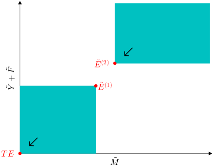
      if 0<YP<Y~P0subscript𝑌𝑃superscriptsubscript~𝑌𝑃absent0<Y_{P}<\tilde{Y}_{P}^{**}, the system has three equilibria, TE𝑇𝐸TE and two positive equilibria E~(1)superscript~𝐸1\tilde{E}^{(1)} and E~(2)superscript~𝐸2\tilde{E}^{(2)} such that E~(1)<E~(2)superscript~𝐸1superscript~𝐸2\tilde{E}^{(1)}<\tilde{E}^{(2)}. The basin of attraction of TE𝑇𝐸TE contains the set {x+4:0x<E~(1)}conditional-set𝑥subscriptsuperscript40𝑥superscript~𝐸1\{x\in\mathbb{R}^{4}_{+}:0\leq x<\tilde{E}^{(1)}\}. The basin of attraction of E~(2)superscript~𝐸2\tilde{E}^{(2)} contains the set {x+4:xE~(2),IK}conditional-set𝑥subscriptsuperscript4formulae-sequence𝑥superscript~𝐸2𝐼𝐾\{x\in\mathbb{R}^{4}_{+}:x\geq\tilde{E}^{(2)},I\leq K\}.

Proof.

a) and b) are proved similarly to a) and b) in Theorem 5.

c) Setting the first, second and fourth component of h~~\tilde{h} to zero, we have

Y=rνII+δFμY,F=νI+μIb(1IK)I,M=(1r)νIμMY+(μM+α)YPI.formulae-sequence𝑌𝑟subscript𝜈𝐼𝐼𝛿𝐹subscript𝜇𝑌formulae-sequence𝐹subscript𝜈𝐼subscript𝜇𝐼𝑏1𝐼𝐾𝐼𝑀1𝑟subscript𝜈𝐼subscript𝜇𝑀𝑌subscript𝜇𝑀𝛼subscript𝑌𝑃𝐼Y=\frac{r\nu_{I}I+\delta F}{\mu_{Y}},\quad F=\frac{\nu_{I}+\mu_{I}}{b\left(1-\frac{I}{K}\right)}I,\quad M=\frac{(1-r)\nu_{I}}{\mu_{M}Y+(\mu_{M}+\alpha)Y_{P}}I.

Setting the third component of h~~\tilde{h} to zero and substituting the expressions for Y𝑌Y, F𝐹F and M𝑀M above, we obtain an equation for I𝐼I in the form

ψ~(I):=Iξ(I)ϕ~(I)=η(YP,I).assign~𝜓𝐼𝐼𝜉𝐼~italic-ϕ𝐼𝜂subscript𝑌𝑃𝐼\tilde{\psi}(I):=I\xi(I)\tilde{\phi}(I)=\eta(Y_{P},I). (41)

where ξ(I)𝜉𝐼\xi(I) and η(YP,I)𝜂subscript𝑌𝑃𝐼\eta(Y_{P},I) are the linear expression given in (24) and (26) and

ϕ~(I)=rνIb(1IK)+δ(νI+μI).~italic-ϕ𝐼𝑟subscript𝜈𝐼𝑏1𝐼𝐾𝛿subscript𝜈𝐼subscript𝜇𝐼\tilde{\phi}(I)=r\nu_{I}b\left(1-\frac{I}{K}\right)+\delta(\nu_{I}+\mu_{I}). (42)

Therefore the non-trivial equilibria of (39) are of the form

Y~~𝑌\displaystyle\tilde{Y} =\displaystyle= 1μY(rνI+δ(νI+μI)b(1I~K))I~,1subscript𝜇𝑌𝑟subscript𝜈𝐼𝛿subscript𝜈𝐼subscript𝜇𝐼𝑏1~𝐼𝐾~𝐼\displaystyle\frac{1}{\mu_{Y}}\left(r\nu_{I}+\frac{\delta(\nu_{I}+\mu_{I})}{b\left(1-\frac{\tilde{I}}{K}\right)}\right)\tilde{I},
F~~𝐹\displaystyle\tilde{F} =\displaystyle= νI+μIb(1I~K)I~,subscript𝜈𝐼subscript𝜇𝐼𝑏1~𝐼𝐾~𝐼\displaystyle\frac{\nu_{I}+\mu_{I}}{b\left(1-\frac{\tilde{I}}{K}\right)}\tilde{I}, (43)
M~~𝑀\displaystyle\tilde{M} =\displaystyle= (1r)νIμM+αYPY~+YPI~,1𝑟subscript𝜈𝐼subscript𝜇𝑀𝛼subscript𝑌𝑃~𝑌subscript𝑌𝑃~𝐼\displaystyle\frac{(1-r)\nu_{I}}{\mu_{M}+\alpha\frac{Y_{P}}{\tilde{Y}+Y_{P}}}\tilde{I},

with I~~𝐼\tilde{I} a positive root of (42). The roots of (42) correspond to the values of I𝐼I where the graph of the cubic polynomial ψ~~𝜓\tilde{\psi} and the straight line η(YP,)𝜂subscript𝑌𝑃\eta(Y_{P},\cdot) intersect. It is clear that the straight line η(YP,)𝜂subscript𝑌𝑃\eta(Y_{P},\cdot) intersects the I𝐼I axis at I=K𝐼𝐾I=K. Note that the state where I𝐼I greater is than K𝐾K is not sustainable, and therefore not biologically relevant. From the factorization of ψ~~𝜓\tilde{\psi} in (42), it is clear that I0subscript𝐼0I_{0} and I1subscript𝐼1I_{1} given in (31) and

I~2=(1+δ(νI+μI)rνIb)Ksubscript~𝐼21𝛿subscript𝜈𝐼subscript𝜇𝐼𝑟subscript𝜈𝐼𝑏𝐾\tilde{I}_{2}=\left(1+\frac{\delta(\nu_{I}+\mu_{I})}{r\nu_{I}b}\right)K (44)

are roots of ψ~~𝜓\tilde{\psi}. Clearly, we have

0<I1<K<I~2.0subscript𝐼1𝐾subscript~𝐼20<I_{1}<K<\tilde{I}_{2}.

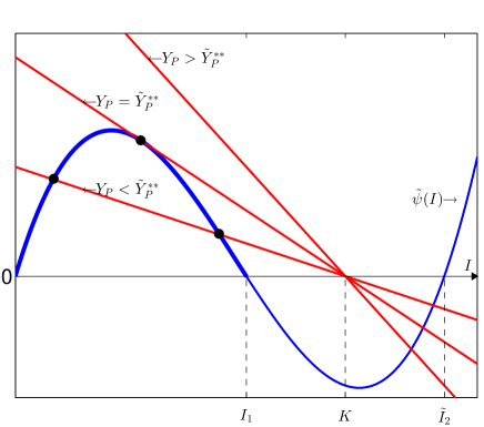
Therefore, the graph of the cubic polynomial ψ~~𝜓\tilde{\psi} is as given in Figure 6.

Refer to caption
Figure 6: Intersections between the graphs of η(YP,)𝜂subscript𝑌𝑃\eta(Y_{P},\cdot) (in red) and ψ𝜓\psi (in blue) for different values of YPsubscript𝑌𝑃Y_{P}. The black dots represent the intersection points on the interval [0,I1]0subscript𝐼1[0,I_{1}].

Considering the inequalities (30) and (3.3.3), only the points of intersection of the straight line η(YP,)𝜂subscript𝑌𝑃\eta(Y_{P},\cdot) with the section of the graph of ψ~~𝜓\tilde{\psi} for 0<I<I10𝐼subscript𝐼10<I<I_{1} are of relevance to the equilibria of the model. Note that ψ~~𝜓\tilde{\psi} is independent of YPsubscript𝑌𝑃Y_{P} while the gradient of η(YP,)𝜂subscript𝑌𝑃\eta(Y_{P},\cdot) is a multiple of YPsubscript𝑌𝑃Y_{P}. We denote by Y~Psuperscriptsubscript~𝑌𝑃absent\tilde{Y}_{P}^{**} the value of YPsubscript𝑌𝑃Y_{P} such that the line η𝜂\eta is tangent to the indicated section of the graph of ψ~~𝜓\tilde{\psi}, see Figure 6. Then, it is clear that for YP>Y~Psubscript𝑌𝑃superscriptsubscript~𝑌𝑃absentY_{P}>\tilde{Y}_{P}^{**} there is no intersection between η(YP,)𝜂subscript𝑌𝑃\eta(Y_{P},\cdot) and ψ~~𝜓\tilde{\psi} on [0,I1]0subscript𝐼1[0,I_{1}] while if 0<YP<Y~P0subscript𝑌𝑃superscriptsubscript~𝑌𝑃absent0<Y_{P}<\tilde{Y}_{P}^{**} there are two such points of intersection.

i) Let YP>Y~Psubscript𝑌𝑃superscriptsubscript~𝑌𝑃absentY_{P}>\tilde{Y}_{P}^{**}. Consider the point

y~q=(K1μY(rνI+δνYγ(1r)νI(δ+μF)μM)qνYγ(1r)νI(δ+μF)μMq(1r)νIμMq),subscript~𝑦𝑞𝐾1subscript𝜇𝑌𝑟subscript𝜈𝐼𝛿subscript𝜈𝑌𝛾1𝑟subscript𝜈𝐼𝛿subscript𝜇𝐹subscript𝜇𝑀𝑞subscript𝜈𝑌𝛾1𝑟subscript𝜈𝐼𝛿subscript𝜇𝐹subscript𝜇𝑀𝑞1𝑟subscript𝜈𝐼subscript𝜇𝑀𝑞\tilde{y}_{q}=\left(\begin{array}[]{c}K\\ \frac{1}{\mu_{Y}}\left(r\nu_{I}+\frac{\delta\nu_{Y}\gamma(1-r)\nu_{I}}{(\delta+\mu_{F})\mu_{M}}\right)q\\ \frac{\nu_{Y}\gamma(1-r)\nu_{I}}{(\delta+\mu_{F})\mu_{M}}q\\ \frac{(1-r)\nu_{I}}{\mu_{M}}q\\ \end{array}\right), (45)

where q,qKformulae-sequence𝑞𝑞𝐾q\in\mathbb{R},q\geq K. It is easy to see that h~(y~q)0~subscript~𝑦𝑞0\tilde{h}(\tilde{y}_{q})\leq 0. Then by Theorem 13, TE𝑇𝐸TE is GAS on [0,y~q]0subscript~𝑦𝑞[\textbf{0},\tilde{y}_{q}]. Therefore, TE𝑇𝐸TE is GAS on ΩK=qK[0,y~q]subscriptΩ𝐾subscript𝑞𝐾0subscript~𝑦𝑞\Omega_{K}=\cup_{q\geq K}[\textbf{0},\tilde{y}_{q}] as well. Similarly to Theorem 1, ΩKsubscriptΩ𝐾\Omega_{K} is an absorbing set. Hence TE𝑇𝐸TE is GAS on +4subscriptsuperscript4\mathbb{R}^{4}_{+}.

ii) Let 0<YP<Y~P0subscript𝑌𝑃superscriptsubscript~𝑌𝑃absent0<Y_{P}<\tilde{Y}_{P}^{**}. Denote the two equilibria by E~(j)=(I~(j),Y~(j),F~(j),M~(j))Tsuperscript~𝐸𝑗superscriptsuperscript~𝐼𝑗superscript~𝑌𝑗superscript~𝐹𝑗superscript~𝑀𝑗𝑇\tilde{E}^{(j)}=(\tilde{I}^{(j)},\tilde{Y}^{(j)},\tilde{F}^{(j)},\tilde{M}^{(j)})^{T}, j=1,2𝑗12j=1,2, where I~(1)<I~(2)superscript~𝐼1superscript~𝐼2\tilde{I}^{(1)}<\tilde{I}^{(2)}. Since Y~~𝑌\tilde{Y}, F~~𝐹\tilde{F}, M~~𝑀\tilde{M} as given in (43) are increasing functions of I~~𝐼\tilde{I}, we have 0<E~(1)<E~(2)0superscript~𝐸1superscript~𝐸20<\tilde{E}^{(1)}<\tilde{E}^{(2)} (Figure 7).

Refer to caption
Figure 7: Positive invariant sets, when 0<YP<Y~P0subscript𝑌𝑃superscriptsubscript~𝑌𝑃absent0<Y_{P}<\tilde{Y}_{P}^{**}.

Considering y~qsubscript~𝑦𝑞\tilde{y}_{q} in (45) we have

h~(E~(2))=0h~(y~q).~superscript~𝐸20~subscript~𝑦𝑞\tilde{h}(\tilde{E}^{(2)})=0\leq\tilde{h}(\tilde{y}_{q}).

Then by Theorem 13 E~(2)superscript~𝐸2\tilde{E}^{(2)} is GAS on [E~(2),y~q]superscript~𝐸2subscript~𝑦𝑞[\tilde{E}^{(2)},\tilde{y}_{q}]. Therefore, E~(2)superscript~𝐸2\tilde{E}^{(2)} is GAS on qK[E~(2),y~q]={x+4:xE~(2),IK}subscript𝑞𝐾superscript~𝐸2subscript~𝑦𝑞conditional-set𝑥subscriptsuperscript4formulae-sequence𝑥superscript~𝐸2𝐼𝐾\cup_{q\geq K}[\tilde{E}^{(2)},\tilde{y}_{q}]=\{x\in\mathbb{R}^{4}_{+}:x\geq\tilde{E}^{(2)},I\leq K\}. We obtain the statements about the basin of attraction of TE𝑇𝐸TE by using Theorem 14. Indeed, TE𝑇𝐸TE being asymptotically stable, attracts some solutions initiated in [TE,E~(1)]𝑇𝐸superscript~𝐸1\displaystyle[TE,\tilde{E}^{(1)}]. Then it follows from Theorem 14 that all solutions initiated in {x+4:x<E~(1)}conditional-set𝑥subscriptsuperscript4𝑥superscript~𝐸1\{x\in\mathbb{R}^{4}_{+}:x<\tilde{E}^{(1)}\} converge to TE𝑇𝐸TE. ∎

The implication of Theorem 7 for the system (17) are stated in the following theorem which extends the results of Theorem 6.

Theorem 8.

Let YP>0subscript𝑌𝑃0Y_{P}>0. Then the following hold for the model (17).

  • a)

    If 0<YPY~P0subscript𝑌𝑃superscriptsubscript~𝑌𝑃absent0<Y_{P}\leq\tilde{Y}_{P}^{**}, then the basin of attraction of TE𝑇𝐸TE contains {x+4:x<E~(1)}conditional-set𝑥subscriptsuperscript4𝑥superscript~𝐸1\{x\in\mathbb{R}^{4}_{+}:x<\tilde{E}^{(1)}\}.

  • b)

    If YP>Y~Psubscript𝑌𝑃superscriptsubscript~𝑌𝑃absentY_{P}>\tilde{Y}_{P}^{**}, then TE𝑇𝐸TE is GAS on +4subscriptsuperscript4\mathbb{R}^{4}_{+}.

Proof.

Using Theorem 11 with x𝑥x being the solution of (39) and y𝑦y being the solution of (17) we obtain that any solution of (39) is an upper bound of the solution of (17) with the same initial point. This implies that the basin of attraction of TE𝑇𝐸TE as an equilibrium of (17) contains the sets indicated in Theorem 7 c) (i) and ii)), thus proving a) and b) respectively. ∎

Theorem 8 characterises the benefit from the control effort represented by YPsubscript𝑌𝑃Y_{P} as follows:

  • Increasing the effort YPsubscript𝑌𝑃Y_{P} in the range 0<YP<YP0subscript𝑌𝑃superscriptsubscript𝑌𝑃absent0<Y_{P}<Y_{P}^{**} does not lead to elimination of an established population. In fact, as shown on Figure 5, the reduction is not proportional to the effort. However, E~(1)superscript~𝐸1\tilde{E}^{(1)} increases at least linearly with I~(1)superscript~𝐼1\tilde{I}^{(1)}. Hence, increasing YPsubscript𝑌𝑃Y_{P} enlarges the basin of attraction of TE𝑇𝐸TE, providing better opportunity for controlling an invading population.

  • Effort YPsubscript𝑌𝑃Y_{P} stronger than Y~Psuperscriptsubscript~𝑌𝑃absent\tilde{Y}_{P}^{**} eliminates any established or invading population.

4 Numerical Simulation and Discussion

We use numerical simulations to illustrate the results of Theorems 6 and 8 and discuss the biological meaning of the results. The numerical simulations are done using the ode23tb solver of Matlab [30] which solves system of stiff ODEs using a trapezoidal rule and second order backward differentiation scheme (TR-BDF2) [6, 24]. The values of the parameters used for the numerical simulations are those of Table 1.

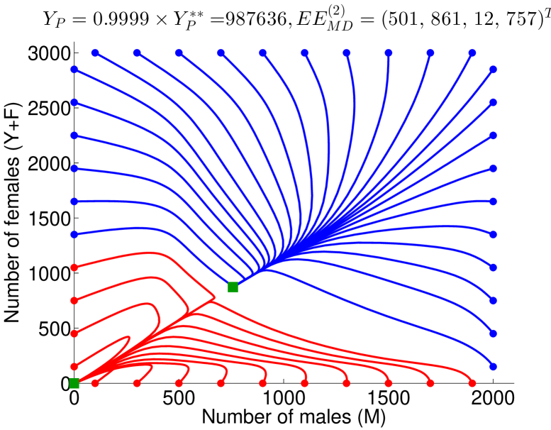
Using (5), we compute the basic offspring number, 𝒩0=122subscript𝒩0122\mathcal{N}_{0}=122. 𝒩0>1subscript𝒩01\mathcal{N}_{0}>1, therefore, the population establishes to the positive endemic equilibrium EE𝐸superscript𝐸EE^{*} which we have shown to be GAS on +4{TE}subscriptsuperscript4𝑇𝐸\mathbb{R}^{4}_{+}\setminus\{TE\} (Theorem 1 c)). Figure 8 represents the trajectories of a set of solutions of system (1), or equivalently system (17) with YP=0subscript𝑌𝑃0Y_{P}=0 and α=0𝛼0\alpha=0, in the M×(Y+F)𝑀𝑌𝐹M\times(Y+F) plane. The dots represent the points at which the solutions are initiated. The solutions initiated on +4{TE}subscriptsuperscript4𝑇𝐸\mathbb{R}^{4}_{+}\setminus\{TE\} all converge to the point EE=(992,319,1407,1498)T𝐸superscript𝐸superscript99231914071498𝑇EE^{*}=(992,319,1407,1498)^{T}, represented by the green square. Here, TE𝑇𝐸TE is also an equilibrium, but it is unstable (Theorem 1 c)), and therefore it is not represented in Figure 10.
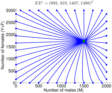
Refer to caption
Figure 8: Trajectories of a set solutions of system (1) in the M×(Y+F)𝑀𝑌𝐹M\times(Y+F)-plane initiated at the dots. The green square represents the stable equilibrium EE𝐸superscript𝐸EE^{*}.

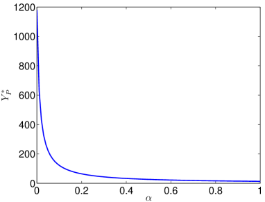
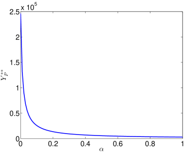
In the following, we confirm numerically the theoretical results of Theorems 6 and 8 with respect to the values of the mating disruption thresholds mentioned in those theorems, YPsuperscriptsubscript𝑌𝑃Y_{P}^{*} and YPsuperscriptsubscript𝑌𝑃absentY_{P}^{**}. We also investigate the impact of the trapping effort, α𝛼\alpha, on the population. Using (19) and solving numerically the system

{ψ(I)=η(YP,I)dψdI(I)=dηdI(YP,I)cases𝜓𝐼𝜂subscript𝑌𝑃𝐼missing-subexpressionmissing-subexpressionmissing-subexpression𝑑𝜓𝑑𝐼𝐼𝑑𝜂𝑑𝐼subscript𝑌𝑃𝐼\left\{\begin{array}[]{ccc}\psi(I)&=&\eta(Y_{P},I)\\ &&\\ \frac{d\psi}{dI}(I)&=&\frac{d\eta}{dI}(Y_{P},I)\end{array}\right.

with ψ𝜓\psi and η(YP,)𝜂subscript𝑌𝑃\eta(Y_{P},\cdot) as defined in (23), we obtain respectively the thresholds values YPsuperscriptsubscript𝑌𝑃Y_{P}^{*} and YPsuperscriptsubscript𝑌𝑃absentY_{P}^{**} as functions of α𝛼\alpha as represented in Figure 9.

Refer to caption
(a) YPsuperscriptsubscript𝑌𝑃Y_{P}^{*} as a function of α𝛼\alpha
Refer to caption
(b) YPsuperscriptsubscript𝑌𝑃absentY_{P}^{**} as a function of α𝛼\alpha
Figure 9: Mating disruption thresholds as function of the trapping parameter α𝛼\alpha.

One can observe that a small trapping effort reduces the mating disruption thresholds in a non-linear manner. Adding trapping to mating disruption allows to reduce the amount of the lure for equivalent control efficiency. In particular, for α=0𝛼0\alpha=0, we have YP=5673superscriptsubscript𝑌𝑃5673Y_{P}^{*}=5673 and YP=987735superscriptsubscript𝑌𝑃absent987735Y_{P}^{**}=987735, while for α=0.1𝛼0.1\alpha=0.1, we have YP=588superscriptsubscript𝑌𝑃588Y_{P}^{*}=588 and YP=102462superscriptsubscript𝑌𝑃absent102462Y_{P}^{**}=102462. Thus, increasing the trapping effort by 10%percent1010\% reduces both YPsuperscriptsubscript𝑌𝑃Y_{P}^{*} and YPsuperscriptsubscript𝑌𝑃absentY_{P}^{**} by 90%percent9090\%.

Figure 10 illustrates the trajectories of the solutions of system (17) when the mating disruption level is below the threshold YPsuperscriptsubscript𝑌𝑃Y_{P}^{*} for α=0𝛼0\alpha=0 and α=0.1𝛼0.1\alpha=0.1. The dots represent the initial points and the green squares represent the asymptotically stable equilibria. In this case, the system has one positive equilibrium, EE#𝐸superscript𝐸#EE^{\#} (Theorem 6 b)), with value given in the figure. One can observe that when there is no trapping, EE#=EE𝐸superscript𝐸#𝐸superscript𝐸EE^{\#}=EE^{*} (Figure 10 (a)). This means that the positive endemic equilibrium of the population is not affected by the control. When trapping occurs, we observe in Figure 10 (b) that the positive equilibrium is shifted to the left. In fact, the control allows to reduce the number of males but not sufficiently to disrupt the fertilisation of the females. Therefore, the control is not efficient on an established population as the number of females at equilibrium is not reduced.
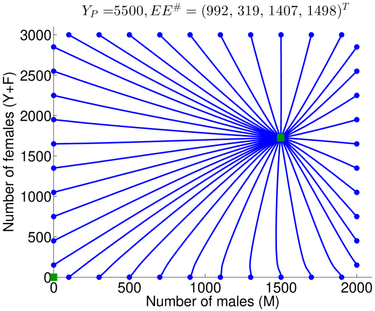
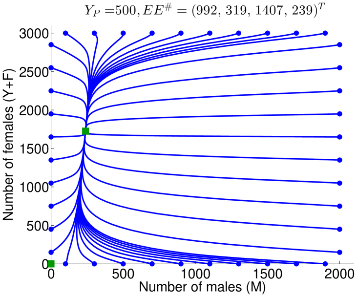
Refer to caption
(a) α=0𝛼0\alpha=0
Refer to caption
(b) α=0.1𝛼0.1\alpha=0.1
Figure 10: Trajectories of a set solutions of system (17) in the M×(Y+F)𝑀𝑌𝐹M\times(Y+F)-plane initiated at the dots. The green squares represent the asymptotically stable equilibria TE𝑇𝐸TE and EE#𝐸superscript𝐸#EE^{\#}.

However, when YP>0subscript𝑌𝑃0Y_{P}>0, TE𝑇𝐸TE is asymptotically stable, which means that a population can be controlled if it is small enough. Figure 11 (a), represents the basin of attraction of TE𝑇𝐸TE (the red dots) for a small population in the same setting as for the experiments in Figure 10 (a). We observe that there is a set of solutions, for which the initial population is small enough, that converge to TE𝑇𝐸TE, hence, a small population can be eradicated for YP>0subscript𝑌𝑃0Y_{P}>0. Further, as shown in Figure 11 (b), adding trapping (α=0.1𝛼0.1\alpha=0.1) with the same mating disruption effort as for Figure 11 (a), enlarges the basin of attraction of TE𝑇𝐸TE. In other words, for identical mating disruption effort, larger populations can be drawn to extinction when trapping occurs.
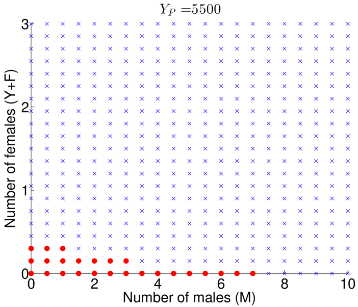
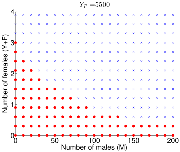
Refer to caption
(a) α=0𝛼0\alpha=0.
Refer to caption
(b) α=0.1𝛼0.1\alpha=0.1.
Figure 11: Effect of α𝛼\alpha on the basin of attraction of TE𝑇𝐸TE. The solutions initiated at the points represented by the red dots converge to TE𝑇𝐸TE while the blue crosses represent initial points for which the solution converges to EE#𝐸superscript𝐸#EE^{\#}.

In order to observe a reduction in the number of females, the mating disruption effort has to be increased above the threshold YPsuperscriptsubscript𝑌𝑃Y_{P}^{*}. This is the case in Figure 12 ((a) and (b)), where YP=0.9999×YP<YPsubscript𝑌𝑃0.9999superscriptsubscript𝑌𝑃absentsuperscriptsubscript𝑌𝑃Y_{P}=0.9999\times Y_{P}^{**}<Y_{P}^{*}, for α=0𝛼0\alpha=0 and α=0.1𝛼0.1\alpha=0.1, respectively. We can see that there is a positive asymptotically stable equilibrium, EEMD(2)𝐸subscriptsuperscript𝐸2𝑀𝐷EE^{(2)}_{MD} represented with a green square (Theorems 6 c)). The blue lines represent the trajectories of the solutions of (17) initiated at the blue points which converge to EEMD(2)𝐸subscriptsuperscript𝐸2𝑀𝐷EE^{(2)}_{MD}, while the red lines represent the trajectories of the solutions initiated at the red points which converge to TE𝑇𝐸TE. With YP>YPsubscript𝑌𝑃superscriptsubscript𝑌𝑃Y_{P}>Y_{P}^{*}, the number of females at equilibrium is reduced, however, the impact of the control is not proportional to the effort. Indeed comparing the experiments in Figures 10 and Figures 12, we observe that in order to reduce the number of females at equilibrium by 49%percent4949\%, the amount of the lure has to be increased by 17857%percent1785717857\% when α=0𝛼0\alpha=0 and by 20390%percent2039020390\% when α=0.1𝛼0.1\alpha=0.1.

Refer to caption
(a) α=0𝛼0\alpha=0.
Refer to caption
(b) α=0.1𝛼0.1\alpha=0.1
Figure 12: Trajectories of a set solutions of system (17) in the M×(Y+F)𝑀𝑌𝐹M\times(Y+F)-plane initiated at the dots. The green squares represent the asymptotically stable equilibria.

Further, comparing the red dots in Figure 11 and the red trajectories in Figure 12, we can see that the basin of attraction of the trivial equilibrium becomes larger as the value of YPsubscript𝑌𝑃Y_{P} increases.

Finally, YP>YPsubscript𝑌𝑃superscriptsubscript𝑌𝑃absentY_{P}>Y_{P}^{**} allows a full control of the population leading it to extinction no matter how big it is. In Figure 13, YPsubscript𝑌𝑃Y_{P} is above YPsuperscriptsubscript𝑌𝑃absentY_{P}^{**} by 0.01%percent0.010.01\%, and we can see that all the trajectories converge to TE𝑇𝐸TE. This shows the GAS nature of TE𝑇𝐸TE when YP>YPsubscript𝑌𝑃superscriptsubscript𝑌𝑃absentY_{P}>Y_{P}^{**}.

Refer to caption
(a) α=0𝛼0\alpha=0.
Refer to caption
(b) α=0.1𝛼0.1\alpha=0.1
Figure 13: Trajectories of a set solutions of system (17) in the M×(Y+F)𝑀𝑌𝐹M\times(Y+F)-plane initiated at the dots. The green squares represent the asymptotically stable equilibria.

Note that in Theorem 8, the GAS of TE𝑇𝐸TE is established for YP>Y~Psubscript𝑌𝑃superscriptsubscript~𝑌𝑃absentY_{P}>\tilde{Y}_{P}^{**}, however, we show numerically that the GAS property of TE𝑇𝐸TE holds for YP>YPsubscript𝑌𝑃superscriptsubscript𝑌𝑃absentY_{P}>Y_{P}^{**}. From Figure 14 we can see that the error between Y~Psuperscriptsubscript~𝑌𝑃absent\tilde{Y}_{P}^{**} and YPsuperscriptsubscript𝑌𝑃absentY_{P}^{**} is of order 104superscript10410^{4} which is small compared to the values of Y~Psuperscriptsubscript~𝑌𝑃absent\tilde{Y}_{P}^{**} and YPsuperscriptsubscript𝑌𝑃absentY_{P}^{**} which are of order 106superscript10610^{6}.

Refer to caption
Figure 14: Error between the thresholds Y~Psuperscriptsubscript~𝑌𝑃absent\tilde{Y}_{P}^{**} and YPsuperscriptsubscript𝑌𝑃absentY_{P}^{**} as function of α𝛼\alpha.

Conclusion and Perspectives

Controlling insect pest population in environmentally respectful manner is a main challenge in IPM programs. Mating disruption using female sex-pheromone based lures falls within IPM requirements as it is species specific and leaves no toxic residues in the produce grown. In this work, we build a generic model, governed by a system of ODEs to simulate the dynamics of a pest population and its response to mating disruption control with trapping. From the theoretical analysis of the model, we identify two threshold values of biological interest for the strength of the lure. The first threshold, YPsuperscriptsubscript𝑌𝑃Y_{P}^{*}, corresponds to a minimum amount of pheromone necessary for mating disruption to have an effect on the population. However, we show that the control can only be fully efficient, that is, drive an established population to extinction, for an amount of pheromone above a second threshold, YPsuperscriptsubscript𝑌𝑃absentY_{P}^{**}. We also show asymptotic stability of the trivial equilibrium, TE𝑇𝐸TE, whenever YP>0subscript𝑌𝑃0Y_{P}>0. In other words, a small amount of pheromone can be efficient on a very small population, like at invasion stage. Despite the different modelling approach and control method considered, similar results were found by Barclay and Mackauer [9], where a threshold for the size of the release of sterile males was identified, below which two positive equilibria were found, the larger one being stable and the smaller one being unstable, and above which SIT control is fully effective. These theoretical results are consistent with field observation, where the failure of mating disruption is often attributed to a wrong dosage of the pheromone and/or to an excessive population density [1, 31]. Further, we show that increasing the capture efficiency of the traps can reduce considerably these threshold values. From practical point of view this suggests that there is an optimal combination of the strength of the pheromone attractant and the capture efficiency of the traps to optimise the control of the pests in terms of population control and cost. These results support the conclusions of Yamanaka [37] stipulating that in the case where the lure used for mating disruption is strong enough, then additional trapping is not necessary, while otherwise, the author advise to rather focus the effort on the trapping efficiency. In a more realistic setting, this optimised control corresponds to an optimal setting of traps releasing the pheromone. Alternative approaches, such as individual based models (IBM), have been considered to study the impact of mating disruption, incorporating a spatial component where the attraction of males is governed by the pheromone plume [38], or by the effective attraction radius (EAR) which corresponds to the probability of finding the source [13]. A next step for this work is to add a spatial component to investigate how traps should be set, how many should be used, and how far from each other they should be positioned. Investigation on trap settings and their interactions have been studied in a parallel work dealing with parameter estimation [18] and extended in [2], where spatio-temporal trapping models are governed by advection-diffusion-reaction processes.

Another perspective is the validation of the model using field data obtained by Mark-Release-Recapture (MRR) experiments. MRR consists of releasing marked insects in the wild population and recapture them in traps. In such experiments, the number of insects released, as well as the position of the release and the position of the traps are known. Therefore, comparing the trapping data obtained with the model with those obtained using MRR experiments would enable us to validate the model. Then, following the protocol proposed in [2], unknown parameters of the model could be estimated.

Acknowledgements

This work has been supported by the French Ministry of Foreign Affairs and International Development and the South African National Research Foundation in the framework of the PHC PROTEA 2015 call. The support of the DST-NRF Centre of Excellence in Mathematical and Statistical Sciences (CoE-MaSS) towards this research is hereby acknowledged. Opinions expressed and conclusions arrived at, are those of the authors and are not necessarily to be attributed to the CoE.

Appendix A: Computation of the basic offspring number

The basic offspring number, sometimes called “net reproduction rate or ratio” [12], is defined as the expected number of females originated by a single female in a lifetime [32]. The computation can be done using a similar method as for the computation of the “basic reproduction number” in epidemiological model which determines the number if secondary infections produced by a single infectious individual [34, 17]. Let

  • i(x)subscript𝑖𝑥\mathcal{R}_{i}(x) be the rate of recruitment of new individuals in compartment i𝑖i,

  • 𝒯i+(x)superscriptsubscript𝒯𝑖𝑥\mathcal{T}_{i}^{+}(x) be the transfer of individuals into compartment i𝑖i, and

  • 𝒯i(x)superscriptsubscript𝒯𝑖𝑥\mathcal{T}_{i}^{-}(x) be the transfer of individuals out of compartment i𝑖i.

Our system can be written in the form:

x˙i=i(x)𝒯i(x),subscript˙𝑥𝑖subscript𝑖𝑥subscript𝒯𝑖𝑥\dot{x}_{i}=\mathcal{R}_{i}(x)-\mathcal{T}_{i}(x),

with

𝒯i=𝒯i(x)𝒯i+(x),subscript𝒯𝑖superscriptsubscript𝒯𝑖𝑥superscriptsubscript𝒯𝑖𝑥\mathcal{T}_{i}=\mathcal{T}_{i}^{-}(x)-\mathcal{T}_{i}^{+}(x),

i=1,..,4i=1,..,4. When γM>Y+YP𝛾𝑀𝑌subscript𝑌𝑃\gamma M>Y+Y_{P}, system (17) is reduced to system (18) and it can be written as

x˙=(x)𝒯(x),˙𝑥𝑥𝒯𝑥\dot{x}=\mathcal{R}(x)-\mathcal{T}(x),

with

(x)=(b(1IK)F000),𝑥𝑏1𝐼𝐾𝐹000\mathcal{R}(x)=\left(\begin{array}[]{c}b(1-\frac{I}{K})F\\ 0\\ 0\\ 0\\ \end{array}\right),

end

𝒯(x)=((νI+μI)I(νY+μY)YrνIIδF(δ+μF)FνYYμMM(1r)νII).𝒯𝑥subscript𝜈𝐼subscript𝜇𝐼𝐼subscript𝜈𝑌subscript𝜇𝑌𝑌𝑟subscript𝜈𝐼𝐼𝛿𝐹𝛿subscript𝜇𝐹𝐹subscript𝜈𝑌𝑌subscript𝜇𝑀𝑀1𝑟subscript𝜈𝐼𝐼\mathcal{T}(x)=\left(\begin{array}[]{c}(\nu_{I}+\mu_{I})I\\ (\nu_{Y}+\mu_{Y})Y-r\nu_{I}I-\delta F\\ (\delta+\mu_{F})F-\nu_{Y}Y\\ \mu_{M}M-(1-r)\nu_{I}I\\ \end{array}\right).

To obtain the next generation operator, we compute the Jacobian matrices of \mathcal{R} and 𝒯𝒯\mathcal{T}, respectively, Jsubscript𝐽J_{\mathcal{R}} and J𝒯subscript𝐽𝒯J_{\mathcal{T}}. Then, from [23, 34], the next generation operator is defined as RT1𝑅superscript𝑇1RT^{-1} where R=J(TE)𝑅subscript𝐽𝑇𝐸R=J_{\mathcal{R}}(TE) and T=J𝒯(TE)𝑇subscript𝐽𝒯𝑇𝐸T=J_{\mathcal{T}}(TE). Here, we have

R=(00b0000000000000), and T=(νI+μI000rνIνY+μYδ00νYδ+μF0(1r)νI00μM).formulae-sequence𝑅00𝑏0000000000000 and 𝑇subscript𝜈𝐼subscript𝜇𝐼000𝑟subscript𝜈𝐼subscript𝜈𝑌subscript𝜇𝑌𝛿00subscript𝜈𝑌𝛿subscript𝜇𝐹01𝑟subscript𝜈𝐼00subscript𝜇𝑀R=\left(\begin{array}[]{cccc}0&0&b&0\\ 0&0&0&0\\ 0&0&0&0\\ 0&0&0&0\\ \end{array}\right),\textrm{ and }\quad T=\left(\begin{array}[]{cccc}\nu_{I}+\mu_{I}&0&0&0\\ r\nu_{I}&\nu_{Y}+\mu_{Y}&-\delta&0\\ 0&-\nu_{Y}&\delta+\mu_{F}&0\\ (1-r)\nu_{I}&0&0&\mu_{M}\\ \end{array}\right).

The basic offspring number is obtained by computing the spectral radius of the next generation operator [34, 17]:

𝒩0=ρ(RT1)=brνIνY(μI+νI)((νY+μY)(δ+μF)δνY).subscript𝒩0𝜌𝑅superscript𝑇1𝑏𝑟subscript𝜈𝐼subscript𝜈𝑌subscript𝜇𝐼subscript𝜈𝐼subscript𝜈𝑌subscript𝜇𝑌𝛿subscript𝜇𝐹𝛿subscript𝜈𝑌\mathcal{N}_{0}=\rho(RT^{-1})=\frac{br\nu_{I}\nu_{Y}}{(\mu_{I}+\nu_{I})\left((\nu_{Y}+\mu_{Y})(\delta+\mu_{F})-\delta\nu_{Y}\right)}.

Appendix B: Computation of the endemic equilibrium

We seek for (I,Y,F,M)superscript𝐼superscript𝑌superscript𝐹superscript𝑀(I^{*},Y^{*},F^{*},M^{*}) such that

{dIdt=0,dYdt=0,dFdt=0,dMdt=0,cases𝑑superscript𝐼𝑑𝑡0𝑑superscript𝑌𝑑𝑡0𝑑superscript𝐹𝑑𝑡0𝑑superscript𝑀𝑑𝑡0\left\{\begin{array}[]{lcl}\frac{dI^{*}}{dt}&=&0,\\ \frac{dY^{*}}{dt}&=&0,\\ \frac{dF^{*}}{dt}&=&0,\\ \frac{dM^{*}}{dt}&=&0,\end{array}\right.

that is

{b(1IK)F(νI+μI)I=0,rνII(νY+μY)Y+δF=0,vYY(δ+μF)F=0,(1r)νIIμMM=0.cases𝑏1superscript𝐼𝐾superscript𝐹subscript𝜈𝐼subscript𝜇𝐼superscript𝐼0𝑟subscript𝜈𝐼superscript𝐼subscript𝜈𝑌subscript𝜇𝑌superscript𝑌𝛿superscript𝐹0subscript𝑣𝑌superscript𝑌𝛿subscript𝜇𝐹superscript𝐹01𝑟subscript𝜈𝐼superscript𝐼subscript𝜇𝑀superscript𝑀0\left\{\begin{array}[]{lcl}b\left(1-\frac{I^{*}}{K}\right)F^{*}-(\nu_{I}+\mu_{I})I^{*}&=&0,\\ r\nu_{I}I^{*}-(\nu_{Y}+\mu_{Y})Y^{*}+\delta F^{*}&=&0,\\ v_{Y}Y^{*}-(\delta+\mu_{F})F^{*}&=&0,\\ (1-r)\nu_{I}I^{*}-\mu_{M}M^{*}&=&0.\end{array}\right. (46)

Thus, starting from the bottom:

M=(1r)νIμMI,superscript𝑀1𝑟subscript𝜈𝐼subscript𝜇𝑀superscript𝐼\displaystyle M^{*}=\frac{(1-r)\nu_{I}}{\mu_{M}}I^{*},
F=νYY(δ+μF),superscript𝐹subscript𝜈𝑌superscript𝑌𝛿subscript𝜇𝐹\displaystyle F^{*}=\frac{\nu_{Y}Y^{*}}{(\delta+\mu_{F})},
rνII(νY+μY)Y+δνYY(δ+μF)=0,𝑟subscript𝜈𝐼superscript𝐼subscript𝜈𝑌subscript𝜇𝑌superscript𝑌𝛿subscript𝜈𝑌superscript𝑌𝛿subscript𝜇𝐹0\displaystyle r\nu_{I}I^{*}-(\nu_{Y}+\mu_{Y})Y^{*}+\frac{\delta\nu_{Y}Y^{*}}{(\delta+\mu_{F})}=0,
\displaystyle\Leftrightarrow Y=rνI(δ+μF)(vY+μY)(δ+μF)δνYI,\displaystyle Y^{*}=\frac{r\nu_{I}(\delta+\mu_{F})}{(v_{Y}+\mu_{Y})(\delta+\mu_{F})-\delta\nu_{Y}}I*,

and therefore,

F=rνIνY(vY+μY)(δ+μF)δνYI.\displaystyle F^{*}=\frac{r\nu_{I}\nu_{Y}}{(v_{Y}+\mu_{Y})(\delta+\mu_{F})-\delta\nu_{Y}}I*.

Using the first equation of (46),

b(1IK)F(νI+μI)I=0𝑏1superscript𝐼𝐾superscript𝐹subscript𝜈𝐼subscript𝜇𝐼superscript𝐼0\displaystyle b\left(1-\frac{I^{*}}{K}\right)F^{*}-(\nu_{I}+\mu_{I})I^{*}=0
\displaystyle\Leftrightarrow b(1IK)νYY(δ+μF)(νI+μI)I=0𝑏1superscript𝐼𝐾subscript𝜈𝑌superscript𝑌𝛿subscript𝜇𝐹subscript𝜈𝐼subscript𝜇𝐼superscript𝐼0\displaystyle b\left(1-\frac{I^{*}}{K}\right)\frac{\nu_{Y}Y^{*}}{(\delta+\mu_{F})}-(\nu_{I}+\mu_{I})I^{*}=0
\displaystyle\Leftrightarrow b(1IK)νY(δ+μF)rνI(δ+μF)(vY+μY)(δ+μF)δνYI(νI+μI)I=0𝑏1superscript𝐼𝐾subscript𝜈𝑌𝛿subscript𝜇𝐹𝑟subscript𝜈𝐼𝛿subscript𝜇𝐹subscript𝑣𝑌subscript𝜇𝑌𝛿subscript𝜇𝐹𝛿subscript𝜈𝑌superscript𝐼subscript𝜈𝐼subscript𝜇𝐼superscript𝐼0\displaystyle b\left(1-\frac{I^{*}}{K}\right)\frac{\nu_{Y}}{(\delta+\mu_{F})}\frac{r\nu_{I}(\delta+\mu_{F})}{(v_{Y}+\mu_{Y})(\delta+\mu_{F})-\delta\nu_{Y}}I^{*}-(\nu_{I}+\mu_{I})I^{*}=0
\displaystyle\Leftrightarrow b(1IK)rνIνY(vY+μY)(δ+μF)δνY(νI+μI)=0𝑏1superscript𝐼𝐾𝑟subscript𝜈𝐼subscript𝜈𝑌subscript𝑣𝑌subscript𝜇𝑌𝛿subscript𝜇𝐹𝛿subscript𝜈𝑌subscript𝜈𝐼subscript𝜇𝐼0\displaystyle b\left(1-\frac{I^{*}}{K}\right)\frac{r\nu_{I}\nu_{Y}}{(v_{Y}+\mu_{Y})(\delta+\mu_{F})-\delta\nu_{Y}}-(\nu_{I}+\mu_{I})=0
\displaystyle\Leftrightarrow b(1IK)rνIνY(vY+μY)(δ+μF)δνY(νI+μI)((vY+μY)(δ+μF)δνY)(vY+μY)(δ+μF)δνY=0𝑏1superscript𝐼𝐾𝑟subscript𝜈𝐼subscript𝜈𝑌subscript𝑣𝑌subscript𝜇𝑌𝛿subscript𝜇𝐹𝛿subscript𝜈𝑌subscript𝜈𝐼subscript𝜇𝐼subscript𝑣𝑌subscript𝜇𝑌𝛿subscript𝜇𝐹𝛿subscript𝜈𝑌subscript𝑣𝑌subscript𝜇𝑌𝛿subscript𝜇𝐹𝛿subscript𝜈𝑌0\displaystyle b\left(1-\frac{I^{*}}{K}\right)\frac{r\nu_{I}\nu_{Y}}{(v_{Y}+\mu_{Y})(\delta+\mu_{F})-\delta\nu_{Y}}-\frac{(\nu_{I}+\mu_{I})((v_{Y}+\mu_{Y})(\delta+\mu_{F})-\delta\nu_{Y})}{(v_{Y}+\mu_{Y})(\delta+\mu_{F})-\delta\nu_{Y}}=0
\displaystyle\Leftrightarrow b(1IK)rνIνY(νI+μI)((vY+μY)(δ+μF)δνY)=0𝑏1superscript𝐼𝐾𝑟subscript𝜈𝐼subscript𝜈𝑌subscript𝜈𝐼subscript𝜇𝐼subscript𝑣𝑌subscript𝜇𝑌𝛿subscript𝜇𝐹𝛿subscript𝜈𝑌0\displaystyle b\left(1-\frac{I^{*}}{K}\right)r\nu_{I}\nu_{Y}-(\nu_{I}+\mu_{I})((v_{Y}+\mu_{Y})(\delta+\mu_{F})-\delta\nu_{Y})=0
\displaystyle\Leftrightarrow brνIνYI=((νI+μI)((vY+μY)(δ+μF)δνY)+brνIνY)K𝑏𝑟subscript𝜈𝐼subscript𝜈𝑌superscript𝐼subscript𝜈𝐼subscript𝜇𝐼subscript𝑣𝑌subscript𝜇𝑌𝛿subscript𝜇𝐹𝛿subscript𝜈𝑌𝑏𝑟subscript𝜈𝐼subscript𝜈𝑌𝐾\displaystyle br\nu_{I}\nu_{Y}I^{*}=(-(\nu_{I}+\mu_{I})((v_{Y}+\mu_{Y})(\delta+\mu_{F})-\delta\nu_{Y})+br\nu_{I}\nu_{Y})K
\displaystyle\Leftrightarrow I=(νI+μI)((vY+μY)(δ+μF)δνY)+brνIνYbνIνYKsuperscript𝐼subscript𝜈𝐼subscript𝜇𝐼subscript𝑣𝑌subscript𝜇𝑌𝛿subscript𝜇𝐹𝛿subscript𝜈𝑌𝑏𝑟subscript𝜈𝐼subscript𝜈𝑌𝑏subscript𝜈𝐼subscript𝜈𝑌𝐾\displaystyle I^{*}=\frac{-(\nu_{I}+\mu_{I})((v_{Y}+\mu_{Y})(\delta+\mu_{F})-\delta\nu_{Y})+br\nu_{I}\nu_{Y}}{b\nu_{I}\nu_{Y}}K
\displaystyle\Leftrightarrow I=(νI+μI)((vY+μY)(δ+μF)δνY)bνIνYK+Ksuperscript𝐼subscript𝜈𝐼subscript𝜇𝐼subscript𝑣𝑌subscript𝜇𝑌𝛿subscript𝜇𝐹𝛿subscript𝜈𝑌𝑏subscript𝜈𝐼subscript𝜈𝑌𝐾𝐾\displaystyle I^{*}=\frac{-(\nu_{I}+\mu_{I})((v_{Y}+\mu_{Y})(\delta+\mu_{F})-\delta\nu_{Y})}{b\nu_{I}\nu_{Y}}K+K
\displaystyle\Leftrightarrow I=(11𝒩δ)K.superscript𝐼11subscript𝒩𝛿𝐾\displaystyle I^{*}=\left(1-\frac{1}{\mathcal{N}_{\delta}}\right)K.

Appendix C: Preliminaries on monotone dynamical systems

Consider the autonomous system of ODEs

dxdt=f(x)𝑑𝑥𝑑𝑡𝑓𝑥\frac{dx}{dt}=f(x) (47)

where f:Dn:𝑓𝐷superscript𝑛f:D\longrightarrow\mathbb{R}^{n}, Dn𝐷superscript𝑛D\subset\mathbb{R}^{n}. We assume that f𝑓f is locally Lipshitz so that local existence and uniqueness of the solution is assured. We will use the following notations. Denote

x(x0,t)𝑥subscript𝑥0𝑡x(x_{0},t)

the solution of (47) initiated in x0subscript𝑥0x_{0}. Further, for x,y+n𝑥𝑦superscriptsubscript𝑛x,y\in\mathbb{R}_{+}^{n}, we have:

xyxiyi,i{1,2,,n},𝑥𝑦formulae-sequencesubscript𝑥𝑖subscript𝑦𝑖for-all𝑖12𝑛x\leq y\Longleftrightarrow x_{i}\leq y_{i},\forall i\in\{1,2,\dots,n\},
Definition 9.

System (47) is said to be cooperative if for every i=1,,n𝑖1𝑛i=1,...,n the function fi(x)subscript𝑓𝑖𝑥f_{i}(x) is monotone increasing with respect to all xjsubscript𝑥𝑗x_{j}, j=1,,n𝑗1𝑛j=1,...,n, ji𝑗𝑖j\neq i.

Theorem 10.

If f𝑓f is differentiable on D𝐷D then the system (47) is cooperative if and only if

fixj(x)0,ij,xD.formulae-sequencesubscript𝑓𝑖subscript𝑥𝑗𝑥0formulae-sequence𝑖𝑗𝑥𝐷\frac{\partial f_{i}}{\partial x_{j}}(x)\geq 0,\quad i\neq j,\quad x\in D.
Theorem 11.

Let (47) be a cooperative system and let x(x0,t)𝑥subscript𝑥0𝑡x(x_{0},t) be a solution of (47) on [0,T)0𝑇[0,T). If y(t)𝑦𝑡y(t) is a differentiable function on [0,T)0𝑇[0,T) satisfying

dydtf(y),y(0)x0,formulae-sequence𝑑𝑦𝑑𝑡𝑓𝑦𝑦0subscript𝑥0\frac{dy}{dt}\leq f(y),\quad y(0)\leq x_{0},

then

y(t)x(x0,t),t[0,T).formulae-sequence𝑦𝑡𝑥subscript𝑥0𝑡𝑡0𝑇y(t)\leq x(x_{0},t),\quad t\in[0,T).

[35, Theorem II, 12, II]

Theorem 12.

Let (47) be a cooperative system, and a,bD𝑎𝑏𝐷a,b\in D. If ab𝑎𝑏a\leq b and if for t>0𝑡0t>0, x(a,t)𝑥𝑎𝑡x(a,t) and x(b,t)𝑥𝑏𝑡x(b,t) are defined, then x(a,t)x(b,t)𝑥𝑎𝑡𝑥𝑏𝑡x(a,t)\leq x(b,t).

([33, Prop. 1.1 p32])

Theorem 13.

Let a,bD𝑎𝑏𝐷a,b\in D, such that ab,[a,b]Dformulae-sequence𝑎𝑏𝑎𝑏𝐷a\leq b,[a,b]\subseteq D and f(a)0f(b)𝑓𝑎0𝑓𝑏f(a)\leq\textbf{0}\leq f(b). Then (47) defines a positive dynamical system on [a,b]𝑎𝑏[a,b]. Moreover, if [a,b]𝑎𝑏[a,b] contains a unique equilibrium p𝑝p then, p𝑝p is globally asymptotically stable (GAS) on [a,b]𝑎𝑏[a,b].

([33, Thm. 3.1 p18], [3, Thm. 6])

Theorem 14.

Let a,bD𝑎𝑏𝐷a,b\in D, such that ab𝑎𝑏a\leq b, [a,b]D𝑎𝑏𝐷[a,b]\subseteq D and f(a)=f(b)=0𝑓𝑎𝑓𝑏0f(a)=f(b)=0 for (47). Then

  • a)

    (47) defines a positive dynamical system on [a,b]𝑎𝑏[a,b].

  • b)

    If a𝑎a and b𝑏b are the only equilibria of the dynamical system on [a,b]𝑎𝑏[a,b], then all non-equilibrium solutions initiated in [a,b]𝑎𝑏[a,b] converge to one of them, that is, either all converge to a𝑎a or all converge to b𝑏b.

Proof.

a) The proof follows from Theorem 13.

b) Assume that there exist in the interior of the order interval [a,b]𝑎𝑏[a,b] two points x1subscript𝑥1x_{1} and x2subscript𝑥2x_{2} such that x(x1,t)𝑥subscript𝑥1𝑡x(x_{1},t)[33, Thm. 2.3.2, Prop. 2.2.1]

References

  • [1] B.G. Ambrogi, E.R. Lima, and L. Sousa-Souto. Efficacy of mating disruption for control of the coffee leaf miner leucoptera coffeella (guérin-méneville)(lepidoptera: Lyonetiidae). BioAssay, 1(8):1–5, 2006.
  • [2] R. Anguelov, C. Dufourd, and Y. Dumont. Simulations and parameter estimation of a trap-insect model using a finite element approach. Math. Comput. Simulation, 2015.
  • [3] R. Anguelov, Y. Dumont, and J. Lubuma. Mathematical modeling of sterile insect technology for control of anopheles mosquito. Comput. Math. Appl., 64(3):374–389, 2012.
  • [4] R. Anguelov and E.D. Popova. Topological structure preserving numerical simulations of dynamical models. Journal of Computational and Applied Mathematics, 235(2):358–365, 2010.
  • [5] J. L. Apple and R. F. (Eds.) Smith. Integrated Pest Management. New-York: Plenum Press, 1976.
  • [6] R.E. Bank, Coughran W.M., W. Fichtner, E.H. Grosse, D.J. Rose, and R.K. Smith. Transient simulation of silicon devices and circuits. IEEE Trans. Comput.-Aided Design Integr. Circuits Syst., 4(4):436–451, 1985.
  • [7] H.J. Barclay and J. Hendrichs. Models for assessing the male annihilation of bactrocera spp. with methyl eugenol baits. Ann. Entomol. Soc. Am., 107(1):81–96, 2014.
  • [8] H.J. Barclay and G. Jr Judd. Models for mating disruption by means of pheromone for insect pest control. Res. popul. ecol., 37(2):239–247, 1995.
  • [9] H.J. Barclay and M. Mackauer. The sterile insect release method for pest control: a density-dependent model. Environ. Entomol., 9(6):810–817, 1980.
  • [10] H.J. Barclay and P. Van den Driessche. Pheromone trapping models for insect pest control. Res. Popul. Ecol., 25(1):105–115, 1983.
  • [11] RJ Bartell. Mechanisms of communication disruption by pheromone in the control of lepidoptera: a review. Physiol. Entomol., 7(4):353–364, 1982.
  • [12] L.C. Birch. The intrinsic rate of natural increase of an insect population. J. Anim. Ecol., pages 15–26, 1948.
  • [13] J. A. Byers. Simulation of mating disruption and mass trapping with competitive attraction and camouflage. Environ. Entomol., 36(6):1328–1338, 2007.
  • [14] R.T. Carde. Principles of mating disruption. Behavior-Modifying Chemicals for Pest Management: Applications of Pheromones and Other Attractants. Marcel Dekker, New York, pages 47–71, 1990.
  • [15] R.T. Carde and A.K. Minks. Control of moth pests by mating disruption: successes and constraints. Annu. Rev. Entomol., 40(1):559–585, 1995.
  • [16] A. Cocco, S. Deliperi, and G. Delrio. Control of tuta absoluta (meyrick)(lepidoptera: Gelechiidae) in greenhouse tomato crops using the mating disruption technique. J. Appl. Entomol., 137(1-2):16–28, 2013.
  • [17] O. Diekmann, J. A. P. Heesterbeek, and M. G. Roberts. The construction of next-generation matrices for compartmental epidemic models. Journal of The Royal Society Interface, 2009.
  • [18] C. Dufourd, C. Weldon, R. Anguelov, and Y. Dumont. Parameter identification in population models for insects using trap data. BIOMATH, 2(1312061), 2013.
  • [19] Y. Dumont and J.M. Tchuenche. Mathematical studies on the sterile insect technique for the chikungunya disease and Aedes albopictus. Journal of Mathematical Biology, 65(5):809–855, 2012.
  • [20] V.A. Dyck, J. Hendrichs, and A.S. Robinson. Sterile insect technique. Springer, 2005.
  • [21] S. Ekesi, P.W. Nderitu, and I. Rwomushana. Field infestation, life history and demographic parameters of the fruit fly bactrocera invadens (diptera: Tephritidae) in africa. Bull. Entomol. Res., 96(04):379–386, 2006.
  • [22] M.E. Fisher, P. Van Den Driessche, and H.J. Barclay. A density dependent model of pheromone trapping. Theor. Popul. Biol., 27(1):91–104, 1985.
  • [23] J.A.P. Heesterbeek. Mathematical epidemiology of infectious diseases: model building, analysis and interpretation, volume 5. John Wiley & Sons, 2000.
  • [24] M.E. Hosea and L.F. Shampine. Analysis and implementation of tr-bdf2. Appl. Numer. Math., 20(1):21–37, 1996.
  • [25] P.E. Howse, I. Stevens, and O.T. Jones. Insect pheromones and their use in pest management. Chapman & Hall, 1998.
  • [26] E.F. Knipling. Possibilities of insect control or eradication through the use of sexually sterile males. J. Econ. Entomol., 48(4):459–462, 1955.
  • [27] E.F. Knipling et al. The basic principles of insect population suppression and management. Agriculture Handbook. USDA, (512), 1979.
  • [28] E.F. Knipling, J.U. McGuire, et al. Population models to test theoretical effects of sex attractants used for insect control. 1966.
  • [29] J. Koyama, T. Teruya, and K. Tanaka. Eradication of the oriental fruit fly (diptera: Tephritidae) from the okinawa islands by a male annihilation method. J. Econ. Entomol., 77(2):468–472, 1984.
  • [30] MATLAB. version 7.14.0.739 (R2012a). The MathWorks Inc., Natick, Massachusetts, 2012.
  • [31] F.M. Michereff, E.F. Vilela, G.N. Jham, A. Attygalle, A. Svatos, and J. Meinwald. Initial studies of mating disruption of the tomato moth, tuta absoluta (lepidoptera: Gelechiidae) using synthetic sex pheromone. J. Braz. Chem. Soc., 11(6):621–628, 2000.
  • [32] G Sallet. Inria & ird epicasa09 avril 2010. 2010.
  • [33] H.L. Smith. Monotone dynamical systems: an introduction to the theory of competitive and cooperative systems. Number 41. Amer. Math. Soc., 2008.
  • [34] P. Van den Driessche and J. Watmough. Reproduction numbers and sub-threshold endemic equilibria for compartmental models of disease transmission. Math. Biosci., 180(1):29–48, 2002.
  • [35] W. Walter. Differential and integral inequalities, volume 55. Springer Science & Business Media, 2012.
  • [36] P. Witzgall, P. Kirsch, and A. Cork. Sex pheromones and their impact on pest management. J. Chem. Ecol., 36(1):80–100, 2010.
  • [37] T. Yamanaka. Mating disruption or mass trapping? numerical simulation analysis of a control strategy for lepidopteran pests. Popul. Ecol., 49(1):75–86, 2007.
  • [38] T. Yamanaka, S. Tatsuki, and M. Shimada. An individual-based model for sex-pheromone-oriented flight patterns of male moths in a local area. Ecol. Model., 161(1):35–51, 2003.