Dynamic heterogeneities and non-Gaussian behavior in two-dimensional
randomly confined colloidal fluids

Abstract

A binary mixture of super-paramagnetic colloidal particles is confined between glass plates such that the large particles become fixed and provide a two-dimensional disordered matrix for the still mobile small particles, which form a fluid. By varying fluid and matrix area fractions and tuning the interactions between the super-paramagnetic particles via an external magnetic field, different regions of the state diagram are explored. The mobile particles exhibit delocalized dynamics at small matrix area fractions and localized motion at high matrix area fractions, and the localization transition is rounded by the soft interactions [T. O. E. Skinner et al, Phys. Rev. Lett. 111, 128301 (2013)]. Expanding on previous work, we find the dynamics of the tracers to be strongly heterogeneous and show that molecular dynamics simulations of an ideal gas confined in a fixed matrix exhibit similar behavior. The simulations show how these soft interactions make the dynamics more heterogenous compared to the disordered Lorentz gas and lead to strong non-Gaussian fluctuations.

I Introduction

Slow relaxation phenomena are often linked to the appearance of a diverging length scale. While for the arrest of particles in glass-forming fluids the relevance of a divergent length scale is a highly controversial issue Cavagna (2009); Berthier and Biroli (2011), the existence of such a length scale is obvious if the slowing down of the relaxation dynamics is associated with an underlying continuous phase transition Hohenberg and Halperin (1977), such as, e.g., the critical point of a liquid-gas transition Hansen and McDonald (2006) or a percolation transition Stauffer and Aharony (2003); Ben-Avraham and Havlin (2000). A paradigm for slow relaxation in combination with a percolation transition is the Lorentz gas where a single tracer particle moves through the free volume provided by an disordered matrix of obstacles Höfling and Franosch (2013). If the density of obstacles is sufficiently high the tracer does not find any percolating path through the system and is thus localized in a finite volume. At the percolation transition of the free volume, where the tracer particle exhibits a transition from a delocalized to a localized state, the tracer particle probes the fractal structure of the free volume. This is associated with an anomalous diffusion dynamics, as reflected in a sublinear growth of the mean-squared displacement (MSD). Generalizations of the Lorentz model, for instance with many interacting particles, soft interaction potentials, or correlated matrix structures, have been investigated in both simulation Kurzidim et al. (2009, 2010, 2011); Kim et al. (2009, 2010, 2011) and theory Krakoviack (2005, 2007, 2009).

The original classical Lorentz-gas model Lorentz (1905); Beijeren (1982) assumes Newtonian dynamics for the tracer particle and a hard-sphere potential for its interaction with the obstacles. Here, the “energy barriers” that the tracer sees when it travels through the arrangement of obstacles are infinitely high. However, in a modified model with soft interactions between the tracer and the obstacles this is no longer the case and the effective barrier height provided by the obstacles depends on the energy of the tracer particle. Thus, for a given obstacle configuration the effective free volume that the tracer can explore is strongly correlated with its energy. As shown in a series of molecular dynamics (MD) simulations Schnyder et al. (2015), in an ideal gas of tracer particles in a random arrangement of soft obstacles each particle sees a different percolation transition of the free volume according to the kinetic energy that has been assigned initially to each of the tracer particles. As a consequence, the self-diffusion coefficient, averaged over all the particles, does not show a singularity but due to the heterogeneous dynamics of the tracer particles it indicates a rounded transition. Only if an average over tracer particles with the same energy is performed, a sharp transition as in the hard-sphere Lorentz gas is seen. These results suggest that the rounding of the transition is a generic feature of realistic, soft systems.

Recently, we have presented an experimental realization of a two-dimensional Lorentz-gas-like system Skinner et al. (2013). It consists of a binary mixture of super-paramagnetic colloidal particles confined between two glass plates such that the larger colloidal particles are immobilized and the smaller particles can move through the matrix formed by the larger ones. In this experiment, the effective size of the particles is varied by exposing the particles to an external magnetic field that induces magnetic dipoles in the particles, leading to a repulsive $r^{-3}$ interaction between them (here $r$ is the distance between two particles). By varying the strength of the external magnetic field, the effective density of the matrix is changed while the structure of the matrix remains unaffected. We have demonstrated that the tracer particles, i.e. the smaller particles, exhibit a transition from a delocalized state at low effective matrix densities to a localized state at high matrix densities Skinner et al. (2013). This transition is expected to be rounded since the energy of the Brownian particles is a fluctuating quantity and, due to the soft $r^{-3}$ interaction with the obstacles, the barriers seen by the tracers are not infinitely high as for hard interactions. Since the apparent barrier heights depend on the energies of the tracer particles, each tracer sees a different matrix structure, which implies strong dynamical heterogeneities that have not been characterized to date.

Here, we discuss generic features of the structure and dynamics in heterogeneous media by comparing the results of colloidal experiments and MD simulations. First, we qualitatively characterize the tracer dynamics by calculating the single-particle probability distributions and discuss the structure of the matrix and fluid particles in terms of the partial pair distribution functions. We then show that around the transition from a delocalized to a localized state, the dynamics of the tracer particles in both simulation and experiment exhibit strong dynamic heterogeneities that are associated with strong non-Gaussian fluctuations. To this end, we provide a detailed analysis of simulation and experiment in terms of the self-part of the intermediate scattering function (SISF), $F_{\mathrm{s}}(q,t)$ Hansen and McDonald (2006), the mean-quartic displacement (MQD), $\delta r^{4}(t)$ Rahman (1964), and the non-Gaussian parameter (NGP), $\alpha_{2}(t)$ Nijboer and Rahman (1966); Boon and Yip (1991), thereby extending upon our previous work Skinner et al. (2013). We find that a large fraction of particles can be already localized while the MSD still appears diffusive. While this heterogeneity is typical for the Lorentz gas, we find it to be enhanced when the artificial constraint of assigning the same energy to all particles in the simulation is removed. As a consequence, the rounded delocalized-to-localized transition of the tracer particles is associated with a strong increase of $\alpha_{2}(t)$ on rather small and intermediate time scales, whereas the $\alpha_{2}$ of the Lorentz gas indicates only small deviations from Gaussian behavior. This strong increase of $\alpha_{2}(t)$ is found in the experiment as well.

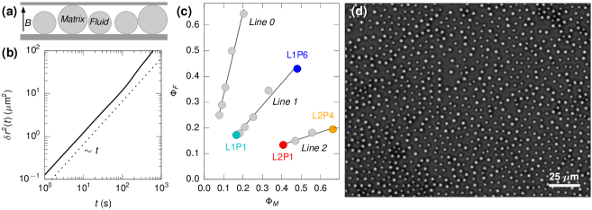
Figure 1: a) Schematic of the experiment, a binary system of small and large particles confined between two glass slides (particle diameters to scale). The large particles support the top slide. The magnetic field $B$ tunes the effective interaction between the particles. b) Snapshot of the system at state point L1P6 in a quadrant of size $214\times 171\upmu$m. c) State diagram for the effective area fractions of the fluid ($\phi_{F}$) versus the matrix particles ($\phi_{M}$). d) Mean-squared displacement for the fluid particles in a very dilute 2D cell. A dashed line indicating diffusive behavior, $\delta r^{2}(t)\sim t$, is shown as a guide to the eye.

II Colloidal model system

The experimental system, as first introduced in Skinner et al. (2013), consist of a binary mixture of super-paramagnetic polystyrene spheres (Microparticles GmbH) of diameters $\sigma_{F}^{0}=3.9~{}\upmu$m (index $F$ for fluid) and $\sigma_{M}^{0}=4.95~{}\upmu$m ($M$ for matrix), respectively, dispersed in water. The particles contain carboxyl surface groups that dissociate in water creating a short-range screened Coulombic repulsion. Their super-paramagnetic properties stem from the iron oxide nanoparticles distributed throughout their polymer matrix and a magnetic dipole will be induced parallel to an externally applied magnetic field.

The binary colloidal suspension is confined between two glass slides to make a 2D sample cell. The large particles act as spacers to support the upper slide and form a fixed matrix, leaving the small particles — the fluid — free to move between them Carbajal-Tinoco et al. (1997); Cruz de León et al. (1998); Santana-Solano and Arauz-Lara (2001); Santana-Solano et al. (2005), see Fig. 1(a). To ensure that the small particles always stay in the plane, the height of the 2D sample cell, $h$, must be less than $h\approx 1.447\sigma_{F}^{0}$ Osterman et al. (2007). The size ratio of the small to the large particles used in the binary mixture is selected accordingly and equals $0.787$. For the preparation of the sample cell, the lower and upper glass slides (Sail $76\times 25\times 1.2~{}$mm and Menzel-Glaser 15 mm $\times$ 15 mm $\times$ 0.15 mm, respectively) are rinsed in distilled water, twice with absolute ethanol and then dried with an air gun. $1.11~{}\upmu$l of the required concentration of colloidal suspension is placed in the centre of the large glass slide to create a $15$ mm $\times 15$ mm $\times 4.95~{}\upmu$m internal sample volume. The small glass slide is placed on top of the solution and a $10~{}$g weight pressure is applied to aid the liquid spread to the edges of the top slide. The edges of the sample cell are sealed with glue (Norland no. 82) and cured under a UV lamp. The cells typically last for 2 days before starting to dry out.

After cell manufacture, the system is equilibrated for 30 minutes. The external magnetic field is set to the required value and the sample allowed to equilibrate for a further 20 minutes. Using optical video microscopy stacks of 8-bit $1280\times 1024$ pixel images of an area of size $428~{}\upmu$m $\times 342~{}\upmu$m are taken at typically 1 Hz for one hour. The colloidal particles are located by standard particle tracking routines Crocker and Grier (1996). An optical microscopy image of the system is shown in Fig. 1(b). The colloids are fairly monodisperse, each with a coefficient of variation of $<3\%$, but this still leads to particles with sizes between the two. This slight size dispersity is noticeable from observation of the colloidal particles in the microscope image, Fig. 1(b). Due to the size dispersity, sometimes fluid particles get stuck and matrix particles stay mobile. So particles are reclassified as fluid or matrix according to their mobility where required. This concerns only a very small fraction of the particles. Any drift in the colloidal particle positions in the microscope are corrected for with respect to the center of mass of the fixed 4.95 $\upmu$m particles. To improve statistics, each image is divided into quadrants. Each quadrant is analyzed separately and mapped onto the hard sphere state diagram. These data points are then binned according to their position on the state diagram to create points averaged over several similar matrix configurations and fluid particle densities.

The repulsive pair potential, $U_{F,M}(r)$, of the super-paramagnetic colloidal particles is controlled via an external magnetic field $B$:

$$U_{F,M}(r)=\mu_{0}\chi_{F,M}^{2}B^{2}/(4\pi r^{3}),$$

where $r$ is the distance between two particles, $\mu_{0}$ is the permeability of free space and $\chi_{F,M}$ the magnetic susceptibility of the fluid or matrix particles. For determining the effective packing fractions of the colloidal particles, effective hard sphere particle diameters $\sigma_{F,M}$ are calculated using the Barker-Henderson approach, Barker and Henderson (1967); Henderson (1977); Hansen and McDonald (2006)

$$\sigma_{F,M}=\sigma_{F,M}^{0}+\int_{\sigma_{F,M}^{0}}^{\infty}~{}(1-e^{-\beta U_{F,M}(r)})dr,$$

where $\sigma_{F,M}^{0}$ are the hard sphere diameters of the colloids and $\beta=1/k_{B}T$. If the magnetic field is switched off, $B=0$, $\sigma_{F,M}$ reduces to the diameter of the colloids $\sigma_{F,M}^{0}$, which corresponds to the lowest state point along each line. Hence, manipulation of both the number densities $n_{F}$ and $n_{M}$ of the colloidal particles, and the effective hard sphere diameters via the external magnetic fields allows different regions of the state diagram to be explored, see Fig. 1(c). We prepared three different samples with different number densities for the matrix and fluid particles, and thus investigated the system along three lines, labelled as lines 0, 1, and 2 in the state diagram. The $n$-th state point of line $x$ is labelled as “L$x$P$n$”. At the lowest point along each line the external field is not yet switched on and thus it is given by the hard sphere area fractions of the matrix $\Phi_{M}^{0}$ and the fluid particles $\Phi_{F}^{0}$. By switching on and increasing the magnetic field the effective area fractions are increased. The size ratio of the fluid to the matrix diameter stays constant at $0.787$, yielding linear paths in the state diagram.

The strength of this experiment lies in the fact that we are able to control the effective area fractions of the colloids without changing the matrix configuration. In this way, we can efficiently measure the tracer dynamics at a range of different effective matrix and fluid area fractions in the same sample. This approach allows us to achieve high matrix area fractions where the matrix still has a random character, a crucial property for a model system for random media. In our analysis of the tracer dynamics, we will focus on the state points along lines 1 and 2. The experimental data are averaged over up to four independent matrix configurations by imaging different parts of each sample.

In order to make sure that the dynamics of the colloids under confinement are well controlled, we prepared a system at a very low matrix packing fraction, with just enough particles to act as spacers, and containing a very low fluid particle concentration. With the 2D trajectory of any tracer particle designated as $\vec{r}(t)$, its mean-squared displacement (MSD) is defined by $\delta r^{2}(t):=\langle(r(t)-r(0))^{2}\rangle$, with $\left<\right>$ representing an average over different matrix configurations, i.e. multiple quadrants, employing multiple time origins, and averaging over all mobile particles. At such low packing fractions, the MSD is expected to exhibit diffusion over all times, $\delta r^{2}(t)\sim D_{0}t$, with $D_{0}$ being the self-diffusion coefficient at infinite dilution, which is confirmed in Fig. 1(d). This indicates that the fluid particles are completely free to diffuse within the 2D cells. Note that diffusion is well-defined in 2D systems with obstacles Bauer et al. (2010).

III Simulation

In order to interpret the experiment, a molecular dynamics (MD) simulation of a comparable two-dimensional system was performed. Note that we are aiming to reveal qualitative and generic features of the localization dynamics across two quite different systems, rather than achieving quantitative agreement between experiment and simulation.

The fixed matrix in the simulation is generated from snapshots of an equilibrated polydisperse liquid of disks interacting with the Weeks-Chandler-Andersen potential Weeks et al. (1971). The pair potential between particles is given by

$$V_{\alpha\beta}(r)=\begin{cases}4\varepsilon_{\alpha\beta}\left[\left(\left(\frac{\sigma_{\alpha\beta}}{r}\right)^{12}-\left(\frac{\sigma_{\alpha\beta}}{r}\right)^{6}\right)+\frac{1}{4}\right],&r<r_{\mathrm{cut}},\\ 0,&r\geq r_{\mathrm{cut}},\end{cases}$$ (1)

with a cutoff of $r_{\mathrm{cut}}=2^{1/6}\sigma_{\alpha\beta}$. The diameters of the matrix particles are sampled from an interval in order to avoid crystallization. The diameters of the $N$ particles are additive, i.e. $\sigma_{\alpha\beta}=(\sigma_{\alpha}+\sigma_{\beta})/2$, with $\sigma_{\alpha}=(0.85+0.3\alpha/N)\sigma_{M}$ and $\alpha,\beta=1,\ldots,N$. The unit of length is thus given by $\sigma_{M}$. The unit of energy is given by the energy scale for the matrix-matrix interaction $\varepsilon_{MM}$. The numerical stability of the simulation is considerably improved by making the potential continuous at the cutoff. This is achieved by multiplying $V_{\alpha\beta}(r)$ with a smoothing function $\Psi(r):=(r-r_{\mathrm{cut}})^{4}/[h^{4}+(r-r_{\mathrm{cut}})^{4}]$ with width $h=0.005\,\sigma_{M}$. As a consequence, we do not observe any problems with energy drift in microcanonical simulations. The particles are equilibrated with a simplified Andersen thermostat Andersen (1980) at temperature $k_{B}T=\varepsilon_{MM}$, where the particle velocities are randomly drawn every 100 time steps from the Maxwell distribution with thermal velocity $\text{v}_{\mathrm{th}}:=(k_{B}T/m)^{1/2}$. The unit of time is thus given by the Lennard-Jones time $t_{0}:=\sigma_{M}/\text{v}_{\mathrm{th}}=[m(\sigma_{M})^{2}/\varepsilon_{M}]^{1/2}$. We integrate Newton’s equations of motion for the particles with the velocity-Verlet algorithm Binder et al. (2004) using a numerical timestep of $\Delta t=7.2\cdot 10^{-4}t_{0}$.

We considered square-shaped systems containing $N=500$, $1000$, $2000$, $4000$, and $16000$ particles, and employed periodic boundary conditions. To allow for sufficient averaging over different matrix configurations, we generated 100 statistically independent configurations for each case. These were equilibrated at the number density $n=N/L^{2}=0.278/\sigma_{M}^{2}$, were fixed and subsequently uniformly rescaled to number density $n=0.625/\sigma_{M}^{2}$, and thus correspond to the system sizes $L/\sigma_{M}=28.28$, $40$, $80$, and $160$. Varying the system size $L$ allows us keep finite size effects under control.

Into the matrix structures, we insert a gas of tracer particles which do not interact with each other. The interaction of the tracers with the matrix is given by the WCA potential of Eq. 1 with parameters $\varepsilon_{\alpha\beta}=0.1\varepsilon_{M}$ and $\sigma_{\alpha\beta}=(\sigma_{M}+\sigma_{F})/2$. Note that the polydispersity of the matrix particles is neglected here, as it was only used to avoid crystallization of the matrix configurations. The diameter $\sigma_{F}$ of the tracer particles acts as the control parameter and is used to change the area inaccessible to the tracer particles without changing the matrix structure, equivalently to modifying the magnetic field in the experiment.

The tracer particles are inserted and equilibrated also with the simplified Andersen thermostat. Since the particles are non-interacting, the equilibration times can be quite short with run times of typically $10^{3}t_{0}$. For the microcanonical production runs we considered two cases. In the one case — the confined ideal gas — the production run is carried out directly after the equilibration, and the particles naturally have a broad distribution of energies. But the systems are first brought to the same average energy by rescaling all tracer velocities in each system with one constant, leaving the relative distribution of energies unmodified. In the other case — the single-energy case — we enforce that all tracers have exactly the same energy. This is achieved by determining the average tracer energy at the end of the equilibration run, and reinserting the particles at random places, provided that their potential energy at that position is lower than the average energy and assigning the rest of the energy as kinetic energy. After that, microcanonical simulation runs are started for both cases with run times of up to about $2\cdot 10^{5}t_{0}$. The single-energy case was shown to exhibit the universal critical behavior of the Lorentz gas with the transition occurring at the critical diameter $\sigma_{F}^{\mathrm{c}}\approx 0.43$, while the confined-ideal-gas case shows strong rounding Skinner et al. (2013); Schnyder et al. (2015).

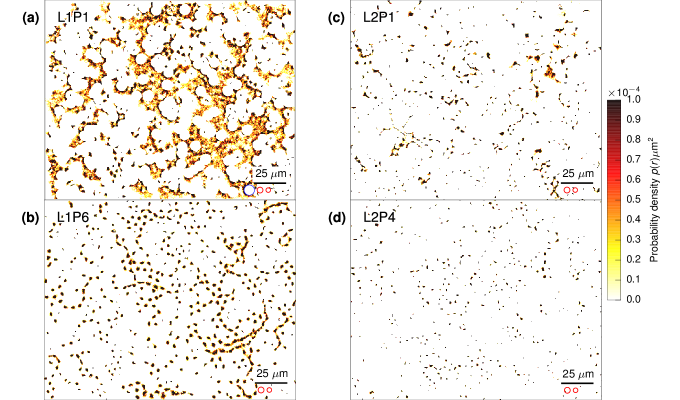
Figure 2: Experiment: Single-particle probability distributions from 2D histograms of all colloidal particle positions in a quadrant measured over the duration of an hour for state points (a) L1P1, (b) L1P6, (c) L2P1, and (d) L2P6. Normalized such that the total probability of the whole quadrant is $1$. Size of the colloids annotated as red circles under the scales at the bottom right of each plot, size of the hard-core excluded area for centers of mobile particles indicated in (a) as blue circle under the scale.

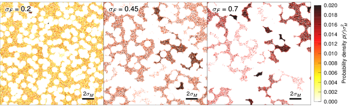
Figure 3: Simulation: Single-particle probability distributions from 2D histograms in the confined ideal gas case. Shown are square sections of length $20\sigma_{M}$ and the histograms are normalized such that the total probability integrated over the shown section is $1$.

IV Results and discussion

In our previous work Skinner et al. (2013), we used MD simulations to demonstrate that the experiment exhibits a delocalization-localization transition similar to the Lorentz gas, but that in contrast to the latter, the transition is rounded due to the soft interactions between the particles. Here, we revisit the experiment and the simulations, and analyse the structure of both the matrix and mobile component, as well as investigate the strongly heterogenous single-particle dynamics. With our analysis of the intermediate scattering function we get additional insights into the rounding of the localization transition, expanding on and complementing our previous work. As line 0 is very similar to line 1, it will be left out of the discussion.

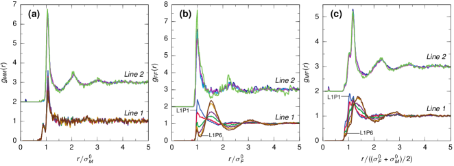
Figure 4: Experiment: Partial radial distribution functions, for the (a) matrix-matrix interaction $g_{MM}(r)$, (b) fluid-fluid interaction $g_{FF}(r)$, and (c) fluid-matrix interaction $g_{FF}(r)$ for each state point along lines 1 and line 2. Line 2 is shifted by 2 in each plot.

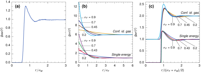
Figure 5: Simulation: Partial radial distribution functions, for the (a) matrix-matrix interaction $g_{MM}(r)$, (b) fluid-fluid interaction $g_{FF}(r)$, and the fluid-matrix interaction $g_{FF}(r)$ for the single-energy and confined-ideal-gas cases (the latter data is shifted upwards by 5 in (b) and by 1 in (c)).

IV.1 Histograms

Because we are able to track the full trajectories of the colloidal particles, we can directly calculate the probability density $p(\vec{r})$ of finding a single particle at position $\vec{r}$. To this end, we compute the histogram of all positions of the particle centers over the duration of the experiment (1h) on a grid where each bin corresponds to one pixel on the camera sensor, i.e. $\Delta A=(0.34\upmu\text{m})^{2}$, and normalizing the distribution such that the integral over a whole quadrant is unity. The distributions, shown in Fig. 2, give a good qualitative feel for the structure of the available free area and the dynamics of the tracer particles in the system and how it is modified when crossing the localization transition in the system. The obstacles are clearly visible as circular areas to which the fluid particles are excluded. At L1P1, where the magnetic field is switched off, the quadrant shown in Fig. 2(a) clearly shows a percolating path from the top center to the bottom right. At high magnetic fields, the motion of the fluid particles becomes severely constrained, see L1P6 in Fig. 2(b) where the same quadrant as in (a) is shown. The particles explore their surroundings, but on the time scales available to the experiment travel not much farther than their own diameter. This is not only due to the constriction of the matrix but also due to competition for free space between the mobile particles. However, the areas explored by the tracers are still connected in many cases, and large clusters of connected free area are found in the whole quadrant. It is probable that there is no percolating path present in the system and thus the sample is likely localized. Still, the MSD in this system becomes diffusive at long times Skinner et al. (2013), which is an indicator for the rounding of the localization transition. The systems along line 2 are all strongly localized, regardless of the strength of the magnetic field, see Fig. 2 (c,d).

For qualitative comparison, we calculated analogous histograms for the simulation of the confined ideal gas, see Fig. 3. The length scales are comparable, i.e. the obstacles are depicted at comparable size. At very small diameters, e.g. $\sigma_{F}=0.2$ in Fig. 3, the available area is highly connected, a situation that is not encountered in the experiment. The histogram at $\sigma_{F}=0.45$ in Fig. 3 represents the situation close to the percolation point, where clusters of free area still span nearly the whole system. This is qualitatively comparable to the situation of L1P1 and L1P6. Highly dense systems contain only clusters of a linear extent of a few particle diameters, see $\sigma_{F}=0.7$ in Fig. 3. This situation is comparable to L2P1 and L2P4. While in certain ways the experiments and simulations are comparable, it is clear that it is extremely difficult to perform the experiments for long enough as to allow for the particles to sample the full available free area close to the critical point, a limitation that the simulations do not have.

IV.2 Matrix and fluid structure

In Ref. 20, we characterized the structure of the matrix via the static structure factor and demonstrated that the matrix remains unchanged along each line, even at large magnetic fields $B$. It is revealing to also study the structure of the fluid, and as we have access to the trajectories of the particles in the sample, we can fully quantify the structural correlations in the system by calculating the partial radial distribution functions, $g_{\alpha\beta}(r)$ Hansen and McDonald (2006),

$$g_{\alpha\beta}(r)=\frac{A}{2\pi r}\frac{1}{f_{\alpha\beta}}\left\langle\sum_{i=1}^{N_{\alpha}}\sum_{j=1,\neq i}^{N_{\beta}}\delta(r-|\vec{r_{j}}-\vec{r_{i}}|)\right\rangle,$$ (2)

$$\text{with}\quad f_{\alpha\beta}=\begin{cases}N_{\alpha}(N_{\alpha}-1)&\text{ for }\alpha=\beta,\\ N_{\alpha}N_{\beta}&\text{ for }\alpha\neq\beta.\end{cases}$$

Here, $\alpha,\beta\in[F,M]$, $N_{\alpha}$ is the number of particles in component $\alpha$, $\vec{r}_{i}$ and $\vec{r}_{j}$ are the positions of particles $i$ and $j$ of components $\alpha$ and $\beta$, and $A$ is the area of the system or quadrant that is being evaluated.

In the experiment, the matrix-matrix component of the radial distribution function, $g_{MM}(r)$, for line 1, see Fig. 4(a), only exhibits a maximum for particles at contact, demonstrating that the matrix particles are nearly spatially uncorrelated. We observe a small pre-peak at $r\approx 0.9\sigma_{M}^{0}$ which probably comes from small particles getting stuck and thus being identified as fixed particles. The smallness of this peak demonstrates that this is only a very small effect. The function stays unchanged as the magnetic field is modified, demonstrating that the matrix particles really are fixed. In contrast, the fluid structure as characterized by $g_{FF}(r)$ is strongly modified by the presence of the magnetic field, see Fig. 4(b). At zero magnetic field at L1P1 many particles are in contact, as demonstrated by the single maximum of $g_{FF}(r)$ at $r=\sigma_{F}^{0}$. With increasing magnetic field, the particles are driven further apart and the maximum decreases in amplitude. At the same time, another maximum appears and gradually shifts to larger $r$, in agreement with the growth of the effective diameter of the particles. Also, multiple smaller minima and maxima develop, indicating that the particles become more structurally correlated. At L1P6 a small peak remains at the original position of the maximum ($\sigma_{F}^{0}$), which indicates the a small portion of fluid particles cannot move away from each other even though the repulsive interaction is quite strong. The matrix-fluid radial distribution function $g_{MF}(r)$ behaves quite similarly to $g_{FF}(r)$.

Line 2 differs from line 1 by having considerably larger number densities for both fluid and matrix particles. Consequently, the spatial correlations frozen in the matrix are stronger in line 2 as compared to line 1 and lead to a series of maxima and minima beside the main maximum of particles being at contact, see Fig. 4(a). Still, the matrix is fairly disordered with the extrema not being very pronounced. As for line 1, $g_{MM}(r)$ is independent of the magnetic field. In contrast to line 1, the fluid pair correlation function $g_{{}_{FF}}(r)$ is unchanged by the magnetic field, as well. This indicates that the particles are already so strongly confined by the matrix that increasing the repulsion between particles does not change their relative positions. The maximum of $g_{FF}(r)$ is very near the hard-sphere diameter of the particles, indicating that many fluid particles are at contact, fully occupying the free area inside the matrix and not leaving room to move around. Finally, similar to line 1, the matrix-fluid radial distribution function $g_{MF}(r)$ behaves quite similarly to $g_{FF}(r)$.

The data demonstrates the level of control we have over the structure of the system in the experiment. By varying the magnetic field, we can strongly influence the structure of the fluid, at least in the case of line 1 where the matrix density is moderate. The ability to calculate the partial pair correlation functions from the full trajectories of the colloidal particles demonstrates the strength of the colloidal model experiment, as the same would be very difficult to achieve in atomic systems or in analogous 3D colloidal systems with tuneable interactions.

In the simulation, the chosen matrix structure, see Fig. 5(a), is roughly comparable to the one found along line 1 in the experiment (Fig. 4(a)). Both are gas-like in structure with the experiment having a sharper peak. The main difference of the simulation to the experiment is that the simulated tracer particles do not interact with each other. This leads to considerably different structural correlations in the fluid, see Fig. 5(b). In contrast to the experiments, see Fig. 4(b), the particles are allowed to overlap, as indicated by the maximum of $g_{FF}(r)$ at $r=0$. As the particles become bigger, available space becomes increasingly rare, and the probability of tracers overlapping grows. Notably, the single-energy and confined-ideal-gas cases show very similar structural correlations. The matrix-fluid particle pair correlation function $g_{MF}(r)$ is also similar for both cases, see Fig. 5(c). The function exhibits a maximum at $r=(\sigma_{M}+\sigma_{F})/2$, indicating that many tracers are at contact with matrix particles. The maximum of $g_{MF}$ in the confined ideal gas exhibits a less steep left shoulder due to the broad distribution of effective diameters in the system. As the size of the tracers increases, that maximum becomes sharper but stays at the same position. This is different from line 1 in the experiment and is again a result of the lack of interaction between the tracers.

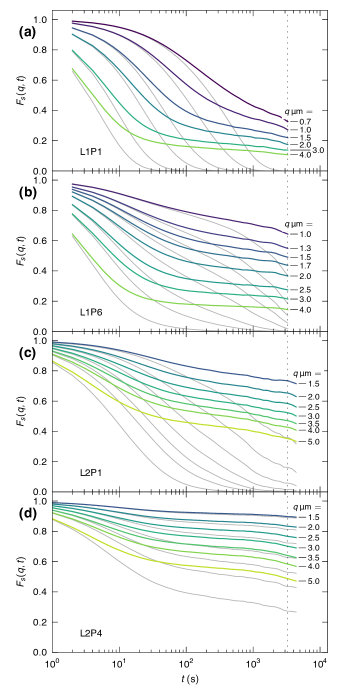
Figure 6: Experiment: Self part of the intermediate scattering function $F_{\mathrm{s}}(q,t)$ for the fluid particles for a range of wave numbers $q$ relating to state points (a) L1P1, (b) L1P6, (c) L2P1, and (d) L2P6 (in colors), as well as the corresponding Gaussian approximations (in grey). A measure of the non-ergodicity parameter is obtained with $f_{\mathrm{s}}(q)\approx F_{\mathrm{s}}(q,t\approx 3300s)$, indicated by the dotted line, and shown in Fig. 8.

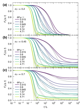
Figure 7: Simulation: Self part of the intermediate scattering functions in the simulation for the single-energy case (colored dashed lines) and the confined ideal gas case (colored solid lines) for particle diameters (a) $\sigma_{F}=0.2$, (b) $0.45$, (c) $0.7$, as well as the corresponding Gaussian approximations (in grey).

IV.3 Dynamics

IV.3.1 Self-intermediate scattering function

The self-part of the intermediate scattering function (SISF) for the mobile particles is defined as

$$F_{s}(q,t)=\frac{1}{N_{F}}\left\langle\sum_{j=1}^{N_{F}}\exp\{i\vec{q}\cdot[\vec{r_{j}}(t)-\vec{r_{j}}(0)]\}\right\rangle,$$ (3)

with the 2D wave vector $\vec{q}$. Since the system is statistically isotropic, the SISF is invariant under the rotation of the direction of the wave vector and only depends on its magnitude, the wave number $q:=|\vec{q}|$. The SISF gives the full probabilistic information in Markovian systems and can be directly measured in scattering experiments. The SISF at any given $q$ describes the relaxation of density fluctuations on length scales $1/q$ over time. Its long-time limit $f_{\mathrm{s}}(q):=\lim_{t\to\infty}F_{\mathrm{s}}(q,t)$ is known as the non-ergodicity parameter or the Lamb-Mößbauer factor, and is a measure of the fraction of particles that are localized on a length scale $1/q$. Even though the self-part of the van Hove function discussed in Ref. Skinner et al. (2013) contains the same information, it is of merit to study the SISF as well, since it is more sensitive to localized particles than both the van Hove function and its second moment, the mean-squared displacement, $\delta r^{2}(t)$, which are more sensitive to highly mobile particles.

In the experiment, the SISF can be computed directly from the particle trajectories using Eq. (3) and we observe from Fig. 6 that the SISF approximately has the same shape for all measured state points. The SISF decays in a single relaxation step onto a finite long-time limit $f_{\mathrm{s}}(q)$, which increases with density, i.e. L1P1 $\rightarrow$ L1P6 and L2P1 $\rightarrow$ L2P4, and with larger length scales, i.e. smaller $q$. Note that this is qualitatively different from the two-step relaxation found in ideal glass formers Van Megen and Underwood (1993); Götze (2009). Even at the low densities of L1P1, fluid particles are trapped in voids created by the matrix, rendering the dynamics non-ergodic and preventing the SISF from decaying fully. For comparison, the SISF of the simulations are shown in Fig. 7. Qualitatively, the single-energy and the confined ideal gas cases are extremely similar to each other. There is a single relaxation step onto a finite plateau which increases with increasing density, i.e. increasing $\sigma_{F}$, and larger length scales, i.e. smaller $q$. The main difference between the single-energy and confined ideal gas cases can be found in the short-time behavior around $t/t_{0}=\mathcal{O}\left(1\right)$, where the single-energy case resolves the first collision of the tracers, while this is averaged out in the confined-ideal-gas case. Apart from that, only the magnitude of the long-time limits is different in the two cases. In extremely dilute systems, e. g. $\sigma_{F}=0.2$, the long-time limit is nearly 0, indicating that only a small fraction of particles is localized. At larger diameters, e. g. $\sigma_{F}=0.45$ and $0.7$ in Fig. 7 (b, c), the long-time limits are finite, and the SISF of experiment and the confined-ideal-gas case in the simulation become qualitatively very similar.

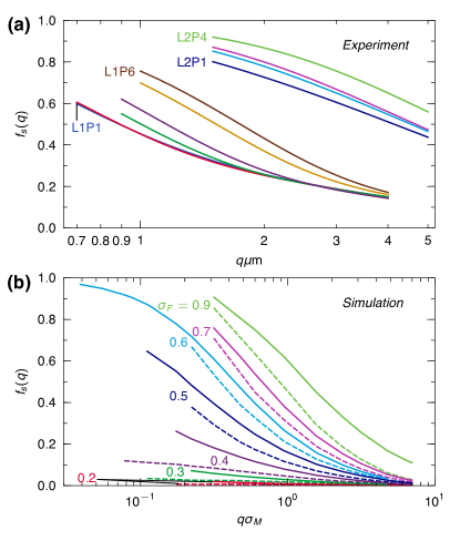
Figure 8: (a) Long-time limit of the SISF $f_{\mathrm{s}}(q)$ of the experiment along lines 1 and 2 in semilogarithmic presentation. (b) Long-time limit of the SISF $f_{\mathrm{s}}(q)$ in the simulation for the single-energy (dashed) and ideal-gas case (solid).

To quantify the proportion of localized particles in the experiment, we approximately determined $f_{\mathrm{s}}(q)$ as the value of $F_{s}(q,t)$ at $t\approx 3300\,\text{s}$ (indicated by the vertical dashed lines in Fig. 7) for all points along both line 1 and 2, see Fig. 8 (a). Note that this simply corresponds to the longest accessible timescale in the experimental data. The $f_{\mathrm{s}}(q)$ for the simulations, shown in Fig. 8 (b), are easy to obtain as the simulations have shorter relaxation time scales. Qualitatively, the $f_{\mathrm{s}}(q)$ of the experiment and simulations exhibit similar dependence on $q$. The $f_{\mathrm{s}}(q)$ of line 1 of the experiment is similar to the $f_{\mathrm{s}}(q)$ of the simulation for small $\sigma_{F}$ and the $f_{\mathrm{s}}(q)$ of line 2 corresponds to that of the simulations at large $\sigma_{F}$. In all experimental state points $f_{\mathrm{s}}(q)$ is finite, showing that even at the lowest densities along each line there are subsets of particles that are localized, similarly to the Lorentz model. Importantly, the SISF and $f_{\mathrm{s}}(q)$ of both experiment and simulation look qualitatively the same on both sides of the transition.

From the simulations we can further conclude that the dynamics is more heterogeneous in the confined ideal gas than in the single energy case, i.e. the Lorentz gas. This is inferred from the fact that the $f_{\mathrm{s}}(q)$ at the same $\sigma_{F}$ is larger in the confined ideal gas case, indicating a larger fraction of particles is localized, while, at the same time, the MSD of the confined ideal gas grows faster at long times that that of the single energy case (see Fig. 2b in Ref. 20), indicative of more highly mobile particles. This increase in heterogeneous dynamics in the confined ideal gas case as compared to the single energy case is a trivial consequence of the broad energy distribution of the particles.

IV.3.2 The Gaussian approximation

Next, we analyse the cumulants of the SISF, since this exposes dynamical heterogeneities more clearly. The SISF can be expressed via a cumulant expansion for small wave numbers as Höfling and Franosch (2013)

$$F_{s}(q,t)=\exp\left[-\frac{q^{2}\delta r^{2}(t)}{4}+\frac{1}{2}\alpha_{2}(t)\left(\frac{q^{2}\delta r^{2}(t)}{4}\right)^{2}+...\right],$$

with the non-Gaussian parameter (NGP), $\alpha_{2}(t)$, relating the MSD, $\delta r^{2}(t)$, and the mean-quartic displacement (MQD), $\delta r^{4}(t)$, to each other Rahman (1964):

$$\alpha_{2}(t):=\frac{1}{2}\ \frac{\delta r^{4}(t)}{[\delta r^{2}(t)]^{2}}-1.$$

The cumulants $\delta r^{n}(t)$ are defined as

$$\delta r^{n}(t):={\left\langle\vphantom{1^{2}}|r(t)-r(0)|^{n}\right\rangle}=\int|r|^{n}P(r,t)\ \text{d}^{d}r,$$ (4)

with the self-van-Hove function $P(r,t)$ being the one-particle density autocorrelation function in space and time, and the inverse Fourier transform of the SISF,

$$P(r,t):=\frac{1}{N_{F}}{\left\langle\vphantom{1^{2}}\sum_{j=1}^{N_{F}}\delta\left[r-\left|\vec{r}(t)-\vec{r}(0)\right|\right]\right\rangle}.$$

The odd-numbered cumulants vanish due to the rotational symmetry of the system.

If the system exhibits diffusion, the SISF is Gaussian at all times and can be directly related to the MSD as follows

$$F_{\mathrm{s}}(q,t)=\exp\left(-\frac{q^{2}\delta r^{2}(t)}{4}\right),$$ (5)

which is known as the Gaussian approximation Hansen and McDonald (2006). This approximation is valid for many systems, e.g. for the diffusive motion of hard spheres Thorneywork et al. (2016), or for harmonic oscillators Vineyard (1958), and $\alpha_{2}(t)$ is either exactly or close to 0 in these cases. The failure of the Gaussian approximation indicates, for instance, the presence of correlated motion, localization of particles on many different length scales, or the presence of multiple relaxation times, and is a strong indication of dynamical heterogeneity in the system Kob et al. (1997); Yamamoto and Onuki (1998); Weeks et al. (2000), which is often quantified using the NGP. In the Lorentz model the Gaussian approximation fails as well Lowe et al. (1997), in particular at the critical point and $\alpha_{2}(t)$ never decays to 0, but instead exhibits a divergence Spanner et al. (2011). This is a result of the particles being confined in a fractal structure and leads to its extended subdiffusion.

We find that the Gaussian approximation provides a good description of the SISF of all experimental and simulation data at short times, see Figs. 6 and 7. At long times it typically fails to capture the long relaxation times and the plateau heights. If the system becomes extremely localized, however, the Gaussian approximation matches the SISF more closely again, as illustrated in Fig. 6(d) for the experimental data at L2P4. Here, the particles mostly vibrate in small cages created by both matrix and neighboring fluid particles and the dynamics then effectively approaches the idealization of localization in harmonic potentials. As a consequence, the Gaussian approximation is found to be least successful close to the localization transition, as expected for the Lorentz model.

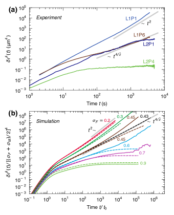
Figure 9: Mean-quartic displacement $\delta r^{4}(t)$ for experiment (a) and simulation (b) as a function of time. In the simulation, single-energy case (dashed lines) and confined-ideal-gas case (solid lines) are shown. The straight grey lines $\sim t^{2}$ and $\sim t^{4/\hat{z}}$ with $\hat{z}\approx 2.955$ serve as guide to the eye.

IV.3.3 The mean quartic displacement

In the Lorentz model the mean-quartic displacement is expected to grow as $\delta r^{4}(t)\sim t^{2}$ at long times in the delocalized state, corresponding to regular diffusion, and becomes constant in the localized state. Close to the transition, it is expected to grow as $\delta r^{4}(t)\sim t^{4/\tilde{z}}$ with exponent $\tilde{z}\approx 2.955$ in two dimensions Höfling et al. (2006). The experimental data exhibit a transition from delocalized dynamics at L1P1 to localized dynamics at L2P4, with subdiffusive growth of the MQD at L1P6 and L2P1. The growth of the MQD at L1P6 at large times seems very loosely compatible with the Lorentz-model power law at the transition, but at closer inspection has a lower effective exponent. The simulation in the single-energy case is in full agreement with the Lorentz-model scenario, see Fig. 9(b), making the transition from delocalized to localized dynamics and exhibiting extended power-law growth at the critical point at $\sigma_{F}=0.43$ with the expected exponent. This shows once more that the single-energy case falls in the same universality class as the Lorentz model. The MQD for confined ideal gas shows strong rounding similar to the MSD Skinner et al. (2013): the MQD exhibits the transition from delocalized to localized behavior but the transition is smoothed due to the averaging over a wide range of particle energies, which results in a wide range of effective exponents rather than the critical asymptote. Strikingly, at $\sigma_{F}=0.6$, the MQD of the confined ideal gas initially follows the corresponding curve of the single-energy case, indicating localization of most particles, but at long times becomes dominated by the contributions of a few highly mobile, delocalized particles. This leads to subdiffusion over many orders of magnitude in time with an effective exponent smaller than the critical one – similar to what is observed for the MQD in the experiment at L1P6 – before crossing over to $\sim t^{2}$ at long times in the simulation. Note that we do not reach this time scale in the experiment. All of this is characteristic of the rounding of the localization transition.

Figure 10: Non-Gaussian parameter for the experiment (a), and for the simulation in the (b) single-energy and (c) confined-ideal-gas cases.

IV.3.4 The non-Gaussian paramater

The non-Gaussian parameter (NGP), $\alpha_{2}(t)$, is very sensitive to dynamical heterogeneities Kegel and van Blaaderen (2000); Shell et al. (2005). In the experiment, the NGP on the delocalized side of the transition, i.e. along line 1, grows from nearly zero, characteristic of regular diffusion at short time scales, to values around 2 at long times for both state points L1P1 and L1P6, see Fig. 10 (a). On the timescale of the experiment, these NGPs do not decay, clearly showing that the dynamics remains non-Gaussian and heterogeneous. Note that this is qualitatively different from typical glassy dynamics, where the NGP goes through a maximum at intermediate times and decays to zero at long times Kim et al. (2011). Along line 2 of the experiment, i.e. on the localized side of the transition, the NGP is already close to unity at early times for both L2P1 and L2P4. While L2P4 remains relatively constant but finite, the NGP for L2P1 – which is close to the localization transition – grows strongly with time.

To interpret the behaviour of the NGP in the experiment, we now discuss the NGP in the simulation. First we consider the single energy case, which reproduces the Lorentz model Höfling et al. (2006); Höfling and Franosch (2007); Höfling et al. (2008); Spanner et al. (2011). In this case, the NGP parameter exhibits critical divergence at the localization transition, $\sigma_{F}=0.43$, see Fig. 10 (b). Indeed, the exponent is nearly indistinguishable from the expected critical exponent of $\approx 0.0361$ in two dimensions Höfling et al. (2006). The small deviation from the asymptote at long times is most likely due to lacking statistics although we cannot fully rule out small finite size effects, which have been shown to particularly affect the NGP Spanner et al. (2011). However, the experiment and the single energy case clearly exhibit very different behavior and the critical divergence of the Lorentz model is so small that it cannot explain the experimental data.

Therefore, we now consider the NGP of the confined ideal gas, which is shown in Fig. 10 (c). In this case, the NGP grows monotonically to long time values that are generally larger than those found in the single-energy case (note the different scales of the axes). Close to the rounded localization transition, $0.45\leq\sigma_{F}\leq 0.7$, the NGP exhibits very strong growth, far exceeding those of the single-energy case. Strikingly, the confined ideal gas shows qualitatively similar behavior to the experiment, while being very different from the Lorentz model scenario seen in the single energy case. Importantly, this indicates that the observed heterogeneous and non-Gaussian dynamics in the experiment are not due to critical dynamics, but are a direct result of the rounding of the localization transition. In other words, the divergence of the NGP in the confined ideal gas is different from the weak critical divergence of the NGP in the Lorentz model. Because the NGP is not very sensitive to the critical dynamics, it exposes the non-Gaussian dynamics that occurs in the experiment and the confined ideal gas due to the rounding of the localization transition.

V Conclusion

We have studied the dynamics of a quasi-two-dimensional colloidal fluid confined in a strongly heterogeneous matrix. The experiment exhibits a rounded localization-delocalization transition, in which the critical point is seemingly avoided. We have shown that the dynamics in the experiment is strongly non-Gaussian and by comparing the experiment to molecular dynamics simulations of a confined ideal gas, we have demonstrated that the heterogeneous and non-Gaussian dynamics are a generic feature of the rounding of the localization transition. In addition, we have characterized the structure of the confining matrix and fluid particles in terms of the partial pair distribution functions.

The anomalous dynamics close to the transition has been analyzed with a particular focus on dynamical heterogeneities, by consideration of the self part of the intermediate scattering function, the mean-quartic displacement, and the non-Gaussian parameter. The self intermediate scattering functions decay in one step to their long-time limit, similar to the Lorentz gas, but different from typical glassy behavior. A large fraction of particles can be already localized while the mean-squared displacements, discussed in Ref. 20, is still diffusive. Although this heterogeneity is typical for the Lorentz gas – which is reproduced in our simulations when all the particles are assigned the same energy – we have found that the heterogeneity is significantly enhanced when this energy constraint is removed and a confined ideal gas is considered. Strikingly, this leads to a strong increase of the non-Gaussian parameter close to the rounded localization transition, as also found in the experiments, which is different from the weak divergence predicted for the Lorentz gas. The comparison between the experiment and the simulations show how the soft interactions make the dynamics more heterogenous compared to the Lorentz gas and lead to strong non-Gaussian fluctuations.