A mathematical model for mechanically-induced deterioration of the binder in lithium-ion electrodes

Abstract

This study is concerned with modeling detrimental deformations of the binder phase within lithium-ion batteries that occur during cell assembly and usage. A two-dimensional poroviscoelastic model for the mechanical behavior of porous electrodes is formulated and posed on a geometry corresponding to a thin rectangular electrode, with a regular square array of microscopic circular electrode particles, stuck to a rigid base formed by the current collector. Deformation is forced both by (i) electrolyte absorption driven binder swelling, and; (ii) cyclic growth and shrinkage of electrode particles as the battery is charged and discharged. In order to deal with the complexity of the geometry the governing equations are upscaled to obtain macroscopic effective-medium equations. A solution to these equations is obtained, in the asymptotic limit that the height of the rectangular electrode is much smaller than its width, that shows the macroscopic deformation is one-dimensional, with growth confined to the vertical direction. The confinement of macroscopic deformations to one dimension is used to obtain boundary conditions on the microscopic problem for the deformations in a ’unit cell’ centered on a single electrode particle. The resulting microscale problem is solved using numerical (finite element) techniques. The two different forcing mechanisms are found to cause distinctly different patterns of deformation within the microstructure. Swelling of the binder induces stresses that tend to lead to binder delamination from the electrode particle surfaces in a direction parallel to the current collector, whilst cycling causes stresses that tend to lead to delamination orthogonal to that caused by swelling. The differences between the cycling-induced damage in both: (i) anodes and cathodes, and; (ii) fast and slow cycling are discussed. Finally, the model predictions are compared to microscopy images of nickel manganese cobalt oxide cathodes and a qualitative agreement is found.

1 Introduction

Much current research is focused on the development of lithium-ion batteries for use in a variety of areas, ranging from consumer electronics to the automotive industry, with the current market for such devices being in excess of $20bn (USD) per annum and set to increase further [29]. Many previous studies have considered how to model the electrochemical processes occurring within such cells, with the aim of informing optimal design. The majority of these studies have been, at least partially, based on the seminal models of Newman et al.[16, 17, 22, 23], which account for the complex battery microstructure using ‘averaged’ quantities—an approach that has been subsequently formalized in [48, 12]. Providing an exhaustive list, or even a summary, of the extant work on lithium-ion batteries is almost impossible and instead we point to the following reviews [38, 61, 3]. Of particular interest is modeling that can inform design improvements in terms of increased energy density, facilitation of higher charge/discharge rates, and improved safety and cycling lifetime. Here, we will focus on the last of these, specifically the (detrimental) morphological changes that can occur during cell fabrication and usage as a result of the development of internal mechanical stresses in response to (i) polymer binder swelling due to electrolyte absorption, and; (ii) dilation (and contraction) of the electrode particles as the cell is cycled.

Lithium-ion batteries comprise four key constituents: (i) the anode (the negative electrode during discharge); (ii) the cathode (the positive electrode during discharge); (iii) the electrolyte, and; (iv) a porous separator that ensures unhindered passage of ionic current (via the electrolyte) while electronically isolating the two electrodes, see Figure 1.1. This assembly is sandwiched between two metallic current collectors (CCs). In commercial cells both the anode and cathode have a complex morphology; both are typically composed of small particles ($\sim$1-10$\mu$m) of active material (AM) embedded in a porous polymer binder matrix which (in the case of the cathode) is doped with highly conducting acetylene black nano-particles. The pores within the polymer matrix (of typical size 10–100nm) form channels through which the electrolyte can penetrate — see Figure 2. The binder performs two key tasks; firstly it ensures the structural integrity of the electrode and secondly it serves to connect electrode particles electronically to the current collector.

Figure 1: A schematic of a coin cell.

After manufacture, when such electrodes are assembled as part of a cell, they are soaked in electrolytic fluid which is absorbed by the binder and results in significant swelling of this polymer phase. Commonly used binders include polyvinylidene fluoride (PVDF) and carboxymethyl cellulose (CMC), and each of these materials is known to exhibit expansions of around $50\%$ by volume ($75\%$ by weight) after begin immersed in EC:DMC for a few hours/days [11, 36, 41]. Even though this binder/acetylene black phase only constitutes a relatively small fraction of the material making up an electrode — typical figures for the AM:filler ratio by weight (here filler denotes both polymer binder and acetylene black) range from 70:30 to 90:10 in cathodes [32, 34] and 90:10 to 95:5 in anodes [5, 60] — a 50% volumetric expansion has the potential to lead to significant deformations and stresses (and ultimately morphological damage to the electrode) [50].

After assembly, when the cell is under operating conditions, the chemical potential difference between the positive and the negative electrodes leads to charge transfer events (redox/(de-)intercalation reactions) in the electrode particles. Importantly, these reactions are accompanied by volumetric changes in the electrode particles. By far the most commonly used active material in commercial anodes is graphitic carbon (LiC₆). On lithiation (associated with battery charging) these anode particles exhibit a significant volumetric expansion, of around 10% [14, 46]. In contrast typical cathode active materials (e.g. cobalt oxide (LiCoO₂), iron phosphate (LiFePO₄) and nickel manganese cobalt oxide (LiNiMnCoO₂)) exhibit smaller, but nonetheless appreciable, volumetric expansions in the range of 2–4% [59, 39]. This swelling/contraction of the active material phase can lead to large mechanical stresses within the electrodes which, in turn, can lead to delamination of the binder from the electrode particles and the CC. Notably delamination, as seen in Figure 2 occurs preferentially (at least early on) in the plane parallel to the current collector and it is one of the goals of this work to explain this pattern of delamination.

In unfavorable cases, structural change within the electrode has detrimental effects on cell performance. For example, delamination of the binder from the surfaces of the electrode particles and CC (as can be seen in Figure 2) has been proposed as a cause of degradation, and has been shown to cause both a measurable decrease in the ‘connectivity’ and the bulk (or ‘effective’) electronic conductivity of cathodes [19, 26, 27, 30, 33, 49, 52]. In addition to decreasing the efficacy of electron conduction, the delamination process can increase current densities (by reducing the area of electronic contact) and in turn enhance Joule heating, an effect which has the potential to cause to thermal runaway [55]. Delamination also exposes additional areas of the surfaces of the electrode particles directly to the electrolyte leading to the formation of extra solid electrolyte interface (SEI) layers [43] and to the consumption of active lithium (from the electrolyte), an effect that results in decreased battery capacity.

Whilst a good deal of work has been focused on: (i) characterizing the mechanical processes occurring within various different types of active material, e.g. phase changes and particle fracturing [44, 9, 10, 63, 57]; (ii) discerning the impact of cycling-induced compression of, and the consequent reduction of pore space in, separator membranes on long-term cell performance [42, 24, 25], and; (iii) understanding the relatinship between the stack pressure, in e.g. commerical pouch cells, and the health of the cells [35, 6, 7]; much less has been done to elucidate the mechanical behavior of individual electrodes (including the binder) as a whole. Previous modeling in this area includes [40, 58]. The former considers the effects of electrode particle expansion and contraction on electrical connectivity when the surrounding matrix is composed entirely of carbon black particles. However, the absence of a binder material means these results are irrelevant to commercial cells. In contrast, whilst [58] does model the binder material, it focuses almost entirely on predicting stresses within the electrode particles. Here we focus primarily on modeling the deformations of the binder itself in response to: (i) its swelling in response to electrolyte absorption, and; (ii) swelling/contraction of the electrode particles as the cell is cycled. We work within an idealized 2-dimensional geometry as illustrated in Figure 3. The electrode is assumed to be initially rectangular, with its bottom surface bound to a rigid current collector, while the electrode particles are taken to be circular cylinders with centers located on a regular square lattice. The mechanical evolution of the electrode is described by a model based on Biot’s theory of poroelasticity [54], but with the additional feature that the porous skeleton is treated as a linear viscoelastic. Closely related models have been proposed previously for studying the behavior and interaction of soil and groundwater in mining applications, see e.g. [1, 4]. Our primary goal here is to use this model to predict the normal stresses, in the binder, on the surfaces of the electrode particles and infer from these whether (and how) delamination occurs.

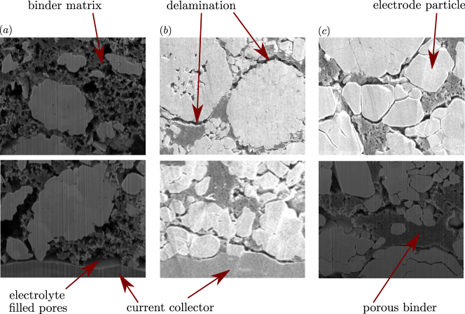
Figure 2: FIB/SEM images of nickel manganese cobalt oxide (NMC) cathodes with a PVDF binder. The lightest material is the NMC active material, the darker material is the polymer binder, the darkest regions are pore spaces which are filled with electrolyte during cell operation, and the (almost) planar material at the bottom of columns (a) and (b) is the aluminum CC. Column (a) shows electrodes that were manufactured in G. Goward’s group (McMaster Chemistry). These images were taken before the electrodes had been immersed in electrolyte, i.e. before they were constructed as part of a cell. Column (b) shows commercial electrodes which have been immersed in electrolyte (1 molar LiPF₆ in EC/DMC), undergone a single ‘formation’ cycle, and then been removed from their housing and allowed to dry. Column (c) also shows commercial electrodes, but these have been immersed in electrolyte (again, 1 molar LiPF₆ in EC/DMC), have undergone between 20 and 50 complete charge/discharge cycles, and have then been removed from their housing and allowed to dry. More example images of these same electrodes can be found in [19, 33]. The images were harvested by G. Botton’s group, McMaster University, using the procedures described in [33]. The regions shown in each panel are approximately 10$\mu$m$\times$10$\mu$m.

The remainder of this work is as follows. In §2, we formulate (and non-dimensionalize) a model for the mechanical behavior of an electrode (estimating the sizes of the dimensionless parameters from existing physical data). In §3, we carry out an ad-hoc upscaling of the governing equations to obtain homogenized equations for the macroscopic deformations of the electrode and exploit the small aspect ratio of the electrode (via an asymptotic analysis) to find an approximate one-dimensional solution to this homogenized model which we verify against a full numerical solution. In §4, we investigate the microscale problem around a single electrode particle imposing boundary data compatible with the solution to the macroscopic model. The forcing for this microscale problem arises from: (i) increases in binder volume as it absorbs electrolyte, and; (ii) from electrode particle volume changes in response to cell cycling. These two forcing protocols lead to markedly different forms of deformation corresponding to distinct microstructural damage which can be observed in real imaging data such as that shown in Figure 2. Finally, in section §5 we draw our conclusions.

2 Problem formulation

Any model capable of predicting the mechanical evolution of a composite electrode should, in principle, be multiphase — capturing the deformations of the polymer binder and the electrode particles, as well as the flow of the electrolyte through the pores within the binder. Here we assume that electrode particles can be treated as rigid bodies which change volume in response to lithium intercalation and de-intercalation during operation of the cell. The assumption of particle rigidity can be justified by the much larger mechanical moduli of the active material (typically $O(1-100)$GPa [45, 13, 37, 15]) in comparison to the mechanical moduli of the binder (typically $O(1)$MPa, see table 1). Moreover, we restrict our interest to electrode particles that can be considered isotropic, at least on lengthscales of $O(1)\mu$m, so that when the particles expand/contract they do so without changing shape. In a typical porous electrode microstructure, the flow of the fluid (electrolyte) through the pore space exerts negligibly small stresses on the porous viscoelastic medium through which it flows (the binder). This means that, to a good approximation, the deformation of the binder matrix decouples from the flow of the electrolyte which allows us to determine the mechanical state of the binder without tracking fluid flow. Throughout we assume infinitesimal strain.

Figure 3: A sketch of the idealized model electrode geometry. Explicit definitions of the different boundary segments are given in §2.1.

2.1 Geometry

A sketch of the model geometry considered is shown in Figure 3. The electrode is comprised of an array of $2M+1\times N$ square ‘unit’ tiles (whose sides have length $\Delta$ and where $M,N\in\mathbb{N}$), each of which contains a rigid circle of active electrode material of radius $r_{0}^{*}$ at its center. We define the half-width and thickness of the whole electrode to be $L=(M+1/2)\Delta$ and $h=N\Delta$ respectively. Denoting the spatial coordinates by $(x_{1}^{*},x_{2}^{*})$, where we adopt the convention of denoting dimensional quantities by a star, we define the following external boundary segments, illustrated in Figure 3:

(1) $$\Gamma_{1}^{*} =\{(x_{1}^{*},x_{2}^{*})\,|\,-L\leq x_{1}^{*}\leq L,\ x_{2}^{*}=0\},\qquad\Gamma_{2}^{*}=\{(x_{1}^{*},x_{2}^{*})\,|\,x_{1}^{*}=L,\ 0<x_{2}^{*}<h\},$$

(2) $$\Gamma_{3}^{*} =\{(x_{1}^{*},x_{2}^{*})\,|\,-L\leq x_{1}^{*}\leq L,\ x_{2}^{*}=h\},\qquad\Gamma_{4}^{*}=\{(x_{1}^{*},x_{2}^{*})\,|\,x_{1}^{*}=-L,\ 0<x_{2}^{*}<h\}.$$

The location of the $2M+1\times N$ circular internal boundary segments, where the active electrode particles meet the porous binder and electrolyte, can be parametrized as follows:

(3) $$\Gamma_{5}^{*m,n}=\{(x_{1}^{*},x_{2}^{*})\,|\,(x_{1}^{*}-x_{1,m}^{*})^{2}+(x_{2}^{*}-x_{2,n}^{*})^{2}=r_{0}^{*2}\}\quad\mbox{where}\quad x_{1,m}^{*}=m\Delta,\,\,x_{2,n}^{*}=(n-1/2)\Delta,$$

for $m=-M,...,M$ and $n=1,...,N$. For convenience, we also introduce the following shorthand for the complete collection of all of these internal boundaries

(4) $$\Gamma_{5}^{*}=\cup_{m=-M}^{m=M}\cup_{n=1}^{n=N}\Gamma_{5}^{*m,n}.$$

2.2 Governing equations for the porous binder

A suitable governing equation for the deformation of the solid matrix, in $\Omega^{*}$ (see Figure 3), is found by considering a balance of forces on an representative elementary volume (REV) of the porous medium (small by comparison to $\Delta$, but large by comparison to a typical pore diameter). On neglecting inertial effects (justified by the large time scale for electrochemical cycling, $\tau\sim 10$hrs) and body forces we arrive at

(5) $$\frac{\partial\sigma_{ij}^{*}}{\partial x_{i}^{*}}=\frac{\partial p^{*}}{\partial x_{j}^{*}},$$

where $p^{*}$ is the fluid pressure and $\sigma_{ij}^{*}$ are the components of the (symmetric) stress tensor with the indices $i$ and $j$ running over the values $1$ and $2$, and we use the Einstein summation convention for repeated indices. Since we work with infinitesimal strain theory, it is not important to distinguish between Eulerian and Lagrangian coordinates — in fact, with small strain theory, these two systems coincide. The components of the symmetric Cauchy (infinitesimal) strain tensor $\epsilon_{ij}^{*}$ (again, for a REV of the porous composite) are defined in terms of the components of the deformation vector, $u_{i}^{*}$, by

(6) $$\epsilon_{ij}^{*}=\frac{1}{2}\left(\frac{\partial u_{i}^{*}}{\partial x_{j}^{*}}+\frac{\partial u_{j}^{*}}{\partial x_{i}^{*}}\right).$$

In order to define constitutive equations it is helpful to decompose both stress and strain tensors into their volumetric and deviatoric parts as follows:

(7) $$s_{ij}^{*}=\sigma_{ij}^{*}-\delta_{ij}S^{*},\quad\mbox{where}\quad S^{*}=\frac{1}{2}\sigma_{kk}^{*},$$

(8) $$e_{ij}^{*}=\epsilon_{ij}^{*}-\delta_{ij}E^{*},\quad\mbox{where}\quad E^{*}=\frac{1}{2}\epsilon_{kk}^{*}.$$

Here, $s_{ij}^{*}$ and $e_{ij}^{*}$ are the components of the deviatoric (traceless) stress and strain tensors (respectively), $S^{*}$ and $E^{*}$ are the volumetric parts of the stress and strain (respectively). Polymer binder materials have viscoelastic properties [53] and although there is evidence that some binders behave nonlinearly we choose here to describe their properties using the standard linear model of viscoelasticity (SLM) [18, 62]. The resulting constitutive equations are

(9) $$G_{\tau}^{*}\frac{\partial s_{ij}^{*}}{\partial t^{*}}+s_{ij}^{*}=G_{2}^{*}G_{\tau}^{*}\frac{\partial e_{ij}^{*}}{\partial t^{*}}+G_{1}^{*}e_{ij}^{*},$$

(10) $$K_{\tau}^{*}\frac{\partial S^{*}}{\partial t^{*}}+S^{*}=K_{2}^{*}K_{\tau}^{*}\frac{\partial}{\partial t^{*}}(E^{*}-\beta_{\mathrm{abs}}^{*})+K_{1}^{*}(E^{*}-\beta_{\mathrm{abs}}^{*}),$$

where, $G_{k}^{*}$ and $K_{k}^{*}$ (for $k=\tau,1,2$) are material constants associated with the shear and bulk deformations of the material respectively. In particular, those with the subscripts 1 and 2 are the viscoelastic moduli (with dimensions of pressure), while those with the subscript $\tau$ are the relaxation time scales. Notably, these material constants are drained coefficients — the term “drained” being used to highlight the fact that these quantities are measured by subjecting a REV of the porous medium to an external load and measuring the resulting strains (as functions of time) whilst allowing the fluid to freely drain out of or enter in to the medium at constant pressure. Finally, the function $\beta_{\mathrm{abs}}^{*}$ is the volumetric expansion of the binder due to absorption of the electrolyte which is taken to be a function of time only owing to the (roughly) uniform distributions of the polymer and electrolyte throughout the electrode. It should be also noted that we do not use convective time derivatives (upper convective, Helmholtz or other) in our formulation of the SLM (9)-(10) since we are working with infinitesimal strains.

2.3 Boundary and initial conditions for the porous binder

Zero displacement (no slip) conditions are imposed on the interface between the electrode and CC, i.e. on $\Gamma_{1}^{*}$, see Figure 3. Although it is not obvious that the electrode should remain adhered to the CC, the images shown in Figure 2 indicate that there is little or no motion there — indentations in the CC, resulting from the pressure applied to the electrode during manufacture, remain close to their associated electrode particles even after cycling. On the lateral extremities of the electrode, $\Gamma_{2}^{*}$ and $\Gamma_{4}^{*}$, zero stress conditions are imposed. The rationale for these conditions is simply that the adjacent material (the electrolyte) is passive, and therefore there is no means to provide any load/traction to these surfaces, see Figure 1.1. The boundary conditions that should be applied on the upper surface of the electrode, $\Gamma_{3}^{*}$, are less obvious. Here, the electrode is in contact with the separator, which is in turn in contact with the counter electrode, its CC and finally (in the case of a coin cell) a spring which is used to ensure contact is maintained between the electrochemical components. The stiffness of this spring is very small compared to the moduli of the polymer binder, so that it is unable to cause any appreciable deformation, and furthermore the separator, being composed of a fibrous material or a flexible plastic film, is incapable of supporting significant shear stresses. We therefore apply stress-free conditions on the electrode’s upper surface $\Gamma_{3}^{*}$. Finally, we assume that both: (i) the state of charge of the electrode, and by extension the volume (or the volumetric expansion) of the electrode particles, and; (ii) the degree of electrolyte absorption, are known a priori and we therefore apply Dirichlet conditions on the deformation on the electrode particle surfaces, $\Gamma_{5}^{*}$, and take $\beta_{\mathrm{abs}}$ (the volumetric expansion of the binder due to absorption of electrolyte) to be a known function of time. We remark that even though non-zero deformations are permissible on some of the boundary segments, since we are working within infinitesimal deformation theory, the model does not constitute a free boundary problem and the boundary conditions are applied at fixed locations in the spatial coordinates $x_{i}$. In summary, the boundary conditions on the porous skeleton are $$\mbox{on}\,\,\Gamma_{1}^{*}:$$ (11) $$u_{1}^{*}=0$$ (12) $$u_{2}^{*}=0,$$

$$\mbox{on}\,\,\Gamma_{2}^{*}:$$

(13) $$\sigma_{11}^{*}=0$$

(14) $$\sigma_{12}^{*}=0,$$

$$\mbox{on}\,\,\Gamma_{3}^{*}:$$

(15) $$\sigma_{22}^{*}=0$$

(16) $$\sigma_{12}^{*}=0,$$

$$\mbox{on}\,\,\Gamma_{4}^{*}:$$

(17) $$\sigma_{11}^{*}=0$$

(18) $$\sigma_{12}^{*}=0,$$

$$\mbox{on}\,\,\Gamma_{5}^{*m,n}:$$

(19) $\displaystyle u_{1}^{*}=v_{1,m,n}^{*}(t)+(x_{1}^{*}-x_{1,m}^{*})g^{*}(t^{*}),$

$$\mbox{on}\,\,\Gamma_{5}^{*m,n}:$$

(20) $\displaystyle u_{2}^{*}=v_{2,m,n}^{*}(t)+(x_{2}^{*}-x_{2,n}^{*})g^{*}(t^{*}).$

Here the final two conditions represent the uniform growth of the circular electrode particles from an initial radius $r_{0}^{*}$ to a radius $r_{0}^{*}(1+g^{*}(t^{*}))$, and allow for a displacement $v^{*}_{i,m,n}(t^{*})$ of the centre of the $(m,n)$-th cylinder. This displacement is determined by imposing that there is no net force on the cylinder, so that

(21) $$\int_{\Gamma_{5}^{*m,n}}\sigma^{*}_{ij}n_{j}\,\mathrm{d}s=0,$$

where $(n_{1},n_{2})$ is the normal to $\Gamma_{5}^{*m,n}$. In principle, we should also allow a (linearised) rotation of the cylinder, determined by the condition that there is no net torque. However, we will see later that the torque induced on the binder by ignoring such rotations is small.

To close the solid-state component of the model, it remains to specify initial data for the relevant quantities. We assume initially, prior to the addition of the electrolyte, that the electrode is in a zero stress state so that
$$\mbox{at}\,\,t^{*}=0$$ (22) $$u_{i}^{*}|_{t^{*}=0}=0$$ (23) $$\sigma_{ij}^{*}|_{t^{*}=0}=0.$$

2.4 Governing equations for the electrolyte

It is usual to relate the flux of a fluid through a porous medium to the pressure gradient within the fluid via Darcy’s Law which, for a deformable porous medium takes the form [21]

(24) $$\phi_{f}^{*}\left(w_{i}^{*}-\frac{\partial u_{i}^{*}}{\partial t^{*}}\right)=-\frac{k}{\mu}\frac{\partial p^{*}}{\partial x_{i}^{*}},$$

where $\phi_{f}^{*}$, $w_{i}^{*}$, $k$, $\mu$, are the volume fraction of fluid, a component of the fluid velocity, the permeability of the porous medium and the fluid viscosity. The problem for the fluid component is closed by making further statements on the conservation of mass of each phase (the fluid and the solid skeleton). On noting that, by definition, $\phi_{f}^{*}+\phi_{s}^{*}=1$, where $\phi_{s}^{*}$ and $\phi_{f}^{*}$ are the volume fractions of the solid and fluid phases respectively, these conservation equations are

(25) $$\frac{\partial}{\partial t^{*}}\left(\phi_{f}^{*}\right)+\frac{\partial}{\partial x_{i}^{*}}\left(w_{i}^{*}\phi_{f}^{*}\right)=0,$$

(26) $$\frac{\partial}{\partial t^{*}}\left(1-\phi_{f}^{*}\right)+\frac{\partial}{\partial x_{i}^{*}}\left(\frac{\partial u_{i}^{*}}{\partial t^{*}}(1-\phi_{f}^{*})\right)=0.$$

Summing the equations above and substituting for $\phi_{f}^{*}\left(w_{i}^{*}-{\partial u_{i}^{*}}/{\partial t^{*}}\right)$ from (24), in the standard fashion, gives

$$\frac{\partial^{2}u_{i}^{*}}{\partial t^{*}\partial x_{i}^{*}}=\frac{k}{\mu}\frac{\partial^{2}p^{*}}{\partial x_{i}^{*2}}.$$

The typical pressure scale $P_{0}$ can be estimated from this equation in terms of typical time, displacement and length scales $\tau$, $U_{0}$ and $L$, respectively. It is given by

$$P_{0}=\frac{\mu LU_{0}}{k\tau}$$

and since the flow occurs along the width of the electrode (it cannot flow through the impermeable current collectors) we take $L$ to be the electrode half-width, i.e. $L\sim 1$cm. On referring to table 1, we can compute a generous estimate of the pressure $P_{0}\sim 10^{1}$Pa. In order to work out whether the fluid pressure plays a significant part in the viscoelastic deformation of the binder, we use our estimate for $P_{0}$ in the force balance equation (5) in order to compare the sizes of the mechanical stress and fluid pressure gradient terms on the left- and right-hand side of this equation. The typical size $\Sigma_{0}$ for the stress tensor is obtained from the constitutive equations (9)-(10) using an estimate for the size of the strain tensor; on using a lengthscale $h\sim 100\mu$m (i.e. the electrode thickness), this gives

$$\Sigma_{0}=\frac{G_{1}^{*}U_{0}}{h}.$$

On referring to table 1 we obtain an estimate of the size of the stress tensor $\Sigma_{0}\sim 10^{5}$Pa which is a factor of $10^{4}$ larger than $P_{0}$ and we conclude that it is reasonable to neglect the fluid pressure term in (5), by replacing it by the following purely mechanical force balance equation:

(27) $$\frac{\partial\sigma_{ij}^{*}}{\partial x_{i}^{*}}=0.$$

Symbol	Description	Value
$\Delta$	Length of the side of a square ‘unit’ tile	1–10$\mu$m
$r_{0}^{*}$	Electrode particle radius	1–10$\mu$m [33, 19]
$h$	Electrode thickness	$100\mu$m [33, 19]
$L$	Electrode half-width	$1$cm [33, 19]
$\beta_{0}$	Volumetric expansion of the binder due to electrolyte absorption	0.4–0.6 [11, 36, 41]
$\tau$	Timescale for cell (dis-)charge	$O(10)$hrs [48]
$\mu$	Electrolyte viscosity (EC/DMC with 1 molar LiPF6)	2.6$\times$10-3Pa$\cdot$s [51]
$k$	Electrode permeability (or hydraulic conductivity)	$O(10^{-15})$m2
$G_{1}^{*}$	Drained viscoelastic shear modulus	$O(10^{6})$Pa [58]
$G_{2}^{*}$	Drained viscoelastic shear modulus	$O(10^{6})$Pa [58]
$G_{\tau}^{*}$	Drained shear relaxation timescale	$O(0.1)$hrs [58]
$K_{1}^{*}$	Drained viscoelastic bulk modulus	$O(10^{6})$Pa [58]
$K_{2}^{*}$	Drained viscoelastic bulk modulus	$O(10^{6})$Pa [58]
$K_{\tau}^{*}$	Drained bulk relaxation timescale	$O(0.1)$hrs [58]
$G_{\tau}$	Ratio of timescales for shear relaxation and cell (dis-)charge	$O(10^{-2})$
$G_{2}$	Ratio of the second and first viscoelastic shear moduli	$O(1)$
$K_{\tau}$	Ratio of timescale for bulk relaxation and cell (dis-)charge	$O(10^{-2})$
$K_{1}$	Ratio of the first bulk modulus to the first shear modulus	$O(1)$
$K_{2}$	Ratio of the second bulk modulus to the first shear modulus	$O(1)$
$\gamma$	Ratio of the electrode thickness and width	$O(10^{-2})$
$\lambda$	Ratio of the length of a ‘unit tile’ to electrode thickness	$O(10^{-1}-10^{-2})$
$r_{0}$	Ratio of the radius of an electrode particle to length of a ‘unit tile’	$O(10^{-1}-10^{-2})$

Table 1: Descriptions and estimates of both the dimensional (upper portion) and dimensionless parameters (lower portion).

2.5 Non-dimensionalization

We non-dimensionalize the model by setting:

(28) $$x_{i}^{*} =hx_{i}, t^{*} =\tau t, x_{i,m}^{*} =hx_{i,m}$$

(29) $$\beta_{\mathrm{abs}}^{*} =\beta_{0}\beta_{\mathrm{abs}}, u_{i}^{*} =\beta_{0}hu_{i}, g^{*} =\beta_{0}g,$$

(30) $$\epsilon_{ij}^{*} =\beta_{0}\epsilon_{ij}, e_{ij}^{*} =\beta_{0}e_{ij}, E^{*} =\beta_{0}E,$$

(31) $$\sigma_{ij}^{*} =\beta_{0}G_{1}^{*}\sigma_{ij}, s_{ij}^{*} =\beta_{0}G_{1}^{*}s_{ij}, S^{*} =\beta_{0}G_{1}^{*}S$$

(32) $$v^{*}_{i,m,n} =\beta_{0}hv_{i,m,n},$$

where $\beta_{0}$ is the typical size of volumetric expansion of the binder owing to electrolyte absorption. The non-dimensionalization leads to a system characterized by the dimensionless parameters:

(33) $$G_{\tau}=\frac{G_{\tau}^{*}}{\tau},\,\,\,G_{2}=\frac{G_{2}^{*}}{G_{1}^{*}},\,\,\,K_{\tau}^{*}=\frac{K_{\tau}^{*}}{\tau},\,\,\,K_{1}=\frac{K_{1}^{*}}{G_{1}^{*}},\,\,\,K_{2}=\frac{K_{2}^{*}}{G_{1}^{*}},\,\,\,\gamma=\frac{h}{L},\,\,\,\lambda=\frac{\Delta}{h},\,\,\,r_{0}=\frac{r_{0}^{*}}{h}.$$

Estimates of these parameters depend upon the different lengthscales in problem ($\Delta$, $r_{0}^{*}$, $h$ and $L$), as well as the timescale $\tau$ for cell (dis-)charge. We base these, in turn, on the devices studied in [33, 19] from which we obtain the estimates shown in table 1. We base our estimate of the electrolyte viscosity, $\mu$, on a 1 molar LiPF₆ solution in EC/DMC — one of the most common electrolytes used in both commercial and research cells — its value shown in table 1 is taken from a Sigma-Aldrich data sheet (the viscosities of most other common battery electrolytes are similar). The electrode permeability can be estimated from, for example, the Carman-Kozeny formula [8, 31]. Using suitable values for the porosity and approximations of the electrode geometry a value of $k=O(10^{15})$m² is derived — which is comparable to that of sandstone. We base our estimates of $\beta_{0}$ on the data provided in [11, 36, 41], where it is stated that the densities of EC:DMC, PVDF and CMC are $1.2$g/cc, $1.8$g/cc and $1.6$g/cc respectively. Furthermore, according to [11, 36, 41], a typical volumetric expansion for a binder, either PVDF or CMC, is around 75% by weight. Thus, an estimate for $\beta_{0}$ is in the range 0.4–0.6. Typical values for mechanical coefficients are more difficult to estimate. It appears that they depend strongly on not only the polymer under consideration, but also the carbon black content and processing conditions. The situation is further complicated by the fact that these polymers tend to soften as they absorb electrolyte — contrast, e.g. the values given in [58] against those in [53]. However, the relaxation modulus arising from experimental measurements of softened (via electrolyte absorption) PVDF has been given in [58] and a six term Prony series was proposed. Here we have opted to model the binder behavior using a SLM which corresponds to a two term Prony series [18]. We therefore approximate the time dependent modulus in [58] using $E(t)=E_{\infty}+E_{0}\exp(-t/t_{0})$ with $E_{\infty}=0.52$MPa, $E_{0}=1.03$MPa and $t_{0}=700$s which gives rise to the estimates of $G_{i}^{*}$ and $K_{i}^{*}$ (for $i=1,2,\tau$) given in table 1.

2.6 The dimensionless problem

Applying the scalings (28)-(31) to equations (5)-(20) leads to the following dimensionless system for dimensionless (unstarred) variables

(34) $$\frac{\partial\sigma_{ij}}{\partial x_{j}}=0,$$

(35) $$\epsilon_{ij}=\frac{1}{2}\left(\frac{\partial u_{i}}{\partial x_{j}}+\frac{\partial u_{j}}{\partial x_{1}}\right),$$

(36) $$e_{ij}=\epsilon_{ij}-\delta_{ij}E,$$

(37) $$s_{ij}=\sigma_{ij}-\delta_{ij}S,$$

(38) $$E=\frac{1}{2}\epsilon_{kk},$$

(39) $$S=\frac{1}{2}\sigma_{kk},$$

(40) $$G_{\tau}\frac{\partial s_{ij}}{\partial t}+s_{ij}=G_{2}G_{\tau}\frac{\partial e_{ij}}{\partial t}+e_{ij},$$

(41) $$K_{\tau}\frac{\partial S}{\partial t}+S=K_{2}K_{\tau}\frac{\partial}{\partial t}(E-\beta_{\mathrm{abs}})+K_{1}(E-\beta_{\mathrm{abs}})$$

with boundary and initial conditions

on $\Gamma_{1}$:	(42) $$u_{1}=0$$	(43) $$u_{2}=0,$$

on $\Gamma_{2}$:	(44) $$\sigma_{11}=0$$	(45) $$\sigma_{12}=0,$$

on $\Gamma_{3}$:	(46) $$\sigma_{22}=0$$	(47) $$\sigma_{12}=0,$$

on $\Gamma_{4}$:	(48) $$\sigma_{11}=0$$	(49) $$\sigma_{12}=0,$$

on $\Gamma_{5}$:	(50) $$u_{1}=v_{1,m,n}(t)+(x_{1}-x_{1,m})g(t)$$	(51) $$u_{2}=v_{2,m,n}(t)+(x_{2}-x_{2,n})g(t),$$

at $t=0$:	(52) $$u_{i}|_{t=0}=0$$	(53) $$\sigma_{ij}|_{t=0}=0$$

and the additional constraint

(54) $$\int_{\Gamma_{5}^{m,n}}\sigma_{ij}n_{j}\,\mathrm{d}s=0.$$

In dimensionless variables, the locations of the various boundary segments are

(55) $$\qquad\Gamma_{1} =\{(x_{1},x_{2})\,|\,-1/\gamma<x_{1}<1/\gamma,\ x_{2}=0\},\qquad\Gamma_{2}=\{(x_{1},x_{2})\,|\,x_{1}=1/\gamma,\ 0<x_{2}<1\},$$

(56) $$\qquad\Gamma_{3} =\{(x_{1},x_{2})\,|\,-1/\gamma<x_{1}<1/\gamma,\ x_{2}=1\},\qquad\Gamma_{4}=\{(x_{1},x_{2})\,|\,x_{1}=-1/\gamma,\ 0<x_{2}<1\},$$

(57) $$\quad\qquad\Gamma_{5}^{m,n} =\{(x_{1},x_{2})\,|\,(x_{1}-x_{1,m})^{2}+(x_{2}-x_{2,n})^{2}=r_{0}^{2}\},\,\,\,\,\Gamma_{5}=\cup_{m=-M}^{m=M}\cup_{n=1}^{n=N}\Gamma_{5}^{m,n},$$

where $x_{1,m}=m\lambda$, $x_{2,n}=(n-1/2)\lambda$ for $m=-M,\dots,M$ and $n=1,\dots,N$.

3 Upscaling and the macroscale problem

There are two predominant scales in this problem: there is a microscale $O(1-10\mu\mbox{m})$ defined by the typical distance between electrode particles and a macroscale defined by the dimensions of the electrode $O(1\mbox{mm})$. On the microscale we consider the local deformation of the binder matrix around individual particles as a result of either: (i) the binder swelling in response to soaking-up electrolyte, or, (ii) the electrode particles expanding and contracting in response to lithiation and delithiation; whereas on the macroscale we consider the bulk response of the entire material, including binder and electrode particles. A proper treatment of the macroscale problem requires homogenization of the microscale equations to obtain effective medium equations approximating the macroscopic behavior of the electrode (see for example [47, 48]). Here however we are primarily interested in the results of the microscale problem because we wish to find the microscopic stress distribution around an electrode particle in order to see whether, and if so how, delamination of the binder from the electrode particle occurs. In order to accomplish this we consider a locally periodic array of electrode particles and solve the problem in a single periodic ‘unit’ cell around one of these particles. Nevertheless, the imposition of appropriate boundary conditions on the edge of this cell still requires knowledge of the macroscopic solution. In particular, we seek to demonstrate that, because of its large aspect ratio, the macroscopic deformation of the composite material is one-dimensional, occurring in the direction normal to the current collector $\Gamma_{1}$, except close to the edges of the electrode. Since the information we require from the macroscale is limited, we look to accomplish this without resorting to a lengthy homogenization procedure. Instead we use physical intuition to write down a plausible set of macroscale equations, and leave the task of systematically determining the macroscopic parameters in terms of the microscale geometry and parameters to a further work.

The simplified homogeneous geometry for the macroscale problem is shown in Figure 4. We note that the locations of the external boundaries of the electrode are unchanged by the upscaling procedure. Thus, we retain the notation for the external boundary segments from the full problem. Explicit definitions of $\Gamma_{k}$ for $k=1,\dots,4$ are given in (55)-(56).

It is clear that the effective stress and strain at the macroscale, denoted by the superscript “eff”, will still satisfy (34)-(35), and we can define effective deviatoric and volumetric stresses as usual, so that

(58) $$\frac{\partial\sigma_{ij}^{\mathrm{eff}}}{\partial x_{j}}=0,$$

(59) $$\epsilon_{ij}^{\mathrm{eff}}=\frac{1}{2}\left(\frac{\partial u_{i}^{\mathrm{eff}}}{\partial x_{j}}+\frac{\partial u_{j}^{\mathrm{eff}}}{\partial x_{i}}\right),$$

(60) $$s_{ij}^{\mathrm{eff}}=\sigma_{ij}^{\mathrm{eff}}-\delta_{ij}S^{\mathrm{eff}},$$

(61) $$S^{\mathrm{eff}}=\frac{1}{2}s_{kk}^{\mathrm{eff}},$$

(62) $$e_{ij}^{\mathrm{eff}}=\epsilon_{ij}^{\mathrm{eff}}-\delta_{ij}E^{\mathrm{eff}},$$

(63) $$E^{\mathrm{eff}}=\frac{1}{2}\epsilon_{kk}^{\mathrm{eff}}.$$

What is less clear is the constitutive equation which should hold for the homogenised material. There is no particular reason it should correspond to a SLM (or a two term Prony series) — more likely there will be a continuum of timescales involved. Nevertheless, for the small amount of information we require, we expect that approximating the macroscopic constitutive behaviour by a SLM with effective coefficients is sufficient.

The final part of the homogenised model concerns the macroscopic effect of the changing volumes of the electrode particles on the microscopic length scale. This is captured by an “effective” growth function $\beta_{\mathrm{am}}^{\mathrm{eff}}$ — given by the ratio of the volume expansion of an electrode particle to the volume the periodic cell in which it is embedded — which appears in the equations in the same way that the binder swelling does. Notably, because we assume that particles are uniformly distributed in space, $\beta_{\mathrm{am}}^{\mathrm{eff}}(t)$ is a function of time only. Thus the remaining macroscale equations (to be solved on $\Omega^{\mathrm{mac}}$, see Figure 4) are given by:
(64) $$G^{\mathrm{eff}}_{\tau}\frac{\partial s_{ij}^{\mathrm{eff}}}{\partial t}+s_{ij}^{\mathrm{eff}}=G^{\mathrm{eff}}_{2}G^{\mathrm{eff}}_{\tau}\frac{\partial e_{ij}^{\mathrm{eff}}}{\partial t}+e_{ij}^{\mathrm{eff}},$$

(65) $$K^{\mathrm{eff}}_{\tau}\frac{\partial S^{\mathrm{eff}}}{\partial t}+S^{\mathrm{eff}}=K^{\mathrm{eff}}_{2}K^{\mathrm{eff}}_{\tau}\frac{\partial}{\partial t}\left[E^{\mathrm{eff}}-\left(\beta_{\mathrm{abs}}^{\mathrm{eff}}+\beta_{\mathrm{am}}^{\mathrm{eff}}\right)\right]+K^{\mathrm{eff}}_{1}\left[E^{\mathrm{eff}}-\left(\beta_{\mathrm{abs}}^{\mathrm{eff}}+\beta_{\mathrm{am}}^{\mathrm{eff}}\right)\right].$$

The boundary conditions on the outer edges of the electrode remain unchanged, and the conditions on the interface between the electrode and the embedded electrode particles are no longer needed. The boundary conditions that close the macroscopic problem are therefore

$$\mbox{on}\,\,\Gamma_{1}:$$

(66) $$u_{1}^{\mathrm{eff}}=0$$

(67) $$u_{2}^{\mathrm{eff}}=0,$$

$$\mbox{on}\,\,\Gamma_{2}:$$

(68) $$\sigma_{11}^{\mathrm{eff}}=0$$

(69) $$\sigma_{12}^{\mathrm{eff}}=0,$$

$$\mbox{on}\,\,\Gamma_{3}:$$

(70) $$\sigma_{22}^{\mathrm{eff}}=0$$

(71) $$\sigma_{12}^{\mathrm{eff}}=0,$$

$$\mbox{on}\,\,\Gamma_{4}:$$

(72) $$\sigma_{11}^{\mathrm{eff}}=0$$

(73) $$\sigma_{12}^{\mathrm{eff}}=0,$$

$$\mbox{at}\,\,t=0:$$

(74) $$u_{i}^{\mathrm{eff}}|_{t=0}=0$$

(75) $$\sigma_{ij}^{\mathrm{eff}}|_{t=0}=0.$$

Figure 4: Schematic of the geometry of the macroscale problem.

We seek an asymptotic solution to (58)-(75), valid throughout the bulk of the electrode (away from the lateral boundaries $\Gamma_{2}$ and $\Gamma_{4}$) for aspect ratio $\gamma\ll 1$. We rescale $x_{1}$ with $1/\gamma$ and take the limit $\gamma\rightarrow 0$. On taking the leading-order terms, integrating with respect to $x_{2}$ and imposing the boundary conditions (70) and (71) we find that $\sigma^{\mathrm{eff}}_{12}=\sigma^{\mathrm{eff}}_{22}=0$. Thus

(80) $$\sigma^{\mathrm{eff}}=\left(\begin{array}[]{cc}\sigma_{11}^{\mathrm{eff}}&0\\[8.53581pt] 0&0\end{array}\right),\qquad S^{\mathrm{eff}}=\frac{\sigma_{11}^{\mathrm{eff}}}{2},\qquad s=\left(\begin{array}[]{cc}\sigma_{11}^{\mathrm{eff}}/2&0\\ 0&-\sigma_{11}^{\mathrm{eff}}/2\end{array}\right).$$

Similarly, at leading order,

(85) $$\quad\epsilon^{\mathrm{eff}}=\left(\begin{array}[]{cc}0&\displaystyle\frac{1}{2}\frac{\partial u_{1}^{\mathrm{eff}}}{\partial x_{2}}\\[8.53581pt] \displaystyle\frac{1}{2}\frac{\partial u_{1}^{\mathrm{eff}}}{\partial x_{2}}&\displaystyle\frac{\partial u_{2}^{\mathrm{eff}}}{\partial x_{2}}\end{array}\right),\qquad E^{\mathrm{eff}}=\frac{1}{2}\frac{\partial u_{2}^{\mathrm{eff}}}{\partial x_{2}},\qquad e^{\mathrm{eff}}=\left(\begin{array}[]{cc}\displaystyle-\frac{1}{2}\frac{\partial u_{2}^{\mathrm{eff}}}{\partial x_{2}}&\displaystyle\frac{1}{2}\frac{\partial u_{1}^{\mathrm{eff}}}{\partial x_{2}}\\[8.53581pt] \displaystyle\frac{1}{2}\frac{\partial u_{1}^{\mathrm{eff}}}{\partial x_{2}}&\displaystyle\frac{1}{2}\frac{\partial u_{2}^{\mathrm{eff}}}{\partial x_{2}}\end{array}\right).$$

Substituting (80c) and (85c) into the $12$ component of (64) gives

(86) $$G_{2}^{\mathrm{eff}}G_{\tau}^{\mathrm{eff}}\frac{\partial}{\partial t}\left(\frac{\partial u_{1}^{\mathrm{eff}}}{\partial x_{2}}\right)+\frac{\partial u_{1}^{\mathrm{eff}}}{\partial x_{2}}=0.$$

The only solution to this problem satisfying both initial data and the boundary condition (66) is

(87) $$u_{1}^{\mathrm{eff}}=0.$$

A pair of coupled equations for the remaining unknowns, $\sigma_{11}^{\mathrm{eff}}$ and $\partial u_{2}^{\mathrm{eff}}/\partial x_{2}$, are derived by substituting (80) and (85) into the $11$ (or $22$) component of (64) and (65); they are

(88) $$G^{\mathrm{eff}}_{\tau}\frac{\partial\sigma_{11}^{\mathrm{eff}}}{\partial t}+\sigma_{11}^{\mathrm{eff}}+G^{\mathrm{eff}}_{2}G^{\mathrm{eff}}_{\tau}\frac{\partial}{\partial t}\left(\frac{\partial u_{2}^{\mathrm{eff}}}{\partial x_{2}}\right)+\frac{\partial u_{2}^{\mathrm{eff}}}{\partial x_{2}}=0,$$

(89) $$\quad\quad\quad K^{\mathrm{eff}}_{\tau}\frac{\partial\sigma_{11}^{\mathrm{eff}}}{\partial t}+\sigma_{11}^{\mathrm{eff}}=K^{\mathrm{eff}}_{2}K^{\mathrm{eff}}_{\tau}\frac{\partial}{\partial t}\left(\frac{\partial u_{2}^{\mathrm{eff}}}{\partial x_{2}}-(\beta_{\mathrm{abs}}^{\mathrm{eff}}+\beta_{\mathrm{am}}^{\mathrm{eff}})\right)+K^{\mathrm{eff}}_{1}\left(\frac{\partial u_{2}^{\mathrm{eff}}}{\partial x_{2}}-(\beta_{\mathrm{abs}}^{\mathrm{eff}}+\beta_{\mathrm{am}}^{\mathrm{eff}})\right).$$

On using Laplace transforms to solve the above equations, integrating the resulting expression for $\partial u_{2}/\partial x_{2}$ with respect to $x_{2}$, and imposing the boundary condition (67) we find

(90) $$\qquad u_{2}^{\mathrm{eff}} = x_{2}\mathcal{L}^{-1}\left\{\frac{\left(\bar{\beta}_{\mathrm{abs}}^{\mathrm{eff}}(s)+\bar{\beta}_{\mathrm{am}}^{\mathrm{eff}}(s)\right)(G^{\mathrm{eff}}_{\tau}s+1)(K^{\mathrm{eff}}_{\tau}K^{\mathrm{eff}}_{2}s+K^{\mathrm{eff}}_{1})}{(K^{\mathrm{eff}}_{\tau}s+1)(G^{\mathrm{eff}}_{\tau}G^{\mathrm{eff}}_{2}s+1)+(K^{\mathrm{eff}}_{\tau}K^{\mathrm{eff}}_{2}s+K^{\mathrm{eff}}_{1})(G^{\mathrm{eff}}_{\tau}s+1)}\right\},$$

(91) $$\sigma_{11}^{\mathrm{eff}} = -\mathcal{L}^{-1}\left\{\frac{\left(\bar{\beta}_{\mathrm{abs}}^{\mathrm{eff}}(s)+\bar{\beta}_{\mathrm{am}}^{\mathrm{eff}}(s)\right)(G^{\mathrm{eff}}_{\tau}G^{\mathrm{eff}}_{2}s+1)(K^{\mathrm{eff}}_{\tau}K^{\mathrm{eff}}_{2}s+1)}{(K^{\mathrm{eff}}_{\tau}s+1)(G^{\mathrm{eff}}_{\tau}G^{\mathrm{eff}}_{2}s+1)+(K^{\mathrm{eff}}_{\tau}K^{\mathrm{eff}}_{2}s+K^{\mathrm{eff}}_{1})(G^{\mathrm{eff}}_{\tau}s+1)}\right\},$$

where $\mathcal{L}^{-1}$ denotes the inverse Laplace transform.

Most importantly, we have found that the thin geometry of the electrode and the zero displacement condition on the current collector forces the deformation to be essentially one-dimensional (in the $x_{2}$-direction) — see (87). Crucially, as we will see in the subsequent section, the relatively simple structure of the solution on the macroscopic scale will allow us to construct appropriate boundary conditions to apply at the microscopic scale.

We note that the one-dimensional solution we have obtained only applies throughout the bu lk of the electrode, and does not satisfy the stress-free conditions imposed on $\Gamma_{2,4}$. This apparent discrepancy can be resolved by rescaling spatial variables appropriately and studying the solution in boundary layers local to the lateral edges of the electrode. In the interests of brevity we do not present the details of this analysis here. Instead, to provide evidence that the one-dimensional solution is indeed correct in the bulk, we solve the problem (58)-(75) numerically and verify agreement with the analytical solution (details of the numerical approach are presented in §4.1). A selection of numerical solutions with increasing aspect ratio (decreasing $\gamma$) is shown in Figure 5 — as one can see, the agreement throughout the bulk improves as $\gamma\to 0^{+}$ and the two solutions are almost indistinguishable for $1/\gamma=10$.

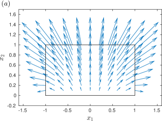
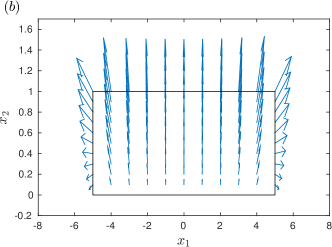
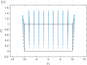
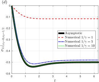
Figure 5: Panels (a)-(c) show numerical solutions for the deformation field $(u_{1},u_{2})$ to the macroscale equations (58)-(75) for different values of $1/\gamma=1,5,10$ respectively. Convergence to a one-dimensional deformation is clearly observed as $\gamma\rightarrow 0^{+}$. Panel (d) shows a comparison between $\sigma_{11}|_{x_{1}=0,x_{2}=1/2}(t)$ from the numerical simulations and the asymptotic analysis, i.e. (91).

4 The microscale problem

We now revisit the microscale problem, rescaling the governing equations about a generic individual electrode particle at $(x_{1},x_{2})=(x_{1,m},x_{2,n})$ somewhere in the bulk of the electrode by writing

(92) $$x_{2}-x_{2,n}=\lambda X_{2},\qquad x_{1}-x_{1,m}=\lambda X_{1},\qquad u_{1}=v_{1,m,n}+\lambda U_{1},\qquad u_{2}=v_{2,m,n}+\lambda U_{2}.$$

We aim to solve (34)-(54) for the microscale variables $X_{i}$, $U_{i}$ on a single periodic unit cell $-1/2<X_{1}<1/2$, $-1/2<X_{2}<1/2$. Boundary conditions on the microscale cell problem need to be chosen in order that the micro-solution is compatible with the one-dimensional solution to the macroscale problem (87). Since there is no macroscopic shear, we require $\sigma_{12}=0$ on $X_{1}=\pm 1/2$ and $X_{2}=\pm 1/2$. In addition, since there are no lateral macroscopic displacements, we require $U_{1}=0$ on $X_{2}=\pm 1/2$. On the other hand, averaging the 22 component of the microscopic strain over the unit cell, which yields the net relative displacement of the horizontal boundaries of the cell, should be also equal to the macroscopic strain, so that

$$\int_{-1/2}^{1/2}\frac{\partial U_{2}}{\partial X_{2}}\,dX_{2}=U_{2}\big{|}_{X_{2}=1/2}-U_{2}\big{|}_{X_{2}=-1/2}=\epsilon^{\mathrm{eff}}_{22}=\frac{\partial u_{2}^{\mathrm{eff}}}{\partial x_{2}}=2\ell(t).$$

Since we have not derived the effective coefficients of the macroscale problem, and therefore cannot accurately determine the macroscale strain $\epsilon^{\mathrm{eff}}_{22}$, we do not impose $\ell(t)$ directly but calculate it self-consistently using the condition that there is no normal macroscale stress in the vertical direction ($\sigma_{22}^{\mathrm{eff}}=0$), which implies

(93) $$\int_{-1/2}^{1/2}\sigma_{22}\,\mathrm{d}X_{1}=0\quad\mbox{ on }\quad X_{2}=\pm 1/2.$$

Finally we have the swelling condition that $U_{i}=X_{i}g(t)$ on the particle $\Gamma_{5}^{m,n}$.

The microscale problem we have derived is symmetric in both $X_{1}$ and $X_{2}$, so that we may solve it more efficiently by considering the quarter-cell domain, depicted in Figure 6, with boundary segments

(94) $$\Gamma_{1}^{\mathrm{mic}}=\{X_{1},X_{2}\,|\,r_{0}<X_{1}<1/2,X_{2}=0\},\qquad\Gamma_{2}^{\mathrm{mic}}=\{X_{1},X_{2}\,|\,X_{1}=1/2,0<X_{2}<1/2\},$$

(95) $$\Gamma_{3}^{\mathrm{mic}}=\{X_{1},X_{2}\,|\,0<X_{1}<1/2,X_{2}=1/2\},\quad\Gamma_{4}^{\mathrm{mic}}=\{X_{1},X_{2}\,|\,X_{1}=0,r_{0}<X_{2}<1/2\},$$

(96) $$\Gamma_{5}^{\mathrm{mic}}=\{X_{1},X_{2}\,|\,X_{1}>0,X_{2}>0,X_{1}^{2}+X_{2}^{2}=r_{0}^{2}\}.$$

Figure 6: Schematic of the geometry of the microscale problem.

The boundary and symmetry conditions are then

$$\mbox{on}\,\,\Gamma_{1}^{\mathrm{mic}}:$$

(97) $$U_{2}=0$$

(98) $$\sigma_{12}=0,$$

$$\mbox{on}\,\,\Gamma_{2}^{\mathrm{mic}}:$$

(99) $$U_{1}=0$$

(100) $$\sigma_{12}=0,$$

$$\mbox{on}\,\,\Gamma_{3}^{\mathrm{mic}}:$$

(101) $$U_{2}=\ell(t)$$

(102) $$\sigma_{12}=0,$$

$$\mbox{on}\,\,\Gamma_{4}^{\mathrm{mic}}:$$

(103) $$U_{1}=0$$

(104) $$\sigma_{12}=0,$$

$$\mbox{on}\,\,\Gamma_{5}^{\mathrm{mic}}:$$

(105) $$U_{1}=X_{1}g(t)$$

(106) $$U_{2}=X_{2}g(t),$$

where $\ell(t)$ is determined by the requirement that

(107) $$\int_{\Gamma_{3}^{\mathrm{mic}}}\sigma_{22}\,\mathrm{d}X_{1}=0.$$

Finally, we note that the condition (54) is automatically satisfied due to symmetry and also that there is no net torque on the particle, so that our earlier decision not to allow for rotations is justified.

Owing to the geometry, solution of the microscale problem must be obtained using numerical techniques. We employ the finite element method, and implement this approach using the open source software FreeFEM++ [28]. The problem has two non-standard features, namely: (I) the constitutive equations involve time derivatives of the stress- and strain-fields, and; (II) the problem is subject to an integral constraint, namely (107). The first of these difficulties is tackled by discretizing the governing equations in time using an explicit approximation; this leads to an elliptic boundary-value problem for the state variables at each time step that are of similar form to those for an elastic medium — information from the previous time step is retained in the form of source terms. The second difficulty is circumvented by embedding a code that solves the problem for a specified value of $\ell(t)$ (a tractable problem) within a root-finding loop that determines the value of $\ell(t)$ at the new time step that leads to a stress field satisfying (107). Since the variation of the average normal load on the top surface is a linear function of $\ell(t)$, only two ‘test’ problems need to be solved per time step in order to find the value of $\ell(t)$ satisfying (107). We now detail the method of numerical solution to this microscale problem.

4.1 Numerical approach

Before implementation in FreeFem++, the system of equations must be written in a suitable variational form. Given the non-standard nature of our problem, we briefly outline the procedure for deriving this variational formulation. First, we take the partial derivative of the force balance equation (34) with respect to time and then eliminate $\sigma_{ij}$ in favor of $\epsilon_{ij}$, $E$ and $S$ using equations (37)-(41). On doing so, and denoting a partial derivative in time with a dot, we arrive at

(108) $$\begin{split}\frac{\partial}{\partial x_{j}}\left(G_{2}G_{\tau}\dot{\epsilon}_{ij}+\epsilon_{ij}\right.\qquad\qquad\qquad\qquad\qquad\qquad\qquad\qquad\qquad\qquad\qquad\qquad\\ \left.+\delta_{ij}\left[(K_{2}K_{\tau}-G_{2}G_{\tau})\dot{E}-K_{2}K_{\tau}\dot{\beta}_{\mathrm{abs}}+(K_{1}-1)E-K_{1}\beta_{\mathrm{abs}}\right]\right)=0.\end{split}$$

This equation is then discretized explicitly in time using a forward Euler approximation, multiplied by a test function $v_{i}\in C^{\infty}_{0}(\Omega)$ and integrated by parts (in the usual way) to obtain the variational form

$$\int_{\Gamma}a_{1}\epsilon_{ij}(u^{(n+1)})v_{j}n_{i}+a_{2}\epsilon_{ij}(u^{(n)})v_{j}n_{i}+a_{3}E(u^{(n+1)})v_{i}n_{i}+a_{4}E(u^{(n)})v_{i}n_{i}\,dS$$

(109) $$-\int_{\Omega}a_{1}\epsilon_{ij}(u^{(n+1)})\epsilon_{ij}(v)+a_{2}\epsilon_{ij}(u^{(n)})\epsilon_{ij}(v)+2a_{3}E(u^{(n+1)})E(v)$$

$$+2a_{4}E(u^{(n)})E(v)-G_{\tau}\frac{\partial S^{(n)}}{\partial x_{i}}v_{i}\,d\Omega.$$

Here the superscripts denote the respective time levels, $\Delta t$ is the (small) time step and the coefficients ($a_{1}$ to $a_{4}$) are defined by the relations

(110) $$a_{1}=G_{2}G_{\tau},$$

(111) $$a_{2}=\Delta t-G_{2}G_{\tau},$$

(112) $$a_{3}=K_{2}K_{\tau}-G_{2}G_{\tau},$$

(113) $$a_{4}=\Delta t(K_{1}-1)-(K_{2}K_{\tau}-G_{2}G_{\tau}).$$

On using the boundary conditions (97)-(106) to simplify the boundary term, equation (109) can be viewed as a problem for the displacement (and in turn the strain) field for a given value of the volumetric stress at the previous time step $S^{(n)}$. An equation for the evolution of $S^{(n)}$ is obtained by discretizing (41) in time (again using the forward Euler method) to give

(114) $$\begin{split}S^{(n+1)}=\left(1-\frac{\Delta t}{K_{\tau}}\right)S^{(n)}+K_{2}E^{(n+1)}\qquad\qquad\qquad\qquad\qquad\qquad\qquad\qquad\\ +\left(\frac{K_{1}\Delta t}{K_{\tau}}-K_{2}\right)E^{(n)}-K_{2}\beta_{\mathrm{abs}}^{(n+1)}+\left(K_{2}-\frac{K_{1}\Delta t}{K_{\tau}}\right)\beta_{\mathrm{abs}}^{(n)}.\end{split}$$

A code that evolves (109) and (114) may then be implemented in FreeFem++ — a pseudo-code is included in algorithm 1.

  $t=0$

  $n=0$

  Define the initial conditions: $u_{i}^{(0)}=\epsilon_{ij}^{(0)}=E^{(0)}=S^{(0)}=L^{(0)}=0$

  repeat

     Advance time: $t=t+\Delta t$

     Define the first ‘test’ value of $\ell^{(n+1)}$: $\ell_{1}^{\prime}=\ell^{(n)}-0.1$

     Define the second ‘test’ value of $\ell^{(n+1)}$: $\ell_{2}^{\prime}=\ell^{(n)}+0.1$

     Solve (109) with $\ell^{(n+1)}=\ell_{1}^{\prime}$

     Evaluate the average normal load on $\Gamma_{\mathrm{mic}}^{3}$ for the first ‘test’ value: $F_{1}=\int_{\Gamma_{3}^{\mathrm{mic}}}\sigma^{(n+1)}_{yy}dS$

     Solve (109) with $\ell^{(k+1)}=\ell_{2}^{\prime}$

     Evaluate the average normal load on $\Gamma_{\mathrm{mic}}^{3}$ for the second ‘test’ value: $F_{2}=\int_{\Gamma_{3}^{\mathrm{mic}}}\sigma^{(n+1)}_{yy}dS$

     Compute the value of $\ell^{(n+1)}$ corresponding to zero load on $\Gamma_{\mathrm{mic}}^{3}$: $\ell^{(n+1)}=\ell_{2}^{\prime}-F_{2}((\ell_{2}^{\prime}-\ell_{1}^{\prime})/(F_{2}-F_{1}))$

     Solve (109) for $u_{i}^{(n+1)}$, $\epsilon_{ij}^{(n+1)}$ and $E^{(n+1)}$ using $\ell^{(n+1)}$

     Compute $S^{(n+1)}$ using (114)

     Advance the index: $n=n+1$

  until $t>T_{end}$

Algorithm 1 The pseudo-code for the evolution on the microscopic scale.

All the usual diagnostic checks were carried out to ensure that the method was performing as expected. In order to ensure errors were acceptably small, the number of elements (and the size of the time step) were increased (decreased) until no appreciable changes were observed in the solutions. Typically, we found that using $P2$ elements, meshing the domain with approximately $100\times 100$ elements, and taking the time step $\Delta t=10^{-3}$ gave solutions which were converged to 4 significant digits of accuracy.

4.2 Deformation driven by electrolyte absorption

In this section we consider forcing deformation in the microscale problem by allowing the polymer binder to absorb electrolyte, i.e. via the function $\beta_{\mathrm{abs}}$ in (41) — the volumetric change of the electrode particle is taken to be zero. In line with the estimates given in §2.5 we take

(115) $$\beta_{\mathrm{abs}}=\frac{1}{2}\tanh(t),\qquad g(t)=0\qquad r_{0}=\frac{1}{2},\qquad G_{\tau}=0.02,$$

(116) $$G_{2}=3,\qquad K_{\tau}=0.02,\qquad K_{1}=1,\qquad K_{2}=3,$$

so that the absorption of the electrolyte causes the volume of the polymer (corresponding to zero stress) to increase by 50% for large time.

The stress fields generated at the end of the simulation are shown in Figure 7, the deformation field at the end of the simulation (at $t=T_{end}=10$) is shown in Figure 8 whilst the evolution of both $\ell(t)$ and the normal stresses at the points $P_{1}$ and $P_{2}$ (as defined in Figure 6) are shown in Figure 9. We see that after swelling, the normal stress at the top (and bottom) of the electrode particle is tensile whereas at the right-hand (and left-hand) side it is compressive. This indicates that deformations induced by electrolyte absorption are likely to cause preferential delamination of the polymer binder from the top (and bottom) of the particle surfaces. This result can be understood intuitively by considering a growing solid medium confined within two rigid vertical walls. If the material were to expand without constraint it would dilate uniformly, however because it is confined in the horizontal direction, it has no choice but decrease its internal stresses by flowing/deforming predominantly in the vertical direction — see panel (a) of Figure 8. If this material were also to contain a circular rigid inclusion (e.g. an electrode particle), then the description above is still appropriate and the growing material would therefore try to pull away from the circular inclusion at its top and bottom surface as it flows/deforms.

In Figure 9 we see that for the parameter choices given in (115)-(116) the increase in stress at the point P1 (and decrease at point P2) is monotonic in time and saturates to a constant. The constant to which these quantities tend is controlled by: (i) the long time behavior of the growth function $\beta_{\mathrm{abs}}(t)$, and; (ii) the long term moduli of the polymer, $K_{1}$ — corresponding to $G_{1}^{*}$ and $K_{1}^{*}$ in dimensional quantities. If one were designing a binder specifically to minimize the amount of damage caused by polymer swelling one could therefore try to minimize the degree of absorption and/or the long term moduli.

In addition to the results shown in Figures 7, 8 and 9, other simulations with different material constants were also carried out. It is possible to qualitatively change the monotonic behavior seen in Figure 9 if the time scales for absorption and viscoelastic relaxation become comparable, i.e. if $G_{\tau}$ or $K_{\tau}=O(1)$. In such regimes, transient behaviour may occur with the magnitude of the normal stresses at the point $P_{1}$ and $P_{2}$ increasing to large values before relaxing back down to those predicted by their long term moduli. In the context of mitigating mechanical damage this is an undesirable situation. Thus, one further practical recommendation is to ensure that the viscoelastic relaxation timescales remain much shorter than those for electrolyte absorption thereby taking advantage of the tendency of viscoelastic materials to flow in order to minimize their internal stresses. As far as the authors are aware, most polymers used for binder do take a long time to absorb electrolyte (at least several hours) and therefore it seems unlikely that this viscoelastic relaxation would ever be observed in practice.

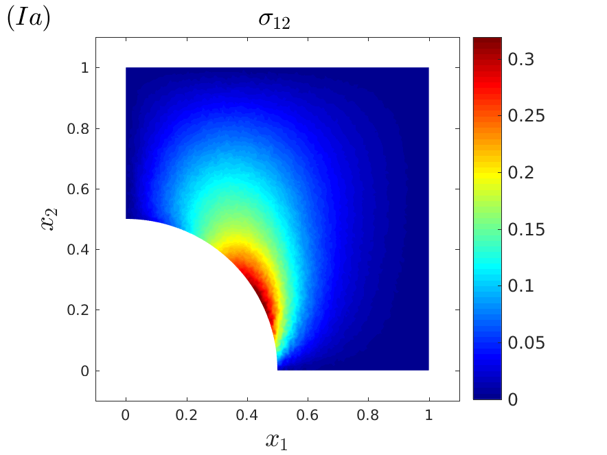
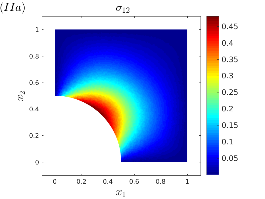
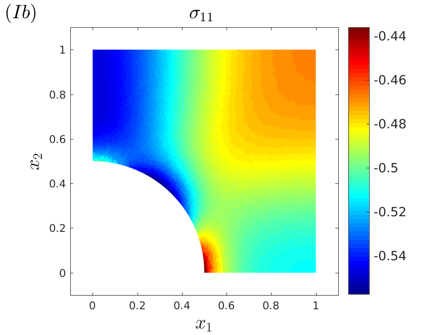
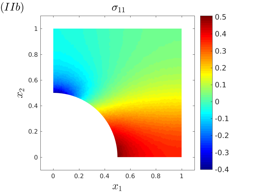
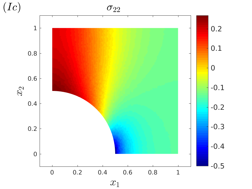
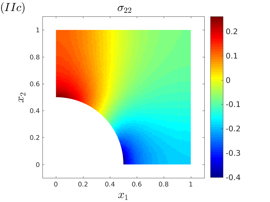
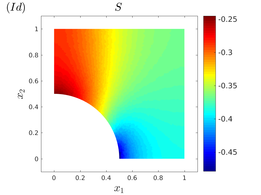
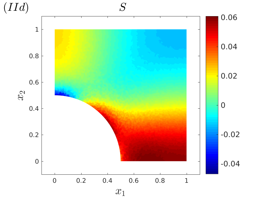
Figure 7: Column (I) shows the different components of the stress field at the end of the simulation defined by (115)-(116), i.e. after the binder has absorbed electrolyte and swelled. Here, we see that $\sigma_{22}|_{P_{1}}>0$ (binder in tension) whereas $\sigma_{11}|_{P_{2}}<0$ (binder in compression). Column (II) shows analogous plots at $t=\pi$ for the simulation defined by (117)-(118), i.e. for deformations driven by cycling in a cathode at the peak of discharge. Here, we see that both $\sigma_{22}|_{P_{1}},\sigma_{11}|_{P_{2}}>0$ (binder in tension).

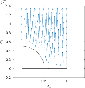
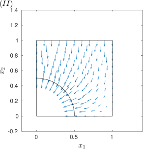
Figure 8: Panel (I) shows the deformation field at the end of the simulation defined by (115)-(116), i.e. after the binder has absorbed electrolyte and swelled. Panel (II) shows the deformation field at $t=\pi$ for the simulation defined by (117)-(118), i.e. for deformations driven by cycling in a cathode at the peak of discharge. Arrow lengths have been normalized in each plot individually.

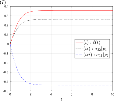
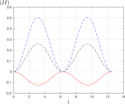
Figure 9: The evolution of: (i) $\ell(t)$, the vertical displacement on the top of the unit cell $\Gamma_{3}^{\mathrm{mic}}$; (ii) $\sigma_{22}|_{P_{1}}$, the normal stress at the point $P_{1}$, and; (iii) $\sigma_{11}|_{P_{2}}$, the normal stress at the point $P_{2}$. Panel (I) shows the results for the simulation defined by (115)-(116), i.e. for deformations driven by electrolyte absorption, whereas panel (II) shows the results for the simulation defined by (117)-(118), i.e. for deformations driven by cycling.

4.3 Deformation driven by electrode particle swelling

Here, we investigate the evolution as the electrode particle changes its volume. We study a situation analogous to the images shown in Figure 2, i.e. a cathode in which the particles are at their largest at the time of manufacture; as the device is discharged the cathode particles shrink and then at some later time, as the device is re-charged, the cathodic active material grows. We base our initial simulation on electrode particles composed of NMC and, in line with the discussion in §2.5, we take

(117) $$\beta_{\mathrm{abs}}=0,\qquad g(t)=\frac{\cos(t)-1}{10},\qquad r_{0}=\frac{1}{2},\qquad G_{\tau}=0.02,$$

(118) $$G_{2}=3,\qquad K_{\tau}=0.02,\qquad K_{1}=1,\qquad K_{2}=3.$$

The components of the stress field at the end of the simulation (at $t=T_{end}=4\pi$), i.e. after two complete cycles, are shown in the right column of Figure 7, the corresponding deformation field is shown in Figure 8 whilst the evolution of the normal stress at the points $P_{1}$ and $P_{2}$ on the surface of the electrode particle is shown in Figure 9. In contrast to the deformations driven by electrolyte absorption, these electrode particle-induced deformations cause tension in the binder at all positions on the particle surface. Further, the normal stress (directed outward) at the right-hand (and left-hand) sides of the electrode particle are larger than those at the top (and bottom), indicating that volumetric changes in the electrode particles are likely to drive delamination of the binder at the left and right edges of the electrode particle more strongly. The reasons for this are straightforward to understand: throughout the cycle the particles are smaller than their original size and therefore the surrounding polymer material is in tension. The size of this tension is larger at the left- and right-hand sides, because the adjacent sides of the unit cell are fixed, whereas the top (and bottom) of the unit cell can deform thereby reducing the tension.

Since these simulation were based on electrochemical cycling taking place on the scale of tens of hours (comparable to the timescale for electrolyte absorption), the viscoelastic relaxation is not clearly observed. The size of the stresses are therefore primarily controlled by the material parameter $K_{1}$ — or $K_{1}^{*}$ and $G_{1}^{*}$ in dimensional form — and the size of the volumetric changes of the particle $g(t)$.

It is relevant to also consider the evolution when the cathode is cycled more aggressively. To do so we keep all parameters identical to those shown in (117)-(118), but time is rescaled so that the relaxation timescales $G_{\tau}=K_{\tau}=1$. Thus, the cycling rate has been increased by a factor of 50 so that a cycle now takes only several minutes (rather than hours). The evolution of the normal stresses at $P_{1}$ and $P_{2}$ as well as $\ell(t)$ are shown in Figure 10. The viscoelastic relaxation is now apparent — the stresses are no longer close to zero at the end of each cycle. When the particle has returned to its original size, the normal stresses have become negative so that the surrounding binder is under compression; a beneficial configuration in the context of mitigating delamination. This is observed because the binder is in tension mid-cycle (the particle is smaller than originally). Thus, when the particle returns to its original size, the binder has undergone creep so that its zero stress state corresponds to a configuration with a smaller embedded electrode particle. This creeping effect is stronger at $P_{2}$ than at $P_{1}$, because the vertical edges of the unit cell are fixed whereas the top (and bottom) can move thereby causing the binder at the top (and bottom) to be under a decreased load leading to reduced creep.

A similar pair of simulations (one slow cycling and one fast cycling) were also carried out for an anode. The difference between the anode and cathode is that, for an anode, the electrode particles are initially delithiated (at their smallest) and their volume then increases as the cell is discharged. Simulations for the anode were carried out with $g(t)=(1-\cos(t))/10$. The evolution of the stresses at $P_{1}$ and $P_{2}$ as well as $\ell(t)$ are shown in panels (a) (for slow cycling with $K_{\tau}=G_{\tau}=0.02$) and (b) (for fast cycling with $K_{\tau}=G_{\tau}=1$) of Figure 11. For the anode we find that the slow cycling protocol is unlikely to drive any delamination at all — mid-cycle the electrode particle is larger than is was originally and therefore the surrounding binder is in compression. Since the cycling timescale is much slower than the relaxation timescale, very little creep occurs and so when the particle returns to its original position the stresses on the surface are negligibly small. Interestingly, and in contrast to the cathode, the creep that is observed for the more aggressive C-rate (see panel (b) of Figure 11) is likely to cause delamination rather than prevent it. Here, when the particle returns to its smallest (original) size the binder has crept such that it is now under tension. Thus, fast cycling rates are likely to increase the delamination damage in the anode. For similar reasons to those discussed above, this creep has a greater effect on the right- and left-hand sides than on the top and bottom of the particle surfaces.

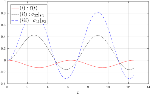
Figure 10: The evolution of: (i) $\ell(t)$, the vertical displacement of the top of the unit cell $\Gamma_{3}^{\mathrm{mic}}$; (ii) $\sigma_{22}|_{P_{1}}$, the normal stress at the point $P_{1}$, and; (iii) $\sigma_{11}|_{P_{2}}$, the normal stress at the point $P_{2}$. The result shown is for a cathode under aggressive cycling conditions as discussed in the penultimate paragraph of §4.3.

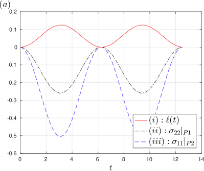
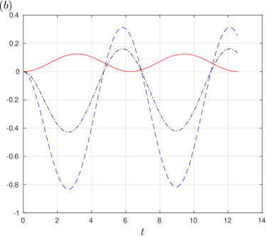
Figure 11: The evolution of: (i) $\ell(t)$, the vertical displacement of the top of the unit cell $\Gamma_{3}^{\mathrm{mic}}$; (ii) $\sigma_{22}|_{P_{1}}$, the normal stress at the point $P_{1}$, and; (iii) $\sigma_{11}|_{P_{2}}$, the normal stress at the point $P_{2}$. The results shown are for anodes under slow (panel (a)) and fast (panel (b)) electrochemical cycling as discussed in the final paragraph of §4.3.

5 Discussion and conclusions

We have developed a continuum mechanics model capable of predicting the mechanical response of porous lithium-ion battery electrodes to both (i) the swelling of the polymer binder on absorption of electrolyte and; (ii) cyclic swelling/contraction of the electrode particles as the battery is charged and discharged. The main goal of this work has been to understand the causes of delamination of the binder from the electrode particle surfaces as these devices are assembled and used. We have shown that for typical electrodes, the permeability is large enough that, on the time- and length-scales of interest, pressure gradients within the electrolyte equilibrate almost instantaneously, and do so without inducing any significant stress within the surrounding porous skeleton. Crucially, this decouples the fluid and solid components of the model, and reduces the problem to one of predicting the mechanical state of the polymer binder from a system of viscoelastic equations only. In order to account for the complex geometry of a realistic electrode we employed a multiscale approach to solving the decoupled model. First, the governing equations were upscaled, in an ad-hoc manner, to give an approximate homogeneous problem applicable on the electrode lengthscale. The solution of the resulting macroscopic problem was found to be almost entirely one-dimensional throughout the bulk of the electrode — a consequence of its slender geometry and its bonding to a rigid current collector. This simple solution on the electrode lengthscale was used to infer boundary conditions for the microscale problem about an individual electrode particle. The solution of this microscale problem was determined numerically using finite elements techniques on a representative ‘unit cell’.

We demonstrated that the two different driving mechanisms, polymer swelling and electrode particle volume changes, cause distinct modes of deformation. Swelling of the polymer, caused by absorption of the electrolyte, leads to large tensile stresses on the top and bottom surfaces of the electrode particles which are likely to lead to delamination from these surfaces. Cycling of the cathode, which is constructed from electrode particles in their fully-lithiated (largest) state, leads to tensile stresses along the surface of the particle, but most strongly on its sides. This is expected to lead to delamination occurring predominantly on the particle sides which contrasts with the expected mode of delamination due to binder swelling (along the top and bottom particle surfaces). In anodes, on the other hand, in which the particles are initially delithiated (smallest), cycling at slow rates, where the timescale for (dis-)charge are very much longer than the viscoelastic relaxation, is likely to cause little or no delamination. In high current applications, however, it is possible to reach regimes where the creep of the polymer becomes important and delamination can be induced in the anode microstructure. These insights, combined with suitable microscopy techniques, allow educated postmortems of real devices to be carried out. If delamination is seen mainly at the upper and lower surfaces of the electrode particles, then binder swelling is likely the primary cause whereas if delamination has occurred at the lateral edges it is more likely a result of cell cycling.

In cathodes delamination caused by binder swelling and cell cycling in low current applications (where time scales for cycling are much longer than those for viscoelastic relaxation) can be mitigated by: (i) decreasing the volumetric changes associated with binder swelling and electrode particle swelling/contraction and (ii) by decreasing the long-term moduli of the polymer — the other material properties of the binder have little or not effect. For high current applications, the delamination induced in the anode can also be mitigated by using the tactics discussed above, or by decreasing either the short-term moduli or further decreasing the characteristic relaxation time of the polymer.

Returning for a moment to the images shown at the start of this study — see Figure 2 — we can now rationalize the different stages of morphological deterioration. In panel (a), prior to soaking in electrolyte, we see that the binder is well attached to the electrode particle surfaces. In panel (b), after electrolyte immersion but before cycling, we see significant delamination from the upper and lower parts of the electrode particle surfaces only. A simple visual inspection of panel (c) also reveals large regions of delamination running left to right. However, a more detailed analysis of these same images was carried out in [19], and there it was found that a measurable increase in the amount of delamination (around 5% in terms of electrode particle surface area) had occurred as a direct result of the electrochemical cycling stages. All three of these observations are consistent with the results of our model. The cycling stages caused significantly less damage than the swelling of the polymer for the electrodes shown in Figure 2. This is likely due to the NMC active material which only changes its volume a small amount ($\sim$2-4%) on (de-)lithiation. However, we do emphasize that for other chemistries, particularly newer silicon-based materials, which can exhibit extremely large volumetric expansions, the mechanical damage caused by active material swelling could be far more significant.

In [20] the framework developed here has already been used to explore the effects of alterations in particle shape and differing polymer rheology. Perhaps the most significant result in [20] was the demonstration that the size of the deterimental tensile normal stresses on the top and bottom surfaces of the particles caused by binder swelling can be reduced by using non-circular particles, e.g. ellipses, and aligning the longer edges of the particles in planes parallel with the CC. On the one hand this distributes the damaging tensile stress over a larger area, thereby reducing its size, but a larger area is then exposed to this relatively smaller stress. Before comments can be made on optimal particle shape, it is therefore crucial to understand the size of the threshold stress required to cause delamination. Other interesting open questions that remain to be addressed include: (i) formalizing the upscaling arguments used in §3; (ii) using the model and methods developed here to discern the effects of altering the packing of the electrode particles. Results on both these fronts will be reported in the near future.

References

- [1] Y. Abousleiman, A. H. D. Cheng, C. Jiang & J. C. Roegiers. Poroviscoelastic analysis of borehole and cylinder problems. Acta Mechanica, 119:199–219 (1996).
- [2] N. Balke, S. Jesse, A. N. Morozovska, E. Eliseev, D. W. Chung, Y. Kim, L. Adamczyk, R. E. Garcia & S. V. Kalinin. Nanoscale mapping of ion diffusion in a lithium-ion battery cathode. Nature Nanotechnology, 5:749. (2010).
- [3] A. J. Bard & L. R. Faulkner. Electrochemical methods: fundamentals and applications, 2nd edition.
- [4] M. A. Biot. Theory of deformation of a porous viscoelastic anisotropic solid. J. Appl. Phys., 27:459 (1956).
- [5] H. Buqa, D. Goers, M. Holzapfel, M.E. Spahr & P. Novak High rate capability of graphite negative electrodes for lithium-ion batteries J. electrochem. Soc., 152: A474-A481 (2005).
- [6] J. Cannarella & C. B. Arnold. State of health and charge measurements in lithium-ion batteries using mechanical stress. J. Power Sources, 269:7–14. (2014).
- [7] J. Cannarella & C. B. Arnold. Stress evolution and capacity fade in constrained lithium-ion puch cells. J. Power Sources, 245:745–751. (2014).
- [8] P. C. Carman. Fluid flow through granular beds. Transactions, Institution of Chemical Engineers, London, 15:150–166. (1937).
- [9] J. Chakraborty, C. P. Please, A. Goriely & S. J. Chapman. Combining mechanical and chemical effects in the deformation and failure of a cylindrical electrode particle in a Li-ion battery. Int. J. Solids and Struc., 54:66–81. (2015).
- [10] J. Chakraborty, C. P. Please, A. Goriely & S. J. Chapman. Influence of constraints on axial growth reduction of cylindrical Li-ion battery electrode particles. J. Power Sources., 279:746–758 (2015).
- [11] L. Chen, X. Xie, J. Xie, K. Wang & J. Yang. Binder effect on cycling performance of silicon/carbon composite anodes for lithium ion batteries. J. Appl. Electrochem., 36(10):1099–1104 (2006).
- [12] F. Ciucci & W. Lai. Derivation of Micro/Macro Lithium Battery Models from Homogenization. Transp. Porous Med., 88, 249–270 (2011).
- [13] D. A. Cogswell & M. Z. Bazant. Coherency strain and the kinetics of phase separation in LiFePO4 nanoparticles. ACS Nano, 6(3):2215–2225. (2012).
- [14] J. R. Dahn. Phase diagram of LixC6. Phys. Rev. B, 44:9170. (1991).
- [15] C. V. Di Leo, E. Rejovitzky & L. Anand. A Cahn-Hilliard-type phase-fluid theory for species diffusion coupled with large elastic deformations: application to phase-separating Li-ion electrode materials. J. Mech. Phys. Solids, 70:1–29. (2014).
- [16] M. Doyle and J. Newman. Analysis of capacity-rate for lithium batteries using simplified models of the discharge process. J. Appl. Electrochem., 27:846–856, 1996.
- [17] M. Doyle & J. Newman. Comparison of modeling predictions with experimental data from plastic lithium ion cells. J. Electrochem. Soc., 143:1890–1903, 1996.
- [18] W Flügge. “Viscoelasticity”, Springer-Verlag, Heidelberg, Berlin (1975).
- [19] J. M. Foster, A. Gully, H. Liu, S. Krachkovskiy, Y. Wu, S. Schougaard, M. Jiang, G. Goward, G. A. Botton & B. Protas. A homogenization study of the effects of cycling on the electronic conductivity of commercial lithium-ion battery cathodes. J. Phys. Chem., 119(22):12199–12208, 2015.
- [20] J. M. Foster, X. Huang, M. Jiang, S. J. Chapman, B. Protas & G. Richardson. Causes of binder damage in porous battery electrodes and strategies to prevent it. J. Power Sources, 350:140–151. (2017).
- [21] A. Fowler. “Mathematical models in the applied sciences”, Cambridge University Press, Cambridge (1997).
- [22] T. F. Fuller, M. Doyle, J. Newman. Relaxation phenomena in lithium-ion insertion cells. J. Electrochem. Soc. 143:982–990, 1994.
- [23] T. F. Fuller, M. Doyle and J. Newman. Simulation and optimisation of the dual lithium insertion cell. J. Electrochem. Soc., 141:1–10, 1994.
- [24] G. Y. Gor, J. Cannarella, J. H. Prevost & C. B. Arnold. A model for the behaviour of battery separators in compression at different strain/charge rates. J. Electrochem. Soc., 161(11):F3065–F3071. (2014).
- [25] G. Y. Gor, J. Cannarella, C. Z. Leng, A. Vishnyakov & C. B. Arnold. Swelling and softening of lithium-ion battery separators in electrolyte solvents. J. Power Sources, 294:167–172. (2015).
- [26] A. M. Grillet, T. Humplik, E. K. Stirrup, S. A. Roberts, D. A. Barringer, C. M. Snyder, M. R. Janvrin & C. A. Apblett. Conductivity degradation of polyvinylidene fluoride composite binder during cycling: measurements and simulations or lithium-ion batteries. J. Electrochem. Soc. 163(9):A1859–A1871 (2016).
- [27] A. Gully, H. Liu, S. Srinivasan, A. K. Sethurajan, S. Schougaard & B. Protas. Effective transport properties of porous electrochemical materials – a homogenization approach. J. Electrochem. Soc., 161(8):E3066–E3077. (2014).
- [28] F. Hecht. New development in FreeFem++. J. Num. Math., 20(3-4):251–265 (2012).
- [29] J. Heelan, E. Gratz, Z. Zheng, Q. Wang, M. Chen, D. Apelian & Y. Wang. Current and prospective Li-ion bttery recycling and recovery processes. J. Min. Met. Mat. S., 68(10):2632–2638. (2016).
- [30] M. Kerlau, M. Marcinek, V. Srinivasan & R. M. Kostecki. Studies of local degradtion phenomena in composite cathodes for lithium-ion batteries. Electrochimica Acta, 52:5422–5439. (2007).
- [31] J. Kozeny. Ueber kapillare Leitung des Wassers im Boden. Sitzungsber Akad. Wiss., 136(2a):271–306. (1927).
- [32] J. Li, C. Daniel & D.Wood. Materials processing for lithium-ion batteries J. Power Sources, 196: 2452–2460 (2011).
- [33] H. Liu, J. M. Foster, A. Gully, S. Krachkovskiy, M. Jiang, Y. Wu, X. Yang, B. Protas, G. Goward & G. A. Botton. Three-dimensional investigation of cycling-induced microstructural changes in lithium-ion battery cathodes using focused ion beam/scanning electron microscopy. J. Pow. Sou., 306:300–308 (2016).
- [34] G. Liu, H. Zheng, X. Song & V.S. Battaglia. Particles and polymer binder interaction: a controlling factor in lithium-ion electrode performance. J. Electrochem. Soc., 159:A214–A221 (2012).
- [35] X. M. Liu & C. B. Arnold. Effects of cycling ranges on stress and capacity fade in lithium-ion puch cells. J. Electrochem. Soc., 163(13):A2501–A2507. (2016).
- [36] A. Magasinski, B. Zdyrko, I. Kovalenko, B. Hertzberg, R. Burtovvy, C. F. Huebner, T. F. Fuller, I. Luzinov & G. Yushin. Toward efficient binders for Li-ion battery Si-anodes: polyacrylic acid. Applied Materials and Interfaces, 2(11):3004–3010 (2010).
- [37] T. Maxisch & G. Ceder. Elastic properties of olivine LiFePO4 from first principles. Phys. Rev. B, 73:174112-1–174112-4. (2006).
- [38] J. S. Newman. Electrochemical systems, 3rd edn. Prentice Hall, New Jersey, 2004.
- [39] T. Ohzuku & A. Ueda. Solid-state redox reactions of LiCoO2 (Rm) for 4 volt secondary lithium cells. J. Electrochem. Soc., 141(11):2972–2977. (1994).
- [40] J. Ott, B. Volker, Y. Gan, R. M. McMeeking & M. Kamlah. A micromechanical model for effective conductivity in granular electrode structures. Acta Mechanica Sinica, 29(5):682–698 (2013).
- [41] H. Park, B. Kong & E. Oh. Effect of high adhesive polyvinyl alcohol binder on the anodes of lithium ion batteries. Electrochemistry Communications, 13(10):1051–1053 (2011).
- [42] C. Peabody & C. B. Arnold. The role of mechanically induced separator creep in lithium-ion battery capacity fade. J. Power Sources, 196:8147–8153. (2011).
- [43] M. B. Pinson & M. Z. Bazant. Theory of SEI formation in rechargable batteries: capacity fade, accelerated aging and lifetime prediction. J. Electrochem. Soc., 106(2):A243–A250. (2013).
- [44] Y. Qi & S. J. Harris. In situ observation of strains during lithiation of a graphite electrode. J. Electrochem. Soc., 157(6):A741–A747, 2010.
- [45] Y. Qi, H. Guo, L. G. Hector Jr. & A. Timmons. Threefold increase in the YOung’s modulus of graphite negative electrode during lithium intercalation. —em J. Electrochem. Soc., 157(5):A558–A566. (2010).
- [46] R. Reynier, R. Yazami & B. Fultz. XRD evidence of macroscopic composition inhomogenaities in the graphite-lithium electrode. J. Power Sources, 165:616. (2007).
- [47] G. Richardson & S. J. Chapman, Derivation of the bidomain equations for a beating heart with a general microstructure. SIAM J. Appl. Math. 71: 657-675 (2011).
- [48] G. Richardson, G. Denuault & C. P. Please, Multiscale modeling and analysis of lithium-ion battery charge and discharge. J. Eng. Math. 72, 41:1-772 (2012).
- [49] S. A. Roberts, H. Mendoza, V. E. Brunini, B. L. Trembacki, D. R. Noble & A. M. Grillet. Insights into lithium-ion battery degradation and safety mechanisms from mesoscale simulations using eperimentally reconstructed microstructures. J. Electrochem. Energy Conversion and Storage 13(3), 031005 (2016).
- [50] V. A. Sethuraman, N. Van Winkle, D. P. Abraham, A. F. Bower & P. R. Guduru. Real-time stress measurements in lithium-ion battery negative-electrodes. J. Power Sources, 206:334–342. (2012).
- [51] Sigma-Aldrich, Lithium hexafluorophosphate solution datasheet.
- [52] J. Vetter, P. Novak, M. R. Wagner, C. Veit, K. C. Moller, J. O. Besenhard, M. Winter, M. Wohlfahrt-Mehrens, C. Vogler & A Hammouche. Ageing mechanisms in lithium-ion batteries. Journal of Power Sources, 147:269–281. (2005).
- [53] A. Vinogradov & F. Holloway. Electro-mechanical properties of the piezoelectric polymer PVDF. Ferroelectrics, 226(1):169–181. (1999).
- [54] H. F. Wang. Theory of linear poroelasticity: with applications to geomechanics and hydrogeology. Princeton University Press.
- [55] Q. Wang, P. Ping, X. Zhao, G. Chu, J. Sun & C. Chen. Thermal runaway caused fire and explosion of lithium ion battery. Journal of Power Sources, 208:210–224. (2012).
- [56] M. S. Whittingham. Lithium batteries and cathode materials. Chem. Rev., 104:4271. (2004).
- [57] W. H. Woodford, Y. Chiang & W. C. Carter. “Electrochemical shock” of intercalation electrodes: a fracture mechanics analysis. J. Electrochem. Soc., 157(10):A1052–A1059. (2010).
- [58] W. Wu, X. Xiao, M. Wang & X. Huang. A microstructural resolved model for the stress analysis of lithium-ion batteries. J. Electrochem. Soc., 161(5):A803—A813 (2014).
- [59] N. Yabuuchi & T. Ohzuku. Novel lithium insertion material of LiCo1/3Ni1/3Mn1/3O2 for advanced lithium-ion batteries. J. Power Sources, 119-121:171–174. (2003).
- [60] M. Yoo, C.W. Frank, S. Mori & S. Yamaguchi. Effect of poly (ninylidene fluoride) binder crystallinity and graphite structure on the mechanical strength of the composiite anode in a lithium ion battery. Polymer, 44: 4197-4204 (2003).
- [61] M. Yoshio, R. J. Brodd & A Kozawa. Lithium-ion batteries: science and teachnologies (Springer).
- [62] C. Zener Elasticity and anelasticity of metals. University Chicago Press. (1948).
- [63] Y. Zeng & M. Z. Bazant. Phase separation dynamics in isotropic ion-intercalation particles. SIAM J. Appl. Math., 74(4):980–1004. (2014).
Acknowledgements
Thanks to S. Krachkovskiy and G. Goward for constructing and cycling the cells, and to H. Liu and G. Botton for providing the microscopy images used in this study. Thanks also to K. Harris, X. Huang, J. H. Kim, I. Halalay, C. P. Please and I. Danaila for stimulating discussions regarding this work. The electron microscopy data included in this paper was acquired at the Canadian Centre for Electron Microscopy, a national facility supported by the Natural Sciences and Engineering Research Council of Canada (NSERC) and McMaster University. Funding for this research was provided by Automotive Partnership Canada (APC) and General Motors of Canada.