Gravitational collapse of massless scalar field in $f(R)$ gravity

Abstract

We study the spherically symmetric gravitational collapse of massless scalar matter field in asymptotic flat spacetime in the Starobinsky $R^{2}$ gravity, one specific model in the $f(R)$ gravity. In the Einstein frame of $f(R)$ gravity, an additional scalar field arises due to the conformal transformation. We find that besides the usual competition between gravitational energy and kinetic energy in the process of gravitational collapse, the new scalar field brought by the conformal transformation adds one more competing force in the dynamical system. The dynamical competition can be controlled by tuning the amplitudes of the initial perturbations of the new scalar field and the matter field. To understand the physical reasons behind these phenomena, we analyze the gravitational potential behavior and calculate the Ricci scalar at center with the change of initial amplitudes of perturbations. We find rich physics on the formation of black holes through gravitational collapse in $f(R)$ gravity.

I Introduction

The dynamical evolution of an isolated system in general relativity is governed by the Einstein-matter equations and it can end up in qualitatively different stable end states, either with the formation of a single black hole in collapse or completely dispersion of the mass-energy to infinity. For a massless scalar field in spherical symmetry, these are the only possible end states. The fate of the evolution of an isolated system in general relativity is determined by the dynamical competition which can be controlled by tuning parameters in the initial conditions Christodoulou_87 ; Christodoulou_91 ; Christodoulou_94 ; Wald_97 . If the parameter $p$ is less than some critical value $p_{\star}$, the kinetic energy of the field will completely disperse the mass-energy of the system to infinity; while if $p>p_{\star}$, the gravitational potential dominates and a black hole forms. It is intriguing that the phenomenology of existing a threshold of black hole formation becomes apparent and universal in a large class of collapse models in general relativity. This phenomenology, which includes scaling, self-similarity and universality, is analogous to the critical behavior in statistical mechanics. Critical phenomena in gravitational collapse in Einstein gravity were first discovered by Choptuik in the model of a spherical symmetric, massless scalar field minimally coupled to general relativity Choptuik_92 ; Choptuik_93 ; Choptuik_94 . Important results of gravitational collapse in the best-studied models have been reviewed in spherical symmetry in asymptotically flat spacetimes Choptuik_98 ; WangAn_01 ; Gundlach_07 . The gravitational collapse in de Sitter Einstein gravity has also been investigated in Hod_97 ; Iwashita_05 ; Zhang_15 . It was found that the positive cosmological constant enhances the effect of dispersion and makes the black hole formation more difficult compared with the corresponding asymptotically flat spacetime. Recently with the growing interest in anti-de Sitter (AdS) spacetimes, a lot of works have been done on the gravitational collapse in AdS space Bizon_10 ; Garfinkle_11 ; Dias_11 ; Liebling_12 ; Wu_12 ; Maliborski_12 ; Buchel_12 ; Maliborski_13 ; Craps_14 ; Balasubramanian_14 ; Cai_15 ; Cai_16 ; Deppe_14 . The AdS spacetime is in stark contrast to asymptotically flat and de Sitter spacetimes because of the AdS boundary which needs to input suitable boundary conditions in order to make the evolution of the dynamical system well defined. It was claimed that in AdS space black hole can always be formed under arbitrarily small generic perturbations due to the interplay of local nonlinear dynamics and the non-local kinematic effect of the AdS reflecting boundary Bizon_10 . While in Einstein-Gauss-Bonnet AdS gravity, it was found that black holes will not form dynamically if the total mass/energy content of the spacetime is too small Deppe_14 . Further investigations of gravitational collapse in AdS spacetime are still being carried out.

Most phenomenologies of gravitational collapse were disclosed in Einstein gravity. It is of great interest to ask questions on how about the stability of the spacetime in modified gravity, whether black holes can be formed through gravitational collapse in modified gravity and whether there is a black hole threshold in the space of initial data in modified gravity. The attempts to study the collapse of a free scalar field in the Brans-Dicke model of gravity were carried out in Liebling_96 ; Chiba_96 . It was found that at the critical point of black hole formation, the model admits two distinctive solutions depending on the value of the coupling parameter between the Brans-Dicke field and matter, which admits one solution to be discretely self-similar and the other to exhibit continuous self-similarity. Recently the study of gravitational collapse has been extended to a more general gravity theory, the Horndeski theory Koutsoumbas_15 . However to avoid the complexity, the authors concentrated their attention on a homogeneous time-dependent scalar field coupling to curvature and Einstein tensor. In this paper, we are going to examine the gravitational collapse in a specific $f(R)$ gravity model, the Starobinsky $R^{2}$ gravity. The evidences of existing spherically symmetric black holes in $f(R)$ gravity were reported for example in Canate_15 . However the dynamical process of forming black holes in $f(R)$ gravity through gravitational collapse is not clear. In the cosmological context, the $f(R)$ gravity can accommodate the early Starobinsky_80 or late time Carroll_04 acceleration of the universe. This implies that $f(R)$ gravity can produce some kind of repulsive force similar to that of inflaton or dark energy in the Einstein gravity. Whether such kind of repulsive effect in $f(R)$ gravity can hinder the gravitational collapse and the formation of black holes is a question to be answered. Thus we have strong motivation to generalize the formalism of studying the gravitational collapse well established in general relativity to the $f(R)$ gravity to examine the dynamical competitions in the gravitational collapse, disclose the threshold of black hole formation and compare with corresponding properties in the Einstein gravity.

The studies on gravitational collapse in $f(R)$ gravity have been reported from some aspects. Fluid gravitational collapse in $f(R)$ gravity was examined in Sharif_10 ; Sharif_13 ; Sharif_14 ; Kausar_14 ; Chakrabarti_16 . The gravitational collapse of a charged black hole in $f(R)$ gravity was studied in Hwang_11 by using double-null formalism and the mass inflation of the Cauchy horizon was examined. In Cembranos_12 , the authors analyzed a general $f(R)$ model with uniformly collapsing cloud of self-gravitating dust particles. Dark matter halo formation was studied in Kopp_13 . Spherical scalar collapse in $f(R)$ gravity towards a black hole formation was simulated in Guo_13 . The gravitational collapse of massive stars in $f(R)$ gravity was analyzed in Goswami_14 . Furthermore employing the double-null formalism, spherical scalar collapse for the Starobinsky $R^{2}$ model was investigated to explore the black hole and singularity formation scenarios in Guo_15 . It was argued that when matter field is strong enough, a black hole including a central singularity can be formed. In this paper, we will apply the formalism developed by Choptuik to examine the evolution of a dynamical system obeying the gravity-matter equations in $f(R)$ gravity. We will disclose the threshold of black hole formation in the space of initial data for $f(R)$ gravity and examine carefully the nature of dynamical competition to explain where can the energy in the system of $f(R)$ gravity end up at late times. This can help us understand deeply on the gravitational collapse in $f(R)$ gravity from the point of view of perturbation theory and compare the properties with general relativistic collapsing models in Einstein gravity.

In our study, we will concentrate on the asymptotically flat spacetime with spherical symmetry. We will examine the perturbation of massless scalar matter field $\psi$ minimally coupled to gravity. The organization of our paper is as follows: In section II, we will write down the equations of motion for gravitational collapse. Then in section III we will explain numerical method. We will report numerical results in section IV. In the final section we will present conclusions and discussions.

II Equations of motion for gravitational collapse in $f(R)$ gravity

We start with the four-dimension action of $f(R)$ gravity including a non-linear function $f$ in terms of Ricci scalar $R$ in the Jordan frame Sotiriou_08 ; Felice_10

$$S_{J}=\int d^{4}x\sqrt{-g}\frac{1}{2\kappa^{2}}f(R)+\int d^{4}x\mathcal{L}_{M}(g_{\mu\nu},\psi),$$ (1)

where $\kappa^{2}=8\pi G$, $g$ is the determinant of the metric $g_{\mu\nu}$, $\mathcal{L}_{M}$ is the matter Lagrangian that depends on $g_{\mu\nu}$ and matter field $\psi$. For the Einstein gravity without cosmological constant, $f(R)=R$. We consider the neutral scalar field as matter field

$$\mathcal{L}_{M}(g_{\mu\nu},\psi)=-\frac{1}{2}\sqrt{g}g^{\mu\nu}\partial_{\mu}\psi\partial_{\nu}\psi.$$ (2)

Varying the action with respect to $g_{\mu\nu}$, we can obtain the gravity equation in the Jordan frame.

$$FR_{\mu\nu}-\frac{1}{2}fg_{\mu\nu}-{\nabla}_{\mu}{\nabla}_{\nu}F+g_{\mu\nu}{\nabla}^{\mu}{\nabla}_{\nu}F={\kappa}^{2}{T_{\mu\nu}^{M}}.$$ (3)

Here $F(R)=\frac{df(R)}{dR}$ and ${T_{\mu\nu}^{M}}$ is the energy-momentum tensor of the matter field in the Jordan frame. This is a fourth order differential equation for the metric $g_{\mu\nu}$. To solve the equation, we have to impose boundary conditions up to the third order. However, there is not a natural choice for the high order boundary condition, which makes it difficult to solve the problem directly in the Jordan frame.

It is more convenient to take a conformal transformation

$$\tilde{g}_{\mu\nu}=\Omega^{2}g_{\mu\nu},$$ (4)

where $\Omega^{2}$ is the conformal factor. In the literature, $\tilde{g}_{\mu\nu}$ is referred to the metric in the Einstein frame while $g_{\mu\nu}$ represents the Jordan frame. For the convenience of numerical calculation below, we will concentrate our investigation of the gravitational collapse of $f(R)$ gravity on the Einstein frame.

After the conformal transformation, we can rewrite the action in the Einstein frame as

$$S_{E}=\int d^{4}x\sqrt{-\tilde{g}}\left(\frac{1}{2\kappa^{2}}\tilde{R}-\frac{1}{2}\tilde{g}^{\mu\nu}\tilde{\nabla}_{\mu}\phi\tilde{\nabla}_{\nu}\phi-V(\phi)\right)+\int d^{4}x\mathcal{L}_{M}(F^{-1}(\phi)\tilde{g}_{\mu\nu},\psi),$$ (5)

where $\phi$ is a new scalar field brought in by the conformal transformation, satisfying the relation

$$F(R)=\Omega^{2}=\exp\left(\sqrt{\frac{2}{3}}\kappa\phi\right).$$ (6)

The scalar potential $V(\phi)=\frac{RF-f}{2\kappa^{2}F^{2}}.$ The tilde covariant derivative $\tilde{\nabla}$ is compatible with $\tilde{g}_{\mu\nu}$. $\tilde{R}$ is the Ricci scalar in the Einstein frame. From the action in the Einstein frame, it is clear that the new scalar field $\phi$ is directly coupled to matter field $\psi$. For Einstein gravity, $F(R)=\partial f/\partial R=1$ and $\phi=0$. We will see in the following that the equation for metric $\tilde{g}_{\mu\nu}$ is of the second order and the natural boundary conditions can be imposed to solve these equations.

The Lagrangian density of matter field $\psi$ in the Einstein frame has the form

$$\mathcal{L}_{M}=-\frac{1}{2}\sqrt{-\tilde{g}}\tilde{g}^{\mu\nu}F^{-1}\partial_{\mu}\psi\partial_{\nu}\psi.$$ (7)

The Lagrangian density of the new scalar field $\phi$ is given by

$$\mathcal{L}_{\phi}=\sqrt{-\tilde{g}}\left(\frac{1}{2}\tilde{g}^{\mu\nu}\partial_{\mu}\phi\partial_{\nu}\phi+V(\phi)\right).$$ (8)

From the action in the Einstein frame, we can derive the Einstein equation

$$\tilde{G}_{\mu\nu} = 8\pi\left(\tilde{T}_{\mu\nu}^{\phi}+\tilde{T}_{\mu\nu}^{M}\right),$$ (9)

where the energy-momentum tensor of matter field $\psi$ is

$$\tilde{T}_{\mu\nu}^{M} = \frac{\partial_{\mu}\psi\partial_{\nu}\psi-\frac{1}{2}\tilde{g}_{\mu\nu}\tilde{g}^{\alpha\beta}\partial_{\alpha}\psi\partial_{\beta}\psi}{\exp\left(\sqrt{\frac{2}{3}}\kappa\phi\right)},$$ (10)

and the energy momentum tensor of the new scalar field $\phi$ reads

$$\tilde{T}_{\mu\nu}^{\phi}=-\frac{2}{\sqrt{-\tilde{g}}}\frac{\delta\mathcal{L}_{\phi}}{\delta\tilde{g}^{\mu\nu}} = \partial_{\mu}\phi\partial_{\nu}\phi-\tilde{g}_{\mu\nu}\left(\frac{1}{2}\tilde{g}^{\alpha\beta}\partial_{\alpha}\phi\partial_{\beta}\phi+V(\phi)\right).$$ (11)

In order to see the coupling between the new scalar field $\phi$ and the matter field $\psi$ more explicitly, we take the variation of the action and derive the equation of motion of the matter field $\psi$ and the new scalar field $\phi$, respectively

$$\tilde{\nabla}_{\mu}\tilde{\nabla}^{\mu}\psi = \sqrt{\frac{2}{3}}\kappa\tilde{g}^{\mu\nu}\partial_{\mu}\phi\partial_{\nu}\psi,$$ (12)

$$\tilde{g}^{\mu\nu}\tilde{\nabla}_{\mu}\tilde{\nabla}_{\nu}\phi = \frac{\partial V(\phi)}{\partial\phi}-\frac{\kappa}{\sqrt{6}}\tilde{T}^{M},$$ (13)

where $\tilde{T}^{M}=-\exp\left(-\sqrt{\frac{2}{3}}\kappa\phi\right)\tilde{g}^{\alpha\beta}\partial_{\alpha}\psi\partial_{\beta}\psi$ is the trace of the energy momentum tensor $\tilde{T}_{\mu\nu}^{M}$ of matter field $\psi$. It is obvious that the new scalar field $\phi$ is non-minimally coupled to the matter field $\psi$ in the equations of motion.

In the cosmological context, the new scalar field $\phi$ appears in the Einstein frame can be interpreted as inflaton or dark energy fluid which accounts for the accelerated expansion of the universe. The new scalar degree of freedom introduced in the $R^{2}$ gravity can also account for the dark matter of our Universe Cembranos:2008gj ; Cembranos:2010qd . It is clear that the new scalar field $\phi$ is directly coupled to matter field $\psi$. More discussions on the interaction between dark energy and matter in cosmology can be found in a recent review Wang_16 and references therein. In this work we will concentrate on the gravitational collapse in $f(R)$ gravity in the Einstein frame. At the first glance, comparing to that of the Einstein gravity, the appearance of the new scalar field $\phi$ in the Einstein frame of $f(R)$ gravity playing the role of the repulsive effect in cosmology, which can hinder the gravitational collapse and make the formation of black hole more difficult. Whether our physical intuition is correct, we need to do careful investigations to check.

In numerical calculations, we have to specify the exact form of $f(R)$ gravity. Hereafter we take the ansatz

$$f(R) = R+\alpha R^{n},$$ (14)

where $\alpha$ is a constant. From (6), we can derive

$$R = \left(\frac{1}{\alpha n}\left[\exp\left(\sqrt{\frac{2}{3}}\kappa\phi\right)-1\right]\right)^{\frac{1}{n-1}},$$ (15)

$$V(\phi) = \frac{\alpha(n-1)\left(\frac{1}{\alpha n}\left[\exp\left(\sqrt{\frac{2}{3}}\kappa\phi\right)-1\right]\right)^{\frac{n}{n-1}}}{2\kappa^{2}}\exp\left(-2\sqrt{\frac{2}{3}}\kappa\phi\right).$$ (16)

Now if we take the initial condition of $\phi$ as a wave tends to $0$ when the spatial radius $r\rightarrow\infty$, the scalar potential or the Ricci scalar in the Jordan frame will diverge in asymptotic flat spacetime as $r\rightarrow\infty$ if $n<1$. So we have to concentrate on $n>1$. (The case $n=1$ is just the general relativity). However, in numerical calculations, we found that there will be convergence problem due to radical sign in (15,16) when $n\neq 2$. So we fix $n=2$ through out this paper. The model $f(R)=R+\alpha R^{2}$ is often called Starobinsky $R^{2}$ model which describes the inflation in the early universe. For details of the model, see Starobinsky_80 and the review Felice_10 ; Vilenkin_85 .

Now we start to derive the field equations governing the gravitational collapse in spherical symmetry by using the Choptuik formalism. We choose the spherically symmetric background in four-dimensional asymptotically flat spacetime with the metric

$$ds^{2} = -A(t,r)e^{-2\delta(t,r)}dt^{2}+\frac{1}{A(t,r)}dr^{2}+r^{2}(d\theta^{2}+\sin^{2}\theta d\varphi^{2}),$$ (17)

where $A(t,r)$ and $\delta(t,r)$ are functions of time $t$ and spatial coordinate $r$. $r$ measures the proper surface area in this coordinate system.

Introducing auxiliary variables for the new scalar field $\phi$ and matter field $\psi$,

$$Q(t,r)=\partial_{r}\phi(t,r) P(t,r)=A^{-1}e^{\delta}\partial_{t}\phi(t,r),$$ , (18)

$$\Phi(t,r)=\partial_{r}\psi(t,r) \Pi(t,r)=A^{-1}e^{\delta}\partial_{t}\psi(t,r),$$ ,

we can rewrite equations of motion (12,13) into

$$\partial_{t}Q = \partial_{r}\left(Ae^{-\delta}P\right),$$

$$\partial_{t}P = \frac{1}{r^{2}}\partial_{r}\left(r^{2}Ae^{-\delta}Q\right)-e^{-\delta}\frac{\partial V(\phi)}{\partial\phi}+\frac{\kappa\exp\left(-\sqrt{\frac{2}{3}}\kappa\phi\right)}{\sqrt{6}}Ae^{-\delta}\left(\Pi^{2}-\Phi^{2}\right),$$

$$\partial_{t}\Phi = \partial_{r}\left(Ae^{-\delta}\Pi\right),$$ (19)

$$\partial_{t}\Pi = \frac{1}{r^{2}}\partial_{r}\left(r^{2}Ae^{-\delta}\Phi\right)+\sqrt{\frac{2}{3}}\kappa Ae^{-\delta}\left(\Pi P-\Phi Q\right).$$

The nontrivial Einstein equations in spherical symmetric spacetime are

$$\partial_{r}A = \frac{1-A}{r}-4\pi rA\left[P^{2}+Q^{2}+\left(\Pi^{2}+\Phi^{2}\right)\exp\left(-\sqrt{\frac{2}{3}}\kappa\phi\right)\right]-8\pi rV(\phi),$$ (20)

$$\partial_{r}\delta = -4\pi r\left[P^{2}+Q^{2}+\left(\Pi^{2}+\Phi^{2}\right)\exp\left(-\sqrt{\frac{2}{3}}\kappa\phi\right)\right].$$ (21)

In addition, there is also a momentum constraint equation

$$\partial_{t}A=-8\pi rA^{2}e^{-\delta}\left[PQ+\Pi\Phi\exp\left(-\sqrt{\frac{2}{3}}\kappa\phi\right)\right].$$ (22)

Taking $f(R)=R+R^{2}$, the scalar potential

$$V(\phi) = \frac{\left[\exp\left(\sqrt{\frac{2}{3}}\kappa\phi\right)-1\right]^{2}}{8\kappa^{2}}\exp\left(-2\sqrt{\frac{2}{3}}\kappa\phi\right).$$ (23)

The Ricci scalar in the Einstein frame can be calculated from Einstein equations

$$\tilde{R}=8\pi\left(\left[\left(Q^{2}-P^{2}\right)+\frac{1}{\exp(\sqrt{\frac{2}{3}}\kappa\phi)}\left(\Phi^{2}-\Pi^{2}\right)\right]A+4V(\phi)\right).$$ (24)

Finally, the gravitational potential is defined in the form

$$V(t,r)=\frac{1-g{}_{00}(t,r)}{2}=\frac{1}{2}\left(1+A(t,r)e^{-2\delta(t,r)}\right).$$ (25)

The gravitational potential can give us clear picture to understand whether the mass/energy can be trapped and black holes can be formed or not.

III Numerical method

We have derived all the equations needed to simulate the gravitational collapse in $f(R)$ gravity in the last section. Now we need to specify initial and boundary conditions on how to solve these equations.

The free data for the system are the auxiliary variables at initial moment $t=0$. We choose simple initial conditions of this system

$$\phi(0,r)=a_{1}\exp\left[-\left(\frac{r}{\sigma_{1}}\right)^{2}\right] \psi(0,r)=a_{2}\exp\left[-\left(\frac{r}{\sigma_{2}}\right)^{2}\right],$$ , (26)

$$P(0,r)=Q(0,r)=\partial_{r}\phi(0,r) \Pi(0,r)=\Phi(0,r)=\partial_{r}\psi(0,r),$$ ,

which means that the initial new scalar field $\phi$ and matter field $\psi$ are ingoing waves. We fix $\sigma_{1}=\sigma_{2}=4$ in the numerical computation. $a_{1}$ and $a_{2}$ are two amplitudes of the initial perturbations which will be tuned to find the threshold of black hole formation.

Besides the initial conditions, we also need to specify the boundary conditions. The regularity of (20) at center $r=0$ requires that $A(t,0)=0$. Solving the constraint equation (21) by integrating outwards we need to take the boundary condition $\delta(t,0)=0$. This implies that the time coordinate at center $r=0$ is chosen as its proper time.

Given initial conditions (26), the initial metric can be derived from (20,21). The time evolutions of the new scalar field $\phi$ and the matter field $\psi$ can then be determined by (19). After we get the evolutions of two fields at the next moment, the corresponding new metric can be worked out from (20,21). Repeating this procedure, we can obtain the evolutions of this system. Though the constraint equation (22) is not used in obtaining the system evolution, it can be used to check the accuracy of the numerical computations at each step.

In the numerical calculation, the criteria for the black hole formation is set to be $A(T_{B},r_{B})<0.05$ where $r_{B}$ is the apparent horizon of the black hole, $T_{B}$ is the time needed to form the apparent horizon. The result of the Ricci scalar at the center when the criteria is satisfied to form the black hole is instructive and will be shown in the following.

We solve the system numerically using fourth-order Runge-Kutta method in both time and spatial directions. The adjustable time step $\Delta t$ is kept $1/6<e^{-\delta(\xi)}\Delta t/\Delta r<1/3$ for the spatial grid spacing $\Delta r$. Here $\xi$ is the cut off of the spatial radius used in numerical calculation. This scheme allows for stable long-time evolution. To overcome the error caused by $1/r$ in the evolution equations near $r=0$, we expand the variables around the center. Smoothness at the origin implies that we have following power series expansions near $r=0$:

$$A(t,r) = 1+A_{2}(t)r^{2}+A_{4}(t)r^{4}+A_{6}(t)r^{6}+O(r^{7}),$$

$$\delta(t,r) = \delta_{2}(t)r^{2}+\delta_{4}(t)r^{4}+\delta_{6}(t)r^{6}+O(r^{7}),$$

$$\phi(t,r) = \phi_{0}(t)+\phi_{2}(t)r^{2}+\phi_{4}(t)r^{4}+O(r^{5}),$$ (27)

$$\psi(t,r) = \psi_{0}(t)+\psi_{2}(t)r^{2}+\psi_{4}(t)r^{4}+O(r^{5}),$$

in which we have considered $A(0,r)=1$ and $\delta(0,r)=0$. These expansions allow us to express the function at the boundary with its values inside the domain. For example, assuming expansion $f(r)=f_{0}+f_{2}r^{2}+f_{4}r^{4}+f_{5}r^{6}+O(r^{7})$ and taking a small interval $\triangle r$, we have

$$f(\triangle r) = f_{0}+f_{2}(\triangle r)^{2}+f_{4}(\triangle r)^{4}+f_{6}(\triangle r)^{6},$$

$$f(2\triangle r) = f_{0}+f_{2}(2\triangle r)^{2}+f_{4}(2\triangle r)^{4}+f_{6}(2\triangle r)^{6},$$ (28)

$$f(3\triangle r) = f_{0}+f_{2}(3\triangle r)^{2}+f_{4}(3\triangle r)^{4}+f_{6}(3\triangle r)^{6},$$

$$f(4\triangle r) = f_{0}+f_{2}(4\triangle r)^{2}+f_{4}(4\triangle r)^{4}+f_{6}(4\triangle r)^{6}.$$

Then $f_{0}$ can be written in terms of $f(\triangle r),f(2\triangle r),f(3\triangle r)$ and $f(4\triangle r)$ as

$$f(0)=f_{0} = \frac{56f(\triangle r)-28f(2\triangle r)+8f(3\triangle r)-f(4\triangle r)}{35}.$$ (29)

Similarly, we can also write $f(\triangle r)$ in terms of $f(2\triangle r),f(3\triangle r),f(4\triangle r),f(5\triangle r)$. These expansions allow us to express the function at the boundary with its values inside the domain.

Besides, de l’Höspital rule $f/r=f^{\prime}(r)-r(f/r)^{\prime}$ is applied at $r=0$ if $f(r)\rightarrow 0$ as $r\rightarrow 0$. The instability of $f/r$ near $r=0$ is suppressed by the factor $r$ comparing to the leading term $f^{\prime}(r)$ Maliborski_13_2 . The Kreiss-Oliger dissipation which is crucial to stabilize the solutions is employed Kreiss_72 .

IV Numerical results

Now we report the phenomena of gravitational collapse in $f(R)$ gravity. We fix $\alpha=1$ and $n=2$ in our numerical calculations. We exhibit the time scale for the black hole formation and its relation to the amplitudes of initial perturbations of the new scalar field and matter field perturbations in Fig.1.

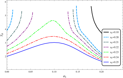
Figure 1: The time needed to form the apparent horizon of black hole with respect to different $a_{1}$. The lines from up to down denote $a_{2}=0.1,0.2,0.21,0.22,0.23,0.24,0.25$, respectively.

Different colors of lines indicate different strengths of the perturbation of the matter field $\psi$. We see that when the initial amplitude of the matter field perturbation is stronger, the time scale for the formation of the apparent horizon is shorter which means that the black hole can be formed more easily. This result is consistent with that observed in the Einstein gravity Gundlach_07 .

From the definition of the new scalar field $\phi$, we know that its strength indicates the deviation of the $f(R)$ gravity from the Einstein gravity. In the cosmological context, this new scalar field plays the role of inflaton or dark energy, acting as a repulsive force accounts for the accelerated expansion of the universe. When we fix the amplitude of the matter field perturbation $a_{2}$, we see that with the increase of the amplitude of the new scalar perturbation $a_{1}$, the repulsive effect brought in by the new scalar field dilutes the matter field perturbation and hinders the formation of the black hole so that it needs longer period of time for the apparent horizon to be developed. When the matter field perturbation is not strong enough, the increase of $a_{1}$ can even prevent the formation of the black hole through gravitational collapse. However when the amplitude of the new scalar perturbation $a_{1}$ is strong enough, we have observed some interesting results contrary to our naive understanding inherited from cosmology. Instead of prevention, the strong enough perturbation of the new scalar field can even stimulate the formation of black hole from gravitational collapse. The strong perturbation of the new scalar field (similar to the dark energy field) in comparable to the perturbation of the matter field does not exist in the cosmological scale. But it was discussed that the inhomogeneous perturbation of dark energy, although it is small, can contribute to the structure formation in cosmology Wang_10 aa . In the small scale, here we have seen that when the perturbation of the new scalar field is strong enough and is comparable to that of the matter field, it not only participates, but even stimulates the structure formation and makes the gravitational collapse quicker to form the black hole.

Dynamically, in addition to the kinetic energy of the matter field $\psi$ and the gravitational potential, the new scalar field $\phi$ adds a new competition force in the system. This is very similar to the study of the gravitational collapse of charged scalar field in our previous work Zhang_15 . We have seen that the dynamical competition can be controlled by tuning the parameters $a_{1}$ and $a_{2}$ in the initial perturbations of the new scalar field $\phi$ and the matter field $\psi$.

We want to emphasis that the phenomena we discovered are independent of the special types of initial conditions (26) we have chosen. We have checked that the numerical results hold with other kinds of initial conditions such as

$$\phi(0,r)=a_{1}\exp\left[-\left(\frac{r}{\sigma_{1}}\right)^{2}\right]r^{2} \psi(0,r)=a_{2}\exp\left[-\left(\frac{r}{\sigma_{2}}\right)^{2}\right]r^{2},$$ ,

$$\phi(0,r)=a_{1}\cos\left(\frac{\pi}{2}\tanh(r)\right) \psi(0,r)=a_{2}\cos\left(\frac{\pi}{2}\tanh(\frac{r}{2})\right),$$ , (30)

$$\phi(0,r)=a_{1}\cos\left(\frac{\pi}{2}\tanh(r)\right)r^{2} \psi(0,r)=a_{2}\cos\left(\frac{\pi}{2}\tanh(\frac{r}{2})\right)r^{2}.$$ ,

Similar qualitative results to Fig.1 have been discovered for different initial conditions. Thus the physical results we have obtained are universal.

In order to understand the phenomena in the above figure more clearly, we show the property of the gravitational potential in the following and examine how it evolves to trap the collapsing fields to form the black hole. Fixing the amplitude of the new scalar field perturbation $a_{1}$, the evolutions of the gravitational potential due to the change of the amplitude of matter field perturbation $a_{2}$ are shown in Fig.2.

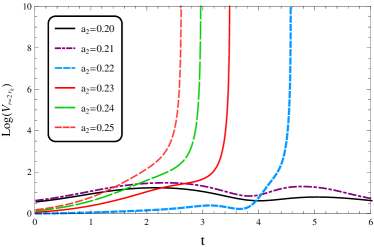
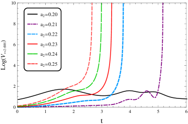
Figure 2: The evolution of the gravitational potential in the Einstein frame when $a_{1}=0.05$ (left) and $0.14$ (right), respectively.

It is easy to see that when the initial amplitude of the matter field perturbation is stronger, the gravitational potential grows up quicker so that the collapsing field is easier and quicker to be trapped in a small region to form a black hole.

In Fig.3 we fix the initial amplitude of the matter perturbation $a_{2}$ and exhibit the dependence of the evolution of the gravitational potential on the initial amplitude of the new scalar field perturbation $a_{1}$.

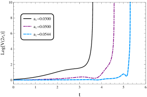
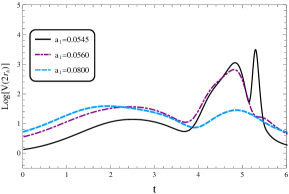
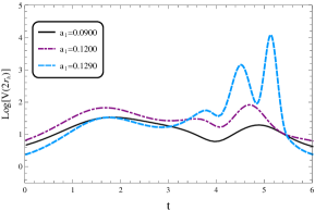
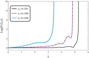
Figure 3: The time evolution of the gravitational potential at $r=2r_{h}$. We fix $a_{2}=0.22$ and let $a_{1}$ vary. Here $r_{h}$ is the apparent horizon of the black hole. If there are not black hole, $r_{h}$ is the position where $a(t,r)$ is minimum when the iteration stops.

In the upper left panel, we see that for the fixed amplitude of the matter field perturbation $a_{2}$, it takes longer time for the gravitational potential to grow when $a_{1}$ becomes bigger. This actually tells that more bounces of the matter field in the process of collapse are needed before the black hole formation. For $a_{1}=0.03$ the matter field needs two bounces and for $a_{1}=0.0544$ it needs four bounces to settle down to form black hole. In this panel the amplitude of the new scalar field perturbation $\phi$ is minor, thus although it plays the repulsive role, it cannot prevent the formation of the gravitational barrier to trap the matter field.

The upper right panel shows the gravitational potential behavior when $0.0545\leq a_{1}\leq 0.08$. We see that the gravitational potential is not strong enough to trap the matter field so that the matter field can run away instead of collapsing. The failure of forming a black hole is because of the strong repulsive force contributed by the new scalar field $\phi$. As $a_{1}$ increases, the peak of the gravitational potential becomes even smaller. The repulsion of the new scalar field $\phi$ now dominates the competition of dynamics.

In the lower left panel we exhibit the gravitational potential behavior when $0.09\leq a_{1}\leq 0.129$. Here something interesting happens. Though the repulsion of $\phi$ still wins the competition and gravitational potential is not strong enough to trap the matter field, the peak of gravitational potential becomes higher and higher as $a_{1}$ increases.

When $a_{1}>0.129$, the gravitational potentials are shown in the lower right panel. The gravitational potential becomes so big that black hole can be formed again. As $a_{1}$ increases, we see that the peak of the gravitational potential appears earlier and fewer bounces are needed for the matter field to settle down and being trapped to form the black hole. For example, there are four bounces of the matter field before the formation of black hole when $a_{1}=0.1291$. However, only two bounces are needed to form the black hole when $a_{1}=0.15$. The contribution of the strong perturbation in the small scale increases the gravitational binding effect so that the black hole formation through collapse becomes easier.

To be more instructive, we plot the the evolution of the Ricci scalar at $r=0$ in the Einstein frame for fixing $a_{1}$ first in Fig.4.

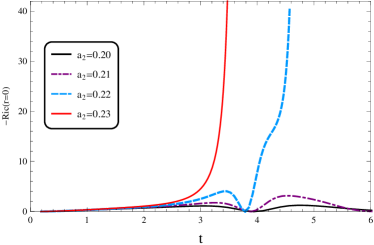
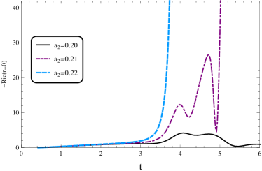
Figure 4: The evolution of the Ricci scalar in the Einstein frame at center $r=0$ when $a_{1}=0.05$ (left) and $0.14$ (right), respectively.

We see that for strong initial amplitude of the matter field perturbation $a_{2}$, the Ricci scalar diverges quicker at the center which indicates the black hole is more easily to be formed from the collapse.

Fixing the initial amplitude of the matter field perturbation $a_{2}=0.22$, the dependences of the Ricci scalar evolution on the initial amplitude of the new scalar field perturbation $a_{1}$ are shown in Fig.5.

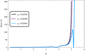
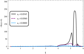
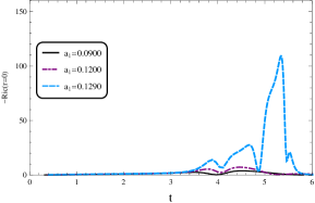
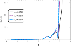
Figure 5: The evolution of Ricci scalar in the Einstein frame at center $r=0$ with respect to various $a_{1}$. We have fixed $a_{2}=0.22$.

We see that at the center the Ricci scalar in the Einstein frame tends to diverge when the black hole can be formed, while converge when the collapsing field is dispersed. The influence of the $a_{1}$ on the time scale for the blow up of the Ricci curvature is consistent with that in the gravitational potential in Fig.3. Actually this gives us further understanding on the different influences of the new scalar field and the matter field in the formation of black hole through the gravitational collapse.

V Conclusions and discussions

In this paper we have studied the gravitational collapse in the model of a spherically symmetric, massless scalar field $\psi$, minimally coupled to gravity in a specific $R^{2}$ model in $f(R)$ gravity. Adopting the usual treatment, we have done the conformal transformation and expressed the $f(R)$ gravity in the Einstein frame. The conformal transformation from Jordan frame to Einstein frame brought a new scalar field to the system which is coupled to the matter field. In the cosmological context this new scalar field plays the role of the repulsive force just like the inflaton or dark energy in the early or late time accelerated expansion of the universe. On the other hand, this field can also work as dark matter Cembranos:2008gj ; Cembranos:2010qd . Thus at the first sight, the black hole formation through gravitational collapse in the $f(R)$ gravity contains more competitions between repulsive and attractive effects in dynamics than that in the Einstein general gravity.

Our numerical calculation focused on the Starobinsky $R^{2}$ gravity model, which can account for the inflation in the early universe. Adopting the Choptuik’s formalism, we have studied the evolution of the dynamical system satisfying the matter-gravity equations. We have found that the formation of the black hole from the gravitational collapse depends on the thresholds of initial amplitudes of perturbations in the new scalar field introduced from conformal transformation and in the original matter field perturbation. Fixing the newly scalar field introduced by conformal transformation, we found that when the amplitude of the initial matter field perturbation is strong, the black hole can be formed more easily and more quickly. When we fix the amplitude of the initial matter perturbation field, with the increase of the amplitude of the initial scalar perturbation brought by the conformal transformation in the Einstein frame, the formation of the black hole from the gravitational collapse is hindered at first due to the repulsive effect of this new scalar field. If the matter perturbation is weak, the repulsive effect of the new scalar field can even prevent the formation of the black hole. However when the initial perturbation of the scalar field can be comparable to that of the matter field, when we increase further the initial amplitude of the scalar perturbation, we have observed that this new scalar perturbation can participate the structure formation in the gravitational collapse and stimulates the black hole formation. This result in the small scale gravitational collapse is different from our usual understanding from the cosmological context in the large scale.

We have examined carefully the competitions in dynamics by investigating the gravitational potential in the system which plays the major role to trap the collapsing fields and contributes to the black hole formation. It is interesting that we have clearly shown that the dynamical competition can be controlled by tuning the parameters in the initial perturbations in the new scalar field and the matter field. To show the result more instructive, we have also calculated the Ricci scalar at the center and its dependence of the tuning of parameters in the initial perturbations. These results can help us understand better the gravitational collapse in the $f(R)$ gravity.

We have transformed the results back to the Jordan frame from that we obtained in the Einstein frame. We see that the location of the horizon in the Jordan frame is the same as that in the Einstein frame since the conformal factor is regular at the horizon. Considering that the standard matter are minimally coupled to the metric in the Jordan Frame, it would be very interesting to know how the collapse process looks in the Jordan frame. But direct computation in the Jordan frame is difficult as we discussed, since we can not specify natural high order boundary conditions from physics to solve the fourth order differential equations. It was argued that Jordan frame and Einstein frame are equivalent, especially in the cosmological context He2012 ; Domenech2016 ; Chiba2013 , which implies that the properties of gravitational collapse we obtained in the Einstein frame also should hold in the Jordan frame. The relation between the Einstein frame and Jordan frame was also discussed in Sotiriou_08 ; Felice_10 . To disclose exactly how the gravitational collapse happens in the Jordan frame, careful investigation is still called for.

References

- (1) D. Christodoulou, A Mathematical Theory of Gravitational Collapse, Commun. Math. Phys. 109, 613 (1987).
- (2) D. Christodoulou, The formation of black holes and singularities in spherically symmetric gravitational collapse, Commun. Pure Appl. Math. 44, no. 3, 339 (1991).
- (3) D. Christodoulou, Examples of naked singularity formation in the gravitational collapse of a scalar field, Annals Math. 140, 607 (1994).
- (4) R. M. Wald, Gravitational collapse and cosmic censorship, In *Iyer, B.R. (ed.) et al.: Black holes, gravitational radiation and the universe* 69-85, gr-qc/9710068.
- (5) M.W. Choptuik, Critical behavior in massless scalar field collapse, in d’Inverno, R., ed., Approaches to Numerical Relativity, Proceedings of the International Workshop on Numerical Relativity, Southampton, December 1991, 202, (Cambridge University Press, Cambridge, U.K.; New York, U.S.A., 1992).
- (6) M.W. Choptuik, Universality and scaling in gravitational collapse of a massless scalar field, Phys. Rev. Lett., 70(1), 9-12, (1993).
- (7) M.W. Choptuik, Critical behavior in scalar field collapse, in Hobill, D., Burd, A., and Coley, A., eds., Deterministic Chaos in General Relativity, Proceedings of a NATO Advanced Research Workshop on Deterministic Chaos in General Relativity, held July 25-30, 1993, in Kananaskis, Alberta, Canada, 155, (Plenum Press, New York, U.S.A., 1994).
- (8) M.W. Choptuik, The (Unstable) threshold of black hole formation, arXiv:gr-qc/9803075.
- (9) A. Wang, Critical phenomena in gravitational collapse: The Studies so far, Braz.J.Phys. 31 (2001) 188-197, arXiv:gr-qc/0104073.
- (10) C. Gundlach, J. M. Martin-Garcia, Critical phenomena in gravitational collapse, Living Rev.Rel. 10 (2007) 5, arXiv:0711.4620 [gr-qc].
- (11) S. Hod, T. Piran, Critical behavior and universality in gravitational collapse of a charged scalar field, Phys.Rev. D55 (1997) 3485-3496, arXiv: gr-qc/9606093.
- (12) Y. Iwashita, H. Yoshino, T. Shiromizu, Gravitational collapse disturbs the dS/CFT correspondence? Phys.Rev. D72 (2005) 084014, gr-qc/0507076.
- (13) C.-Y. Zhang, S.-J. Zhang, D.-C. Zou, B. Wang, Charged scalar gravitational collapse in de Sitter spacetime, Phys. Rev. D 93, 064036 (2016), arXiv:1512.06472 [gr-qc].
- (14) P. Bizoń, A. Rostworowski, On weakly turbulent instability of anti-de Sitter space, Phys.Rev.Lett.107:031102,2011, arXiv:1104.3702 [gr-qc].
- (15) D. Garfinkle, L. A. Pando Zayas, D. Reichmann, On Field Theory Thermalization from Gravitational Collapse, JHEP 1202 (2012) 119, arXiv:1110.5823 [hep-th].
- (16) O. J. C. Dias, G. T. Horowitz, J. E. Santos, Gravitational Turbulent Instability of Anti-de Sitter Space, Class.Quant.Grav. 29 (2012) 194002, arXiv:1109.1825 [hep-th].
- (17) S. L. Liebling, C. Palenzuela, Dynamical Boson Stars, Living Rev.Rel. 15 (2012) 6, arXiv:1202.5809 [gr-qc].
- (18) B. Wu, On holographic thermalization and gravitational collapse of massless scalar fields, JHEP 1210 (2012) 133, arXiv:1208.1393 [hep-th].
- (19) M. Maliborski, Instability of Flat Space Enclosed in a Cavity, Phys.Rev.Lett. 109 (2012) 221101, arXiv:1208.2934 [gr-qc].
- (20) A. Buchel, L. Lehner, S. L. Liebling, Scalar Collapse in AdS, Phys.Rev. D86 (2012) 123011, arXiv:1210.0890 [gr-qc].
- (21) M. Maliborski, A. Rostworowski, Time-Periodic Solutions in an Einstein AdS-Massless-Scalar-Field System, Phys.Rev.Lett. 111 (2013) 051102, arXiv:1303.3186 [gr-qc].
- (22) B. Craps, . Evnin, J. Vanhoof, Renormalization group, secular term resummation and AdS (in)stability, JHEP 1410 (2014) 048, arXiv:1407.6273 [gr-qc].
- (23) V. Balasubramanian, A. Buchel, S. R. Green, L. Lehner, Steven L. Liebling, Holographic Thermalization, Stability of Anti-de Sitter Space, and the Fermi-Pasta-Ulam Paradox, Phys.Rev.Lett. 113 (2014) no.7, 071601, arXiv:1403.6471 [hep-th].
- (24) R.-G. Cai, L.-W. Ji, R.-Q. Yang, Collapse of self-interacting scalar field in anti-de Sitter space, Commun.Theor.Phys. 65 (2016) no.3, 329-334, arXiv:1511.00868 [gr-qc].
-
(25)
R.-G. Cai, R.-Q. Yang, Scaling Laws in Gravitational
Collapse, arXiv:1512.07095 [gr-qc].
R.-G. Cai, R.-Q. Yang, Multiple critical gravitational collapse of charged scalar with reflecting wall, arXiv:1602.00112 [gr-qc].
Z. Cao, R.-G. Cai, R.-Q. Yang, Multi-horizon and Critical Behavior in Gravitational Collapse of Massless Scalar, arXiv:1604.03363 [gr-qc]. - (26) N. Deppe, A. Kolly, A. Frey, G. Kunstatter, Stability of AdS in Einstein Gauss Bonnet Gravity, Phys.Rev.Lett. 114 (2015) 071102, arXiv:1410.1869 [hep-th].
- (27) S. L. Liebling, M. W. Choptuik, Black Hole Criticality in the Brans-Dicke Model, Phys.Rev.Lett. 77 (1996) 1424-1427, arXiv:gr-qc/9606057.
- (28) T. Chiba, J. Soda, Critical Behavior in the Brans-Dicke Theory of Gravitation, Prog.Theor.Phys. 96 (1996) 567-574, arXiv:gr-qc/9603056.
- (29) G. Koutsoumbas, K. Ntrekis, E. Papantonopoulos, M. Tsoukalas, Gravitational Collapse in Horndeski Theory, arXiv:1512.05934 [gr-qc].
- (30) P. Cañate, L. G. Jaime, M. Salgado, Spherically symmetric black holes in gravity: Is geometric scalar hair supported? arXiv:1509.01664 [gr-qc].
- (31) A. A. Starobinsky, A New Type of Isotropic Cosmological Models Without Singularity , Phys.Lett. B91 (1980) 99-102
- (32) S. M. Carroll, V. Duvvuri, M. Trodden, M. S. Turner, Is Cosmic Speed-Up Due to New Gravitational Physics?, Phys.Rev.D70:043528,2004, arXiv:astro-ph/0306438.
- (33) M. Sharif, H. R. Kausar, Gravitational Perfect Fluid Collapse in f(R) Gravity, Astrophys. Space Sci.331:281-288, 2011, arXiv:1007.2852 [gr-qc].
- (34) M. Sharif, Z. Yousaf, Dynamical instability of the charged expansion-free spherical collapse in f(R) gravity, Phys.Rev. D88 (2013) 024020.
- (35) M. Sharif, Z. Yousaf, Stability analysis of cylindrically symmetric self-gravitating systems in gravity, Mon.Not.Roy.Astron.Soc. 440 (2014) no.4, 3479-3490.
- (36) H. R. Kausar, I. Noureen, Dissipative Spherical Collapse of Charged Anisotropic Fluid in f(R) Gravity, Eur.Phys.J. C74 (2014) no.99, 2760, arXiv:1401.8085 [gr-qc].
- (37) S. Chakrabarti, N. Banerjee, Spherically symmetric collapse of a perfect fluid in f(R) gravity, Gen.Rel.Grav. 48 (2016) no.5, 57 , arXiv:1603.08629 [gr-qc].
- (38) D.-i. Hwang, B.-H. Lee, D.-h. Yeom, Mass inflation in f(R) gravity: A Conjecture on the resolution of the mass inflation singularity, J. Cosmol. Astropart. Phys. 1112, 006 (2011). arXiv:1110.0928 [gr-qc].
- (39) J. A. R. Cembranos, A. de la Cruz-Dombriz, B. Montes Nuñez, Gravitational collapse in f(R) theories, JCAP 1204 (2012) 021, arXiv:1201.1289 [gr-qc].
- (40) M. Kopp, S. A. Appleby, I. Achitouv, J. Weller, Spherical collapse and halo mass function in theories, Phys. Rev. D 88, 084015 (2013), arXiv:1306.3233 [astro-ph.CO].
- (41) J.-Q. Guo, D. Wang, A. V. Frolov, Spherical collapse in f(R) gravity and the Belinskii-Khalatnikov-Lifshitz conjecture, Phys. Rev. D 90, 024017 (2014), arXiv:1312.4625 [gr-qc].
- (42) R. Goswami, A. M. Nzioki, S. D. Maharaj, S. G. Ghosh, Collapsing spherical stars in gravity, Phys. Rev. D 90, 084011 (2014), arXiv:1409.2371 [gr-qc].
- (43) J.-Q. Guo, P. S. Joshi, Spherical collapse for the Starobinsky model, arXiv:1511.06161 [gr-qc].
- (44) T. P. Sotiriou, V. Faraoni, f(R) Theories Of Gravity, Rev. Mod. Phys. 82:451-497,2010, arXiv:0805.1726 [gr-qc].
- (45) A. D. Felice, S. Tsujikawa, f(R) theories, Living Rev. Rel. 13: 3, 2010, arXiv:1002.4928 [gr-qc].
- (46) J. A. R. Cembranos, Dark Matter from R2-gravity,, Phys. Rev. Lett. 102, 141301 (2009), arXiv:0809.1653 [hep-ph].
- (47) J. A. R. Cembranos, Dark Matter, J. Phys. Conf. Ser. 315, 012004 (2011), arXiv:1011.0185 [gr-qc].
- (48) B. Wang, E. Abdalla, F. Atrio-Barandela, D. Pavon, Dark Matter and Dark Energy Interactions: Theoretical Challenges, Cosmological Implications and Observational Signatures, Reports on Progress in Physics, Volume 79, Number 9, arXiv:1603.08299 [astro-ph.CO].
- (49) A. Vilenkin, Classical and Quantum Cosmology of the Starobinsky Inflationary Model, Phys.Rev. D32 (1985) 2511.
- (50) M. Maliborski and A. Rostworowski, Lecture Notes on Turbulent Instability of Anti-de Sitter Spacetime, Int. J. Mod. Phys. A 28, 1340020 (2013), arXiv:1308.1235 [gr-qc].
- (51) H.-O. Kreiss and J. Oliger, Comparison of accurate methods for the integration of hyperbolic equations, Tellus 24 (1972) no. 3, 199-215.
- (52) J.-H. He, B. Wang, E. Abdalla, D. Pavon, The imprint of the interaction between dark sectors in galaxy clusters, JCAP 1012:022,2010, arXiv:1001.0079 [gr-qc].
- (53) P. Creminelli, G. D’Amico, J. Norena, L. Senatore, and F. Vernizzi, Spherical collapse in quintessence models with zero speed of sound, JCAP 03, 027 (2010), arXiv:0911.2701.
- (54) J.-H. He, B. Wang, Modeling gravity in terms of mass dilation rate, arXiv:1203.2766 [astro-ph.CO].
- (55) G. Domenech, M. Sasaki, Conformal frames in cosmology, arXiv:1602.06332 [gr-qc].
- (56) T. Chiba, M. Yamaguchi, Conformal-Frame (In)dependence of Cosmological Observations in Scalar-Tensor Theory, JCAP 1310:040,2013, arXiv:1308.1142 [gr-qc].