Long-range transverse Ising model built with dipolar condensates in two-well arrays

Abstract

Dipolar Bose-Einstein condensates in an array of double-well potentials realize an effective transverse Ising model with peculiar inter-layer interactions, that may result under proper conditions in an anomalous first-order ferromagnetic-antiferromagnetic phase transition, and nontrivial phases due to frustration. The considered setup allows as well for the study of Kibble-Zurek defect formation, whose kink statistics follows that expected from the universality class of the mean-field one-dimensional transverse Ising model. Furthermore, random occupation of each layer of the stack leads to random effective Ising interactions and local transverse fields, that may lead to the Anderson-like localization of imbalance perturbations.

Key-words: Dipole-dipole interactions, Long-range Ising model, Kibble-Zurek scenario, Anderson localization.

I Introduction

A new generation of experiments with ultra-cold magnetic atoms Griesmaier2005 ; Lu2011 ; Aikawa2012 ; DePaz2013 , polar molecules Ni2008 ; Yan2013 ; Takehoshi2014 ; Park2015 , and Rydberg-dressed atoms Rydberg-Dressed are starting to reveal novel fascinating physics of dipolar gases. Whereas in non-dipolar Bose gases inter-particle interactions are short-range and isotropic, dipolar gases present significant or even dominant dipole-dipole interactions (DDI), which are long-range and anisotropic. As a result, the physics of dipolar gases strongly differs from that of their non-dipolar counterparts Lahaye2009 ; Baranov2012 , featuring effects such as geometry-dependent stability Koch2008 , roton-like excitations Santos2003 ; Wilson2008 and roton-dominated immiscibility immiscibility ; Young2012 , strongly anisotropic vortices vortex ; YiS2006 ; Abad2009 and solitons soliton1 ; soliton2 , ferrofluidity ferrofluidity ; Saito2009 and anisotropic superfluidity Bohn , striped patterns stripes , specific mesoscopic configurations trapped in triple potential wells triple , double- and triple-periodic ground states in lattices populated by dipolar atoms Tilman , and the recent discovery of robust quantum droplets Kadau2016 ; Ferrier2016 .

Dipolar gases in optical lattices are also remarkably different from their non-dipolar counterparts Lahaye2009 ; Baranov2012 . Whereas in the absence of DDI, interparticle interactions in deep lattices reduce to on-site nonlinearity, the DDI result in inter-site interactions. The latter is true even for very strong lattices, in which inter-site tunneling vanishes. As a result, dipolar lattice gases allow for the transport of excitations in the absence of mass transfer. Recently, spin-like transport was studied in gases of magnetic atoms DePaz2013 and polar molecules Yan2013 , where the spin was encoded, respectively, in the electronic spin and in the rotational degree of freedom. The dipole-induced spin exchange and Ising interactions result in an effective XXZ Hamiltonian Micheli2006 ; Gorshov2011 . It has been recently shown that in an imperfectly filled lattice the dipole-induced spin exchange may result in a peculiar disorder scenario Deng2016 .

In this paper, we discuss a set-up that permits for coding spin-like systems into a spatial degree of freedom of a dipolar Bose-Einstein condensate (BEC). The condensate is prepared in a stack of layers of two-well potentials that emulate an effective spin-$1/2$ system (see Fig. 1). This set-up realizes a transverse Ising model with a peculiar form of long-range interactions that results in an unconventional first-order ferromagnetic-antiferromagnetic transition, as well as in phases with anomalous periodicities due to magnetic frustration. Since the parameters may be easily changed in real-time the model allows as well for quenching through second-order phase transitions, as we illustrate for the particular case of a transition from an effective paramagnet into a ferromagnet. We show that the associated defect formation follows the Kibble-Zurek (KZ) Kibble1980 ; Zurek1996 ; Dziarmaga scaling expected from the universality class of the mean-field one-dimensional transverse Ising model. Furthermore, we show that random layer filling results in an effective disorder in both the Ising-like interactions and the local transverse field, allowing for the observation of Anderson-like localization of imbalance perturbations.

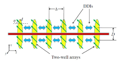
Figure 1: (Color online) Sketch of the setup considered: a stack of two-well arrays of dipolar condensates formed an effective one-dimensional transverse Ising model.

The paper is organized as follows. In Sec. II we introduce the set-up and derive the effective long-range transverse Ising model. Section III discusses the corresponding ground-state phases, whereas Sec. IV comments on the formation of KZ defects. Section V discusses the effective disorder resulting from random layer filling and the associated Anderson-localization in the imbalance transport. Finally Sec. VI summarizes our conclusions.

II The model

We consider in the following a stack of axisymmetric quasi-one-dimensional dipolar BECs (“wires”), separated along the $z$ direction by a distance $\Delta$, with their axes oriented along $x$, as shown in Fig. 1. This configuration may be readily created by loading the BEC into just one plane of a 2D optical lattice created in the $yz$ plane. The lattice is assumed deep enough, to suppress both on-site dynamics along the $y$ and $z$ directions and tunneling between adjacent condensates. An additional double-well potential $U(x)$, with inter-well spacing $D$, is placed along the $x$ axis, while the atomic dipole moments are parallel to the $xz$ plane, forming angle $\eta$ with the $z$ axis. The system is described by a set of coupled one-dimensional Gross-Pitaevskii (GP) equations:

$$i\hbar\frac{\partial}{\partial t}\psi_{n}(x,t)=\left[-\frac{\hbar^{2}}{2m}\frac{\partial^{2}}{\partial x^{2}}+U(x)+\mathcal{V}_{n}(x)\right]\psi_{n}(x,t),$$ (1)

with $m$ the particle mass, $\psi_{n}(x,t)$ the axial wave function at site $n$, and

$$\mathcal{V}_{n}(x)\equiv\int_{-\infty}^{+\infty}dx^{\prime}\left[\sum_{n^{\prime}}V_{n^{\prime}-n}(x-x^{\prime})+g_{1D}\delta(x-x^{\prime})\delta_{n^{\prime}n}\right]|\psi_{n^{\prime}}(x^{\prime},t)|^{2}.$$ (2)

The contact interactions are characterized by $g_{1D}=\frac{2\hbar^{2}a}{ml^{2}}$, with $a$ the scattering length, and $l$ the effective oscillator length associated to the on-site confinement in the $yz$ plane. $V_{n^{\prime}-n}(x)$ is the DDI between dipoles placed $n^{\prime}-n$ sites apart and separated by an axial distance $x$. The kernel $V_{n^{\prime}-n}(x)$ is the Fourier transform of

$$\tilde{V}_{n^{\prime}-n}(k_{x})=\int\frac{dk_{y}}{2\pi}\int\frac{dk_{z}}{2\pi}\tilde{V}_{\mathrm{dd}}(\vec{k})e^{-ik_{z}(n^{\prime}-n)\Delta}e^{-(k_{y}^{2}+k_{z}^{2})l^{2}/2},$$ (3)

with $\tilde{V}_{\mathrm{dd}}(\vec{k})=\frac{4\pi}{3}d^{2}\left[3|\vec{k}|^{-2}(k_{z}\cos\eta+k_{x}\sin\eta)^{2}-1\right]$ and $d$ the dipole moment.

For a sufficiently tight $U(x)$ potential, we may employ a simplified two-mode scenario in which only the two lowest eigenstates of $U(x)$ participate in the dynamics, $(R(x)\pm L(x))/\sqrt{2}$, where $R(x)$ ($L(x)$) denote the wave functions at the right (left) well. We may then express $\psi_{n}(x,t)=a_{n}(t)L(x)+b_{n}(t)R(x)$. The two wells are coherently coupled by a hopping rate $J$ footnote-quantum . Under these conditions, the coupled GP equations (1) reduce to

$$i\dot{a}_{n}(t) = -Jb_{n}(t)+\tilde{\mu}_{n}(t)a_{n}(t),$$ (4)

$$i\dot{b}_{n}(t) = -Ja_{n}(t)+\tilde{\mu}_{n}^{\prime}(t)b_{n}(t),$$ (5)

where

$$\tilde{\mu}_{n}(t) \equiv \sum_{n^{\prime}}\left[\left(\tilde{F}_{0}\left(n^{\prime}-n\right)+U_{0}\delta_{n^{\prime}n}\right)\left|a_{n^{\prime}}(t)\right|^{2}\right.$$ (6)

$$\left.+\tilde{F}_{0}\left(n^{\prime}-n\right)\left|b_{n^{\prime}}(t)\right|^{2}\right]N_{n^{\prime}},$$

$\tilde{\mu}^{\prime}$ is defined with $a_{n}\rightleftarrows b_{n}$, $U_{0}\equiv g_{1D}\int_{-\infty}^{+\infty}dx|R(x)|^{4}$, $\tilde{F}_{0}(n^{\prime}-n)\equiv\int_{-\infty}^{+\infty}dx\int_{-\infty}^{+\infty}dx^{\prime}V_{n^{\prime}-n}(x-x^{\prime})|R(x)|^{2}|R(x^{\prime})|^{2}$ denotes the interaction between right wells at two sites placed $n\Delta$ apart (or equivalently between left wells), $\tilde{F}_{1}(n^{\prime}-n)\equiv\int_{-\infty}^{+\infty}dx\int_{-\infty}^{+\infty}dx^{\prime}V_{n^{\prime}-n}(x-x^{\prime})|A(x)|^{2}|B(x^{\prime})|^{2}$ is the interaction between left and right wells, and $N_{n}$ denotes the number of particles in the $n$-th wire. Since we assume a vanishing inter-site hopping, $N_{n}$ is conserved, and $|a_{n}|^{2}+|b_{n}|^{2}=1$. In the following, we assume that the scattering length is tuned by means of Feshbach resonances, so that $U_{0}=\tilde{F}_{1}(0)-\tilde{F}_{0}(0)$. In this way, the on-site (dipolar plus contact) interactions cancel, allowing us to concentrate on the non-trivial dynamics arising from the inter-layer DDI. Finally, although the exact form of $\tilde{F}_{0}(n^{\prime}-n)$ and $\tilde{F}_{1}(n^{\prime}-n)$ may be evaluated exactly, we may further simplify the model by considering a point-like approximation that yields

$$\frac{F_{0}(n^{\prime}-n)}{d^{2}/\Delta^{3}}=\frac{1-3\cos^{2}\eta}{(n^{\prime}-n)^{3}},$$

$$\frac{F_{1}(n^{\prime}-n)}{d^{2}/\Delta^{3}}=\frac{1}{\left[(n^{\prime}-n)^{2}+\left(D/\Delta\right)^{2}\right]^{3/2}}$$

$$-\frac{3\left[(n^{\prime}-n)\cos\eta+\left(D/\Delta\right)\sin\eta\right]^{2}}{\left[(n^{\prime}-n)^{2}+\left(D/\Delta\right)^{2}\right]^{5/2}}.$$ (7)

The exact evaluation of $F_{0}$ and $F_{1}$ may modify these values, especially for nearest-neighboring wires for which the finite wave packet spreading may be significant compared to the inter-site spacing, but our results would remain qualitatively unaffected.

III Ground-state phases

Interestingly, the system under consideration is equivalent to a spin-$1/2$ transverse Ising model with peculiar long-range Ising interactions given by the Hamiltonian

$$H=-J\sum_{n}N_{n}S^{x}_{n}+{1\over 2}\sum_{n,n^{\prime}}N_{n}N_{n^{\prime}}V_{S}(n-n^{\prime})S^{z}_{n}S^{z}_{n^{\prime}},$$ (8)

where $-J$ plays the role of an effective transversal magnetic field, $V_{S}(n^{\prime}-n)\equiv\left[F_{0}(n^{\prime}-n)-F_{1}(n^{\prime}-n)\right]/2$ characterizes an effective Ising-like coupling, and we have introduced the effective spin components $S^{x}_{n}=a^{\ast}_{n}b_{n}+\mathrm{c.c}$ and $S^{z}_{n}=|b_{n}|^{2}-|a_{n}|^{2}$.

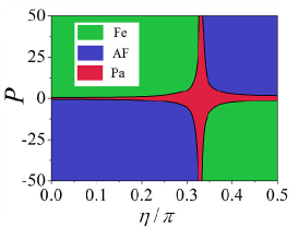
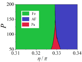
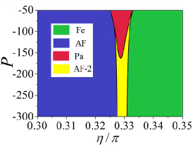
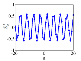
Figure 2: (Color online) (a) Ground-state phase diagram as a function of the DDI strength $P=Nd^{2}/J\Delta^{3}$ and the angle $\eta$. (b) Vicinity of $\eta_{\mathrm{cr}}$ for $P>0$, showing the first-order F-AF transition. (c) Vicinity of $\eta_{\mathrm{cr}}$ for $P<0$, showing the appearance of the AF-2 phase. (d) AF-2 phase for $\eta=\eta_{\mathrm{cr}}$ and $P=-180$; note the formation of an AF order with a periodicity of approximately five wires.

At this point, we assume that all layers are equally populated, $N_{n}\equiv N$ (we relax this condition in Sec. V). We fix the hopping rate as the energy unit, i.e. $J=1$, and also set $D=1$. The strength of the DDI is characterized by the parameter $P=Nd^{2}/J\Delta^{3}$, which plays a key role in the discussion below. For the particular case of dysprosium atoms with an inter-wire separation of $\Delta=1\mu$m, $d^{2}/\Delta^{3}\sim 1$ Hz, and hence for $N=10^{3}$–$10^{4}$ atoms, $Nd^{2}/\Delta^{3}=1$–$10$ kHz. The corresponding value of $P$ depends on $J$, which is controlled by the barrier of the two-well potential $U(x)$. For typical values $J\sim 100$ Hz, $P\sim 100$ may be hence readily reached.

The ground-state phase diagram of the system footnote-quantum , presented in Fig. 2, is obtained numerically from the imaginary-time evolution of Eqs. (4) and (5). If $\eta$ is such that $V_{S}(n^{\prime}-n)<0$, the Ising interaction is ferromagnetic. For $P/J=0$ the ground-state of the system is given by a spin oriented along the transversal magnetic field, i.e., along $x$-axis, and hence a solution with zero imbalance $S^{z}_{n}=0$ is favored. This ground state corresponds to the paramagnetic (Pa) phase. For a sufficiently large $P>P_{\mathrm{cr}}$ ($P_{\mathrm{cr}}\simeq 0.45J$ for $\eta=0$), the system experiences a second-order phase transition into a ferromagnetic (F) phase, characterized by a full imbalance, either to the $R$ or to the $L$ well. At $\eta_{\mathrm{cr}}\approx 0.33\pi$, $V_{S}(1)=0$ and hence the nearest-neighbor (NN) interaction changes the sign. As a result for $\eta>\eta_{\mathrm{cr}}$ at a sufficiently large $P/J$ the system enters an Ising anti-ferromagnetic (AF) phase, characterized by a staggered imbalance between neighboring wires. The situation is obviously reversed for $P<0$ (which may be achieved by means of a rotating magnetic field Giovanazzi2002 ), and the Pa-AF transition occurs for $\eta<\eta_{\mathrm{cr}}$ and Pa-F for $\eta>\eta_{\mathrm{cr}}$.

The situation is particularly noteworthy in the vicinity of $\eta_{\mathrm{cr}}$. Whereas for $P<P_{\mathrm{cr}}(\eta_{\mathrm{cr}})\approx 147$, the F and AF phases remain separated by a Pa phase, for $P>P_{\mathrm{cr}}(\eta_{\mathrm{cr}})$ there is a first-order F-AF phase transition, see Fig. 2(b). The reason for this change is that, when $|V_{S}(1)|<|V_{S}(2)|$ at $\eta=\eta_{\mathrm{cr}}$, $V_{S}(2)$ remains negative, i.e., $V_{S}(2)$ favors ferromagnetism between next-nearest-neighbors (NNN). This is both compatible with Néel ordering and with a fully ferromagnetic state. The only difference between these two choices is the orientation between NN, which steeply changes when $V_{S}(1)$ changes its sign. This is remarkably different from the usual situation in NN Ising models, with $V_{S}(n>1)=0$, in which the change of the sign of $V_{S}(1)$ implies vanishing interactions, and hence the Pa phase always separates the F and AF phases. It is also different from the standard version of the long-range transverse Ising model induced by dipolar interactions, i.e., $V_{S}(n^{\prime}-n)=V_{0}/(n^{\prime}-n)^{3}$. In that case, the change of the NN coupling at $V_{0}=0$ from F to AF also implies vanishing of all interactions, and hence the existence of an intermediate Pa phase. Here, when $P>P_{\mathrm{cr}}(\eta_{\mathrm{cr}})$, $V_{S}(1)$ is negligible, and $V_{S}(2)$ dominates. Such a dominating ferromagnetic NNN coupling allows for a direct first-order transition between F and AF as a function of $\eta$.

A similar competition at $P<0$ results in magnetic frustration. In the vicinity of $\eta_{\mathrm{cr}}$, when $|V_{S}(1)|<|V_{S}(2)|$, one has $V_{S}(2)>0$. Under these conditions, the system experiences frustration, as AF NNN interactions are now incompatible with the small F or AF NN coupling. As a result, in the vicinity of $\eta_{\mathrm{cr}}$, a new phase (AF-2) develops, see Fig. 2(c), with an approximate five-site-periodic modulation of the imbalance, see Fig. 2(d).

IV Kibble-Zurek scenario

As shown in Sec. III varying $P$ and/or $\eta$ permits accessing various second-order phase transitions. We note that both parameters may be modified in real time. In particular $P$ may be readily modified by altering the barrier between the two wells, since the latter controls the value of $J$. This provides the possibility of quenching in real time through the second-order phase transitions of Fig. 2. Quenching at a finite speed is expected to induce defects due to the Kibble-Zurek (KZ) mechanism Kibble1980 ; Zurek1996 ; Dziarmaga .

We illustrate this possibility with the particular case of the Pa-F transition. Increasing $P$ for $\eta=0$ eventually quenches from the fully balanced Pa phase into the F one. As a result, the system develops F domains, i.e. regions with total imbalance biased to the $R$ or $L$ sites, separated by a domain wall (kink). In our simulations of Eqs. (4) and (5), we consider a balanced input with a slight random imbalance and relative phase perturbation: $a_{n}=(0.5-\varepsilon\,\mathrm{\rho}_{1})^{1/2}\,\exp(i\varepsilon\,\mathrm{\rho}_{2})$ and $b_{n}=(0.5+\varepsilon\,\mathrm{\rho}_{1})^{1/2}\,\exp(-i\varepsilon\,\mathrm{\rho}_{2})$, where $-1<\mathrm{\rho}_{1,2}<1$ are two sets of random numbers, and $\varepsilon\ll 1$ ($10^{-6}$ in our calculations) is the strength of the randomness. This small randomness mimics slight imperfections that seed the domain-wall formation. We then impose a linear ramp, $P(t)=\gamma t$, with different ramp speeds $\gamma$. Typical numerical results for two values of $\gamma$ are displayed in Figs. 3(a) and (b). As expected, the number of kinks increases with the ramp speed $\gamma$ when crossing the transition. From a large number of random realizations (up to $50$ different sets of $\rho_{1,2}$), we extract, for each value of $\gamma$, statistics of the number of the domain walls, $N_{D}$. Figure 3 (c) depicts $\ln(N_{D})$ as a function of $\ln(\gamma)$, showing that $N_{D}\sim\gamma^{1/2}$. The later follows the known KZ scaling, $N_{\mathrm{D}}\sim\gamma^{\nu/(\nu z+1)}$, where $\nu=1$ and $z=1$ are the critical static and dynamical exponents for the mean-field one-dimensional transverse Ising model Dziarmaga .

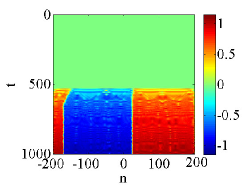
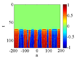
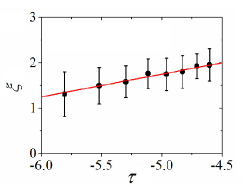
Figure 3: (Color online) Pattern formation in the imbalance distribution as a function of time for $\eta=0$ and a linear ramp $P(t)=\gamma t$ with a ramp speed $\gamma=10^{-3}$ (a) and $10^{-2}$ (b); (c) $\xi=\ln N_{\mathrm{D}}$, where $N_{\mathrm{D}}$ is the number of domains, as a function of $\tau\equiv\ln\gamma$, the results being best fitted by $\xi=4.25+0.5\tau$, which implies that $N_{\mathrm{D}}\propto\gamma^{1/2}$, as expected from the KZ scaling.

V Imbalance transport in the presence of random fillings

The coupling between layers in Eq. (8) crucially depends on the number of particles in each layer. This opens interesting possibilities for the study of excitation transport — in particular, localization due to random interactions, rather than due to random hopping (we recall that mass transport between wires is suppressed). We consider a randomized distribution of the number of particles in each wire, $N_{n}/N=1+\varepsilon R_{n}$, where $-1<R_{n}<1$ are random numbers, and $\varepsilon\in[0,1]$ determines the strength of the randomness. Such random distributions may be created by abruptly growing the lattice on top of a trapped BEC. Note that the random population in each wire translates into a random inter-wire interaction in Eq. (8), which may significantly affect the transport of imbalanced excitations.

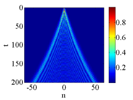
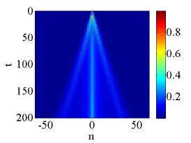
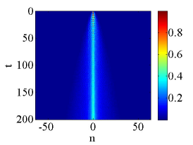
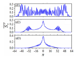
Figure 4: (Color online) Averaged imbalance distribution $\overline{S_{j}^{z}}(t)$ for an initial imbalance perturbation localized at the site $n=0$, with $\eta=0$, $P=0.1$, and a disorder strength (see text) $\varepsilon=0$ (a), $0.4$ (b), and $0.8$ (c). Figure (d) shows from top to bottom $\overline{S_{n}^{z}}(t=200)$ for $\varepsilon=0$, $0.4$, and $0.8$.

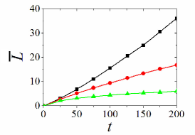
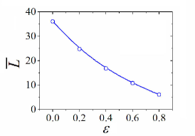
Figure 5: (Color online) For the same case of Fig. 4: (a) width $\overline{L}(t)$ for $\varepsilon=0$ (black squares), $0.4$ (red circles) and $0.8$ (green triangles); (b) $\overline{L}(t=200)$ as a function of the disorder strength $\varepsilon$.

We here consider an initially localized imbalance excitation on top of an otherwise perfectly balanced system, i.e., $a_{n}=b_{n}=1/\sqrt{2}$ for all $n$, except for $a_{0}=1$ and $b_{0}=0$ at $n=0$. In the following, we focus on $\eta=0$ and fix $P=0.1<P_{\mathrm{cr}}$ (note that, for $P>P_{\mathrm{cr}}$, the balanced background would be unstable). To study more accurately the effect of the disorder on the imbalance transport, we analyze a large number, $K=500$, of random realizations. Figure 4 shows the average spatial profile of the imbalanced perturbation, $\overline{S_{n}^{z}}(t)=K^{-1}\sum_{s=1}^{K}|S_{n}^{z(s)}(t)|$, where $S^{z(s)}$ is the imbalance distribution of the $s$-th realization. When $\varepsilon=0$, the system is homogeneous, and the initial perturbation propagates ballistically, as seen in Fig. 4 (a). In contrast, at $\varepsilon\neq 0$, the expansion from the input defect at $t=0$ is no longer ballistic, the initial imbalanced perturbation localizing around the center, as shown in Figs. 4(b) and (c). The respective imbalance profile at $t=200$ is displayed in Fig. 4(d). At sufficiently large $\varepsilon$, the imbalanced perturbation remains exponentially localized, resembling Anderson localization. As shown in Fig. (5), localization is best quantified by monitoring the mean size of the imbalanced perturbation, $\overline{L}(t)=K^{-1}\sum_{s=1}^{K}L^{(s)}(t)$, with

$$L^{(s)}(t)=\sqrt{\frac{\sum_{n}n^{2}|S_{n}^{z(s)}|}{\sum_{n}|S_{n}^{z(s)}|}}$$ (9)

being the width of the imbalance distribution of the $s$-th realization. The localization length reduces to few wires when $\varepsilon>0.5$.

VI Conclusions

In summary, dipolar Bose-Einstein condensates in an array of double-well potentials offer a simple setup which makes it possible to employ the motional degrees of freedom for realizing an effective mean-field transverse Ising model with peculiar inter-layer interactions. The system gives rise to an anomalous first-order ferromagnetic-antiferromagnetic transition, as well as to nontrivial phases induced by frustration. As the parameters can be easily modified in real time, the introduced setup allows as well the study of Kibble-Zurek defect-formation. Furthermore, random occupation in each layer results in random Ising interactions and random effective local transverse fields, which may be employed to controllably study Anderson-like localization of imbalanced perturbations.

- (1) Griesmaier A, Werner J, Hensler S, Stuhler J and Pfau T 2005 Phys. Rev. Lett. 94 160401.
- (2) Lu M, Burdick N Q, Youn S H, and Lev B L 2011 Phys. Rev. Lett. 107 190401.
- (3) Aikawa K, Frisch A, Mark M, Baier S, Rietzler A, Grimm R, and Ferlaino F 2012 Phys. Rev. Lett. 108 210401.
- (4) Paz A de, Sharma A, Chotia A, Maréchal E, Huckans J H, Pedri P, Santos L, Gorceix O, Vernac L, and Laburthe-Tolra B 2013 Phys. Rev. Lett. 111 185305.
- (5) Ni K K, Ospelkaus S, de Miranda M H G, Péer A, Neyenhuis B, Zirbel J J, Kotochigova S, Julienne P S, Jin D S, Ye J 2008 Science 322 231.
- (6) Yan B, Moses S A, Gadway B, Covey J P, Hazzard K R A, Rey A M, Jin D S, and Ye J 2013 Nature 501 521.
- (7) Takekoshi T, Reichsöllner L, Schindewolf A, Hutson J M, Sueur C RL, Dulieu O, Ferlaino F, Grimm R, and Nägerl H 2014 Phys. Rev. Lett. 113 205301.
- (8) Park J W, Will S A, and Zwierlein M W 2015 Phys. Rev. Lett. 114 205302.
- (9) Balewski J B, Krupp A T, Gaj A, Hofferberth S, Löw R, and Pfau T 2014 New J. Phys. 16 063012.
- (10) Lahaye T, Menotti C, Santos L, Lewenstein M, Pfau T 2009 Rep. Prog. Phys. 72 126401, and references therein.
- (11) Baranov M A, Dalmonte M, Pupillo G, and Zoller P 2012 Chem. Rev. 112 5012, and references therein.
- (12) Koch T, Lahaye T, Metz J, Fröhlich B, Griesmaier A, Pfau T 2008 Nature Physics 4 218.
- (13) Santos L, Shlyapnikov G V, and Lewenstein M 2003 Phys. Rev. Lett. 90 250403.
- (14) Wilson R M, Ronen S, Bohn J L, and Pu H 2008 Phys. Rev. Lett. 100 245302.
- (15) Wilson R M, Ticknor C, Bohn J L, and Timmermans E 2012 Phys. Rev. A 86 033606.
- (16) Young-S L E, and Adhikari S K 2012 Phys. Rev. A 86 063611.
- (17) Kawaguchi Y, Saito H, and Ueda M 2006 Phys. Rev. Lett. 96 080405.
- (18) Yi S, and Pu H 2006 Phys. Rev. A 73 061602.
- (19) Abad M, Guilleumas M, Mayol R, Pi M, and Jezek D M 2009 Phys. Rev. A 79 063622.
- (20) Tikhonenkov I, Malomed, B A, and Vardi A 2008 Phys. Rev. Lett. 100 090406.
- (21) Nath R, Pedri P and Santos L 2009 Phys. Rev. Lett. 102 050401.
- (22) Lahaye T, Koch T, Fröhlich B, Fattori M, Metz J, Griesmaier A, Giovanazzi S, and Pfau T 2007 Nature 448 672.
- (23) Saito H, Kawaguchi Y, and Ueda M 2009 Phys. Rev. Lett. 102 230403.
- (24) Ticknor C, Wilson R M, and Bohn J L 2011 Phys. Rev. Lett. 106 065301; Wood A A Mc, Kellar B H J, and Martin A M 2016 Phys. Rev. Lett. 116 250403.
- (25) Macia A, Hufnag D, Mazzanti F, Boronat J, and Zillich R E 2012 Phys. Rev. Lett. 109 235307.
- (26) Lahaye T, Pfau T, and Santos L 2010 Phys. Rev. Lett. 104 170404.
- (27) Maluckov A, Gligorić G, Hadžievski L, Malomed B A, and Pfau T 2012 Phys. Rev. Lett. 108 140402.
- (28) Kadau H, Schmitt M, Wenzel M, Wink C, and Maier T, Ferrier-Barbut I and Pfau T 2016 Nature 530 194.
- (29) Ferrier-Barbut I, Kadau H, Schmitt M, Wenzel M, and Pfau T 2016 Phys. Rev. Lett. 116 215301.
- (30) Micheli A, Brennen G K, and Zoller P 2006 Nature Phys. 2 341.
- (31) Gorshkov A V, Manmana S R, Chen G, Ye J, Demler E, Lukin M D, and Rey A M 2001 Phys. Rev. Lett. 107 115301.
- (32) Deng X, Altshuler B L, Shlyapnikov G V, and Santos L 2016 Phys. Rev. Lett. 117 020401.
- (33) Kibble T W B 1980 Phys. Rep. 67 183.
- (34) Zurek W H 1996 Phys. Rep. 276 177.
- (35) Dziarmaga J 2010 Adv. Phys. 59 1063.
- (36) The realization of a coherent Josephson-like coupling between the sites demands a tight-enough axial potential such that quantum or thermal phase fluctuations along the quasi-one-dimensional wires, and hence between the sites, can be neglected. Moreover, due to the assumed weakly-interacting nature of the system, quantum fluctuations of inter-site Bogoliubov excitations are not expected to affect the qualitative nature of the phases or phase transitions discussed in this paper, but rather lead to slight displacements of the phase boundaries.
- (37) Giovanazzi S, Görlitz A and Pfau T 2002 Phys. Rev. Lett. 89 130401.