Quantum Merlin-Arthur with noisy channel

Abstract

What happens if in QMA the quantum channel between Merlin and Arthur is noisy? It is not difficult to show that such a modification does not change the computational power as long as the noise is not too strong so that errors are correctable with high probability, since if Merlin encodes the witness state in a quantum error-correction code and sends it to Arthur, Arthur can correct the error caused by the noisy channel. If we further assume that Arthur can do only single-qubit measurements, however, the problem becomes nontrivial, since in this case Arthur cannot do the universal quantum computation by himself. In this paper, we show that such a restricted complexity class is still equivalent to QMA. To show it, we use measurement-based quantum computing: honest Merlin sends the graph state to Arthur, and Arthur does fault-tolerant measurement-based quantum computing on the noisy graph state with only single-qubit measurements. By measuring stabilizer operators, Arthur also checks the correctness of the graph state. Although this idea itself was already used in several previous papers, these results cannot be directly used to the present case, since the test that checks the graph state used in these papers is so strict that even honest Merlin is rejected with high probability if the channel is noisy. We therefore introduce a more relaxed test that can accept not only the ideal graph state but also noisy graph states that are error-correctable.

I Introduction

Measurement-based quantum computing MBQC allows universal quantum computing only with adaptive single-qubit measurements on a certain entangled state such as the graph state. Measurement-based quantum computing has recently been applied in quantum computational complexity theory. For example, Ref. Matt used measurement-based quantum computing to construct a multiprover interactive proof system for BQP with a classical verifier, and Refs. MNS ; QAMsingle used measurement-based quantum computing to show that the verifier needs only single-qubit measurements in QMA and QAM. It was also shown that the quantum state distinguishability, which is a QSZK-complete problem, and the quantum circuit distinguishability, which is a QIP-complete problem, can be solved with the verifier who can do only single-qubit measurements QSZKsingle . The basic idea in these results is the verification of the graph state: prover(s) generate the graph state, and the verifier performs measurement-based quantum computing on it. By checking the stabilizer operators, the verifier can also verify the correctness of the graph state. We call the test “the stabilizer test” (see also Refs. HM ; HF in the context of the blind quantum computing). The idea of testing stabilizer operators was also used in Refs. FV ; Ji to construct multiprover interactive proof systems for local Hamiltonian problems.

What happens if in QMA the quantum channel between Merlin and Arthur is noisy? The first result of the present paper is that such a modification does not change the computational power as long as the noise is not too strong so that errors are correctable with high probability. The proof is simple: Merlin encodes the witness state with a quantum error-correcting code, and sends it to Arthur who can correct channel error by doing the quantum error correction.

The problem becomes more nontrivial if we further assume that Arthur can do only single-qubit measurements, since in this case Arthur cannot do the universal quantum computation by himself. The second result of the present paper is that the noisy QMA with such an additional restriction for Arthur is still equivalent to QMA. To show it, we use measurement-based quantum computing: honest Merlin sends the graph state to Arthur, and Arthur does fault-tolerant measurement-based quantum computing on it with only single-qubit measurements. By measuring stabilizer operators, Arthur also checks the correctness of the graph state.

Note that the results of Refs. MNS ; QAMsingle ; QSZKsingle cannot be directly applied to the present case, since the stabilizer test used in these results is so strict that even honest Merlin is rejected with high probability if the channel is noisy: even if honest Merlin sends the ideal graph state, the state is changed due to the noise in the channel, and such a deviated state is rejected with high probability by the stabilizer test in spite that the correct quantum computing is still possible on such a state by correcting errors. We therefore introduce a more relaxed test that can accept not only the ideal graph state but also noisy graph states that are error-correctable. Note that recently a similar relaxed stabilizer test was introduced and applied to blind quantum computing in Ref. HF .

II Noisy QMA

In this section, we define two noisy QMA classes, ${\rm QMA}_{\mathcal{E}}$ and ${\rm QMA}_{{\mathcal{E}},{\rm single}}$. First we define ${\rm QMA}_{\mathcal{E}}$.

Definition 1: Let ${\mathcal{E}}\equiv\{\mathcal{E}_{n}\}_{n}$ be a family of CPTP maps, where ${\mathcal{E}}_{n}$ is a CPTP map acting on $n$ qubits. A language $L$ is in ${\rm QMA}_{\mathcal{E}}(a,b)$ if and only if there exists a uniformly-generated family $\{V_{x}\}_{x}$ of polynomial-size quantum circuits such that

• If $x\in L$ then there exists an $m$-qubit state $|\psi\rangle$ such that the probability of obtaining 1 when the first qubit of $V_{x}[{\mathcal{E}}_{m}(|\psi\rangle\langle\psi|)\otimes|0\rangle\langle 0|^{\otimes n}]V_{x}^{\dagger}$ is measured in the computational basis is $\geq a$. Here, $n=poly(|x|)$ and $m=poly(|x|)$.

• If $x\notin L$ then for any $m$-qubit state $|\psi\rangle$, the probability of obtaining 1 when the first qubit of $V_{x}[|\psi\rangle\langle\psi|\otimes|0\rangle\langle 0|^{\otimes n}]V_{x}^{\dagger}$ is measured in the computational basis is $\leq b$.

Note that this definition reflects a physically natural assumption that malicious Merlin can replace the channel, and therefore Arthur should assume that any state can be sent in no cases. We can also consider another definition that assumes that even evil Merlin cannot modify the channel, but in this case we do not know how to show that the class is in QMA, and therefore in this paper, we do not consider the definition.

We can show that ${\rm QMA}_{\mathcal{E}}$ contains ${\rm QMA}$ if ${\mathcal{E}}$ is not too strong so that errors are correctable with high probability. (More details about the error correctability is given in Sec. VIII.) Throughout this paper, we assume that ${\mathcal{E}}$ satisfies such property, since if the channel noise is too strong and therefore the witness state is completely destroyed, the noisy QMA is trivially in BQP.

Theorem 1: For any $(a,b)$ such that $a-b\geq 1/poly(|x|)$ and any $r=poly(|x|)$,

$${\rm QMA}(a,b)\subseteq{\rm QMA}_{\mathcal{E}}(1-2^{-r},2^{-r}).$$

Proof: Let us assume that a language $L$ is in ${\rm QMA}(a,b)$. Then, there exists a uniformly-generated family $\{V_{x}\}_{x}$ of polynomial-size quantum circuits such that

• If $x\in L$ then there exists an $m$ qubit state $|\psi\rangle$ such that the probability of obtaining 1 when the first qubit of $V_{x}(|\psi\rangle\otimes|0\rangle^{\otimes n})$ is measured in the computational basis is $\geq a$, where $n=poly(|x|)$ and $m=poly(|x|)$.

• If $x\notin L$ then for any $m$ qubit state $|\psi\rangle$, the probability is $\leq b$.

According to the standard argument of the error reduction, for any polynomial $t$, there exists a uniformly-generated family $\{V_{x}^{\prime}\}_{x}$ of polynomial-size quantum circuits such that

• If $x\in L$ then the probability of obtaining 1 when the first qubit of $V_{x}^{\prime}(|\psi\rangle^{\otimes k}\otimes|0\rangle^{\otimes n^{\prime}})$ is measured in the computational basis is $\geq 1-2^{-t(|x|)}$, where $k=poly(|x|)$ and $n^{\prime}=poly(|x|)$.

• if $x\notin L$ then for any $mk$ qubit state, the probability is $\leq 2^{-t(|x|)}$.

From $V_{x}^{\prime}$, we construct the circuit $V_{x}^{\prime\prime}$ that first does the error correction and decoding, and then applies $V_{x}^{\prime}$. If $x\in L$, honest Merlin sends Arthur $Enc(|\psi\rangle^{\otimes k})$, which is the encoded version of $|\psi\rangle^{\otimes k}$ in a certain quantum error-correcting code. Due to the noise, what Arthur receives is ${\mathcal{E}}_{u}(Enc(|\psi\rangle^{\otimes k}))$, where $u$ is the size of $Enc(|\psi\rangle^{\otimes k})$. By definition, errors are correctable, and therefore, according to the theory of quantum error correction NC , for any polynomial $s$, there exists a number of the repetitions of the concatenation such that $u=poly(m)$ and the state $\rho$ after the error correction and decoding on ${\mathcal{E}}_{u}(Enc(|\psi\rangle^{\otimes k}))$ satisfies

$$\frac{1}{2}\Big{\|}\rho-|\psi\rangle\langle\psi|^{\otimes k}\Big{\|}_{1}\leq 2^{-s}.$$

If $V_{x}^{\prime}$ is applied on $\rho$, the acceptance probability is

$$p_{acc} \geq (1-2^{-t})-2^{-s}$$

$$\geq 1-2^{-r},$$

where we have taken sufficiently large $k$ and the number of the repetitions of the concatenation such that

$$2^{-s} \leq 2^{-r-1},$$

$$2^{-t} \leq 2^{-r-1}.$$

Therefore, the probability that $V_{x}^{\prime\prime}$ accepts ${\mathcal{E}}_{u}(Enc(|\psi\rangle^{\otimes k}))$ is larger than $1-2^{-r}$. If $x\notin L$, on the other hand, any state is accepted by $V_{x}^{\prime}$ with probability at most $2^{-t}$. It is also the case for the output of the error-correcting and decoding circuit on any input. Therefore, the acceptance probability of $V_{x}^{\prime\prime}$ on any state is

$$p_{acc} \leq 2^{-t}$$

$$\leq 2^{-r-1}$$

$$\leq 2^{-r}.$$

Hence we have shown that the language $L$ is in ${\rm QMA}_{\mathcal{E}}(1-2^{-r},2^{-r})$. $\blacksquare$

We next define the class ${\rm QMA}_{{\mathcal{E}},{\rm single}}(a,b)$.

Definition 2: The class ${\rm QMA}_{{\mathcal{E}},{\rm single}}(a,b)$ is the restricted version of ${\rm QMA}_{{\mathcal{E}}}(a,b)$ such that Arthur can do only single-qubit measurements.

Our second result is the following theorem.

Theorem 2: For any $(a,b)$ such that $a-b\geq 1/poly(|x|)$ and any $r=poly(|x|)$,

$${\rm QMA}(a,b)\subseteq{\rm QMA}_{{\mathcal{E}},{\rm single}}(1-2^{-r},2^{-r}).$$

The rest of the paper is devoted to show Theorem 2.

III Measurement-based quantum computing

For readers unfamiliar with measurement-based quantum computing, we here explain some basics. Let us consider a graph $G=(V,E)$, where $|V|=N$. The graph state $|G\rangle$ on $G$ is defined by

$$|G\rangle\equiv\Big{(}\prod_{(i,j)\in E}CZ_{i,j}\Big{)}|+\rangle^{\otimes N},$$

where $|+\rangle\equiv(|0\rangle+|1\rangle)/\sqrt{2}$, and $CZ_{i,j}\equiv|0\rangle\langle 0|\otimes I+|1\rangle\langle 1|\otimes Z$ is the $CZ$ gate on the vertices $i$ and $j$.

According to the theory of measurement-based quantum computing MBQC , for any $m$-width $d$-depth quantum circuit $U$, there exists a graph $G=(V,E)$ for $|V|=N=poly(m,d)$ and the graph state $|G\rangle$ on it such that if we measure each qubit in $V-V_{o}$, where $V_{o}$ is a certain subset of $V$ with $|V_{o}|=m$, in certain bases adaptively, then the state of $V_{o}$ after the measurements is

$$B_{x,z}^{m}U|0^{m}\rangle$$

with uniformly randomly chosen $x\equiv(x_{1},...,x_{m})\in\{0,1\}^{m}$ and $z\equiv(z_{1},...,z_{m})\in\{0,1\}^{m}$, where

$$B_{x,z}^{m}\equiv\bigotimes_{j=1}^{m}X_{j}^{x_{j}}Z_{j}^{z_{j}}.$$

The operator is called a byproduct operator, and its effect is corrected, since $x$ and $z$ can be calculated from previous measurement results. Hence we finally obtain the desired state $U|0^{m}\rangle$.

If we entangle each qubit of a state $|\psi\rangle$ with an appropriate qubit of $|G\rangle$ by using $CZ$ gate, we can also implement $U|\psi\rangle$ in measurement-based quantum computing.

The graph state $|G\rangle$ is stabilized by

$$g_{j}\equiv X_{j}\bigotimes_{i\in S_{j}}Z_{i},$$ (1)

for all $j\in V$, where $S_{j}$ is the set of nearest-neighbour vertices of $j$th vertex. In other words,

$$g_{j}|G\rangle=|G\rangle$$

for all $j\in V$.

For $u\equiv(u_{1},...,u_{N})\in\{0,1\}^{N}$, we define the state $|G_{u}\rangle$ by

$$g_{j}|G_{u}\rangle=(-1)^{u_{j}}|G_{u}\rangle$$

for all $j\in V$. (Therefore, $|G\rangle=|G_{0^{N}}\rangle$.) The set $\{|G_{u}\rangle\}_{u}$ is an orthonormal basis of the $N$-qubit Hilbert space. In fact, if $u\neq u^{\prime}$, there exists $j$ such that $u_{j}\neq u_{j}^{\prime}$. Then,

$$\langle G_{u^{\prime}}|G_{u}\rangle = \langle G_{u^{\prime}}|g_{j}g_{j}|G_{u}\rangle$$

$$= (-1)^{u_{j}+u_{j}^{\prime}}\langle G_{u^{\prime}}|G_{u}\rangle$$

$$= -\langle G_{u^{\prime}}|G_{u}\rangle,$$

and therefore $\langle G_{u^{\prime}}|G_{u}\rangle=0$.

IV Stabilizer test

For the convenience of readers, we also review the stabilizer test used in Refs. MNS ; QAMsingle ; QSZKsingle . Consider the graph $G=(V,E)$ of Fig. 1. (For simplicity, we here consider the square lattice, but the result can be applied to any reasonable graph.) As is shown in Fig. 1, we define two subsets, $V_{1}$ and $V_{2}\equiv V-V_{1}$, of $V$, where $|V_{1}|=N_{1}$ and $|V_{2}|=N_{2}$. We also define a subset $V_{connect}$ of $V_{2}$ by

$$V_{connect}\equiv\{j\in V_{2}|\exists i\in V_{1}~{}\mbox{s.t}~{}(i,j)\in E\}.$$

In other words, $V_{connect}$ is the set of vertices in $V_{2}$ that are connected to vertices in $V_{1}$. We further define two subsets of $E$:

$$E_{1} \equiv \{(i,j)\in E|i\in V_{1}~{}\mbox{and}~{}j\in V_{1}\},$$

$$E_{connect} \equiv \{(i,j)\in E|i\in V_{1}~{}\mbox{and}~{}j\in V_{2}\}.$$

Finally, we define two subgraphs of $G$:

$$G^{\prime} \equiv (V_{1}\cup V_{connect},E_{1}\cup E_{connect}),$$

$$G^{\prime\prime} \equiv (V_{1},E_{1}).$$

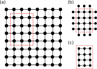
Figure 1: (a) The graph $G$. $V_{1}$ is the set of vertices in the dotted red square, and $V_{2}$ is the set of other vertices. (b) The subgraph $G^{\prime}$. (c) The subgraph $G^{\prime\prime}$.

The stabilizer test is the following test:

• Randomly generate an $N_{1}$-bit string $k\equiv(k_{1},...,k_{N_{1}})\in\{0,1\}^{N_{1}}$.

• Measure the operator

  $$s_{k}\equiv\prod_{j\in V_{1}}(g_{j}^{\prime})^{k_{j}},$$

  where $g_{j}^{\prime}$ is the stabilizer operator, Eq. (1), of the graph state $|G^{\prime}\rangle$.

• If the result is $+1$ $(-1)$, the test passes (fails).

Let $|\Psi\rangle$ be a pure state on $V$. If the probability $p_{test}$ that $|\Psi\rangle$ passes the stabilizer test satisfies $p_{test}\geq 1-\epsilon$, where $0\leq\epsilon\leq\frac{1}{2}$, then

$$\frac{1}{2}\Big{\|}|\Psi\rangle\langle\Psi|-|\Psi^{\prime}\rangle\langle\Psi^{\prime}|\Big{\|}_{1}\leq\sqrt{4\epsilon-4\epsilon^{2}},$$

where

$$|\Psi^{\prime}\rangle\equiv W(|G^{\prime\prime}\rangle\otimes|\xi\rangle_{V_{2}}).$$

Here, $|\xi\rangle$ is a certain state on $V_{2}$ and

$$W\equiv\prod_{(i,j)\in E_{connect}}CZ_{i,j}.$$

For a proof, see Ref. QSZKsingle .

V Necessity of more relaxed test

According to the theory of fault-tolerant measurement-based quantum computing, if ${\mathcal{E}}$ is not too strong, fault-tolerant measurement-based quantum computing is possible on the state ${\mathcal{E}}_{n}(|G\rangle\langle G|)$ for a certain $n$-qubit graph $G$ RHG . In particular, there exists a set $\Gamma\subset\{0,1\}^{n}$ of $n$-bit strings $\gamma$ such that fault-tolerant measurement-based quantum computing is possible on $|G_{\gamma}\rangle$. (For more details, see Sec. VIII.)

If there is some noise in the quantum channel between Merlin and Arthur, the stabilizer test introduced in the previous section is so strict that even honest Merlin is rejected with high probability. For example, let us assume that honest Merlin sends Arthur the correct state

$$W(|G^{\prime\prime}\rangle\otimes|\xi\rangle_{V_{2}}),$$

but due to the noise, what Arthur receives is

$$|\Psi\rangle=W(|G_{\gamma}^{\prime\prime}\rangle\otimes|\xi\rangle_{V_{2}})$$

where $\gamma\in\Gamma$ but $\gamma\neq 0^{N_{1}}$. Here, $\Gamma\subset\{0,1\}^{N_{1}}$ is the set of $N_{1}$-bit strings $\gamma$ such that fault-tolerant measurement-based quantum computing is possible on $|G_{\gamma}^{\prime\prime}\rangle$. (See Sec. VIII.) Then, the probability $p_{test}$ that $|\Psi\rangle$ passes the stabilizer test is

$$p_{test} = \frac{1}{2^{N_{1}}}\sum_{k\in\{0,1\}^{N_{1}}}\langle\Psi|\frac{I+s_{k}}{2}|\Psi\rangle$$

$$= \frac{1}{2}+\frac{1}{2}\langle\Psi|\prod_{j\in V_{1}}\frac{I+g_{j}^{\prime}}{2}|\Psi\rangle$$

$$= \frac{1}{2}.$$

Note that this value $1/2$ is the minimum value of $p_{test}$, since

$$\langle\Phi|\prod_{j\in V_{1}}\frac{I+g_{j}^{\prime}}{2}|\Phi\rangle\geq 0$$

for any state $|\Phi\rangle$.

Let us try to prove Theorem 2 by using the stabilizer test of the previous section. We first assume that a language $L$ is in ${\rm QMA}(a,b)$. Due to the error reducibility of QMA, the assumption $L\in{\rm QMA}(a,b)$ means that $L$ is in ${\rm QMA}(1-2^{-t},2^{-t})$ for any polynomial $t$. We want to show that $L$ is in ${\rm QMA}_{{\mathcal{E}},{\rm single}}(1-2^{-r},2^{-r})$ for any $r=poly(|x|)$. To show it, we consider a similar protocol of Ref. MNS where Arthur chooses the computation with probability $q$ and the stabilizer test with probability $1-q$. Let $p_{comp}$ be the probability of accepting the computation result when he chooses the computation, and $p_{test}$ be that of passing the stabilizer test when he chooses the stabilizer test.

First let us consider the case of $x\in L$. In this case, Merlin sends the correct state, i.e., the encoded witness state entangled with the graph state. According to the theory of fault-tolerant measurement-based quantum computing, Arthur can do the correct quantum computing on the noisy graph state with probability $1-2^{-s}$ and fails the correct computing with probability $2^{-s}$ for any polynomial $s$. The acceptance probability $p_{acc}$ is therefore

$$p_{acc} = qp_{comp}+(1-q)p_{test}$$

$$\geq q[(1-2^{-t})(1-2^{-s})+0\times 2^{-s}]+(1-q)\frac{1}{2}$$

$$= q[(1-2^{-t})(1-2^{-s})]+(1-q)\frac{1}{2}\equiv\alpha.$$

Next let us consider the case of $x\notin L$. In this case, the acceptance probability is

$$p_{acc} = qp_{comp}+(1-q)p_{test}$$

$$\leq q\times 1+(1-q)(1-\epsilon)$$

$$= q+(1-q)(1-\epsilon)\equiv\beta$$

if malicious Merlin sends a state such that $p_{test}<1-\epsilon$. The gap $\Delta$ is then

$$\Delta\equiv\alpha-\beta=q[(1-2^{-t})(1-2^{-s})-1]+(1-q)\Big{(}\epsilon-\frac{1}{2}\Big{)}\leq 0$$

for any $0\leq q\leq 1$, and therefore we cannot show $\Delta\geq 1/poly$, which is necessary to show Theorem 2.

A reason why the above proof does not work is that the probability that honest Merlin passes the stabilizer test is too small. If Merlin is honest and if the channel gives only a weak error that is correctable, what Arthur receives should be accepted with high probability, since it is useful for the correct quantum computing. This argument suggests that the stabilizer test in the previous section is too strict for several practical situations such as the noisy channel case. Hence we need a more relaxed test.

VI Proof of Theorem 2

Now we give a proof of Theorem 2 by introducing a more relaxed stabilizer test. Let us assume that a language $L$ is in ${\rm QMA}(a,b)$. Due to the error reducibility of QMA, this means that $L$ is in ${\rm QMA}(1-2^{-t},2^{-t})$ for any polynomial $t$. Therefore, without loss of generality, we take $a=1-2^{-t}$ and $b=2^{-t}$ for any polynomial $t$. Let $\{V_{x}\}_{x}$ be Arthur’s verification circuits, and $|\psi\rangle$ be the yes witness that gives the acceptance probability larger than $a=1-2^{-t}$. We consider the bipartite graph $G$ of Fig. 2. (For simplicity, the graph is written as the two-dimensional square lattice, but the graph can be more complicated depending on the computation.)

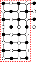
Figure 2: The graph $G$. $V_{1}$ is the set of vertices in the dotted red square, and $V_{2}$ is the set of other vertices. Two subgraphs $G^{\prime}$ and $G^{\prime\prime}$ are defined as in Sec. IV. In this example, the subgraph $G^{\prime}$ is equal to $G$.

Our protocol runs as follows.

• If Merlin is honest, he generates the correct state

  $$|\Psi_{correct}\rangle\equiv W[|G^{\prime\prime}\rangle\otimes Enc(|\psi\rangle)]$$

  on the graph $G$, where $Enc(|\psi\rangle)$ is the encoded version of $|\psi\rangle$ and placed on $V_{2}$. Merlin sends each qubit of $|\Psi_{correct}\rangle$ one by one to Arthur. If Merlin is malicious, he generates any state $|\Psi\rangle$ on $G$ and sends each qubit of it one by one to Arthur. (Due to the convexity, we can assume without loss of generality that malicious Merlin sends pure states.)

• With probability $q$, which will be specified later, Arthur does the fault-tolerant measurement-based quantum computation that implements the fault-tolerant version of $V_{x}$ with input $|\psi\rangle$. If the result is accept (reject), he accepts (rejects). We denote the acceptance probability by $p_{comp}$.

• With probability $\frac{1-q}{2}$, Arthur measures all black qubits of $G^{\prime\prime}$ in $X$ and all white qubits of $G^{\prime}$ in $Z$. Let $\{x_{j}\}_{j}$ and $\{z_{j}\}_{j}$ be the set of the $X$ measurement results and $Z$ measurement results, respectively. If and only if the syndrome set

  $$Synd_{1}\equiv\Big{\{}x_{j}\oplus\bigoplus_{i\in S_{j}}z_{i}\Big{\}}_{j\in V_{1}^{b}}$$

  satisfies certain condition $Cond_{1}$, which will be explained later, Arthur accepts. Here, $S_{j}$ is the set of the nearest-neighbour vertices of $j$th vertex in terms of the graph $G^{\prime}$, and $V_{1}^{b}$ is the set of black vertices in $V_{1}$. We denote the acceptance probability by $p_{test1}$.

• With probability $\frac{1-q}{2}$, Arthur measures all white qubits of $G^{\prime\prime}$ in $X$ and all black qubits of $G^{\prime}$ in $Z$. Let $\{x_{j}\}_{j}$ and $\{z_{j}\}_{j}$ be the set of the $X$ measurement results and $Z$ measurement results, respectively. If and only if the syndrome set

  $$Synd_{2}\equiv\Big{\{}x_{j}\oplus\bigoplus_{i\in S_{j}}z_{i}\Big{\}}_{j\in V_{1}^{w}}$$

  satisfies certain condition $Cond_{2}$, which will be explained later, Arthur accepts. Here, $V_{1}^{w}$ is the set of the white vertices in $V_{1}$. We denote the acceptance probability by $p_{test2}$.

The conditions $Cond_{1}$ and $Cond_{2}$ are taken in such a way that if $Synd_{1}$ satisfies $Cond_{1}$ and $Synd_{2}$ satisfies $Cond_{2}$ then errors are correctable, and therefore fault-tolerant measurement-based quantum computing is possible. In this paper, we do not give the explicit expressions of $Cond_{1}$ and $Cond_{2}$, since they are complicated and not necessary. At least, according to the theory of fault-tolerant quantum computing, we can define such $Cond_{1}$ and $Cond_{2}$, and the membership of $Cond_{1}$ and $Cond_{2}$ can be decided in a polynomial time. A more detailed discussion is given in Sec. VIII.

First we consider the case when $x\in L$. Since ${\mathcal{E}}$ is not too strong, $p_{test1}\geq 1-\delta$ and $p_{test2}\geq 1-\delta$ for certain $\delta=2^{-poly}$(see Sec. VIII). Therefore, the acceptance probability $p_{acc}$ is

$$p_{acc} = qp_{comp}+\frac{1-q}{2}p_{test1}+\frac{1-q}{2}p_{test2}$$

$$\geq q[(1-2^{-s})a+2^{-s}\times 0]+\frac{1-q}{2}(1-\delta)+\frac{1-q}{2}(1-\delta)$$

$$= q(1-2^{-s})a+(1-q)(1-\delta)\equiv\alpha.$$

Next we consider the case when $x\notin L$. There are four possibilities for $|\Psi\rangle$:

• $p_{test1}\geq 1-\epsilon$ and $p_{test2}<1-\epsilon$,

• $p_{test1}<1-\epsilon$ and $p_{test2}\geq 1-\epsilon$,

• $p_{test1}<1-\epsilon$ and $p_{test2}<1-\epsilon$,

• $p_{test1}\geq 1-\epsilon$ and $p_{test2}\geq 1-\epsilon$,

where $\epsilon$ is a certain parameter that will be specified later. Let us consider each case separately. First, if $p_{test1}\geq 1-\epsilon$ and $p_{test2}<1-\epsilon$,

$$p_{acc} = qp_{comp}+\frac{1-q}{2}p_{test1}+\frac{1-q}{2}p_{test2}$$

$$< q+\frac{1-q}{2}+\frac{1-q}{2}(1-\epsilon)\equiv\beta_{1}.$$

Second, if $p_{test1}<1-\epsilon$ and $p_{test2}\geq 1-\epsilon$,

$$p_{acc} = qp_{comp}+\frac{1-q}{2}p_{test1}+\frac{1-q}{2}p_{test2}$$

$$< q+\frac{1-q}{2}(1-\epsilon)+\frac{1-q}{2}=\beta_{1}.$$

Third, if $p_{test1}<1-\epsilon$ and $p_{test2}<1-\epsilon$,

$$p_{acc} = qp_{comp}+\frac{1-q}{2}p_{test1}+\frac{1-q}{2}p_{test2}$$

$$< q+\frac{1-q}{2}(1-\epsilon)+\frac{1-q}{2}(1-\epsilon)$$

$$= q+(1-q)(1-\epsilon)\equiv\beta_{2}.$$

Finally, if $p_{test1}\geq 1-\epsilon$ and $p_{test2}\geq 1-\epsilon$,

$$p_{acc} = qp_{comp}+\frac{1-q}{2}p_{test1}+\frac{1-q}{2}p_{test2}$$

$$\leq q[(1-2^{-s})b+2^{-s}\times 1+\sqrt{4\epsilon-4\epsilon^{2}}]+\frac{1-q}{2}+\frac{1-q}{2}$$

$$= q[(1-2^{-s})b+2^{-s}+\sqrt{4\epsilon-4\epsilon^{2}}]+1-q\equiv\beta_{3}.$$

Here, we have used the fact that if $p_{test1}\geq 1-\epsilon$ and $p_{test2}\geq 1-\epsilon$ then

$$\frac{1}{2}\Big{\|}|\Psi\rangle-|\Psi^{\prime}\rangle\Big{\|}_{1}\leq\sqrt{4\epsilon-4\epsilon^{2}},$$ (2)

where

$$|\Psi^{\prime}\rangle\equiv\sum_{\gamma\in\Gamma}\sum_{t}D_{\gamma,t}W(|G_{\gamma}^{\prime\prime}\rangle\otimes|\phi_{t}\rangle),$$

$\Gamma$ is the set of $\gamma$ such that errors on $|G_{\gamma}^{\prime\prime}\rangle$ are correctable, $\{D_{\gamma,t}\}_{\gamma,t}$ is the set of certain complex coefficients such that

$$\sum_{\gamma\in\Gamma}\sum_{t}|D_{\gamma,t}|^{2}=1,$$

and $\{\phi_{t}\}_{t}$ is an orthonormal basis on $V_{2}$. A proof of Eq. (2) is given in the next section.

Let us define

$$\Delta_{1}(q) \equiv \alpha-\beta_{1}=q[(1-2^{-s})a-1]+(1-q)\Big{(}\frac{\epsilon}{2}-\delta\Big{)},$$

$$\Delta_{2}(q) \equiv \alpha-\beta_{2}=q[(1-2^{-s})a-1]+(1-q)(\epsilon-\delta),$$

$$\Delta_{3}(q) \equiv \alpha-\beta_{3}=q[(1-2^{-s})(a-b)-2^{-s}-\sqrt{4\epsilon-4\epsilon^{2}}]-(1-q)\delta.$$

Then, the value $q^{*}$ that gives $\max_{q}\min(\Delta_{1},\Delta_{2},\Delta_{3})$ is $q$ such that $\Delta_{1}(q)=\Delta_{3}(q)$. Therefore,

$$q^{*}\equiv\frac{\frac{\epsilon}{2}}{1+\frac{\epsilon}{2}-(1-2^{-s})b-2^{-s}-\sqrt{4\epsilon-4\epsilon^{2}}}$$

and for this $q^{*}$, the gap is

$$\Delta_{3}(q^{*}) = \frac{\frac{\epsilon}{2}[(1-2^{-s})(a-b)-2^{-s}-\sqrt{4\epsilon-4\epsilon^{2}}]}{1+\frac{\epsilon}{2}-(1-2^{-s})b-2^{-s}-\sqrt{4\epsilon-4\epsilon^{2}}}-\delta(1-q^{*})$$

$$\geq \frac{\frac{\epsilon}{2}[(1-2^{-s})(a-b)-2^{-s}-\sqrt{4\epsilon}]}{1+\frac{\epsilon}{2}}-\delta\times 1$$

$$= \frac{\frac{\epsilon}{2}[(1-2^{-s})(1-2^{-t+1})-2^{-s}-\sqrt{4\epsilon}]}{1+\frac{\epsilon}{2}}-\delta$$

$$\geq \frac{\frac{1}{64\times 2}(\frac{7}{8}\times\frac{7}{8}-\frac{1}{8}-\frac{2}{8})}{1+\frac{1}{64\times 2}}-\delta$$

$$= \frac{25}{64^{2}\times 2+64}-\delta,$$

where we have taken $\epsilon=\frac{1}{64}$, $s\geq 3$, and $t\geq 4$. Hence $L$ is in ${\rm QMA}_{{\mathcal{E}},{\rm single}}(a^{\prime},b^{\prime})$ with $a^{\prime}-b^{\prime}\geq const.\geq 1/poly(|x|)$.

It is easy to show that if we run the above protocol in parallel, and Arthur takes the majority voting, then the error $(a^{\prime},b^{\prime})$ can be amplified to $(1-2^{-r},2^{-r})$ for any $r=poly(|x|)$. The proof is almost the same as that of the standard error reduction in QMA. One different point is, however, that when the channel is noisy, even the yes witness is not the tensor product of the original witness states, because the noise can generate entanglement among them. This means that unlike the standard QMA case, the output of each run is not independent even in the yes case, and therefore the Chernoff bound does not seem to be directly used. However, we can show that the probability of obtaining 0 in the $i$th run is upperbounded by $1-a$ whatever results obtained in the previous runs. Therefore, the rejection probability is upperbounded by that of the case when each run is the independent Bernoulli trial with the coin bias $(1-a,a)$, where the standard Chernoff bound argument works. (More precisely, the argument is as follows. In the first run, the probability of obtaining 0 is $Pr[y_{1}=0]\leq 1-a$, where $y_{1}$ is the result of the first run. If we assume $Pr[y_{1}=0]=1-a$, we can maximize the rejection probability. In the second run, the probability of obtaining 0 is $Pr[y_{2}=0|y_{1}]\leq 1-a$. If we assume $Pr[y_{2}=0|y_{1}]=1-a$, we can maximize the rejection probability. If we repeat it for all runs, we conclude that the the independent Bernoulli trial with the coin bias $(1-a,a)$ achieves the maximum rejection probability. According to the Chernoff bound, the maximum rejection probability is upperbounded by an exponentially decaying function. ) $\blacksquare$

VII Proof of Eq. (2)

In this section, we show Eq. (2). Let us define $N_{1}^{b}\equiv|V_{1}^{b}|$ and $N_{1}^{w}\equiv|V_{1}^{w}|$. Since $p_{test1}\geq 1-\epsilon$,

$$p_{test1}=\sum_{\omega\in\Omega_{1}}\langle\Psi|\prod_{j\in V_{1}^{b}}\frac{I+(-1)^{\omega_{j}}g_{j}^{\prime}}{2}|\Psi\rangle\geq 1-\epsilon,$$ (3)

where $\Omega_{1}$ is the set of $N_{1}^{b}$-bit string $\omega=\{\omega_{j}\}_{j\in V_{1}^{b}}\in\{0,1\}^{N_{1}^{b}}$ such that $\omega$ satisfies $Cond_{1}$, and $g_{j}^{\prime}$ is the stabilizer operator of $|G^{\prime}\rangle$ on $j$th qubit. Since

$$\Big{\{}W(|G_{(u,v)}^{\prime\prime}\rangle\otimes|\phi_{t}\rangle)\Big{\}}_{u\in\{0,1\}^{N_{1}^{b}},v\in\{0,1\}^{N_{1}^{w}},t\in\{0,1\}^{N_{2}}}$$

is an orthonormal basis, we can write

$$|\Psi\rangle=\sum_{u\in\{0,1\}^{N_{1}^{b}}}\sum_{v\in\{0,1\}^{N_{1}^{w}}}\sum_{t\in\{0,1\}^{N_{2}}}C_{u,v,t}W(|G_{(u,v)}^{\prime\prime}\rangle\otimes|\phi_{t}\rangle),$$

with certain complex coefficients $\{C_{u,v,t}\}_{u,v,t}$ such that $\sum_{u,v,t}|C_{u,v,t}|^{2}=1$. Let $\{g_{j}^{\prime\prime}\}_{j}$ be the set of stabilizer operators of the graph state $|G^{\prime\prime}\rangle$. Then, it is easy to check

$$g_{j}^{\prime}W=Wg_{j}^{\prime\prime}$$

for all $j\in V_{1}$. Therefore, from Eq. (3),

$$1-\epsilon \leq \sum_{\omega\in\Omega_{1}}\langle\Psi|\prod_{j\in V_{1}^{b}}\frac{I+(-1)^{\omega_{j}}g_{j}^{\prime}}{2}|\Psi\rangle$$

$$= \sum_{\omega\in\Omega_{1}}\langle\Psi|\prod_{j\in V_{1}^{b}}\frac{I+(-1)^{\omega_{j}}g_{j}^{\prime}}{2}\sum_{u,v,t}C_{u,v,t}W(|G_{(u,v)}^{\prime\prime}\rangle\otimes|\phi_{t}\rangle)$$

$$= \sum_{\omega\in\Omega_{1}}\langle\Psi|W\prod_{j\in V_{1}^{b}}\frac{I+(-1)^{\omega_{j}}g_{j}^{\prime\prime}}{2}\sum_{u,v,t}C_{u,v,t}(|G_{(u,v)}^{\prime\prime}\rangle\otimes|\phi_{t}\rangle)$$

$$= \sum_{\omega\in\Omega_{1}}\langle\Psi|W\sum_{v}\sum_{t}C_{\omega,v,t}(|G_{(\omega,v)}^{\prime\prime}\rangle\otimes|\phi_{t}\rangle)$$

$$= \sum_{\omega\in\Omega_{1}}\sum_{v}\sum_{t}|C_{\omega,v,t}|^{2}.$$

In a similar way, $p_{test2}\geq 1-\epsilon$ leads to

$$\sum_{u}\sum_{\omega^{\prime}\in\Omega_{2}}\sum_{t}|C_{u,\omega^{\prime},t}|^{2}\geq 1-\epsilon,$$

where $\Omega_{2}$ is the set of $\omega$ that satisfy $Cond_{2}$.

Let us define

$$|\Psi^{\prime}\rangle\equiv\frac{1}{\sqrt{R}}\sum_{u\in\Omega_{1}}\sum_{v\in\Omega_{2}}\sum_{t}C_{u,v,t}W(|G_{(u,v)}^{\prime\prime}\rangle\otimes|\phi_{t}\rangle)$$

where

$$R\equiv\sum_{u\in\Omega_{1}}\sum_{v\in\Omega_{2}}\sum_{t}|C_{u,v,t}|^{2}\leq 1$$

is the normalization constant. Then,

$$\langle\Psi|\Psi^{\prime}\rangle = \frac{1}{\sqrt{R}}\sum_{u\in\Omega_{1}}\sum_{v\in\Omega_{2}}\sum_{t}|C_{u,v,t}|^{2}$$

$$\geq \sum_{u\in\Omega_{1}}\sum_{v\in\Omega_{2}}\sum_{t}|C_{u,v,t}|^{2}$$

$$\geq 1-2\epsilon.$$

Here, in the last inequality, we have used the relation

$$YY \geq YY-NN$$

$$= YY-(1-YY-YN-NY)$$

$$= (YY+YN)+(YY+NY)-1$$

$$\geq (1-\epsilon)+(1-\epsilon)-1$$

$$= 1-2\epsilon,$$

where

$$YY = \sum_{u\in\Omega_{1}}\sum_{v\in\Omega_{2}}\sum_{t}|C_{u,v,t}|^{2},$$

$$YN = \sum_{u\in\Omega_{1}}\sum_{v\notin\Omega_{2}}\sum_{t}|C_{u,v,t}|^{2},$$

$$NY = \sum_{u\notin\Omega_{1}}\sum_{v\in\Omega_{2}}\sum_{t}|C_{u,v,t}|^{2},$$

$$NN = \sum_{u\notin\Omega_{1}}\sum_{v\notin\Omega_{2}}\sum_{t}|C_{u,v,t}|^{2}.$$

Therefore, for $0\leq\epsilon\leq\frac{1}{2}$,

$$\frac{1}{2}\Big{\|}|\Psi\rangle\langle\Psi|-|\Psi^{\prime}\rangle\langle\Psi^{\prime}|\Big{\|}_{1} = \sqrt{1-|\langle\Psi|\Psi^{\prime}\rangle|^{2}}$$

$$\leq \sqrt{1-(1-2\epsilon)^{2}}$$

$$= \sqrt{4\epsilon-4\epsilon^{2}}.$$

VIII Correctability of errors

Let us consider an $n$-qubit graph state $|G\rangle$ and a tensor product $P$ of $n$ Pauli operators. When $P$ acts on $|G\rangle$, an $X$ operator in $P$ can always be changed into the tensor product of nearest-neighbour $Z$ operators by using the stabilizer relation. Therefore, we can always find $u\in\{0,1\}^{n}$ such that

$$P|G\rangle=\Big{(}\bigotimes_{j=1}^{n}Z_{j}^{u_{j}}\Big{)}|G\rangle=|G_{u}\rangle~{}(\mbox{up to phase}).$$

Hence let us consider only $Z$ errors and error is specified by $u\in\{0,1\}^{n}$. Let $\{\mathcal{M}_{a}\}_{a}$ be a POVM corresponding to a fault-tolerant measurement-based quantum computation, where $a$ is the output of the computation. Then if

$${\rm Tr}[\mathcal{M}_{a}(|G\rangle\langle G|)]={\rm Tr}[\mathcal{M}_{a}(|G_{u}\rangle\langle G_{u}|)]$$

for all $a$, $u$ is called a correctable error. The conditions, $Cond_{1}$ and $Cond_{2}$, are given as the sets of syndromes on $|G_{u}\rangle$ for all correctable errors $u$. An explicit form of the POVM depends on the fault-tolerant scheme chosen, and therefore so does the set of correctable errors. Most fault-tolerant schemes in the measurement-based model are constructed by (or at least can be regarded as) simulation of circuit-based fault-tolerant schemes. For example, fault-tolerant schemes in Ref. RHG and Refs. DHN1 ; DHN2 can be viewed as circuit-based fault-tolerant schemes using the Steane 7-qubit code and the surface code, respectively. In the fault-tolerant theory for the circuit model, a set of sparse errors are defined such that they do not change the output of the quantum computation under fault-tolerant quantum error correction BA . Therefore it is straightforward to find a correctable set $\Gamma$ of errors by directly translating the set of sparse errors in the existing circuit-based fault-tolerant schemes into errors on the graph state in the measurement-based model. A channel ${\mathcal{E}}_{n}$ is not too strong so that errors are correctable with high probability if

$$\mbox{Tr}\Big{(}\sum_{u\in\Gamma}|G_{u}\rangle\langle G_{u}|{\mathcal{E}}_{n}(|G\rangle\langle G|)\Big{)}\geq 1-\delta.$$

Here, $\delta=2^{-poly(n)}$ for natural noises. (In this paper, the proof holds even for sufficiently small constant $\delta$.) According to the theory of fault-tolerant quantum computation, under a natural physical assumption like spatial locality of noise, if noise strength of each noisy operation is sufficiently smaller than a certain threshold value, the above condition is satisfied RHG ; DHN1 ; DHN2 ; BA ; AL .

References

(1)
R. Raussendorf and H. J. Briegel,
A one-way quantum computer.
Phys. Rev. Lett. 86, 5188 (2001).
(2)
M. McKague,
Interactive proofs for BQP via self-tested graph states.
Theory of Computing 12, 1 (2016).
(3)
T. Morimae, D. Nagaj, and N. Schuch,
Quantum proofs can be verified using only single qubit measurements.
Phys. Rev. A 93, 022326 (2016).
(4)
T. Morimae,
Quantum Arthur-Merlin with single-qubit measurements.
Phys. Rev. A 93, 062333 (2016).
(5)
T. Morimae,
Quantum state and circuit distinguishability with single-qubit
measurements.
arXiv:1607.00574
(6)
M. Hayashi and T. Morimae,
Verifiable measurement-only blind quantum computing with stabilizer
testing.
Phys. Rev. Lett. 115, 220502 (2015).
(7)
K. Fujii and M. Hayashi,
in preparation.
(8)
J. F. Fitzsimons and T. Vidick,
A multiprover interactive proof system for the local Hamiltonian
problem.
Proc. of the 6th ITCS, pp.103-112 (2015).
(9)
Z. Ji, Classical verification of quantum proofs.
Proc. of the 48th STOC, pp.885-898 (2016).
(10)
M. A. Nielsen and I. L. Chuang,
Quantum Computation and Quantum Information (Cambridge University
Press, Cambridge 2000).
(11)
R. Raussendorf, J. Harrington, and K. Goyal,
Topological fault-tolerance in cluster state quantum computation.
New J. Phys. 9, 199 (2007).
(12)
C. M. Dawson, H. L. Haselgrove, and M. A. Nielsen,
Noise thresholds for optical cluster-state quantum computation.
Phys. Rev. A 73, 052306 (2006).
(13)
C. M. Dawson, H. L. Haselgrove, and M. A. Nielsen,
Noise thresholds for optical quantum computers.
Phys. Rev. Lett. 96, 020501 (2006).
(14)
D. Aharonov, and M. Ben-Or,
Fault-tolerant quantum computation with constant error.
Proc. of the 20th STOC, pp. 176-188 (1997).
(15)
P. Aliferis and D. W. Leung,
Simple proof of fault tolerance in the graph-state model.
Phys. Rev. A 73, 032308 (2006).