Scrutinizing a di-photon resonance at the LHC through Moscow zero

Abstract

The ATLAS and CMS collaborations have recently released their new analyses of the diphoton searches. We look in detail the consequences of their results deriving strong constraints on models where a scalar resonance $s$ decays into two light pseudoscalars which in turn decay into two pairs of collimated photons, mis-identified with two real photons. In our construction, all mass terms are generated dynamically, and only one pair of vector-like fermions generate couplings which will be probed using the upcoming LHC data. Moreover, we show that a stable dark matter candidate, respecting the cosmological constraints, is naturally affordable in the model.

1 Introduction

The detection of events with multi-photon final state at the LHC would represent one of the most distinct and accurate evidences of physics Beyond the Standard Model (BSM). The study of these kinds of events has encountered, in recent times, an increased interest from the Particle Physics community as a consequence of the announcement of a 3.9$\sigma$ (3.4$\sigma$) local excess in the diphoton channel by the ATLAS [1, 2] (CMS [3, 4]) group, corresponding to a 750 GeV resonance with a cross-section $\sigma_{\gamma\gamma}\sim 4-16$ fb [2]. One straightforward interpretation of this excess consists of the introduction of a spin-0 resonance coupled, at least to the gluons and the photons (as well as the $Z$ boson from gauge invariance) through dimension-5 operators of the form $\frac{c_{VV}}{\Lambda}V_{\mu\nu}V^{\mu\nu}\Phi$[5, 6, 7, 8, 9] with $\Lambda$ being the effective scale of these new interactions. The most widely studied origin of these dimension-5 operators is represented by new fermionic degrees of freedom, charged under color and hypercharge and vector-like with respect to the Standard Model (SM)  [10]. These new degrees of freedom induce, through triangle loops, couplings between the 750 GeV resonance and gluon/photons which can be described through the aforementioned dimension-5 operators upon integrating out the new fermions.

Although the most recent measurements [11, 12] seem not to confirm the existence of such a resonance (at least for a (pseudo-)scalar particle), scenario where spin-0 states are coupled with new fermions, having non-trivial quantum numbers under the SM gauge group, and detectable in diphoton events remains a natural and intriguing option to study. Indeed, as proven for example in refs. [13, 14, 15, 16, 17, 18, 19, 20, 21], in order to achieve a production cross-section of the order of the current experimental sensitivity, possibly accompanied by a sizable decay width, one should require either (1) large and possibly non-perturbative, i.e., $>\sqrt{4\pi}$, Yukawa couplings between the new BSM fermions and the 750 GeV resonance or (2) large number of new fermions or (3) large hypercharge assignment for these BSM fermions, unless rather particular setups are realized [22, 23, 24]. However, when one or more of these conditions are met then the behavior of the theory at scales above but not too far from the mass of the new fermions might become problematic. For example, condition (1) would cause a departure of the new Yukawa couplings, at low scales, from the perturbative regime while the last conditions would be associated to the occurrence of a Landau pole (a.k.a. Moscow zero) [25] for the SM gauge couplings. Furthermore, the quartic coupling present in the new scalar sector, producing the diphoton resonance, would rapidly be driven to negative value, making the theory pathological.

It would then be intriguing to compare the current experimental limits with the requirement of having a consistent perturbative theory at least up to some energy scale $\Lambda_{\rm NP}$, where a further Ultra-Violet (UV) completion should be invoked. This problem can also be reformulated by choosing a priori the scale $\Lambda_{\rm NP}$ and determining the accessible values of an hypothetical future new detection, as function of the mass of the resonance and the diphoton production cross-section.

To perform a study of this kind we consider the case in which the SM is extended by a SM gauge singlet complex scalar field $\Phi$ charged under a new global $U(1)$ symmetry, which can be interpreted as a Peccei - Quinn symmetry for instance [26]. This global symmetry is spontaneously broken by the vacuum expectation value (vev) of the scalar component of $\Phi$. The pseudoscalar component of $\Phi$ is promoted to be a light pseudo Goldstone boson by introducing small explicit violation of this new global symmetry. In this setup a diphoton signal would be originated from pairs of highly collimated photons, produced by the decay of a pair of light pseudoscalars which in turn are originated by the decay of the scalar component of $\Phi$, resonantly produced in proton-proton collision (see figure 1). The advantage of this construction is that the four-photon, i.e., the effective diphoton, cross-section can more easily attain larger values since it is controlled by branching fraction (Br) of the decay of the scalar component of $\Phi$ into two pseudoscalars, which can easily be pushed to one. This would imply, in construction involving vector-like fermions for the generation of couplings with gluons and photons, a lower multiplicity for the additional fermions. Another interesting feature is that the complementary signals like dijets, $ZZ$ and $Z\gamma$ are generally suppressed, rendering the model easy to discriminate. A similar framework giving collimated photons is the Next-to Minimal Supersymmetric Standard Model (NMSSM) [28, 29, 30] in which the new scalar and pseudoscalar fields are part of an extended Higgs sector. In this scenario a sizable production cross-section is achieved through triangle loop of the SM fermions, at the price of a very definite range of the pseudoscalar mass to avoid an otherwise highly suppressed branching fraction into photons.

The setup discussed above has previously been sketched in ref. [33] along with the introduction of a Dark Matter (DM) candidate. Interestingly, the mass term for the DM is dynamically generated by the vev of the field $\Phi$. This setup appears successful in fitting for instance the (now–dead) 750 GeV excess compatibly with the viable DM relic density without conflicting with bounds from DM detection, contrary to what would happened in the case of a “true” diphoton signal [34, 35, 36]. In this work we will present a more complete anomaly–free and UV version of the model presented in ref. [33] so that, similar to the DM interactions, the couplings among the field $\Phi$ and the SM gauge bosons are also dynamically generated. Indeed, the particle spectrum of the theory will be extended with new BSM fermionic states, vector-like with respect to the SM but chiral with respect to the new $U(1)$ symmetry, whose mass terms are generated by spontaneous breaking of the associated $U(1)$ symmetry. This kind of scenario is very predictive since it features, as free parameters, only masses of the new states (resonant scalar, new vector-like fermions and the DM) and one fundamental coupling, i.e. the quartic coupling $\lambda$ of the $\Phi$ field.

We will show that asking for the stability of the $\Phi$ potential ($\lambda$ positive up to a energy scale $\Lambda_{\rm NP}$, beyond with “further” New Physics appears essential) provides constraints competitive with the experimental ones. In particular, the masses of the new fermions are restricted to lie below 2 TeV, well within the kinematical reach of LHC run-II. By further combining the requirements of theoretical consistency and a near future detection of the diphoton signal with correct relic density, an even more constrained scenario, giving definite predictions of the DM mass, is achieved.

The paper is structured as follows. We first discuss an overview of the model in section 2 and then provide the relevant expressions for the 4-photon production cross-section. In the following section we investigate the UV behavior of the theory by studying the relevant Renormalization Group Equations (RGEs). In section 4 we address the DM phenomenology. We summarize our results and discuss the associated implications in section 5 before we put our concluding remarks in section 6. Some useful formulas are relegated to the appendix.

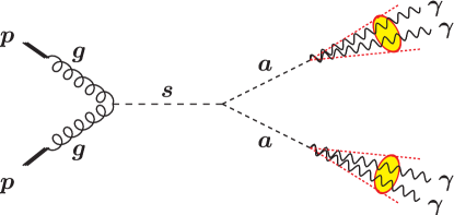
Figure 1: Feynman diagram producing a 4-photon final state that is mis-identified as a diphoton signal.

2 The Model

2.1 The Lagrangian

We minimally extend the Standard Model by introducing a complex scalar field $\Phi=(s+ia)/\sqrt{2}$, singlet under the SM gauge group, whose Lagrangian can be written as:

$${\cal L}_{\Phi}=\partial_{\mu}\Phi\partial^{\mu}\Phi^{*}+\mu_{\Phi}^{2}|\Phi|^{2}-\lambda|\Phi|^{4}+\frac{\epsilon_{\Phi}^{2}}{2}(\Phi^{2}+\text{~{}h.c.}).$$ (2.1)

We can see from eq. (2.1) that the last term ($\epsilon_{\Phi}\ll\mu_{\Phi}$) explicitly breaks the $U(1)$ symmetry, giving mass to the otherwise massless Goldstone boson $a$, which is then promoted to a light pseudo-Goldstone state. We also introduce new Dirac fermions $F_{L},F_{R}$, chiral under the new $U(1)$ symmetry with different charge assignments but vector-like under the SM gauge group, having non trivial $SU(3)_{C}$ and $U(1)_{Y}$ quantum numbers but singlet with respect to $SU(2)_{L}$. With these assumptions the relevant Lagrangian for the new fermions is:

$${\cal L}_{F}=i\bar{F}_{L}\gamma^{\mu}D_{\mu}F_{L}+i\bar{F}_{R}\gamma^{\mu}D_{\mu}F_{R}-(y_{F}\Phi\bar{F}_{L}F_{R}+\text{h.c.})=i\bar{F}\gamma^{\mu}D_{\mu}F-\frac{y_{F}}{\sqrt{2}}s\bar{F}F-i\frac{y_{F}}{\sqrt{2}}a\bar{F}\gamma^{5}F,$$ (2.2)

where $D_{\mu}$ is the SM covariant derivative and $F\equiv F_{L}+F_{R}$.

Once $\Phi$ acquires a vev through the spontaneous symmetry breaking mechanism, $\Phi=(v_{\Phi}+s+ia)/\sqrt{2}$ with $v^{2}_{\Phi}=(\mu_{\Phi}^{2}+\epsilon^{2}_{\Phi})/\lambda\simeq\mu_{\Phi}^{2}/\lambda$, it generates automatically the mass of $s$ ($m_{s}=\sqrt{2\lambda}v_{\Phi}$), the $saa$ coupling ($\lambda_{saa}=\lambda v_{\Phi}$), and masses of the new fermions ($m_{F}=y_{F}v_{\Phi}/\sqrt{2}$). The pseudoscalar mass is given by $m_{a}=\sqrt{2}\epsilon_{\Phi}$. Re-expressing the Lagrangian, after spontaneous symmetry breaking, as a function of the physical fields gives :

$$-{\cal L}\supset\frac{m_{s}^{2}}{2}s^{2}+\frac{m_{a}^{2}}{2}a^{2}+\sqrt{\frac{\lambda}{2}}m_{s}sa^{2}+\sqrt{\frac{\lambda}{2}}m_{s}s^{3}+\frac{\lambda}{4}(s^{2}+a^{2})^{2}+m_{F}\bar{F}F+\sqrt{2\lambda}\frac{m_{F}}{m_{s}}(s\bar{F}F+ia\bar{F}\gamma^{5}F),$$ (2.3)

where we have used $y_{F}=\sqrt{2}m_{F}/v_{\Phi}=2\sqrt{\lambda}(m_{F}/m_{s})$. We note in passing that in the current article, for simplicity and enhanced predictability, we have assumed vanishing mixing between $\Phi$ and the SM-Higgs. This choice is also motivated by the fact that this mixing is in general strongly constrained. For example, it would lead to non-standard decays of the SM-Higgs, e.g., SM-Higgs to a pair of light pseudoscalars. Similarly, a sizable mixing between $\Phi$ and the SM-Higgs would appear strongly disfavored by the DM phenomenology. Indeed it would induce a coupling between the DM and the SM-Higgs, responsible for a potentially strong Spin Independent component of the DM scattering cross-section with nucleons, which would be in tension with the current experimental limits [39].

2.2 Generating the vertices

Effective couplings between the SM gauge fields and the complex scalar field $\Phi$ are generated through a triangular loop (see figure 2) involving the new fermions, $F$. In this work the new fermion sector will be composed by $N_{f}$ “families”; each one comprised of a pair of degenerate fermions, chiral under the new $U(1)$ symmetry and belonging to the fundamental representation of $SU(3)_{C}$, singlet under $SU(2)_{L}$ and, with electric charges $\pm Q_{F}$ (i.e., the $U(1)_{Y}$ charges), in order to represent an anomaly free configuration. We observe that the main purpose of this paper is to provide a proof of existence of the correlation between hypothetical signals of collimated photons, UV consistency of the underlying theory and DM phenomenology. As a consequence, we have presumed some simplifying assumptions. We have indeed considered, throughout this work, that both the production process (gluon fusion) and the decay of the scalar resonance into $4\gamma$ are originated by the same fermion fields, which are, thus, both electrically and color charged. As further assumption we have considered only integer values for $Q_{F}$. Our results could be straightforwardly extended to more generic assumptions concerning the parameters of the new fermionic sector. It is worthy to note here that strong experimental bounds exist on the masses of vector-like quarks [40, 41], on exotic particles having higher electric charges $(2|e|-6|e|)$ [42] or on lepton-like fermions with $Q_{F}=1|e|,\,2|e|$ [43]. However, experimental constraints on colored vector-like fermions having integral electric charges, as considered in this article, remain rather inadequate till date.

In this setup the relevant Lagrangian can be expressed as [33]:

$$-{\cal L}\supset\frac{\sqrt{\lambda}C_{GG}}{m_{s}}sG_{\mu\nu}^{\alpha}G^{\mu\nu}_{\alpha}+\frac{\sqrt{\lambda}\widetilde{C}_{GG}}{m_{s}}aG_{\mu\nu}^{\alpha}\widetilde{G}^{\mu\nu}_{\alpha}+\frac{\sqrt{\lambda}C_{BB}c_{W}^{2}}{m_{s}}sF_{\mu\nu}F^{\mu\nu}+\frac{\sqrt{\lambda}\widetilde{C}_{BB}c_{W}^{2}}{m_{s}}aF_{\mu\nu}\widetilde{F}^{\mu\nu},$$ (2.4)

where $F_{\mu\nu}$ and $G_{\mu\nu}^{\alpha}$ ($\widetilde{F}_{\mu\nu}$ and $\widetilde{G}_{\mu\nu}^{\alpha}$) are the field (dual field) strengths for the photon and gluons, respectively. Here $c^{2}_{W}\equiv\cos^{2}\theta_{W}=0.769$ [44], with $\theta_{W}$ being the Weinberg angle, and the coefficients (details are given in the appendix):

$$C_{GG}=N_{f}\frac{\alpha_{s}}{4\sqrt{2}\pi}f_{1/2}(m_{s}^{2}/4m_{F}^{2}),\,\,\,C_{BB}=N_{f}\frac{3\alpha_{em}}{2\sqrt{2}\pi c_{W}^{2}}Q^{2}_{F}f_{1/2}(m_{s}^{2}/4m_{F}^{2}),$$

$$\widetilde{C}_{GG}=N_{f}\frac{\alpha_{s}}{4\sqrt{2}\pi}\tilde{f}_{1/2}(m_{a}^{2}/4m_{F}^{2}),\,\,\,\widetilde{C}_{BB}=N_{f}\frac{3\alpha_{em}}{2\sqrt{2}\pi c_{W}^{2}}Q_{F}^{2}\tilde{f}_{1/2}(m_{a}^{2}/4m_{F}^{2}),$$ (2.5)

where $\alpha_{s},\,\alpha_{em}$ are the strong and electromagnetic coupling constants and the functions $f_{1/2}(m_{s}^{2}/4m_{F}^{2})$, $\tilde{f}_{1/2}(m_{a}^{2}/4m_{F}^{2})$ are described in the appendix. Note that the presence of $Q^{2}_{F}$ in the expressions for $C_{BB},\,\widetilde{C}_{BB}$ makes them insensitive to the sign of $Q_{F}$. It is evident from eq. (2.4) that the scale of dimension-5 operators $\Phi V^{\mu\nu}V_{\mu\nu}$ corresponds to the vev $v_{\Phi}\propto{m_{s}}/{\sqrt{\lambda}}$ of the complex scalar field. The coefficients in eq. (2.2) are substantially insensitive to $m_{s}$, $m_{a}$ and the masses of new fermions $m_{F}$. From now on -unless differently stated- we will consider, throughout this work, the case of only one pair of new fermions, i.e., $N_{f}=1$.

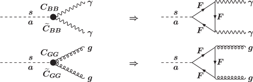
Figure 2: Loop triangle diagram generating interactions among the photons and gluons with the real $(s)$ and imaginary $(a)$ components of $\Phi$. The first diagram, from the principle of gauge invariance, will also generate effective interactions like $sZ\gamma,\,sZZ$, etc, however, their relative strengths will be different from $s\gamma\gamma$ [33].

2.3 The 4$\gamma$ production

In this scenario, the diphoton signal is mostly originated from the process $gg\rightarrow s\rightarrow aa\rightarrow 4\gamma$, whose corresponding diagram is shown in figure 1. Given a sufficiently light pseudoscalar, the boosted photon pairs originated from its decay might appear enough collimated to be mis-identified as a single photon.

As minimal requirement to achieve such degree of collimation, one needs to impose that the opening angle between the collimated photons remains below the detector resolution of the LHC, $\sim\mathcal{O}($20 mrad). This can be accomplished by imposing the boost factor $\gamma\simeq\frac{m_{s}}{2m_{a}}\gtrsim 200$ [45] implying:

$$m_{a}\lesssim 2.5~{}\mathrm{GeV}\left(\frac{m_{s}}{1~{}\mathrm{TeV}}\right),$$ (2.6)

and thus, obtaining an upper bound on the mass of the pseudoscalar for a fixed $m_{s}$. On the other hand, such a low mass might produce large lifetime for the pseudoscalar field such that it decays beyond the Electromagnetic CALorimeter (ECAL) which lies at a distance of $\mathcal{O}(1$ m) from the primary interaction point. Such situation mainly arises for $m_{a}\lesssim 3m_{\pi_{0}}$ since in this case the pseudoscalar can only decay into photon pairs. In this setup, requiring a decay length $l\lesssim 1\,\mbox{m}$ translates into the following relation:

$$l\simeq 71~{}\mathrm{m}\left(\frac{m_{s}}{1~{}\mathrm{TeV}}\right)^{3}\left(\frac{0.5~{}\mathrm{GeV}}{m_{a}}\right)^{4}\frac{1}{N^{2}_{f}Q_{F}^{4}}\left(\frac{0.01}{\lambda}\right),$$ (2.7)

which can be used to extract a lower bound on $m_{a}$. In the case of $m_{s}=750\,\mbox{GeV}$ for instance, the combination of eq. (2.6) and eq. (2.7) fixes the value of $m_{a}$ to lie within the range $0.2$ GeV $\lesssim m_{a}\lesssim$ 2 GeV [33, 46, 26]. This mass range could be restricted further by a more dedicated investigation of the ECAL response [46, 26] and/or by including the effects of photon conversions [47]. These kinds of analyses are, however, beyond the scopes of this paper.

The 4$\gamma$ production cross-section, following figure 1, can be straightforwardly computed as:

$$\sigma_{4\gamma}=\frac{\pi^{2}}{8m_{s}\bf{s}}\Gamma(s\rightarrow gg)\mathrm{Br}(s\rightarrow aa)[\mathrm{Br}(a\rightarrow\gamma\gamma)]^{2}I_{GG}(m_{s}/\sqrt{\bf{s}}),$$ (2.8)

where $\sqrt{{\bf s}}=13\,\mbox{TeV}$ is the present LHC center-of-mass energy, $\Gamma(s\rightarrow gg)$ is the decay width of $s\to gg$ process and $I_{GG}(m_{s}/\sqrt{\bf{s}})$ is the integral representing the effect of the parton distribution functions (PDFs). For the computation of $I_{GG}(m_{s}/\sqrt{\bf{s}})$ we have used the MSTW2008NNLO distribution [48, 49, 50].

It can be easily verified that, in the parameter space relevant for $gg\to s\to aa\to 4\gamma$ process, $\mathrm{Br}(s\rightarrow aa)\sim 1$ [33]. As already pointed out, for $m_{a}<3m_{\pi^{0}}$, only decay into the photon pairs is accessible, so the 4$\gamma$ production cross-section depends only on the coupling $C_{GG}$ (contained in $\Gamma(s\rightarrow gg)$) between the resonance and the gluons. Thus, eq. (2.8), using eq.(2.2), can be simplified as:

$$\sigma_{4\gamma}\simeq 1.64~{}\mathrm{fb}\frac{(\Gamma_{s}/m_{s})}{10^{-4}}\left(\frac{I_{GG}(m_{s}/\sqrt{\bf{s}})}{2000}\right)N^{2}_{f}\,\simeq 0.33~{}\mathrm{pb}\left(\frac{I_{GG}(m_{s}/\sqrt{\bf{s}})}{2000}\right)N^{2}_{f}\lambda,$$

$$\hskip 256.0748pt\left[\rm{for~{}}m_{a}\lesssim 3m_{\pi^{0}}\right],~{}~{}$$ (2.9)

here $\Gamma_{s}$ represents the total width of scalar resonance $s$, which is $\approx\Gamma(s\to aa)$ when diphoton signal is arising from collimated photons. For numerical estimates we have used values of $\alpha_{em},\,\alpha_{s}$ at the energy scale $m_{Z}$ [44].

In the case of $m_{a}\gtrsim 3\,m_{\pi^{0}}$, the production cross-section should be rescaled by a factor $\mathrm{Br}(a\rightarrow\gamma\gamma)^{2}\approx\frac{81}{4}\frac{\alpha_{\rm em}^{4}}{\alpha_{\rm s}^{4}}Q_{F}^{8}$ and is given by:

$$\sigma_{4\gamma}\simeq 0.63~{}\mathrm{fb}\frac{(\Gamma_{s}/m_{s})}{0.1}\left(\frac{I_{GG}(m_{s}/\sqrt{\bf{s}})}{2000}\right)N^{2}_{f}Q^{8}_{F}\simeq 0.12~{}\mathrm{fb}\,\,\left(\frac{I_{GG}(m_{s}/\sqrt{\bf{s}})}{2000}\right)N^{2}_{f}Q^{8}_{F}\,\lambda,$$

$$\hskip 227.62204pt\left[\rm{for}~{}m_{a}\gtrsim 3m_{\pi^{0}}\right].\,\,$$ (2.10)

Just like the pseudoscalar field, the scalar field $s$ is also coupled to photons through the same set of new BSM fermions (see figure 2). Thus, one should in general also account for the direct diphoton production from the decay of scalar resonance. The conditions for the dominance of 4-photon production cross-section over the 2-photon $(\sigma_{2\gamma})$ have already been determined in ref. [33] in terms of the effective coupling coefficients. In the dynamical realization, considered in this work, these conditions can be translated as:

$$C_{\rm BB}<0.65\rightarrow\sqrt{N_{f}}Q_{F}\lesssim 11,\,\,\,\,\,\,\,\left[\rm{for}~{}m_{a}<3m_{\pi^{0}}\right],$$

$$\widetilde{C}_{\rm GG}<0.27\widetilde{C}_{\rm BB}/\sqrt{C_{\rm BB}}\rightarrow Q_{F}/\sqrt{N_{f}}\lesssim 1\,\,\,\,\,\,\,\left[\rm{for}~{}m_{a}>3m_{\pi^{0}}\right],$$ (2.11)

while the “true” diphoton production cross-section $\sigma_{2\gamma}$ can be written as:

$$\sigma_{2\gamma}=\frac{\pi^{2}}{8m_{s}\bf{s}}\Gamma(s\rightarrow gg)\mathrm{Br}(s\rightarrow\gamma\gamma)I_{GG}(m_{s}/\sqrt{\bf{s}})\,\,\simeq 3.7\times 10^{-4}~{}\mathrm{fb}\,\,\frac{N^{4}_{f}Q^{4}_{F}}{(\Gamma_{s}/m_{s})}\left(\frac{I_{GG}(m_{s}/\sqrt{\bf{s}})}{2000}\right)\lambda^{2}.$$ (2.12)

We notice that in the regime $m_{a}<3m_{\pi^{0}}$, the contribution to the collective diphoton, i.e., $2\gamma+4\gamma$, production from $s\to\gamma\gamma$ process is practically negligible unless one considers very high fermion multiplicities and/or high electric charges. In the opposite regime, in the case of $N_{f}=1$ and $Q_{F}\leq 2$, which will be considered throughout most of this work, a sub-dominant but non-vanishing contribution from the $gg\rightarrow s\rightarrow\gamma\gamma$ process is present. Although the analytical estimates presented in the current and the following subsection will rely only on the 4-photon production cross-section, nevertheless, in our numerical analysis we have also included the 2-photon production cross-section.

One can easily see from eq. (2.9) and eq. (2.3), that the 4-photon production cross-section is mostly determined by the parameters $\lambda$ (and $Q_{F}$ for $m_{a}>3m_{\pi^{0}}$) while the dependence on $m_{s}$ is encoded only in the integral $I_{\rm GG}(m_{s}/\sqrt{\bf{s}})$. It is then possible to translate the observed limits by the ATLAS [11] and CMS [12] collaborations on the diphoton production cross-section directly into limit on the value of $\lambda$. These would particularly give stringent bound on $\lambda$ in the $m_{a}\lesssim 3m_{\pi^{0}}$ case, for example, $\lambda\lesssim 3\times 10^{-2}$ for $m_{s}=1$ TeV, using the latest experimental result [12].

By comparing eq. (2.9) in the light of eq. (2.7), we also notice that the requirement of a decay length for the pseudoscalar $\raise 1.29167pt\hbox{$\;<$\kern-7.5pt\raise-4.73611pt\hbox{$\sim\;$}}1$ m would imply a lower limit on the 4$\gamma$ as:

$$\sigma_{4\gamma}\gtrsim 232\,\mathrm{fb}\frac{1}{Q_{F}^{4}}\frac{I_{GG}(m_{s}/\sqrt{\bf{s}})}{2000}\left(\frac{m_{s}}{1~{}\mathrm{TeV}}\right)^{3}\left(\frac{0.5~{}\mathrm{GeV}}{m_{a}}\right)^{4},$$ (2.13)

which, given the strong constraint on the observed diphoton cross-section, will severely restrict or even discard the $m_{a}\lesssim 3m_{\pi^{0}}$ scenario.

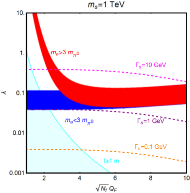
Figure 3: Colored contours representing the different values of $\Gamma_{s}$ in the bi-dimensional plane $(\sqrt{N_{f}}Q_{F},\lambda)$ corresponding to $2$ fb $\lesssim\sigma_{4\gamma}\lesssim 6$ fb for $m_{s}=1\,\mbox{TeV}$ with $m_{a}<3m_{\pi^{0}}$ (blue colored contour) and $m_{a}>3m_{\pi^{0}}$ (red colored contour). The cyan colored region in the left, where the pseudoscalar decays beyond 1 m, is excluded.

A sketch of the aforesaid scenario is depicted in figure 3. Keeping $m_{s}$ fixed at 1 TeV, we can see from figure 3 that in the $m_{a}<3m_{\pi^{0}}$ case, a sizable production cross-section can be obtained, compatible with $l\raise 1.29167pt\hbox{$\;<$\kern-7.5pt\raise-4.73611pt\hbox{$\sim\;$}}1\,\mbox{m}$, only for $Q_{F}\gtrsim 4$ (or with a very high family number $N_{f}$). The variation of $l$ with $\sqrt{N_{f}}Q_{F}$ and $\lambda$ is consistent with eq. (2.7) which predicts smaller pseudoscalar decay lengths for increasing $\sqrt{N_{f}}Q_{F}$ and $\lambda$ values. On the contrary, the limit on the decay length does not affect the $m_{a}>3m_{\pi^{0}}$ scenario since one has to consider much larger values of $\lambda$ to compensate (i.e., through Br$(s\to aa)$) the suppression from $\mathrm{Br}(a\rightarrow\gamma\gamma)^{2}$ as long as $Q_{F}\leq 4$. We notice that for $Q_{F}\gtrsim 4$ the predictions for the two regimes, $m_{a}>3m_{\pi^{0}}$ and $m_{a}<3m_{\pi^{0}}$, tend to coincide since for such large $Q_{F}$ values, the quantity Br$(a\to\gamma\gamma)$ remains $\approx 1$ irrespective of the fact whether the hadronic channel is kinematically accessible or not.

It is interesting to note that for this model, due to its dynamical construction, a direct link between the width of the resonance and the multi-photon production cross-sections $(\sigma_{2\gamma},\,\sigma_{4\gamma})$ appears feasible. Hence, given this model, any future measurement of an excess by the ATLAS or CMS group could be used to estimate the total width as given by eq. (2.9) and eq. (2.3). We note in passing that the results derived up to now are substantially insensitive to the mass of the new fermions. However, as will be discussed in the next section, the mass $m_{F}$ plays a very relevant role once the UV consistency of the theory is taken into account and this will translate, in turn, into stringent constraints on the low-energy phenomenology.

3 The ultra-violet regime

As already stated in the introduction, the SM model extensions with new fermionic states, having sizable $(\mathcal{O}(1))$ couplings with the new scalar (pseudoscalar) fields, face potentially strong constraints from the RGE evolution of the different relevant parameters of the theory. For example, modified $\beta$ functions of the SM gauge couplings, in the presence of new BSM states, can possibly lead to a Landau pole rather fast. As already argued in ref. [51], the parameter which is highly sensitive to radiative corrections is the quartic coupling $\lambda$, whose $\beta$ function contains a negative contribution proportional to $y_{F}^{4}$. Hence, a starting value of $y_{F}\sim\mathcal{O}(1)$ or higher, as typically required for having sizable diphoton cross-sections, will drive the quartic coupling towards negative values at a rather low energy scale. Thus, the vacuum of the theory gets destabilized unless additional and opposite signed contributions are added at the cost of incorporating more new bosonic degrees of freedom.

In our dynamical framework, the Yukawa couplings of the new fermions directly depend on their masses, the mass of the scalar resonance $m_{s}$ as well as the quartic coupling $\lambda$ : $y_{F}=2\sqrt{\lambda}m_{F}/m_{s}$. Parameters $m_{s}$ and $\lambda$ being responsible for the diphoton production cross-section, it appears feasible to connect the experimental limits on the diphoton production cross-section and the requirement of the UV consistency of the theory, depending on the mass of the vector-like fermions.

Indeed, the relevant RGE equations for the studied dynamical model are given by:

$$\frac{d{y}_{F}}{d\ln\mu}=\beta_{y}=\frac{1}{16\pi^{2}}\left((1+6N_{f}){y}_{F}^{3}-24\pi{y}_{F}\alpha_{1}Q^{2}_{F}-32\pi{y}_{F}\alpha_{s}\right),$$

$$\frac{d\lambda}{d\ln\mu}=\beta_{\lambda}=\frac{1}{16\pi^{2}}(20\lambda^{2}-12N_{f}y_{F}^{4}+24\lambda N_{f}y_{F}^{2}),$$ (3.1)

where $\alpha_{1}=g_{1}^{2}/4\pi$ and $\alpha_{s}=g_{3}^{2}/4\pi$. At a energy scale $\mu\geq m_{F}$, the gauge couplings $\alpha_{1},\alpha_{s}$ are given by:

$$\alpha_{1}(\mu)={\left[\frac{1}{\alpha_{1,\rm SM}(m_{F})}-\frac{b_{1}^{\rm SM}+\Delta b_{1}}{2\pi}\ln\left(\frac{\mu}{m_{F}}\right)\right]}^{-1},$$

$$\alpha_{s}(\mu)={\left[\frac{1}{\alpha_{s,\rm SM}(m_{F})}-\frac{b_{3}^{\rm SM}+\Delta b_{3}}{2\pi}\ln\left(\frac{\mu}{m_{F}}\right)\right]}^{-1},$$ (3.2)

where $(b_{1}^{\rm SM},b_{3}^{\rm SM},\Delta b_{1},\Delta b_{3})=({41}/{6},-7,8N_{f}Q_{F}^{2},{4}N_{f}/3)$ . A Landau pole is considered when at a given energy scale $\mu,$ $\alpha_{1}(\mu),\,\alpha_{s}(\mu)=1$. Given the chosen gauge quantum number assignments of the new fermions, the coupling $\alpha_{1}$ is the one which might most likely encounter a Landau pole first. However, for $N_{f}=1$ and $Q_{F}\leq 2$, as considered for most of our analysis (see next section for clarification), the Landau pole of $\alpha_{1}$ lies at rather high scales, above $10^{9}\,\mbox{GeV}$. As a consequence, the constraints derived from Renormalization Group (RG) evolution apply mainly for the parameters $y_{F}$ and $\lambda$, as described by eq .(3.1). The quartic coupling $\lambda$, as also discussed in ref. [51], is very sensitive to the radiative corrections. A simple analytical estimate can then be obtained as suggested in ref. [51] by inspecting the ratio $|\beta_{\lambda}/\lambda|$. A value of this ratio greater than one would imply a very fast variation of $\lambda$ with energy scale, triggered by the radiative corrections, such that the theory would show a pathological behavior at rather low energy scales, unless suitably supplemented with new contributions. In particular we notice that $\beta_{\lambda}$ contains a negative contribution scaling as $y_{F}^{4}$ with a rather large coefficient. Hence, for a high enough starting value of $y_{F}$ (in this case $\beta_{y}>0$ and so $y_{F}$ would increase with the energy scale) the quartic coupling $\lambda$ would be driven towards a negative value, destabilizing the vacuum of the theory. By approximating $\beta_{\lambda}\approx-\frac{12}{16\pi^{2}}N_{f}y_{F}^{4}$ from eq. (3.1) and substituting $y_{F}=2\sqrt{\lambda}\frac{m_{F}}{m_{s}}$ one obtains:

$$\left|\frac{\beta_{\lambda}}{\lambda}\right|\simeq\frac{12N_{f}}{\pi^{2}}\lambda\left(\frac{m_{F}}{m_{s}}\right)^{4},$$ (3.3)

which gives $|\beta_{\lambda}/\lambda|\simeq 1.2\lambda\left(\frac{m_{F}}{m_{s}}\right)^{4}$ for $N_{f}=1$.

Now one can trade $\lambda$ with $\sigma_{4\gamma}$ to translate eq. (3.3) into an upper bound for the diphoton cross-section. Considering eq. (2.3) for example with $N_{f}=1$, one obtains:

$$\sigma_{4\gamma}\lesssim 0.83\,{\mbox{fb}}\,\,Q_{F}^{8}\left(\frac{m_{s}}{m_{F}}\right)^{4}\left(\frac{I_{GG}(m_{s}/\sqrt{s})}{2000}\right).$$ (3.4)

For $N_{f}=1$ and $Q_{F}=2$, one obtains $\sigma_{4\gamma}\lesssim 0.5$ fb ($0.07$ fb) for $m_{F}=3$ TeV (5 TeV) in the case of a $m_{s}=1$ TeV resonance, which are well below the current experimental sensitivity [11, 12]. This behavior can be easily understood by the fact that larger $m_{F}$ (i.e., larger $y_{F}$) should be compensated with smaller $\lambda$ to maintain $|\beta_{\lambda}/\lambda|$ well behaved, i.e., $<1$ (see eq. (3.3)). In other words, an observation of a signal in the near future would imply that the mass of the new fermions should not be too far from the one of the resonance and their future detection are well envisaged.

For numerical studies, we have performed a more systematic investigation by solving the relevant RGEs, i.e., eq. (3.1) in combination with eq. (3).

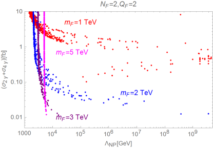
Figure 4: The collective production cross-section for a diphoton-like signal as a function of the scale $\Lambda_{NP}$ where the quartic coupling becomes negative. Here, we consider $N_{f}=1,Q_{F}=2$ and the different $m_{F}$ values are mentioned in the plot.

The result of our numerical study is illustrated by figure 4. which represents the scan on the parameters space $\lambda,m_{s}$ and $m_{a}$ (see section 5 for details) for different values for $m_{F}$, namely $1,2,3$ and $5$ TeV with $N_{f}=1,\,Q_{F}=2$. Figure 4 depicted the collective value of diphoton production cross-section, i.e., $\sigma_{2\gamma}+\sigma_{4\gamma}$ as a function of the scale $\Lambda_{NP}$ where the quartic coupling $\lambda$ becomes negative. We can clearly see in the figure that for $m_{F}\leq 2$ TeV it is possible to have sizable diphoton production cross-section up to $\Lambda_{\rm NP}\sim O(10^{9}\,\mbox{GeV})$, a value also corresponding to the Landau pole of $\alpha_{1}$. On the contrary, all the configurations with $m_{F}=3-5\,\mbox{TeV}$ feature $\Lambda_{\rm NP}\sim m_{F}$. This implies that for these masses new degrees of freedom should already be introduced at scales equal or below $m_{F}$ to secure a well-behaved theory up to some energy scale much larger than the involved mass spectrum.

4 Introducing a dark sector

It is rather straightforward to embed Dark Matter (DM) candidates in this dynamical framework by adding extra fermions charged only under the new $U(1)$ symmetry but singlet under the SM gauge group. In this paper we will consider the case of a Majorana fermion $\chi$ described by the following Lagrangian:

$${\cal L}_{\chi}=\frac{1}{2}i\bar{\chi}\gamma^{\mu}\partial_{\mu}\chi-y_{\chi}\Phi\bar{\chi}^{c}\chi+\text{h.c.}\,\,\,\,=\frac{1}{2}i\bar{\chi}\gamma^{\mu}\partial_{\mu}\chi-\frac{y_{\chi}}{\sqrt{2}}s\bar{\chi}^{c}\chi-i\frac{y_{\chi}}{\sqrt{2}}a\bar{\chi}^{c}\gamma^{5}\chi.$$ (4.1)

Similar to the new BSM fermions, producing interactions among $\Phi$ with photons and gluons, the DM Yukawa coupling $y_{\chi}$ can also be expressed as the function of $\lambda$, $m_{s}$ and DM mass such that the DM mass $m_{\chi}$ appears as the only new additional parameter. As already shown in ref. [33], that the presence of DM does not influence the prediction of 4-photon production cross-section since, when kinematically allowed, invisible decay processes like $s\rightarrow\chi\chi$ or even $a\rightarrow\chi\chi$ would feature a suppressed branching fraction.

In general a contribution from DM Yukawa $y_{\chi}$ should also be included in the RGE system, eq. (3.1). However, being singlet under $SU(3)_{C}$, the related coefficients would be smaller than $y_{F}$ by a factor of three. Moreover, we always assume, throughout this work, $m_{\chi}\leq m_{F}$ so that $y_{\chi}$ is always reduced with respect to $y_{F}$. For this reason the impact of $y_{\chi}$ on the RGE behavior of the theory can assumed to be marginal and thus, not considered in our analyses.

DM phenomenology: For a dark matter candidate $\chi$ heavier than the pseudoscalar $a$, the correct relic density $\Omega h^{2}\simeq 0.12$ [53, 54] can be achieved through a classical freeze out with a thermally averaged pair annihilation cross-section $\langle\sigma v\rangle\sim 3\times 10^{-26}\,{\mbox{cm}}^{3}{\mbox{s}}^{-1}$. Regarding the annihilation cross-section, we can achieve good analytical approximations in the two limiting cases: $m_{a}<m_{\chi}<m_{s}/2$ and $m_{\chi}>m_{s}/2$. Notice that we will always assume $m_{\chi}<m_{F}$ so that the annihilation process $\chi\chi\rightarrow FF$ remains kinematically forbidden.

In the light DM regime ($m_{\chi}\lesssim m_{s}/2$) the main annihilation channels are $\chi\chi\rightarrow gg$ and $\chi\chi\rightarrow\gamma\gamma$, mostly determined by the s-channel exchange of the pseudoscalar state $a$, as well as $\chi\chi\rightarrow aa$. The corresponding cross-sections can be approximated, using a velocity expansion, as:

$$\langle\sigma v\rangle_{\rm gg}=\frac{16\lambda^{2}|\widetilde{C}_{\rm GG}|^{2}m_{\chi}^{2}}{\pi m_{s}^{4}}\approx 1.1\times 10^{-32}\,{\mbox{cm}}^{3}{\mbox{s}}^{-1}{\left(\frac{\lambda}{0.01}\right)}^{2}{\left(\frac{m_{\chi}}{100\,\mbox{GeV}}\right)}^{2}{\left(\frac{750\,\mbox{GeV}}{m_{s}}\right)}^{4}N^{2}_{f},$$ (4.2)

$$\langle\sigma v\rangle_{\rm\gamma\gamma}=\frac{2\lambda^{2}c_{W}^{4}|\widetilde{C}_{\rm BB}|^{2}m_{\chi}^{2}}{\pi m_{s}^{4}}\approx 2.1\times 10^{-34}\,{\mbox{cm}}^{3}{\mbox{s}}^{-1}Q_{F}^{4}{\left(\frac{\lambda}{0.01}\right)}^{2}{\left(\frac{m_{\chi}}{100\,\mbox{GeV}}\right)}^{2}{\left(\frac{750\,\mbox{GeV}}{m_{s}}\right)}^{4}N^{2}_{f},$$ (4.3)

$$\langle\sigma v\rangle_{aa}=\frac{9m_{\chi}^{2}\lambda^{2}}{384\pi m_{s}^{4}}v^{2}\approx 2.7\times 10^{-32}\,{\mbox{cm}}^{3}{\mbox{s}}^{-1}{\left(\frac{\lambda}{0.01}\right)}^{2}{\left(\frac{m_{\chi}}{100\,\mbox{GeV}}\right)}^{2}{\left(\frac{750\,\mbox{GeV}}{m_{s}}\right)}^{4}.$$ (4.4)

It is evident that the annihilation cross-sections into the SM gauge boson pairs are s-wave dominated, i.e., do not depend on the velocity $v$ while the annihilation into a pseudoscalar pair is p-wave suppressed. In the scenario when the DM annihilation is dominated by the SM final states, the s-wave nature of the cross-section would imply that DM annihilations are efficient also at the present times and would be capable of generating an indirect detection signal, detectable with the ongoing experiments. We notice, in particular, that for $Q_{F}\gtrsim 2$, the annihilation cross-section into $\gamma\gamma$ tends to be very close to the other ones. This possibility is in strong tension with the limits set by FERMI [55] gamma-ray line searches, being as strong as $10^{-(29\div 30)}$ for $m_{\chi}\raise 1.29167pt\hbox{$\;<$\kern-7.5pt\raise-4.73611pt\hbox{$\sim\;$}}100$ GeV.

When the DM mass is well above $m_{s}/2$, $\langle\sigma v\rangle$ is instead dominated by the process $\chi\chi\rightarrow sa$ whose cross-section can be estimated as:

$$\langle\sigma v\rangle_{sa}=\frac{\lambda^{2}}{8\pi}\frac{m_{\chi}^{2}}{m_{s}^{4}}\approx 1.2\times 10^{-29}\,{\mbox{cm}}^{3}{\mbox{s}}^{-1}{\left(\frac{\lambda}{0.01}\right)}^{2}{\left(\frac{m_{\chi}}{500\,\mbox{GeV}}\right)}^{2}{\left(\frac{750\,\mbox{GeV}}{m_{s}}\right)}^{4}.$$ (4.5)

This annihilation channel features a s-wave cross-section. However, the indirect signal is more peculiar since it would be represented by (wide) $\gamma$-ray boxes which can be investigated, in the near future, by the CTA experiment [56, 57, 33].

Regarding the other dark matter search strategies, e.g., LHC signals like monojets [58, 59] are suppressed by the already mentioned low invisible branching fraction of the scalar resonance. Direct detection signals are similarly below the current experimental sensitivity [39] but can be within the reach of upcoming future detectors [60, 61].

As evident from the aforesaid expressions that the DM annihilation cross-section strongly depends on the parameters $\lambda$ and $m_{s}$, relevant for determining LHC observables like, $\sigma_{4\gamma}+\sigma_{2\gamma}$ and $\Gamma_{s}$, as well as the theoretical consistency of a model framework. As a consequence, the requirement of the correct relic density might influence the predictions of the diphoton cross-section. Similarly, requiring a theoretically consistent framework up to a given energy scale $\Lambda_{\rm NP}$ might set limit on the viable parameter space for the DM.

By combining the aforementioned expressions of the pair annihilation cross-sections with eq. (2.9) and eq. (2.3), one can obtain the following approximate predictions for the 4-photon production cross-section:

$$\sigma_{4\gamma}\approx 3.4\,\mbox{pb}\,N^{2}_{f}\left(\frac{I_{\rm GG}(m_{s}/\sqrt{s})}{2000}\right){\left(\frac{\langle\sigma v\rangle_{aa}}{3\times 10^{-26}\,{\mbox{cm}}^{3}{\mbox{s}}^{-1}}\right)}^{1/2}\left(\frac{100\,\mbox{GeV}}{m_{\chi}}\right){\left(\frac{m_{s}}{1\,\mbox{TeV}}\right)}^{2},$$

$$\hskip 278.83708pt\left[\rm{for}~{}m_{a}<3m_{\pi^{0}},m_{\chi}<m_{s}/2\right],$$

$$\sigma_{4\gamma}\approx 1.3\,\mbox{fb }\,N^{2}_{f}Q_{F}^{8}\left(\frac{I_{\rm GG}(m_{s}/\sqrt{s})}{2000}\right){\left(\frac{\langle\sigma v\rangle_{aa}}{3\times 10^{-26}\,{\mbox{cm}}^{3}{\mbox{s}}^{-1}}\right)}^{1/2}\left(\frac{100\,\mbox{GeV}}{m_{\chi}}\right){\left(\frac{m_{s}}{1\,\mbox{TeV}}\right)}^{2},$$

$$\hskip 278.83708pt\left[\rm{for}~{}m_{a}>3m_{\pi^{0}},m_{\chi}<m_{s}/2\right],$$

$$\sigma_{4\gamma}\approx 163\,\mbox{fb}\,N^{2}_{f}\left(\frac{I_{\rm GG}(m_{s}/\sqrt{s})}{2000}\right){\left(\frac{\langle\sigma v\rangle_{sa}}{3\times 10^{-26}\,{\mbox{cm}}^{3}{\mbox{s}}^{-1}}\right)}^{1/2}\left(\frac{500\,\mbox{GeV}}{m_{\chi}}\right){\left(\frac{m_{s}}{1\,\mbox{TeV}}\right)}^{2},$$

$$\hskip 278.83708pt\left[\rm{for}~{}m_{a}<3m_{\pi^{0}},m_{\chi}>m_{s}/2\right],$$

$$\sigma_{4\gamma}\approx 0.06\,\mbox{fb }\,N^{2}_{f}Q_{F}^{8}\left(\frac{I_{\rm GG}(m_{s}/\sqrt{s})}{2000}\right){\left(\frac{\langle\sigma v\rangle_{sa}}{3\times 10^{-26}\,{\mbox{cm}}^{3}{\mbox{s}}^{-1}}\right)}^{1/2}\left(\frac{500\,\mbox{GeV}}{m_{\chi}}\right){\left(\frac{m_{s}}{1\,\mbox{TeV}}\right)}^{2},$$

$$\hskip 278.83708pt\left[\rm{for}~{}m_{a}>3m_{\pi^{0}},m_{\chi}>m_{s}/2\right].$$

We can see that in the $m_{a}<3m_{\pi^{0}}$ scenario, the cross-section favored by the correct relic density largely exceeds, almost by two orders of magnitude, the current experimental limits for $m_{s}$ of the order of a TeV. On the contrary, for $m_{a}>3m_{\pi^{0}}$ scenario it is possible to obtain the correct DM relic density compatible with an observable collimated photon signal for $Q_{F}\lesssim 2$. However, as already mentioned, for $Q_{F}=2$, in the low DM region the $\gamma\gamma$ final state channel has a too high branching fraction and thus, results in tension with limits from the indirect detection. We further remark that, given the $Q_{F}^{8}$ dependence of the second and fourth expression of eq. (4), the combination of the correct DM relic density and the LHC diphoton production cross-section limits imposes very stringent constraint for $Q_{F}\lesssim 2$.

Figure 5: Isocontour (red colored) of the correct DM relic density, for $m_{s}=1\,\mbox{TeV},\,N_{f}=1,\,Q_{F}=2$, in the $(\lambda,m_{\chi})$ plane. The orange colored region is excluded by the indirect detection experiments while the dashed blue line represents the projected LZ sensitivity [61]. The magenta and purple colored bands represent the range $4\pm 2\,\mbox{fb}$ for the collimated diphoton production cross-section in the $m_{a}<3m_{\pi^{0}}$ and $m_{a}>3m_{\pi^{0}}$ scenarios, respectively.

We have verified all the analytical estimates given in this section by numerically computing the thermally averaged DM pair annihilation cross-section in order to account also the pole region $m_{\chi}\simeq m_{s}/2$ properly. In figure (5) we show an isocontour of the correct DM relic density in the bi-dimensional plane $(\lambda,m_{\chi})$ for $N_{f}=1,\,Q_{F}=2$ and $m_{s}=1$ TeV. This contour is confronted with the prediction of a collimated diphoton cross-section, within the range of $4\pm 2\,\mbox{fb}$, for the two cases: $m_{a}>3m_{\pi^{0}}$ and $m_{a}<3m_{\pi^{0}}$. For the latter, as a consequence of the very low values of $\lambda$ imposed by the diphoton production cross-section, the only region compatible with the collider limits is the pole region $m_{\chi}\sim m_{s}/2$. On the contrary, in the $m_{a}>3m_{\pi^{0}}$ scenario, the suppression factor from $\mathrm{Br}(a\rightarrow\gamma\gamma)^{2}$ should be compensated by a higher value of $\lambda$ which allows a fit of the DM relic density, through the annihilation into $sa$ final state, for DM masses of the order of 600 GeV. The light DM region, being excluded by limits from the Indirect Detection experiments, remains inaccessible.

It can be easily noticed that we have a more constrained scenario with respect to the one depicted in ref. [33] with the effective field theory approach. This is because, in the dynamical construction the $C_{\rm GG}$ and $C_{\rm BB}$ parameters as well as their relative hierarchy are not free, but substantially guided by the quantum number assignments of the new fermions. In particular their values are always above $O(10^{-2})$, greater than the ones typically quoted in ref. [33].

5 Summary and discussion

In the previous sections we have described, through some examples, the relation between the collider limits/predictions and the theoretical consistency of the studied dynamical framework and their collective impact on the DM phenomenology. In this summary we illustrate the results of a systematic numerical study based on a scan involving the relevant free parameters of the model. The chosen parameters are the four masses $m_{s},\,m_{a},\,m_{\chi},\,m_{F}$, the electric charge $Q_{F}$ and the quartic coupling $\lambda$. The latter parameter, through eq. (2.9), eq. (2.3) and eq. (2.12), can be traded with a physical observable, i.e., the total diphoton production cross-section $\sigma_{2\gamma}+\sigma_{4\gamma}$. This collective production cross-section is varied in the span of $10\,\mbox{fb}$, i.e., of the order of the present experimental bounds, to $10^{-2}\,\mbox{fb}$, which would correspond to the observation of $O(1)$ events at the maximal expected luminosity for LHC run-II, $O(100\,{\mbox{fb}}^{-1})$. The four parameters $m_{s},m_{a},m_{\chi},\sigma_{2\gamma}+\sigma_{4\gamma}$, together with $Q_{F}$, determine the other experimental observables, i.e., the total width of the scalar resonance and the interaction rates of the DM and finally, including $m_{F}$, the energy scale $\Lambda_{\rm NP}$ at which the theory should be UV completed.

Choosing one family of the new BSM fermion, i.e., $N_{f}=1$, we have varied the three masses $m_{s}$, $m_{a}$, $m_{\chi}$ and $\sigma_{2\gamma}+\sigma_{4\gamma}$ in the following ranges:

$$m_{s}\in\left[200,2000\right]\,\mbox{GeV},$$

$$m_{a}\in\left[0.2,2\right]\,\mbox{GeV},$$

$$m_{\chi}\in\left[100,1000\right]\,\mbox{GeV},$$

$$\sigma_{2\gamma}+\sigma_{4\gamma}\in\left[10^{-2},10\right]\,\mbox{fb}.$$ (5.1)

The scan has been repeated for five discrete values of $m_{F}$, namely $1,2,3$ and $5\,\mbox{TeV}$ and for $Q_{F}=1$ and $2$. For each set of the considered parameters we have computed the LHC and DM observables as well as the value of $\Lambda_{\rm NP}$. Further, for each model configuration we have imposed the constraints of correct DM relic density, observational DM limits, a pseudoscalar decay length $l\leq 1\,\mbox{m}$ and finally, $\Gamma_{s}/m_{s}\leq 10\%$. Furthermore, we consider $m_{F}\geq m_{s}$ and $y_{F}<\sqrt{4\pi}$ in all our analyses.

A first outcome of this scan has already been depicted in figure 4, which shows that for $m_{F}=3$ and $5$ TeV it is extremely difficult, or even impossible, to achieve observable diphoton production cross-section in a theoretically consistent way. Thus, we will focus our discussion on the results of the cases $m_{F}=1$ and $2\,\mbox{TeV}$.

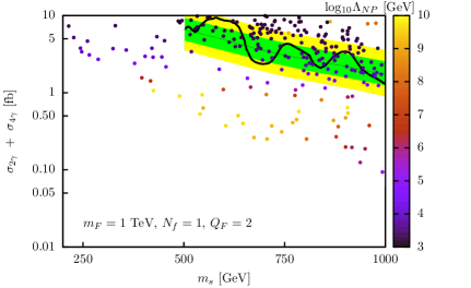
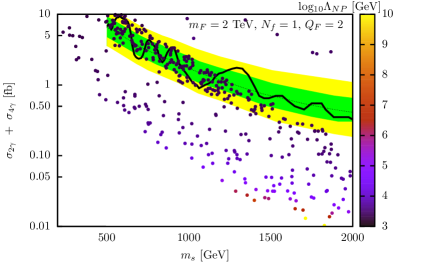
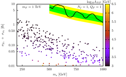
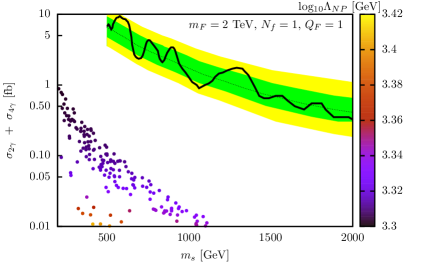
Figure 6: Distribution of the model configurations in the $(\sigma_{2\gamma}+\sigma_{4\gamma},m_{s})$ plane. The corresponding $m_{F}$ and $Q_{F}$ values are given in the plots. The color coding represents the different values of $\Lambda_{\rm NP}$. The experimental data (represented with the familiar yellow-green plot) used in these plots corresponds to 16.2 fb^-1 of data at $\sqrt{\bf{s}}$=13 TeV + 19.7 fb^-1 of data at $\sqrt{\bf{s}}$=8 TeV, with $\Gamma_{s}/m_{s}=5.6\%$, from the latest CMS result [62].

We have plotted in figure 6 the prediction of a diphoton signal at the LHC, i.e., $\sigma_{2\gamma}+\sigma_{4\gamma}$, as a function of the mass of the scalar resonance, where each of the model configurations are tested against the list of constraints mentioned above. The associated color coding represents the value of $\Lambda_{\rm NP}$ for a given model configuration. The predictions, estimated with this model, are compared with the limits (plotted with the familiar yellow-green style) recently reported by the CMS group [12]. From figure 6 it is apparent, that for $Q_{F}=2$ (top row) most of the points lie within the current experimental sensitivity or slightly below, especially when $\Lambda_{\rm NP}$ is large. The region with large $\Lambda_{\rm NP}$, as expected from the UV behavior of the theory (see section 3), shifts towards higher $m_{s}$ values for increasing $m_{F}$ and produces an anticipated reduction in $\sigma_{2\gamma}+\sigma_{4\gamma}$.

Further, the configurations lying within the 1-2$\sigma$ bands of the current experimental observation typically appear with the lower values of $\Lambda_{\rm NP}$. This is because, for a given value of $m_{s}$, a higher production cross-section implies higher values of $\lambda$ (see subsection 2.3) and hence, a higher starting values of $y_{F}$ since $y_{F}\propto\sqrt{\lambda}$. This, in turn would produce a more negative $\beta_{\lambda}/\lambda$, forcing $\lambda$ to turn negative at a lower $\Lambda_{\rm NP}$. Relatively well UV behaved configurations lie below the current experimental limits and are expected to be probed in the near future.

For $Q_{F}=1$, on the contrary, all the points lie well below the current experimental sensitivity. This is in agreement with eq. (4) which suggests that the DM relic density favors very small, even below $10^{-2}\,\mbox{fb}$ LHC cross-sections. We also notice that in the $Q_{F}=1$ case (bottom row of figure 6), a much stronger requirement exists on the value of $m_{F}$ from the UV behavior of the theory. We observe that basically all the points, for $m_{F}=2\,\mbox{TeV}$, feature $\Lambda_{\rm NP}\simeq m_{F}$ (bottom row, right) and in the case of $m_{F}=1\,\mbox{TeV}$, one gets $\Lambda_{\rm NP}$ not exceeding $10^{6}\,\mbox{GeV}$ (bottom row, left). This arises due to the $Q_{F}^{8}$ dependence of the 4-photon production cross-section (we remind that the regime $m_{a}<3m_{\pi^{0}}$, for which the cross-section does not depend on $Q_{F}$, is largely incompatible with the correct relic density) which implies larger values of $\lambda$ for obtaining the same value of the production cross-section (see also figure 3). The large $\lambda$ values would lead to a more problematic UV behavior of the model.

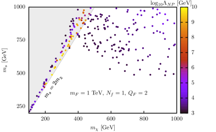
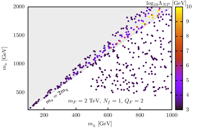
Figure 7: Distribution of the model configurations in the $(m_{\chi},m_{s})$ plane for the different $m_{F}$, $Q_{F}$ values, mentioned in the plots. The gray colored region represents the $m_{\chi}\leq m_{s}/2$ scenario. The color coding represents the different values of $\Lambda_{\rm NP}$.

Finally, just for the $Q_{F}=2$ scenario, we have shown in figure 7 the distribution of points in the $(m_{\chi},m_{s})$ plane to highlight the regions of the parameter space favored by the correct DM relic density. Once again, as suggested by eq. (4), we notice that the region corresponding to $m_{\chi}<m_{s}/2$ (gray colored) is substantially empty. Regarding the value of $\Lambda_{\rm NP}$, we observe that the maximal values lie in the resonance region $m_{\chi}\simeq m_{s}/2$. This happens since the enhancement of the DM annihilation cross-section in this regime allows to fit the correct relic density for lower values of $\lambda$ which guarantee a better UV behavior of the theory.

6 Conclusion

In this article we have presented a model where the SM is extended by a SM gauge singlet complex scalar field $\Phi$, a set of new BSM fermions charged also under the SM gauge group and a fermionic DM candidate, singlet under the SM gauge charges but charged under the new global $U(1)$ symmetry associated with the $\Phi$ field. All the masses in this theory, except for the pseudo Goldstone $a$, are dynamically generated from spontaneous breaking of the associated $U(1)$ symmetry so that the theory has only one fundamental scale, represented by the scale of spontaneous symmetry breaking.

The typical LHC signature of this model is the production of pairs of collimated photons produced from the decay of a pair of pseudo Goldstone bosons $a$ (the imaginary component of $\Phi$), originated from a scalar resonance $s$ (the real component of $\Phi$) while other possible processes, like dijets, $Z\gamma$ and $ZZ$ productions, have rather suppressed rates. The couplings responsible for the collective diphoton, i.e., $2\gamma+4\gamma$, production are induced by the new BSM fermions at the one-loop level. However, given the dynamical structure of the model, the couplings are practically independent of the BSM fermion masses, so that the cross-section depends mainly on $m_{s}$, the quartic coupling $\lambda$, the number of BSM fermion families $N_{f}$ and on their electric charges $Q_{F}$. As a consequence there exists direct correlation between the collective diphoton production cross-section, i.e., $\sigma_{2\gamma}+\sigma_{4\gamma}$, and the total decay width $\Gamma_{s}$ of the resonance.

The presence of colored and electrically charged new BSM fermions has a strong impact on the UV behavior of the theory. Indeed the quartic coupling $\lambda$ can be driven rather efficiently towards negative values at a energy scale $\Lambda_{\rm NP}$ in the vicinity of $m_{F}$ such that a further completion of the theory should be invoked at the energy scale $\Lambda_{\rm NP}$. Again, the dynamical structure of the model gives a tight relation between the value of $\Lambda_{\rm NP}$ and the experimentally measurable diphoton production cross-section.

We have shown that for masses of the new BSM fermions not exceeding 2 TeV, having electric charge $Q_{F}=1$ or $2$, the considered framework is theoretically consistent up to some energy scale $\Lambda_{\rm NP}\sim 2.5~{}{\rm TeV}~{}(10^{10}~{}{\rm GeV})$ for $Q_{F}=1~{}(2)$, starting from $\gtrsim m_{F}$. Thus, at least part of the $\Lambda_{\rm NP}$ remains within the reach of ongoing and upcoming collider experiments and, at the same time can produce an observable signal. It is possible, in addition, to achieve a DM candidate with the correct relic density without conflicting with the existing search results. The DM sector for this model is capable of producing signals in the indirect detection experiments which are expected to be probed in the near future.

Appendix A Loop induced coefficients

For completeness, in this appendix we present the detailed expressions for the loop induced coefficients $C_{\rm BB}$, $C_{\rm GG}$, $\widetilde{C}_{\rm BB}$ and $\widetilde{C}_{\rm GG}$.

Given the effective Lagrangian:

$$-{\cal L_{\mathrm{eff}}}\supset k_{GG}sG^{\alpha}_{\mu\nu}G^{\mu\nu}_{\alpha}+k_{BB}sB_{\mu\nu}B^{\mu\nu}+\tilde{k}_{GG}aG^{a}_{\mu\nu}\widetilde{G}^{\mu\nu}_{a}+\tilde{k}_{BB}aB_{\mu\nu}\widetilde{B}^{\mu\nu},$$ (A.1)

its dimension-full coefficients, when they are originated from the one-loop triangle diagrams involving new fermionic states of masses $m_{F_{\alpha}}$, can be written as [20]:

$$k_{GG}=\frac{\alpha_{s}}{8\pi}\left(\sum_{\alpha}d_{\alpha}^{(2)}C_{\alpha}^{(3)}\frac{1}{\sqrt{2}}\frac{y_{F_{\alpha}}}{m_{F_{\alpha}}}f_{1/2}(\tau_{\alpha})\right),$$ (A.2)

$$k_{BB}=\frac{\alpha_{\text{em}}}{8\pi}\frac{1}{c_{W}^{2}}\left(\sum_{\alpha}(d_{\alpha}^{(3)}C_{\alpha}^{(2)}+d_{\alpha}^{(3)}d_{\alpha}^{(2)}Q^{2}_{F_{\alpha}})\frac{1}{\sqrt{2}}\frac{y_{F_{\alpha}}}{m_{F_{\alpha}}}f_{1/2}(\tau_{\alpha})\right),$$ (A.3)

for the scalar and for the pseudoscalar:

$$\tilde{k}_{GG}=\frac{\alpha_{s}}{8\pi}\left(\sum_{\alpha}d_{\alpha}^{(2)}C_{\alpha}^{(3)}\frac{1}{\sqrt{2}}\frac{y_{F_{\alpha}}}{m_{F_{\alpha}}}\tilde{f}_{1/2}(\tau_{\alpha})\right),$$ (A.4)

$$\tilde{k}_{BB}=\frac{\alpha_{\text{em}}}{8\pi}\frac{1}{c_{W}^{2}}\left(\sum_{\alpha}(d_{\alpha}^{(3)}C_{\alpha}^{(2)}+d_{\alpha}^{(3)}d_{\alpha}^{(2)}Q^{2}_{F_{\alpha}})\frac{1}{\sqrt{2}}\frac{y_{F_{\alpha}}}{m_{F_{\alpha}}}\tilde{f}_{1/2}(\tau_{\alpha})\right),$$ (A.5)

where loop induced $f_{1/2}(\tau_{\alpha})$ and ${\tilde{f}}_{1/2}(\tau_{\alpha})$ functions are defined as:

$$f_{1/2}(\tau)=\frac{2(\tau+(\tau-1)f(\tau))}{\tau^{2}},\,\,\,\,\tilde{f}_{1/2}(\tau)=2\frac{f(\tau)}{\tau},$$ (A.6)

with:

$$f(\tau)=\left\{\begin{array}[]{cc}arc\sin^{2}(\sqrt{\tau})&\tau\leq 1\\ -\frac{1}{4}{\left(\log\left[\frac{1+\sqrt{1-1/\tau}}{1-\sqrt{1-1/\tau}}\right]\right)}^{2}&\tau>1,\end{array}\right.$$ (A.7)

and $\tau_{\alpha}$ defined as :

$$\tau_{\alpha}=\frac{m_{s}^{2}}{4m^{2}_{F_{\alpha}}}~{}\mathrm{(for~{}scalar})\,\,\,\rm{and}\,\,\,\tau_{\alpha}=\frac{m_{a}^{2}}{4m^{2}_{F_{\alpha}}}~{}\mathrm{(for~{}pseudoscalar)}.$$ (A.8)

For $SU(N)$ symmetry group we have $(d_{\alpha}^{(N)},C_{\alpha}^{(N)})=(1,0),\,(N,1/2)$ and $(N^{2}-1,N)$ for a singlet, fundamental and adjoint representation, respectively. Since we have considered the addition of mass degenerate fermions with same quantum number assignments, apart from the sign of $Q_{F}$, we can straightforwardly replace $\sum_{\alpha}\rightarrow 2N_{f}$. Furthermore, in our dynamical setup $y_{F}$ and $m_{F}$ are not independent parameters but are related as $y_{F}=2\sqrt{\lambda}({m_{F}}/{m_{s}})$. Thus, apart from the loop functions $f_{1/2}(\tau_{\alpha})$ and ${\tilde{f}}_{1/2}(\tau_{\alpha})$, it is possible to eliminate the $m_{F}$ dependence in $k_{GG},\,k_{BB}$ etc. The coefficients of eq. (2.2) are obtained by setting $k_{VV}(\tilde{k}_{VV})=\frac{\sqrt{\lambda}}{m_{s}}C_{VV}(\widetilde{C}_{VV})$ where $V=B,\,G$.

References

- [1] ATLAS collaboration, Search for resonances decaying to photon pairs in 3.2 fb-1 of collisions at = 13 TeV with the ATLAS detector, ATLAS-CONF-2015-081 (2015) .
- [2] ATLAS collaboration, Search for resonances in diphoton events with the ATLAS detector at = 13 TeV, ATLAS-CONF-2016-018 (2016) .
- [3] CMS collaboration, Search for new physics in high mass diphoton events in proton-proton collisions at 13TeV, CMS-PAS-EXO-15-004 (2015) .
- [4] CMS collaboration, Search for new physics in high mass diphoton events in of proton-proton collisions at and combined interpretation of searches at and , CMS-PAS-EXO-16-018 (2016) .
- [5] S. D. McDermott, P. Meade and H. Ramani, Singlet Scalar Resonances and the Diphoton Excess, Phys. Lett. B755 (2016) 353–357, [1512.05326].
- [6] J. Ellis, S. A. R. Ellis, J. Quevillon, V. Sanz and T. You, On the Interpretation of a Possible GeV Particle Decaying into , JHEP 03 (2016) 176, [1512.05327].
- [7] M. Low, A. Tesi and L.-T. Wang, A pseudoscalar decaying to photon pairs in the early LHC Run 2 data, JHEP 03 (2016) 108, [1512.05328].
- [8] B. Dutta, Y. Gao, T. Ghosh, I. Gogoladze and T. Li, Interpretation of the diphoton excess at CMS and ATLAS, Phys. Rev. D93 (2016) 055032, [1512.05439].
- [9] A. Falkowski, O. Slone and T. Volansky, Phenomenology of a 750 GeV Singlet, JHEP 02 (2016) 152, [1512.05777].
- [10] A. Angelescu, A. Djouadi and G. Moreau, Scenarii for interpretations of the LHC diphoton excess: two Higgs doublets and vector-like quarks and leptons, Phys. Lett. B756 (2016) 126–132, [1512.04921].
- [11] ATLAS collaboration, Search for scalar diphoton resonances with 15.4 fb-1 of data collected at TeV in 2015 and 2016 with the ATLAS detector, ATLAS-CONF-2016-059 (2016) .
- [12] CMS collaboration, Search for resonant production of high mass photon pairs using 12.9 fb-1 of proton-proton collisions at TeV and combined interpretation of searches at 8 and 13 TeV, CMS PAS EXO-16-027 (2016) .
- [13] R. Franceschini, G. F. Giudice, J. F. Kamenik, M. McCullough, A. Pomarol, R. Rattazzi et al., What is the resonance at 750 GeV?, JHEP 03 (2016) 144, [1512.04933].
- [14] J. Gu and Z. Liu, Physics implications of the diphoton excess from the perspective of renormalization group flow, Phys. Rev. D93 (2016) 075006, [1512.07624].
- [15] A. Salvio and A. Mazumdar, Higgs Stability and the 750 GeV Diphoton Excess, Phys. Lett. B755 (2016) 469–474, [1512.08184].
- [16] P. S. B. Dev, R. N. Mohapatra and Y. Zhang, Quark Seesaw, Vectorlike Fermions and Diphoton Excess, JHEP 02 (2016) 186, [1512.08507].
- [17] M. Son and A. Urbano, A new scalar resonance at 750 GeV: Towards a proof of concept in favor of strongly interacting theories, JHEP 05 (2016) 181, [1512.08307].
- [18] E. Bertuzzo, P. A. N. Machado and M. Taoso, Di-Photon excess in the 2HDM: hasting towards the instability and the non-perturbative regime, 1601.07508.
- [19] A. Salvio, F. Staub, A. Strumia and A. Urbano, On the maximal diphoton width, JHEP 03 (2016) 214, [1602.01460].
- [20] K. J. Bae, M. Endo, K. Hamaguchi and T. Moroi, Diphoton Excess and Running Couplings, Phys. Lett. B757 (2016) 493–500, [1602.03653].
- [21] Y. Hamada, H. Kawai, K. Kawana and K. Tsumura, Models of the LHC diphoton excesses valid up to the Planck scale, Phys. Rev. D94 (2016) 014007, [1602.04170].
- [22] A. Bharucha, A. Djouadi and A. Goudelis, Threshold enhancement of diphoton resonances, Phys. Lett. B761 (2016) 8–15, [1603.04464].
- [23] S. Di Chiara, A. Hektor, K. Kannike, L. Marzola and M. Raidal, Large loop-coupling enhancement of a 750 GeV pseudoscalar from a light dark sector, 1603.07263.
- [24] A. Djouadi and A. Pilaftsis, The 750 GeV Diphoton Resonance in the MSSM, 1605.01040.
- [25] L. D. Landau, On the quantum field theory, Niels Bohr and the Development of Physics, ed. W. Pauli (Pergamon Press, London, 1955) (1955) .
- [26] L. Aparicio, A. Azatov, E. Hardy and A. Romanino, Diphotons from Diaxions, JHEP 05 (2016) 077, [1602.00949].
- [27] J. Chang, K. Cheung and C.-T. Lu, Interpreting the 750 GeV diphoton resonance using photon jets in hidden-valley-like models, Phys. Rev. D93 (2016) 075013, [1512.06671].
- [28] U. Ellwanger and C. Hugonie, A 750 GeV Diphoton Signal from a Very Light Pseudoscalar in the NMSSM, JHEP 05 (2016) 114, [1602.03344].
- [29] F. Domingo, S. Heinemeyer, J. S. Kim and K. Rolbiecki, The NMSSM lives: with the 750 GeV diphoton excess, Eur. Phys. J. C76 (2016) 249, [1602.07691].
- [30] M. Badziak, M. Olechowski, S. Pokorski and K. Sakurai, Interpreting 750 GeV Diphoton Excess in Plain NMSSM, Phys. Lett. B760 (2016) 228–235, [1603.02203].
- [31] B. A. Dobrescu, G. L. Landsberg and K. T. Matchev, Higgs boson decays to CP odd scalars at the Tevatron and beyond, Phys. Rev. D63 (2001) 075003, [hep-ph/0005308].
- [32] B. A. Dobrescu and K. T. Matchev, Light axion within the next-to-minimal supersymmetric standard model, JHEP 09 (2000) 031, [hep-ph/0008192].
- [33] G. Arcadi, P. Ghosh, Y. Mambrini and M. Pierre, Re-opening dark matter windows compatible with a diphoton excess, JCAP 1607 (2016) 005, [1603.05601].
- [34] Y. Mambrini, G. Arcadi and A. Djouadi, The LHC diphoton resonance and dark matter, Phys. Lett. B755 (2016) 426–432, [1512.04913].
- [35] M. Backovic, A. Mariotti and D. Redigolo, Di-photon excess illuminates Dark Matter, JHEP 03 (2016) 157, [1512.04917].
- [36] F. D’Eramo, J. de Vries and P. Panci, A 750 GeV Portal: LHC Phenomenology and Dark Matter Candidates, JHEP 05 (2016) 089, [1601.01571].
- [37] E. Dudas, Y. Mambrini and K. A. Olive, Monochromatic neutrinos generated by dark matter and the seesaw mechanism, Phys. Rev. D91 (2015) 075001, [1412.3459].
- [38] E. Dudas, L. Heurtier and Y. Mambrini, Generating X-ray lines from annihilating dark matter, Phys. Rev. D90 (2014) 035002, [1404.1927].
- [39] LUX collaboration, D. S. Akerib et al., Improved Limits on Scattering of Weakly Interacting Massive Particles from Reanalysis of 2013 LUX Data, Phys. Rev. Lett. 116 (2016) 161301, [1512.03506].
- [40] ATLAS collaboration, G. Aad et al., Search for production of vector-like quark pairs and of four top quarks in the lepton-plus-jets final state in collisions at TeV with the ATLAS detector, JHEP 08 (2015) 105, [1505.04306].
- [41] CMS collaboration, V. Khachatryan et al., Search for vector-like charge 2/3 T quarks in proton-proton collisions at sqrt(s) = 8 TeV, Phys. Rev. D93 (2016) 012003, [1509.04177].
- [42] ATLAS collaboration, G. Aad et al., Search for heavy long-lived multi-charged particles in pp collisions at TeV using the ATLAS detector, Eur. Phys. J. C75 (2015) 362, [1504.04188].
- [43] CMS collaboration, V. Khachatryan et al., Search for long-lived charged particles in proton-proton collisions at sqrt(s) = 13 TeV, 1609.08382.
- [44] Particle Data Group collaboration, K. A. Olive et al., Review of Particle Physics, Chin. Phys. C38 (2014) 090001.
- [45] M. Chala, M. Duerr, F. Kahlhoefer and K. Schmidt-Hoberg, Tricking Landau–Yang: How to obtain the diphoton excess from a vector resonance, Phys. Lett. B755 (2016) 145–149, [1512.06833].
- [46] S. Knapen, T. Melia, M. Papucci and K. Zurek, Rays of light from the LHC, Phys. Rev. D93 (2016) 075020, [1512.04928].
- [47] B. Dasgupta, J. Kopp and P. Schwaller, Photons, photon jets, and dark photons at 750 GeV and beyond, Eur. Phys. J. C76 (2016) 277, [1602.04692].
- [48] A. D. Martin, W. J. Stirling, R. S. Thorne and G. Watt, Parton distributions for the LHC, Eur. Phys. J. C63 (2009) 189–285, [0901.0002].
- [49] A. D. Martin, W. J. Stirling, R. S. Thorne and G. Watt, Uncertainties on alpha(S) in global PDF analyses and implications for predicted hadronic cross sections, Eur. Phys. J. C64 (2009) 653–680, [0905.3531].
- [50] A. D. Martin, W. J. Stirling, R. S. Thorne and G. Watt, Heavy-quark mass dependence in global PDF analyses and 3- and 4-flavour parton distributions, Eur. Phys. J. C70 (2010) 51–72, [1007.2624].
- [51] F. Goertz, J. F. Kamenik, A. Katz and M. Nardecchia, Indirect Constraints on the Scalar Di-Photon Resonance at the LHC, JHEP 05 (2016) 187, [1512.08500].
- [52] D. S. M. Alves, J. Galloway, J. T. Ruderman and J. R. Walsh, Running Electroweak Couplings as a Probe of New Physics, JHEP 02 (2015) 007, [1410.6810].
- [53] WMAP collaboration, G. Hinshaw et al., Nine-Year Wilkinson Microwave Anisotropy Probe (WMAP) Observations: Cosmological Parameter Results, Astrophys. J. Suppl. 208 (2013) 19, [1212.5226].
- [54] Planck collaboration, P. A. R. Ade et al., Planck 2013 results. XVI. Cosmological parameters, Astron. Astrophys. 571 (2014) A16, [1303.5076].
- [55] Fermi-LAT collaboration, M. Ackermann et al., Updated search for spectral lines from Galactic dark matter interactions with pass 8 data from the Fermi Large Area Telescope, Phys. Rev. D91 (2015) 122002, [1506.00013].
- [56] A. Ibarra, H. M. Lee, S. López Gehler, W.-I. Park and M. Pato, Gamma-ray boxes from axion-mediated dark matter, JCAP 1305 (2013) 016; 1603 (2016) E01, [1303.6632].
- [57] A. Ibarra, A. S. Lamperstorfer, S. López-Gehler, M. Pato and G. Bertone, On the sensitivity of CTA to gamma-ray boxes from multi-TeV dark matter, JCAP 1509 (2015) 048; 1606 (2016) E02, [1503.06797].
- [58] CMS collaboration, V. Khachatryan et al., Search for dark matter, extra dimensions, and unparticles in monojet events in proton–proton collisions at TeV, Eur. Phys. J. C75 (2015) 235, [1408.3583].
- [59] ATLAS collaboration, G. Aad et al., Search for new phenomena in final states with an energetic jet and large missing transverse momentum in pp collisions at 8 TeV with the ATLAS detector, Eur. Phys. J. C 75 (2015) 299; C 75 (2015) 408, [1502.01518].
- [60] XENON collaboration, E. Aprile et al., Physics reach of the XENON1T dark matter experiment, JCAP 1604 (2016) 027, [1512.07501].
- [61] LZ collaboration, D. N. McKinsey, The LZ dark matter experiment, J. Phys. Conf. Ser. 718 (2016) 042039.
- [62] C. Rovelli. Search for BSM physics in di-photon final states at CMS, in proceedings of the 38th International Conference on High Energy Physics (ICHEP 2016), Chicago, Illinois, U.S.A., August 3–10 2016.