The Next Generation Virgo Cluster Survey (NGVS). XXV. Fiducial panchromatic colors of Virgo core globular clusters and their comparison to model predictions
Abstract
The central region of the Virgo cluster of galaxies contains thousands of globular clusters (GCs), an order of magnitude more than the numbers found in the Local Group. Relics of early star formation epochs in the universe, these GCs also provide ideal targets to test our understanding of the Spectral Energy Distributions (SEDs) of old stellar populations. Based on photometric data from the Next Generation Virgo cluster Survey (NGVS) and its near-infrared counterpart NGVS-IR, we select a robust sample of GCs with excellent photometry and spanning the full range of colors present in the Virgo core. The selection exploits the well defined locus of GCs in the diagram and the fact that the globular clusters are marginally resolved in the images. We show that the GCs define a narrow sequence in 5-dimensional color space, with limited but real dispersion around the mean sequence. The comparison of these SEDs with the predictions of eleven widely used population synthesis models highlights differences between models, and also shows that no single model adequately matches the data in all colors. We discuss possible causes for some of these discrepancies. Forthcoming papers of this series will examine how best to estimate photometric metallicities in this context, and compare the Virgo globular cluster colors with those in other environments.
Subject headings:
galaxies: clusters: individual (Virgo) - galaxies: photometry - galaxies: star clusters: general - galaxies: stellar content1. Introduction
Globular clusters (GCs) are among the most thoroughly studied stellar populations in the sky. Their analysis has helped us understand stellar evolution, and their ages have set essential constraints on cosmological models. Since their formation, at times possibly as remote as the epoch of re-ionization, they have been affected by the numerous physical processes that shaped baryonic structure in the universe, and they have witnessed the dynamical and chemical evolution of their host galaxies (e.g Pota et al. 2013, Carretta et al. 2010).
Historically, the stars bound in clusters have long been described as examples of coeval and chemically uniform stellar populations. This picture has naturally made GCs targets for the validation of population synthesis models (Renzini & Fusi Pecci 1988).
Recent studies of color-magnitude diagrams and stellar surface chemistries in nearby GCs have demonstrated that the historical picture is only an approximation (Bedin et al. 2004, Gratton et al. 2004, Piotto 2007, Goudfrooij et al. 2009, Piotto et al. 2012 or Renzini et al. 2015). Possible processes responsible for internal spreads in stellar properties include self-enrichment, the merging of individual proto-clusters, or the formation of nuclear clusters in galaxies that are subsequently disrupted by tidal fields. Detailed studies of these effects will be best carried out with resolved observations, but the diversity of possible properties of GCs can also be tested, out to much larger distances, with precise integrated multi-band photometry.
Over time, several studies have targeted nearby galaxies, producing catalogs of integrated photometry for GC samples. To mention just a few: the McMaster catalog of Harris (1996, and references therein) collects UBVRI colors of several dozen teams for 157 GCs of the Milky Way; the work of Searle et al. (1980) on the Magellanic Clouds has provided the uvgr colors of 61 star clusters, on which the popular (but now somewhat outdated) SWB (Searle Wilkinson Bagnuolo) classification was based; the Revised Bologna Catalog (Galleti et al., 2004) lists optical and near-infrared photometry for several hundred globular cluster candidates around M 31, of which however not all have been confirmed by more recent homogeneous surveys (Huxor et al., 2014). Finally, global studies of GC populations as a function of host galaxy properties have yielded optical photometry for samples of a few to a few globular cluster candidates in various environments (e.g. Lotz et al. 2004; Kundu & Whitmore 2001), but typically only for two photometric passbands.
An important result of such surveys was the identification of color subpopulations among GCs, as already suspected by Kinman (1959). In 1985, Zinn showed that two distinct GCs subpopulations coexist in the Galaxy, and linked this to a metallicity bimodality. In the following decades, it was shown that the distribution of blue (metal poor) GCs is mostly associated with the stellar halo of galaxies, while the red (more metal rich) GCs are mostly located in the central regions (e.g Geisler et al. 1996, Côté et al. 2001, Forte et al. 2005, Tamura et al. 2006 or Durrell et al. 2014). Although the shape of the color-metallicity relation remains a matter of debate (Yoon et al. 2006, Blakeslee et al. 2012, Usher et al. 2015), it is now generally accepted that globular clusters are found spread over three orders of magnitude in metallicity, and that their mean metallicities are related to their host galaxy stellar mass or luminosity (e.g Peng et al. 2006).
Large, deep and well resolved surveys are critical for the definition of representative GC samples with limited contamination, and they are progressively becoming available. Targets like the Virgo, Coma or Fornax clusters are now being studied in detail. The path was opened with surveys of the Hubble Space Telescope Advanced Camera for Surveys (HST/ACS), which was used with two bandpasses (F475W and F850LP) to scrutinize galaxies in the Virgo cluster (ACSVCS, Côté et al. 2004), the Fornax cluster (Jordán et al., 2007) or the Coma cluster (Carter et al., 2008). In Virgo alone, 12 763 GCs were identified in pointed observations of 100 galaxies (Jordán et al., 2009). This catalog established the relationship between the shape of color distributions and host mass for early type galaxies in Virgo (Peng et al., 2006) and served to characterize GC sizes as a function of environment (Jordán et al., 2005). Recently, Forte et al. (2013) provided photometry in several additional optical passbands for about 800 GCs in an area of square arcminutes just South of Virgo’s central galaxy, M87, and Bellini et al. (2015) published deep HST photometry for GCs in square arcminutes around the very core of M87.
In this paper, we exploit a recent ground-based wide field survey of the Virgo galaxy cluster, the Next Generation Virgo cluster Survey, NGVS (Ferrarese et al., 2012) and its near-infrared follow-up NGVS-IR (Muñoz et al., 2014). The NGVS is currently the deepest photometric survey of the Virgo cluster and it provides magnitudes from the near UV to the near-IR in the , , , , and bands of the Canada-France-Hawaii-Telescope (CFHT) wide field imaging system. Recent results based on the NGVS include a description of the population of faint galaxies in Virgo (Liu et al., 2015a; Zhang et al., 2015; Sanchez-Janssen et al., 2016), the study of individual galaxies affected by the dense environment in Virgo (Paudel et al., 2013; Liu et al., 2015b), but also a tomography of the Milky Way halo towards Virgo (Lokhorst et al., 2016) and a description of the high redshift background (Raichoor et al., 2014, and Licitra et al. in prep.). Thanks to the exhaustive sky coverage of this survey (which contrasts with the pointed HST/ACS observations), we have access to a complete picture of the area including the globular cluster population. Optical photometry allows a first selection of thousands of GC candidates in this survey (Durrell et al. 2014, Oldham & Auger 2016). As shown by Muñoz et al. (2014), the combination of optical and near-IR photometry drastically improves the rejection of contaminants, and this advantage is used here extensively.
The two main purposes of this paper are (i) to present a catalog of robust, well-calibrated colors for luminous globular clusters in the Virgo core region, from the near-UV to the near-IR, and (ii) to compare their locus in color-color space with the predictions of 11 commonly-used models of synthetic stellar populations. We also use the data to provide fiducial spectral energy distributions for Virgo core GCs, at any location along the main color-sequence the sample defines. The comparison with models remains qualitative in this article, as the color-color diagrams by themselves contain much information that had not been highlighted in the past. The new GC data form a tight locus in color-color space, with respect to which discrepancies between models are highly significant. No model is found to represent the observed trends adequately across all colors. Consequences, in particular for photometric metallicity estimates, will be quantified in a following paper.
This article is organized as follows. Section 2 is devoted to an overall summary of the NGVS data reduction, with the intent of allowing the reader to assess the accuracy of the photometric calibration. Two photometric calibration methods are described in detail, one based on existing point source catalogs, the other on synthetic photometry and several collections of theoretical or semi-empirical stellar spectra. The first is given preference in this paper. In Section 3 we describe the selection of our robust GC sample for the Virgo core region. The average properties of the sample and fiducial GC energy distributions are provided there, together with a budget of possible systematic errors in the GC photometry. Section 4 presents the population synthesis models we have considered. We compare these with the empirical data in Section 5. Finally, in Section 6, we discuss causes of some of the discrepancies between models and some implication of our results. We conclude the paper in Section 7.
An appendix provides additional figures and details in three areas: (1) position-dependent terms in the photometric calibration of the NGVS data for this paper; (2) color-color trends obtained for the observed GCs when using the second of the photometric calibration methods described in Section 2; and (3) additional projections of the GC color-color distribution, that are not discussed in the text to avoid redundancy, but that early readers of this article suggested for the convenience of future comparisons with other data sets.
2. The data
2.1. Optical and near-infrared images
The Next Generation Virgo Cluster Survey (NGVS, Ferrarese et al. 2012) is a deep imaging survey of 104 deg2 of the sky towards the Virgo galaxy cluster (located at 16.5 Mpc distance, Mei et al. 2007), carried out with the MegaCam wide field imager on CFHT (Boulade et al., 2003). In this article, we focus on the core region of the Virgo cluster, an area of 3.62 roughly centered on M87 for which -band data have been obtained with the CFHT/WIRCam instrument as part of the NGVS-IR project (Muñoz et al., 2014).
The processing of the MegaCam images is described in Ferrarese et al. (2012). Four MegaCam pointings cover the core region of Virgo, and NGVS images for these are available in the and bands111The filter designation follows Ferrarese et al. (2012). The filter used is the one installed on the instrument in October 2007 (sometimes referred to as ). As of 2015, the MegaCam filters have been replaced. In the new nomenclature, the filters used in NGVS would be designated as , the referring to the manufacturer, SAGEM.. Several methods of background subtraction and image combination were used by Ferrarese et al. (2012) to produce image stacks for the individual pointings of the survey. Among these, we chose to work with the stacks built using the MegaPipe global background subtraction and combined with the artificial skepticism algorithm (Stetson et al., 1989). These provide highest accuracy photometry for sources of small spatial extent, and therefore they also served as a basis for the analysis of ultra-compact dwarf galaxies of Liu et al. (2015a). The limiting magnitudes for point-sources are of 26.3 in the band, 26.8 in , 26.7 in , 26 in , and 24.8 in (5; Ferrarese et al. 2012). Over the core region, the average seeing in the stacked images is better than 0.6″ in , around 0.7″ in and and around 0.8″ in and . All final images have the same astrometric reference frame, tied to the positions of stars in the Sloan Digital Sky Survey, and the same grid of pixels, with a scale of 0.186/pixel.
The processing of the NGVS-IR images is described by Muñoz et al. (2014). Nine WIRCam fields are required to cover the area of each one of the four MegaCam pointing of the core region. Of the 36 WIRCam pointings hence requested, only 34 were actually observed, leaving out an area of at the extreme South-West of the core area (see Muñoz et al. 2014 for an image of the footprint). Any raw images with a seeing worse than 0.7″ were rejected before stacking, which typically resulted in 80 individual dithered images being combined for each WIRCam field. This made it possible to produce stacked images with the same pixel scale as the MegaCam stacks, although the original WIRCam pixel scale is of 0.3/pixel. The stacking of sky-subtracted images was performed with the Swarp software (Bertin et al., 2002), using Lanczos-2 interpolation. Over the area of the Virgo core region, the mean seeing is similar to that of the -band MegaCam images.
The diffuse light of the giant elliptical galaxy M87 extends over a significant fraction of the core region of Virgo, and makes the automatic detection of star clusters difficult in the central parts. Therefore, this light was modeled and subtracted from the stacks of the M87 area in all passbands before the object detection and the photometric measurements were performed. A simple galaxy model based on elliptical isophotes was found sufficient for this purpose.
2.2. Overview of the photometric calibration procedures
The photometric analysis of GC stellar populations relies on comparisons between observed and synthetic colors. Hence we endeavour to characterize our empirical and synthetic photometry in detail. As in previous publications of the NGVS collaboration, we work with AB magnitudes in the native passbands of the NGVS and NGVS-IR observations.
Before proceeding, it is worth recalling that empirical and synthetic photometry have different sources of systematic errors. While the former depends on the nightly choice of photometric standard stars and the previous absolute calibration of these in the passbands of interest, synthetic photometry is a direct implementation of the AB magnitude definition. Synthetic photometry thus provides the exact AB photometry associated with any given spectral energy distribution (SED), as long as the adopted transmission curves are adequate. The latter condition, of course, is never perfectly met. And when used for calibration purposes, synthetic photometry is limited by uncertainties on both the transmission curves and the assumed SEDs. Empirical AB magnitude systems are also imperfect. They depend on the adopted SEDs of rare primary standards, on networks of secondary standards, on corrections for variable extinction, on aperture corrections and on transformation equations to or from the systems in which the standards were initially measured. Even data sets as widely used as the Sloan Digital Sky Survey, to which the NGVS/MegaCam photometry is tied, are described as approximate AB systems in the literature (Schlafly & Finkbeiner 2011, Betoule et al. 2013, SDSS calibration pages222https://www.sdss3.org/dr10/algorithms/fluxcal.php).
A brief outline of the steps followed to measure and calibrate the magnitudes of globular clusters is given here, to guide the reading of the details provided in the remainder of Section 2.
(a) The first calibration step is part of the construction of image stacks. Before combining individual MegaCam images (Ferrarese et al., 2012), a comparison of the instrumental magnitudes of point sources with SDSS magnitudes is used to determine individual zero points for each of the 36 detector chips of the camera. This corrects first order changes in transmission related to position within the field of view (see Betoule et al. 2013 for a different approach), as well as differences in the atmospheric extinction. For this procedure, point sources are selected via a cross-match with the SDSS point source catalog.
The WIRCam stacks of Muñoz et al. (2014) are calibrated using 2MASS point sources as a reference. Again, differences in zero points between the detector chips of the camera are accounted for.
(b) We then proceed to determine local aperture corrections for point sources (Section 2.3). The sample of point sources used for this step is cleaned of contaminants using the near-UV to near-IR photometry and a measure of compactness.
(c) Using the stars selected in step (b), we compare the aperture corrected magnitudes respectively to PSF-magnitudes in SDSS and to aperture corrected magnitudes in the UKIRT Infrared Deep Sky Survey (Lawrence et al., 2007; Casali et al., 2007), to improve the calibration relative to these external surveys (Section 2.4). Note that we transform the external photometry to the MegaCam and WIRCam systems before comparison, and not the reverse. The zero points of each image stack are reajusted at this step, based on all the stars of one field of view. This provides our first set of final data. Systematic uncertainties on the AB magnitudes obtained this way come from departures of the SDSS and UKIDSS photometry from a true AB system, as well as from the transformations between these systems and the NGVS passbands.
(d) With the purpose of offering a color calibration independent of the SDSS and UKIDSS surveys, a second calibration method is implemented: the observed stellar locus in color-color space is forced to match the stellar locus obtained from synthetic AB photometry of theoretical stellar SEDs. This provides our second set of final colors. Systematic uncertainties here do not depend on SDSS or UKIDSS but rather on the choice of adequate synthetic stellar spectra and filter transmission curves.
Globular cluster photometry from steps (c) and (d) are made available with this article (see Section 3.5). A budget of systematic errors is given in Section 3.6. We use the first of the two calibrations by default in the main body of this paper, but provide further comments on the second in the Appendix.
2.3. Point source photometry
To measure aperture magnitudes, we used the SExtractor software (Bertin & Arnouts, 1996). The local background subtraction of SExtractor was switched on for these measurements, using a sky annulus of width around the sources. The sky is locally very flat, in particular after subtraction of M87, and the sky subtraction contributes negligible random errors except in areas contaminated by the halos of bright/saturated stars, or near other galaxies (in total a few percent of the Virgo core area). Work on the one-by-one subtraction of more galaxies is ongoing but not available as yet.
Aperture corrections for point sources were computed separately for four image stacks, each corresponding to the area of one MegaCam pointing. For this purpose, the star sample was cleaned on the basis of magnitude (bright but not saturated), compactness in the NGVS images, and the relative location in a preliminary diagram (Muñoz et al., 2014). The latter criterion is very effective at rejecting contaminants, as illustrated in Section 3 in the context of the selection of GCs. Point source fluxes were measured in a series of apertures, and aperture corrections were computed using the curves of growth (as in Liu et al., 2015a). The average aperture corrections vary significantly between the four MegaCam pointings of the Virgo core region due to seeing differences. Typical aperture correction maps for one MegaCam pointing are shown in Figures 19 and 21 of the Appendix. The discrete maps were smoothed with a gaussian kernel () to provide corrections at any location.
In the WIRCam image stacks, the spatial variations of the aperture corrections mainly echo seeing differences between the individual WIRCam pointings that compose one MegaCam field of view (Figure 21 of the Appendix). The number of 2MASS stars per WIRCAM field with reasonable signal-to-noise is too small to measure aperture correction variations within a pointing reliably, and UKIDSS (which would provide a denser star grid) is not available systematically over the whole area. We note that the point-source size (FWHM) is more dispersed over the area of one MegaCam pointing than the -band size. But globally, over the whole area of the Virgo core region, the aperture corrections are more uniform than the optical ones because only images with a seeing better than 0.7″were used in WIRCam stacks.
In the remainder of the paper, we use apertures of 7 or 8 pixels in diameter (1.3″or 1.48″, i.e. about twice the seeing) as the basis for any aperture-corrected photometry of stars. Globular cluster measurements are discussed in Section 3.3.
Our photometric error estimates are based on SExtractor errors, with a correction for the correlation between neighbouring pixels that results from the geometrical transformations applied to the original images before stacking. For the MegaCam images, the stacks roughly preserve the initial pixel size and are computed with Lanczos-3 interpolation. In that case, a correction factor of roughly 1.5 should be applied to the error bars for point and point-like sources (Ilbert et al., 2006; Coupon et al., 2009; Raichoor & Andreon, 2012)333 Note that Bielby et al. (2012) recommend a factor of 3 for the and bands in the CFHT Legacy Survey..
For the WIRCam images, the correction factor to be applied to SExtractor errors is larger because the final pixels are significantly smaller than the original ones. The artificial star experiments we performed to estimate completeness (Muñoz et al., 2014) show that SExtractor errors for point sources should be multiplied by a factor of 2.5. This is consistent with the findings in Bielby et al. (2012) (factor 2.49) or McCracken et al. (2010) (factor 2).
In the following, the term “SExtractor errors” refers to the error values before application of the recommended factors. But “errors” refer to the corrected values, and these are applied in any analysis.
2.4. Photometric calibration against external catalogs
The first version of the photometry we provide is calibrated on external survey catalogs. For MegaCam, the Sloan Digital Sky Survey Data Release DR10 is used as a reference (Ahn et al., 2014). The SDSS PSF-magnitudes of stars common to both surveys (mostly main sequence stars of spectral types later than F) are converted to the MegaCam system using the transformation in Ferrarese et al. (2012). The NGVS aperture corrected point source magnitudes are then compared with these transformed SDSS magnitudes, to derive one zero point offset per field of view. This zero point correction then applies to all sources in that field of view, be they stars or other objects.
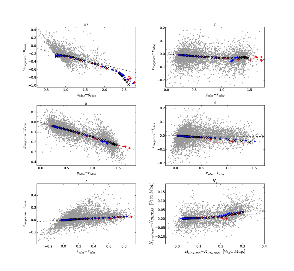
Because the transformations are an important element of the calibration of the magnitude zero points in this section, we display them in the first five panels of Figure 1 together with stars common to NGVS and SDSS. The amplitude of the dispersion is primarily due to the random photometric erros in SDSS. Only one zero point per image is derived in the calibration against SDSS, hence the relevant errors are the average differences between the various displayed loci (over the range of colors most populated with stars). The NGVS magnitudes used in the figure are taken after calibration, hence by construction the stars are located, on average, on the calibration line, with (sample dependent) mean offsets smaller than 0.01 mag.
The transformations are also compared with those obtained from synthetic photometry in Figure 1. We used three libraries of synthetic stellar spectra: the MARCS library of Gustafsson et al. (2008), the BaSeL 3.1 library (Lejeune et al. 1997, Lejeune et al. 1998 and Westera et al. 2002) and the PHOENIX library of Husser et al. (2013). The assumed stellar temperatures, surface gravities and metallicities along the NGVS stellar locus are obtained from the Besançon model of the Milky Way (Robin et al. 2003, Robin et al. 2004), to which adequate magnitude cuts were applied. For reasons that will become apparent in Section 2.6, our preferred library is the PHOENIX library.
The transmission curves for the synthetic photometry were taken from Betoule et al. (2013) for MegaCam444Betoule et al. provide transmissions for various annuli around the center of the MegaCam field of view. We use the fourth radius (70 mm from the center of the filter), which within a few millimagnitudes is equivalent to using an area-weighted average of the local transmissions.. It includes all telescope and instrument components as well as typical telluric absorption features555The transmission curves are available with the online version of this paper..
Although the transformation equations are not actually fits to the synthetic data, the similarity is quite impressive. Average residuals between the synthetic data and the reference lines (over the range of colors most populated with NGVS+SDSS stars and hence most relevant to the calibration) are smaller than 0.01 mag, i.e. smaller than the dispersion expected from the photometric errors of SDSS. We note that there are essentially no stars of type F and hotter in the calibration sample. Had there been many, a linear transformation equation would have been inadequate for . Indeed, rapidly deviates from a straight line when , as a consequence of the strong Balmer jump in the spectra of hotter stars.
In the near-infrared, we tied the WIRCam photometry to UKIDSS DR8 (Hewett et al. 2006, Dye et al. 2006, Hodgkin et al. 2009)666The aperture-corrected magnitudes provided in UKIDSS catalogs as kAperMag3 are used for stars. Although shallower by about 3 magnitudes than NGVS-IR, the UKIDSS point source catalog is deeper and more precise than 2MASS.
Both UKIDSS and 2MASS band transmissions have larger effective wavelengths than the WIRCam filter (for which an all inclusive transmission curve is given in Muñoz et al. 2014). Over the range of colors of stars in common with NGVS-IR, i.e. mag, the quantity varies with a global dependence on color given by (Muñoz et al., 2014). Note that in this expression is the native UKIDSS value, in Vega magnitudes, while we use AB magnitudes everywhere else in this paper ( [AB] = [Vega] + 1.827, Muñoz et al. 2014). The actual relation between and color is not linear but shows curvature over the whole color range, and starts off essentially flat for 0.2 mag (last panel of Fig. 1). We have used the synthetic values of in this restricted range of colors for the re-calibration of the NGVS-IR zero point, because all the collections of stellar spectra agree there, while cool M dwarf models become progressively more uncertain at lower temperatures.
The NGVS photometry obtained here is used as a default in the remainder of this paper. A budget of systematic errors is given in the context of globular cluster photometry in Section 3.6 (subsections 3.6.1 to 3.6.3, and Tab. 5). An alternative calibration based on the direct comparison of empirical and synthetic stellar loci in color-color planes is considered in Section 2.6, but then only used as a second choice in the Appendix.
2.5. Extinction correction
The foreground extinction towards the Virgo core region is low. Schlegel et al. (1998) report 0.06 A(V) 0.16, while Schlafly & Finkbeiner (2011) produce values that are typically 15 % lower. Over 90 % of the field, including the M87 region, A(V) 0.10.
Extinction coefficients for the MegaCam and WIRCam filters were provided in an appendix of Muñoz et al. (2014), using the extinction law of Cardelli et al. (1989) with R(V) = 3.1 and stellar spectra of a variety of spectral types. We have used the values they derived for a solar type star. Changes between extreme stellar types lead to changes in smaller than 0.02 in , , and , than 0.03 in and than 0.07 . Towards Virgo, errors on due to the color-dependence of extinction coefficients are therefore smaller than 0.01 mag.
Based on the above, typical reddening corrections amount 0.06 mag in , and 0.04 mag in and . Rescaling A(V) from the value of Schlegel et al. (1998) to that of Schlafly & Finkbeiner (2011) reduces towards M87 by 0.011 mag and by 0.007 mag. In the following, when correcting for extinction on individual lines of sight, we have used the values of E(B-V) of Schlegel et al. (1998) for consistency with previous publications of the NGVS collaboration.
2.6. Alternative calibration via Stellar Locus Regression
As mentioned earlier, we have explored a second calibration method, that relies on synthetic colors of stars instead of the stellar fluxes of external surveys. Although this new method looks promising, the choice of an external spectral library as a reference remains a limiting factor. Hence, we restrict this section to a description of the method and its key ingredients, and to an assessment of the differences with the the previous photometry. We then use the calibration in Section 2.4 for the analysis of GCs. Further details relevant to the alternative calibration method, and a repetition of some of the GC analysis with that calibration, are made available in the Appendix.
2.6.1 The SLR Method
Stellar Locus Regression (SLR) was introduced under this name by High et al. (2009), who used it to calibrate colors of new photometric surveys against colors in pre-existing, supposedly well-calibrated ones. In brief, the method forces the loci of point sources in color-color space to agree in the two surveys, assuming this locus is (at least roughly) universal. It does not provide an absolute flux calibration, but explicitely focuses on colors. Here, we have adapted the method to attach the NGVS/NGVS-IR stellar locus to the locus predicted by theoretical stellar spectra.
In principle, it makes sense to require a good match between empirical and synthetic stellar colors whenever the final purpose is to compare empirical colors of stellar populations with synthetic ones. However, in practice this test is not as relevant as it may seem: the stars we see in surveys such as the NGVS are essentially all on the lower main sequence, while the red and near-IR light of globular clusters or galaxies comes mostly from red giants. Here, we explore this second calibration simply as an alternative to the calibration against SDSS and UKIDSS. As a side product, this allows us to assess model spectra of cool dwarf stars.
In the SLR of High et al. (2009), the color transformation equation is written as
| (1) |
where is a vector of new (possibly uncalibrated) colors, is the vector of assumed true colors (the reference color locus), accounts for zero point shifts due for instance to atmospheric extinction and differences between the effective wavelengths of the used and reference filters, and is the color transformation matrix. The method assumes that the color transformations between the reference and adopted passbands are known, i.e. is known (from standard star observations). The problem is then essentially reduced to searching for the optimal offsets .
In our case, we use synthetic photometry as a reference and we assume the NGVS and NGVS-IR transmission curves are well known, so Eq. 1 reduces to .
The stellar locus regression has been implemented as in High et al. (2009): we minimize the weighted sum of the color-distances between the dereddened empirical stellar colors, after shifting with , and the respectively closest point on the synthetic locus. The photometric errors are used for the inverse-variance weighting.
2.6.2 Choice of a reference library and of fitted colors
The main difficulty in the application of the SLR is the choice of the reference stellar locus. The results also depend on the choice of colors used in the fit.
High et al. (2009) advise against using SLR for the filter due to the large dependence of band fluxes on stellar metallicity and galactic dust extinction. Thus, we have decided to determine SLR shifts only for , , , and at first, which sample the energy distribution from to . The effects of including the band in the SLR calibration procedure are briefly assessed in the Appendix (Fig. 22 and corresponding text). We confirm that the near-ultraviolet raises stronger issues than other bands.
The first three of the colors listed above are the ones also used by High et al. (2009). As these authors highlight, the colors must be chosen so the stellar locus displays a kink in at least one color-color plane, otherwise the fit is not well constrained (the offsets along the stellar locus would be arbitrary). Our choice satisfies this requirement as subsequent figures will show.
As a source of stellar spectra for synthetic photometry, we have used the collections already mentioned in Section 2.4: the PHOENIX theoretical spectral library of Husser et al. (2013), the MARCS model collection of Gustafsson et al. (2008), and the semi-empirical library BaSeL 3.1. We also considered the empirical library of Pickles (1998), which has robust colors for near-solar metallicity, but we ended up not using it because its sampling of metallicity is too scarce. While all these libraries agree rather well for the colors of main sequence stars of types F to K, their colors fan out in very different ways at cool temperatures, where the molecular bands of M dwarfs become increasingly important.
The typical stellar properties of the NGVS stars vary along the stellar locus from Milky Way halo-like at the blue end, to thin and thick disk-like at the red end. The stellar parameters we used are derived from the Besançon model of the Milky Way (Robin et al., 2003, 2004)777Version available on line in early 2015. in the NGVS footprint, taking into account the saturation and detection limits of the survey in all passbands. Besançon model stars were sorted into bins of 500 K width, from 3000 K to 6500 K. The statistical properties of log(g), [Fe/H], [/Fe] that we have used to choose spectra for each bin are listed in Table 1. We note that the BaSeL library has only solar abundance ratios, so in that case changes of [/Fe] were not accounted for.
| Teff (K) | log(g) | [Fe/H] | [/Fe] |
|---|---|---|---|
| 3100 | 5 | 0.0 | 0.0 |
| 3600 | 5 | -0.5 | 0.2 |
| 4000 | 5 | -1 | 0.2 |
| 4500 | 5 | -1.5 | 0.4 |
| 5000 | 4.5 | -1.5 | 0.4 |
| 5500 | 4.5 | -1.5 | 0.4 |
| 6000 | 4.5 | -1.5 | 0.4 |
| 6400 | 4.5 | -2 | 0.4 |
In Figure 2, the BaSeL (red), PHOENIX (black) and MARCS (blue) libraries are shown superimposed to our NGVS stellar locus. At the red end, the discrepancies between those libraries are large. The PHOENIX library fits the shape of our empirical distributions well in all color-color diagrams, with only a small tilt of the M-dwarf sequence with respect to observations in the plot of vs. . As only shifts and not change of shape are allowed in the SLR calibration, we conclude that only the PHOENIX library is appropriate for our purpose, and we discard other libraries in the remainder of this section.
Important features in these color-color diagrams are the kinks seen in all but the diagrams. The locus of these kinks controls shifts along the color-color sequences of stars. As these shifts are also applied to globular clusters, they directly affect the metallicity estimates of the latter.
2.6.3 SLR results
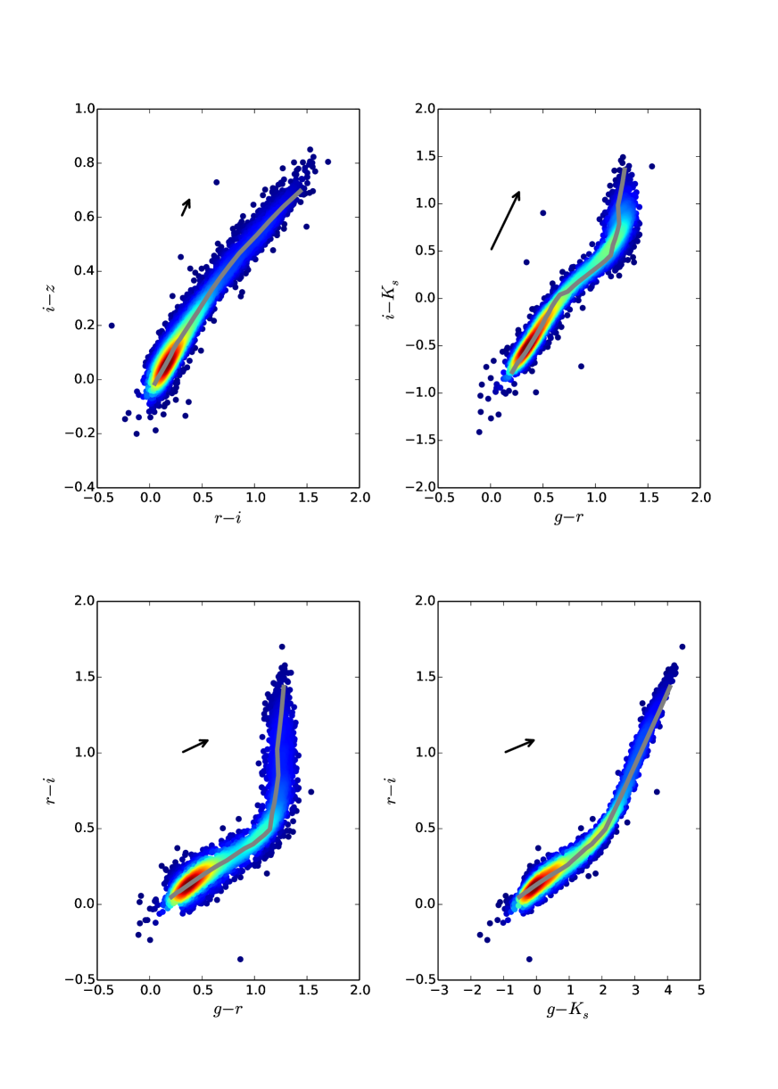
To account for spatial variations of extinction over the area of the survey, we deredden NGVS stars before estimating the best vector of corrections, . We then apply these corrections to all objects in the NGVS data set. Figure 3 shows the stellar locus obtained after the SLR calibration and the arrow illustrates the displacement applied.
The SLR offsets found with the method above are
.
The offsets in and are marginally consistent with our estimated bounds on errors in Section 3.6.
The shifts in and are larger than expected.
Figure 3 shows this may be related to the slight tilt of the slope of the PHOENIX sequence in the and planes.
The slope on the red side of the kink in the stellar locus differs between models and the observations. partly
compensates for the difference this generates at low temperatures.
2.6.4 Summary of the photometric calibration
Our default photometric calibration rests on three steps: the construction of image stacks that account for differences in photometric zero points between detector chips, the computation of local aperture corrections for point sources, and the comparison with SDSS and UKIDSS (after transformation to the NGVS passbands). We use the extinction map of Schlegel et al. (1998) but have provided the comparison with Schlafly & Finkbeiner (2011) in Section 2.5.
We have also implemented an alternative calibration of the colors, based on stellar spectral libraries, a model for the stellar population of the Milky Way, and synthetic photometry. Because some of the color shifts suggested by that calibration are large, we suspect biases exist even in the best models for the colors of lower main sequence stars on the line of sight towards Virgo. Our preferred calibration to date is the first one.
3. The globular cluster sample
3.1. Selection
The selection of the globular clusters is a crucial point in our study. Our purpose is to provide typical globular cluster colors and SEDs as a benchmark for comparisons with model predictions, not to discuss the number distribution of globular clusters over the range of possible colors.Therefore, our main concern is to limit contamination by foreground stars or background galaxies and to work with objects that have good photometry. Completeness is not a target, except that we wish to sample the whole range of colors along the main direction of the GC color sequence.
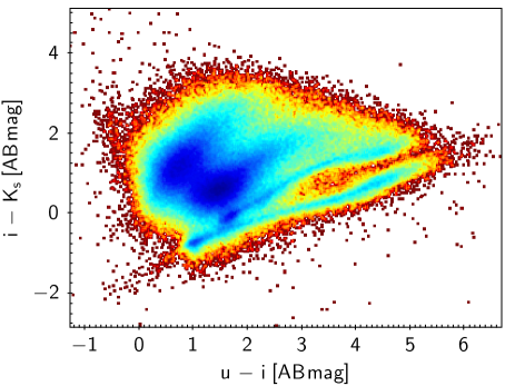
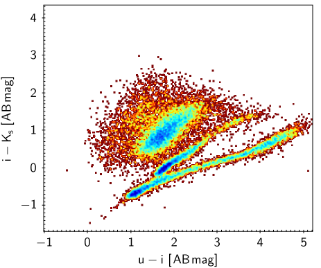
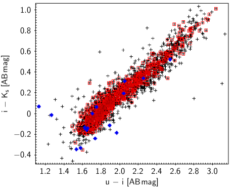
Our starting point is a merged NGVS + NGVS-IR catalog of over a million sources in the Virgo core region. Preliminary processing includes the rejection of objects that lack data in one or more filters (catalog magnitude 60), the rejection of sources with magnitude error larger than 0.5 mag, and the removal of duplicate or erroneous objects in regions of overlap between pointings. Figure 4 shows this catalog in the diagram (Muñoz et al., 2014). From red to blue colors, the most conspicuous sequences in this diagram correspond to background galaxies with various star forming histories at redshifts up to , globular clusters (which merge into the redshift sequence of passive galaxies at the red end), and foreground main sequence stars. Although the diagram provides a better separation between sequences than any other color-color diagram, there is a significant overlap between populations in this deep and exhaustive catalog.
At this point, we applied stricter selection criteria on our sample to remove saturated sources (the limit depends on the filter and on the seeing but it is typically around 18 mag [AB] whatever the filter), large objects (half-flux radius 4 pixels) and sources with large errors (SExtractor errors 0.06 mag in any filter). The sources surviving these cuts are shown in the top panel of Figure 5.
Our final cleaned selection then exploits both the diagram and size information. Massive globular clusters and DGTOs (Dwarf Galaxy Transition Objects) in Virgo are marginally resolved in images with 0.6″ seeing (48 pc), such as the NGVS and NGVS-IR images. Absolute sizes vary accross the pilot region because the various individual fields were observed in different seeing conditions. A good way to quantify whether an object is more spatially extended than a star is to compute the difference between two aperture-corrected magnitudes in the same filter. We will write such differences APCORn-APCORm, with n and m standing for the aperture diameters in pixels. These differences are on average zero for stars (the local aperture correction absorbs any spatial variations of the PSF), but are positive for extended sources. We have used both APCOR4-APCOR8 and APCOR4-APCOR16, finding that both behave similarly. In the standard diagram [ on the y-axis, on the x-axis], extended objects tend to lie to the upper left of the stellar sequence. By adding (APCOR4-APCOR8)(i) to and subtracting that quantity from , extended sources are efficiently moved away from the stellar sequence. Moreover, this translation effect can be improved by adding a non-linear function of (APCOR4-APCOR8)(). Our implementation depends more strongly on compactness outside the supposed range of GC colors as indicated in Eq. 2 and Eq. 3. This may bias slightly against possible unresolved blue clusters, but improves the rejection of stellar contaminants.
Between and :
| (2) |
Outside this range:
| (3) |
where the constant is set by the requirement of continuity at and . In our case, and .
This ‘modified’ diagram is shown in the bottom panel of Figure 5.
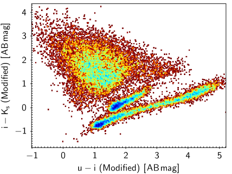
In the standard diagram, the GC sequence suffers from contamination by halo main sequence stars, in particular at the blue end. It is fortunate that blue clusters tend to be the most extended (Jordán et al., 2005): taking size into account therefore effectively separates halo stars from blue globular clusters. At the red end, many extended passive galaxies are also efficiently moved away from the globular cluster sequence.
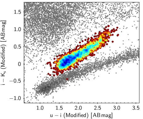
The final selection of GCs, shown in Figure 6, is obtained by applying a conservative sigma clipping algorithm in the modified diagram. We use a polynomial fit of the current GC locus as a reference and broaden it by 0.1 mag in both colors. GCs distant from this broad locus by more than 3 times the uncertainty on their colors are rejected. We are left with 2321 globular clusters with median errors in of, respectively, 0.02, 0.008, 0.008, 0.01, 0.02 and 0.08 mag. In the following subsection, we compare our selected globular clusters to several spectroscopic datasets from the literature.
3.2. Comparison with spectroscopic samples
The NGVS collaboration maintains a ‘master spectroscopic catalogue’ that includes all objects within the NGVS footprint with measured redshifts, collected from the literature, or part of the NGVS collaboration efforts to target objects in the field. In particular, data from the literature includes the SDSS DR10 release, the NASA Extragalactic Database for extended objects (Binggeli et al., 1985), and catalogues of Hanes et al. (2001), and Strader et al. (2011). Spectroscopic campaign were carried out by the NGVS team using Anglo-Australian Telescope 2dF observations and Multiple Mirror Telescope Hectospec observations by E. Peng and Keck DEIMOS observations by R. Guhathakurta.
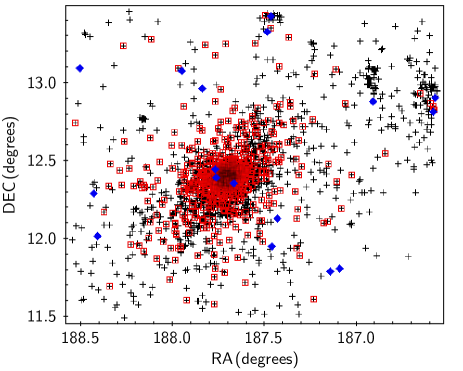
Among our selection of 2321 globular clusters, 783 have a measured redshift. All but 17 are bona fide Virgo globular clusters according to the spectroscopic data. Among those 17, 5 are considered galaxies and 12 stars. Figure 7 shows our sample together with the matched spectroscopic targets in RA-DEC (left) and in color-color space (right). Globular cluster overdensities are visible near M87 but also around NGC 4473, NGC 4438 or M86 (in the North-West corner of the field, from the East to the West). We note that the spectroscopic catalog has no objects associated with NGC 4438 and NGC 4435.
Extrapolating from this test, we estimate the contamination of our full GC sample to be limited to about 50 objects out of 2321 (i.e. about 2 %). Eyeball estimates based on the distribution of sources in the modified diagram (Fig. 5) would allow contaminations of up to 100 objects, i.e. about 5 %.
We note that the colors of the matched spectroscopic sample span the whole range of colors of our photometric GC catalog (Fig. 7). This provides confidence that our reddest objects are not background ellipticals and our bluest ones not foreground stars.
3.3. Aperture photometry of globular clusters
As globular clusters are marginally resolved sources in the NGVS survey, the point source aperture corrections do not strictly apply to them. However, these aperture corrections efficiently absorb the spatial variations of the PSF (mostly due to seeing variations with time), and we can limit any bias in color measurements by applying aperture corrections to relatively large measurement apertures.
To test this assertion, we have compared aperture-corrected magnitudes (APCOR-magnitudes hereafter) and the corresponding colors (APCOR-colors) as a function of the compactness parameter already used earlier (APCOR4-APCOR8 in the band). As expected, the comparison between globular cluster APCOR-colors measured in 2 apertures of which one is small, shows a difference that depends strongly on compactness. For example for apertures of 4 and 8 pixels the amplitude of this trend along the GC compactness-sequence exceeds 0.1 mag for , and . However, the amplitude of the trend drops to 0.01 mag or less in all colors when APCOR-colors in 7 and 8 pixels are compared (we note that the difference between APCOR-magnitudes from 7 and 8 pixels still changes by 0.03 mag along the compactness-sequence). For apertures larger than 8 pixels, for instance APCOR-colors measured in 8 and 16 pixels, no systematic trends with compactness are detected. The discussion in this paper is based on APCOR-colors measured in 8 pixel apertures, APCOR16 colors being noisier for faint objects.
3.4. r band seeing issues
During the data acquisition for NGVS pointing +0+0 in the band (the pointing containing M87), the seeing has varied significantly more than for all other pointings and filters. As a consequence, the point sources located along the gaps between the individual rows of detectors have sizes that differ from other locations (the number of exposures combined in these pixels is smaller than elsewhere). The local aperture corrections cannot be determined with a spatial sampling as small as these gaps. The consequences are outliers in color-color diagrams that involve the band. Figure 8 shows the effect on the globular cluster sequence: two abnormal branches are seen on either side of the main locus.
Our goal is to have a clean sample of GC colors. Thus for the purpose of this paper we have removed all the objects with abnormal -band photometry from our reference sample. This last modification reduced our sample from 2321 to 1846 globular clusters.
3.5. Properties of the GC sample
At this point, we have a clean sample of 1846 globular clusters. As announced previously, this catalog is available in numerical form and an extract is given in Tab. 2.
| RA | 187.546 | Right ascension |
| DEC | 13.166 | Declination |
| E(B-V) | 0.023 | Exctinction |
| u*mag_ap8 | 23.713 | |
| gmag_ap8 | 22.236 | |
| rmag_ap8 | 21.332 | aperture corrected magnitude |
| imag_ap8 | 20.900 | based on 8 pixel aperture |
| zmag_ap8 | 20.634 | |
| Ksmag_ap8 | 20.105 | |
| u*mag_ap8_0 | 23.608 | |
| gmag_ap8_0 | 22.154 | |
| rmag_ap8_0 | 21.271 | aperture corrected magnitude, |
| imag_ap8_0 | 20.853 | dereddened |
| zmag_ap8_0 | 20.599 | |
| Ksmag_ap8_0 | 20.096 | |
| u*err_ap8 | 0.039 | |
| gerr_ap8 | 0.011 | |
| rerr_ap8 | 0.008 | 1 error on magnitude |
| ierr_ap8 | 0.011 | in 8 pixel aperture |
| zerr_ap8 | 0.016 | |
| Kserr_ap8 | 0.051 | |
| (u*-g)_cal | 1.454 | |
| (g-r)_cal | 0.883 | |
| (r-i)_cal | 0.418 | color, dereddened |
| (i-z)_cal | 0.254 | |
| (i-Ks)_cal | 0.757 | |
| (g-r)_cal.slr | 0.941 | |
| (r-i)_cal.slr | 0.437 | color, dereddened, |
| (i-z)_cal.slr | 0.270 | after re-calibration with SLR |
| (i-Ks)_cal.slr | 0.890 |
This GC sample is designed to provide a robust reference locus in color space, as opposed to being complete in volume or magnitude. Each of the 1846 clusters was selected to have good photometry across the whole spectrum. The population of the red end of the GC sequence (metal rich clusters) is limited by the requirement of good quality photometry, and the number of objects at the blue end by requirements in and . The typical magnitudes of the GCs in the sample are provided in Tab. 3. At the blue end of the sequence, this corresponds to typical masses of , and at the red end to masses of . These masses are typically a factor of 10 above the turn-over of the GC mass function (Jordán et al., 2007).
| Mean | 10 % | 90 % | Mean errors | |
|---|---|---|---|---|
| (1) | (2) | (3) | (4) | |
| 23.05 | 22.14 | 23.95 | 30 | |
| 21.88 | 21.00 | 22.63 | 9 | |
| 21.32 | 20.46 | 22.06 | 8 | |
| 21.05 | 20.20 | 21.77 | 12 | |
| 20.87 | 20.02 | 21.58 | 21 | |
| 20.90 | 20.02 | 21.66 | 83 |
Columns (2) and (3) provide the 10 % and 90 % percentiles of the distributions. The mean photometric errors are given in mmag.
Color distributions of the GCs will be discussed in detail in Section 5. Using these, we have determined fiducial loci in color-color diagrams, and fiducial SEDs for various locations along the GC sequence. The purpose of these is to provide an easy graphical reference when comparing color distributions with models (Section 5). As the Virgo core region contains GCs with a variety of histories and environements, one may expect different GCs to contain different stellar populations (age, metallicity, chemical abundances, etc), and we warn that the fiducial SEDs would not capture this diversity.
The fiducial SEDs are based on maximum likelihood polynomial fits to GC color-color distributions. The likelihood of a polynomial is the probability of obtaining the observed color-color distribution when drawing from this polynomial parent distribution, taking into account the errors on the colors and their covariance (we treat the errors as gaussian in this process). Numerically, the polynomial is segmented into a large number of small segments , which are here assigned equal prior probability (flat prior).
Here is the probability, for cluster in the sample, to be observed with colors if it originally was located on the polynomial, and is the same for location on the polynomial. is a constant.
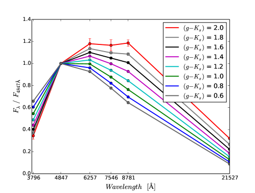
Figure 9 shows a set of fiducial SEDs obtained as a function of , a color with a large range of values compared to error bars. To first order, the sequence may be seen as an empirical illustration of the effects of metallicity, combined with a possible effect of age. To define these SEDs, polynomials were fitted respectively to the loci in diagrams of , , , and versus . The values of the polynomials at a set of colors define the fiducial SEDs.
Thanks to the large number of clusters and to the small individual photometric errors for each GC, the fiducial sequence is extremely well defined. Bootstrap resampling provides the 3 error bars shown in Fig. 9 (most of these are too small to see, and all are smaller than the systematic errors on the GC photometry). The fiducial SEDs can also be modified by changing the order of the adopted polynomial, removing more or fewer outliers, and other fitting process differences. However the modifications obtained with various reasonable variants of the fitting details are of small amplitude compared to the systematic effects we intend to discuss in the comparison with models later on.
To conclude the description of the sample, we have tested whether or not the empirical GC color distribution is statistically compatible with an infinitely tight theoretical color-locus, given by the fiducial SEDs just described. To quantify the goodness-of-fit, we used the following reduced :
| (4) |
where contains the colors considered, is the covariance matrix, holds the colors of a point of the fiducial locus, and takes the minimum along the polynomial. is a proxy for the number of degrees of freedom of the fit.
We fitted two-color distributions with polynomials of orders 2 to 5, and explored the effects of removing up ten GCs with strongest individual impacts on the fit and the . All in all, using several combinaisons of colors, we did not find a best below 1.23 for a single color-color diagram. Conversely, we found a number of color-color planes in which the best in these tests remained above 3, for instance vs. , or vs . For good representations of the data, the would not exceed 1 by more than a few (i.e. a few times 0.023). Hence there is real dispersion across the main locus of the data.
| Fu*/Fg | Fg/Fg | Fr/Fg | Fi/Fg | Fz/Fg | FKs/Fg | |||||
|---|---|---|---|---|---|---|---|---|---|---|
| =0.4 | 0.697 | 1.000 | 0.896 | 0.741 | 0.606 | 0.073 | 0.923 | 0.435 | 0.636 | 0.747 |
| =0.6 | 0.658 | 1.000 | 0.928 | 0.777 | 0.645 | 0.088 | 0.985 | 0.472 | 0.687 | 0.814 |
| =0.8 | 0.604 | 1.000 | 0.960 | 0.821 | 0.696 | 0.106 | 1.078 | 0.511 | 0.747 | 0.897 |
| =1.0 | 0.545 | 1.000 | 0.996 | 0.877 | 0.764 | 0.127 | 1.190 | 0.550 | 0.818 | 0.998 |
| =1.2 | 0.489 | 1.000 | 1.032 | 0.938 | 0.844 | 0.153 | 1.309 | 0.589 | 0.892 | 1.106 |
| =1.4 | 0.441 | 1.000 | 1.067 | 0.998 | 0.928 | 0.184 | 1.421 | 0.625 | 0.959 | 1.209 |
| =1.6 | 0.402 | 1.000 | 1.100 | 1.049 | 1.008 | 0.221 | 1.520 | 0.658 | 1.013 | 1.299 |
| =1.8 | 0.372 | 1.000 | 1.135 | 1.097 | 1.085 | 0.266 | 1.605 | 0.692 | 1.062 | 1.379 |
| =2.0 | 0.344 | 1.000 | 1.179 | 1.165 | 1.186 | 0.320 | 1.691 | 0.734 | 1.127 | 1.475 |
Notes: The flux ratios are taken in arbitrary units of energy per unit wavelength interval, and the color indices are in AB magnitudes.
3.6. Budget of systematic errors
The online catalog of GCs provides individual uncertainties on the magnitude measurements, as described in Section 2.4. In addition to these random errors, we have mentioned a variety of sources of possible systematic errors on the photometry. We provide a summary of these here, with estimated bounds in Tab. 5.
3.6.1 Systematic errors in the external reference catalogs
The NGVS MegaCam photometry is calibrated against SDSS stars, thus any
systematic errors in the SDSS photometry has a direct effect on NGVS.
Currently, the relative calibration within SDSS DR10 seems to be well
known, with studies by Padmanabhan et al. (2008), Bramich & Freudling (2012), Schlafly & Finkbeiner (2011). The precision of the internal
calibration is estimated to be around 2 % in the band and 1 % in the
, , and filters. Regarding the absolute calibration of SDSS (which
is known not to be on an exact AB magnitude system), limits are more
difficult to set. The SDSS DR10
documentation888https://www.sdss3.org/dr10/algorithms/fluxcal.php indicates
a likely offset of 0.04 mag in , in the sense that . An offset of 0.02 mag in in the opposite direction is
also advocated there. These offsets are considered known to no better
than 0.01 mag, and possibly slightly less precisely for .
We have not implemented these zero point shifts in our
data but discuss their effect whenever
necessary. In summary,
we adopt limits on the systematic errors of 0.04 mag
in the filter, 0.01 mag in , , , and 0.02 mag in , and note that there is a preferred direction
for the offsets in and 999More specifically, users who wish to
apply the conversions from SDSS to AB magnitudes suggested by the SDSS
web pages should remove 0.04 mag from the NGVS values
published in this paper and add 0.02
mag to the NGVS values. After these corrections, one may consider
reducing the SDSS calibration errors to 0.015 in and 0.01 in .
Similarly, the band is affected by any systematic errors in the
UKIDSS photometry (DR8). Based on the various tests presented by Hodgkin et al. (2009), we assign a bound of 0.02 magnitudes on systematic errors
to this photometry.
3.6.2 Systematic errors in the calibration of NGVS with respect to the external catalogs
The calibration of NGVS relative to SDSS or UKIDSS is affected slightly by the dispersion in the photometry of stars in common between the surveys. The dispersion seen around the mean trend in the calibration figures (Fig. 1) is due mainly to dispersion in the SDSS and 2MASS/UKIDSS catalogs, NGVS being deeper. The number of stars available for the calibration reduces errors on the mean to a few millimagnitudes in all filters.
Small differences are seen in Fig. 1 between the reference transformation curve used in the , , , , data processing and modern synthetic photometry. We take this as an indication of possible systematics in the transformation between systems. As an estimate of their amplitude, we adopt the mean difference between the empirical and the synthetic loci, over the range of colors of stars actually observed in the survey. The offsets are smaller than 50 mmag in , 5 mmag in , 5 mmag in , 8 mmag in , and 2 mmag in .
The transmission curves adopted for NGVS have impact on the locus of synthetic colors in the calibration figures (Fig. 1). A few versions of the Megacam filters have been available on CFHT/CADC web pages over the years, prior to the work of Betoule et al. (2013). Our test for two extreme sets of filters results in discrepancies inferior to 12 mmag in , 2 mmag in ,, 3 mmag in and 8 mmag in . If we estimate the main source of uncertainty in the WIRCam transmission is telluric absorption, we find that reasonable changes in airmass/humidity change the magnitudes by less than 5 mmag.
Our calibration of the WIRCam photometry against UKIDSS involves a conversion from AB magnitudes to Vega magnitudes. We have converted our WIRCam AB magnitudes to Vega magnitudes for this purpose. The offset used, determined in Muñoz et al. (2014), is based to the best of our knowledge, on the same reference Vega spectrum as used for UKIDSS (Hewett et al., 2006), i.e. a spectrum originally provided by Bohlin & Gilliland (2004)101010That Vega spectrum was made available at the time on the Hubble Space Telescope Science Institute web pages as alpha.lyr.stis.003 or alpha.lyr.stis.005, these two files leading to identical results for the band.. Therefore we take it that this source of error adds little to those already included in the absolute UKIDSS errors and the errors due to transmission changes, described above.
3.6.3 Systematic errors in the reddening corrections
Systematic errors can also occur in the dereddening process, with the choice of a particular local value of A(V) or E(B-V), and of wavelength dependent extinction coefficients. The different total extinction estimates of Schlegel et al. (1998) and Schlafly & Finkbeiner (2011) translate into differences of 19 mmag for , 14 mmag for , 11 mmag for , 8 mmag for , 6 mmag for and 1 mmag for when using the extinction law of Cardelli et al. (1989), in the sense that the Schlafly & Finkbeiner (2011) reddening corrections are smaller (cf. Section 2.5). The use of extreme stellar types to derive extinction coefficients for a given extinction law produces a span of extinction magnitudes in the Virgo region inferior to 5 mmag in , 10 mmag in , and 2 mmag for the , , and filters. Using the extinction law of Fitzpatrick (1999) instead of Cardelli et al. (1989) changes Virgo magnitudes by 10 mmag maximum.
| Maximum estimated errors in mmag. | ||||||
|---|---|---|---|---|---|---|
| SDSS calibration | 40 | 10 | 10 | 10 | 20 | |
| UKIDSS calibration | 20 | |||||
| Transformation between systems | 50 | 5 | 5 | 8 | 2 | |
| Color dependance of extinction coefficients | 5 | 10 | 2 | 2 | 2 | 2 |
| A(V): Schlafly vs Schlegel | 19 | 14 | 11 | 8 | 6 | 1 |
| Filter transmissions | 12 | 2 | 3 | 2 | 8 | 5 |
Note that uncertainties on A(V) creates systematics that are not independent between passbands. See Section 3.6.1 for the preferred direction of the systematic errors on the SDSS calibration in and .
3.6.4 Systematic errors in the SLR method
The SLR method relies on spectral libraries and transmission curves. The use of a different library or a different set of stellar parameters along the stellar locus can induce very large changes of the vector of color-shifts, . For example, the differences between our preferred set of parameters (black line in Fig. 3) and a set composed of solar metallicity stars all with [/Fe] = 0 and log(g) = 5.0 produces a color difference of (mmag.) = [() = 37, () = 19,() = 15, () = 2]. The varying parameters given by the Besançon model of the Milky Way are more reasonable than a set with uniform composition and gravity, reducing this source of systematics somewhat.
Having described our empirical GC sample and its photometric accuracy, we turn towards population synthesis models and predicted colors. The comparison between models and data in color-color diagrams (Section 5) serves to characterize the empirical color locus further, and is a fundamental step towards estimating the evolutionary parameters of the clusters.
4. The models
Numerous population synthesis models are available in the literature and can be used to estimate ages and metallicities of stellar populations from empirical SEDs. In this section, we describe the codes we have used, as well as the generic assumptions made to construct synthetic SEDs for globular clusters with each of them. Comparisons between the resulting SEDs, and with the NGVS globular cluster colors, are made in Section 5.
In this paper, we consider only models for single stellar populations, containing stars of a single age and chemical composition. This assumption is questionable, especially for a sample of massive clusters, since photometric and spectroscopic studies of resolved massive clusters nearby revealed the existence of multiple subpopulations. Our analysis is meant to provide a reference point for future studies, in which these assumptions could be relaxed.
We have considered six commonly used stellar population synthesis codes (SPS codes hereafter), for which predictions can be obtained via dedicated webpages.
From each SPS code, we obtained a set of synthetic spectral energy distributions for single stellar populations, i.e. synthetic SSP models (sSSP hereafter). [Fe/H] was varied from -2 to 0.17 (with three exceptions among the 11 sSSPs mentioned below), and ages between 6 and 13 Gyr. The majority of the GCs in the Virgo sample are assumed to be old. Nevertheless, these restrictions on age and metallicity must be kept in mind in the comparisons below, and possibly be relaxed in future studies of individual objects.
We adopted the initial mass function (IMF) of Kroupa (1998) or Kroupa (2001) as available with the codes. The discrepancies due to changes in the IMF are smaller than other discrepancies between model families, so we will not show any assessments of these here.
Whenever possible, we used the SPS codes to compute synthetic spectra, and derived synthetic photometry from them ourselves with the filters described in Section 2.4. For codes that allow the input of customized transmission curves, we compared our synthetic photometry with the one produced by those codes, finding that differences were negligible (less than 0.05 %).
To account for the redshift effect, we have computed all the model colors at the typical redshift of the Virgo cluster. This correction (which reaches 15 mmag in the band and 5 mmag in the band) has been obtained directly by a computation of the colors on a redshifted spectrum, or otherwise by the use of a redshift-correction based on the Maraston (2005) model and the Pégase models.
The sSSP models differ from each other by the stellar evolution tracks they rest upon and by the stellar library used to predict spectrophotometric properties. We briefly describe these choices below.
Two first sets of sSSPs, labelled BC03 and BC03B hereafter, are taken from Bruzual & Charlot (2003)111111We use the 2012 update made available by the authors upon request, but it differs from the 2003 version only in additional outputs that we have not used.. We selected the 1994 version of the Padova isochrones as input (Alongi et al., 1993; Bressan et al., 1993; Fagotto et al., 1994a, b; Girardi et al., 1996). The default synthetic spectra (BC03) combine optical stellar spectra from STELIB (Le Borgne et al., 2003) between 3200 and 9500 Å with the BaSeL 3.1 spectral library outside this wavelength range (Lejeune et al. 1997, Lejeune et al. 1998 and Westera et al. 2002). For the BC03B set, the BaSeL stellar library was used instead at all wavelengths.
Three sets of sSSPs, labelled C09PB, C09BB and C09PM, are based on the Flexible Stellar Population Synthesis (v2.4) model of Conroy et al. (2009). The first one (C09PB) is computed with the Padova 2007 set of isochrones (Girardi et al., 2000; Marigo & Girardi, 2007; Marigo et al., 2008) and the BaSeL 3.1 spectral library. The second one (C09BB) is modeled with the BaSTI isochrones (Pietrinferni et al., 2004; Cordier et al., 2007) and the BaSeL 3.1 library. For the final one (C09PM), we used the Padova 2007 isochrones and the MILES spectral library (Sánchez-Blázquez et al., 2006). MILES spectra extend from 3500 to 7500 Å and can only provide fluxes in the and filters, so they are extended with the BaSeL spectral library beyond this range. The C09PM and C09BB sets do not reach down to [Fe/H] -2 dex, but instead respectively start at [Fe/H] = -1.39 and -1.82.
Two sets of sSSPs, labelled M05 and MS11, were constructed using the models of Maraston (2005) and Maraston & Strömbäck (2011). The former uses the Cassisi isochrones (Cassisi et al., 1997a, b, 2000) and the BaSeL 3.1 library. This model offers two options for the morphology of the horizontal branch (HB): a red HB and a bluer one. The red HB produced a better representation of our observations, so the blue HB will not be shown in this paper. The latter set (MS11) also uses the Cassisi isochrones and a combination of the MILES library and the BaSeL 3.1 library. Both these models are computed using algorithms based on fuel-consumption instead of the more common isochrone synthesis.
We also considered one model from the web interface CMD 2.7121212http://stev.oapd.inaf.it/cgi-bin/cmd provided by the Padova group (labelled PAD hereafter). This model uses the PARSEC 1.2S isochrones (Bressan et al., 2012; Tang et al., 2014; Chen et al., 2014, 2015) and it is based on the PHOENIX BT-Settl library (Allard et al., 2003) for effective temperatures lower than 4000 K, and on ATLAS9 ODFNEW (Castelli & Kurucz, 2004) otherwise. This version of PARSEC isochrones does not take into account thermally pulsing asymptotic giant branch (TP-AGB) stars. Although the tendency is for the estimated TP-AGB contributions to be revised downwards at old ages (Gullieuszik et al., 2008; Girardi et al., 2010; Melbourne et al., 2012; Rosenfield et al., 2014), the complete lack thereof is expected to produce a lack of near-infrared flux. Another issue with the PAD models is that no spectra are available from the web site. The synthetic photometry is based on filter transmissions older than the ones we now prefer. Discrepancies such as these may produce offsets of a few percent, in particular in .
The sSSP labelled PEG is produced with Pégase (Fioc & Rocca-Volmerange, 1997)131313We use the code made available as Pégase.2 or Pégase-HR by Le Borgne et al. (2004). The isochrones are the Padova 1994 set and the BaSeL 2.2 spectral library provides the photometry.
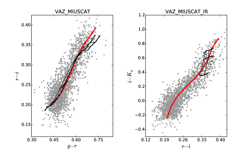
Finally, we have considered two sSSPs based on the model of Vazdekis et al. (2012). We have chosen to compute these models with the Padova 2000 isochrones. The first one, labelled VAZ_MIUSCAT, uses the MIUSCAT library with a wavelength range from 3464 to 9468 Å. It only allows us to compute the , and magnitudes. The second one, labelled VAZ_MIUSCAT_IR, is based on the MIUSCAT-IR library which extends from 3464 Å to 49999 Å. However, the values of [Fe/H] currently available for the spectra are restricted to -0.40, 0 or 0.22. Due to the wavelength and [Fe/H] ranges, the display of these sSSPs is done separately.
All these sSSPs are produced with the simplest assumptions possible: there is no dust (so no extinction), we chose default mass-loss parameters, zero binary fractions, etc. Overall, the aim was to compute for each SPS code the same distribution of GCs parameters.
5. Models versus data
To provide GC ages and metallicities, one needs to connect the various model predictions with the empirical GC color distributions. Because the age and metallicity information is hardwired in each model depending on the particular set of assumptions (see Section 4), we will pay particular attention to the differences in the derived GC age and metallicity distributions.
5.1. Optical-NIR color-color diagrams
Color-color diagrams provide a powerful global overview of all the assessed objects, as well as direct insight into the physical properties of GCs. In the case of old globular clusters, even a single color carries information on metallicity (e.g. Cantiello & Blakeslee 2007; Puzia et al. 2002), although as we shall emphasize the relation between color and [Fe/H] remains model-dependent. Color-color diagrams of GC samples in principle allow access to a second parameter, typically age. The distribution in the 5-dimensional color-space available for the NGVS clusters should improve the age and metallicity assessments. In practice however, they also highlight differences between models.
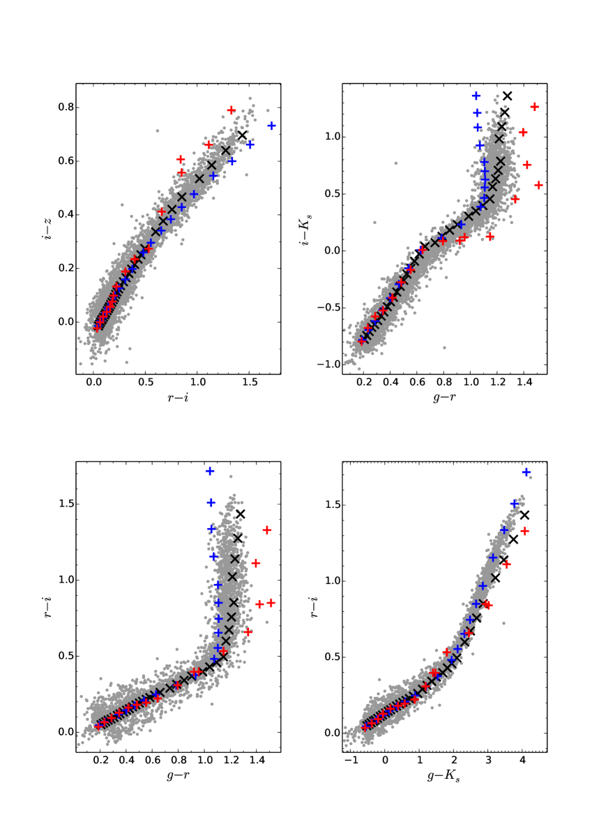
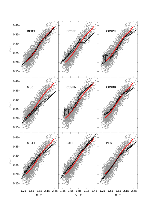
The locus of sSSP models with respect to the robust NGVS globular cluster sample in various color-color diagrams is shown in Figs. 10, 11, 12, and 13 (additional color-color diagrams are shown in Figure 24 of the Appendix). The first two are restricted to the MegaCam colors , , , and , the last two include .
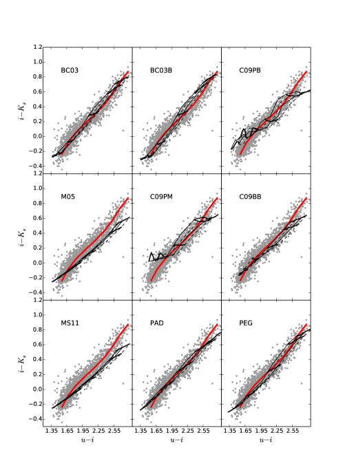
In the diagram ( vs. , Fig. 10), age and metallicity are degenerate in the models. This is essentially also the case in the diagram ( vs. , Fig. 11) and the diagram ( vs. , Fig. 12). The age-metallicity degeneracy is best broken in planes such as the diagram of Fig. 13 ( vs. an optical color, here ). This property has already been highlighted in the literature (e.g. Puzia et al. 2002).
Large discrepancies are seen between models in all color-color planes, despite the fact that all model grids cover the same range in age and [Fe/H] (with the exception of C09PM and C09BB, that lack the lowest metallicities). A model set that seems best in one color-color plane is not usually best in all the others.
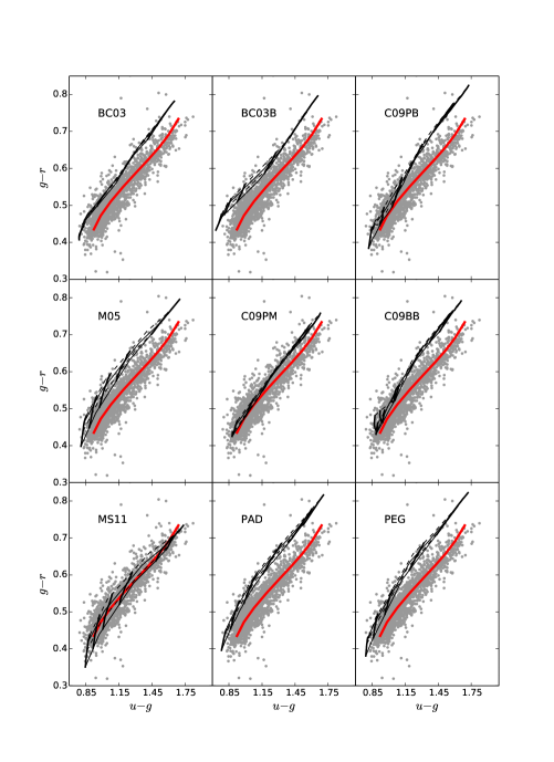
The range in color spanned by the models in and corresponds quite well to the range observed (Figs. 10 and 11). On the contrary, several models fall short of reproducing the observed range of colors in (Figs. 11 and 12), (Figs. 10 and 13) or . The models M05 and M11, which are known to have among the strongest AGB contributions in the literature at intermediate ages, struggle at older ages to reach the optical-near-IR colors of the reddest observed clusters. The PAD grid stops at an even smaller color index, about 0.1 mag bluer than the red end of the observed cluster distribution. This could seem a natural consequence of the lack of any TP-AGB stars in the PAD models, if this same model grid did not extend right to the end of the observed distributions in , or . In this case, this may argue for a systematic difference in the molecular absorption in the band between observed and synthetic GCs. The BC03 grid produces color ranges very similar to the PAD grid, although it is based on different isochrones and a different stellar library. BC03 and PAD however have in common that they do not use BaSeL, the library that provides and band fluxes in all other cases.
Now looking at the loci of the grids instead of their range in color, we find a variety of behaviors again. It is important to keep in mind that zero point offset errors in the NGVS photometry could shift the distributions but not modify their shape. Errors in individual extinction corrections would increase the dispersion. The shapes of the model grids could, on the other hand, be affected by errors in the assumed filter transmission curves as well as the input stellar physics.
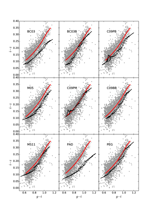
Surprisingly, it is in the diagram (Fig. 13) that the behaviour of the models is most uniformly satisfactory: the model grids are located within the bounds of the empirical color distribution, though sometimes with significant deviations from the fitted line of typical colors. As the color spreads of the various model grids differ, any given cluster could however be assigned rather different absolute metallicities and ages depending on the model adopted. In the diagram (Fig. 12), the model loci are satisfactory except for BC03 and PAD which, as already mentioned, do not produce red-enough colors at high metallicity. In the diagram (Fig. 11), the shapes of the model grids are mostly adequate, but a uniform offset in or in would seem required to match the data. Applying the offset of 0.02 mag in suggested by the SDSS DR10 calibration pages would act in the right direction for most models (see Section 3.6).
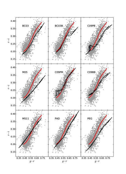
The purely optical diagram (Fig. 10) is not uniformly well matched. In several model grids, the slope of as a function of is too shallow compared to the data. In general, the models match the blue end of the GC distribution better than the red end. This could be because the Milky Way globular clusters frequently used to calibrate population synthesis models are mostly metal poor. However some models, such as C09PM or MS11, behave rather well at the red end in the plane. These two have in common that they exploit the MILES spectral library at optical wavelengths, which has an effect on the band fluxes (Maraston & Strömbäck 2011 and also Section 5.2). We confirmed this trend with the MIUSCAT/MILES-based models of Vazdekis et al. (2012) in Fig. 14. Finally, we note that the C09PM and C09PB models display a complex dependence with age and metallicity at the blue end, which is not seen in other model collections that also use Padova isochrones.
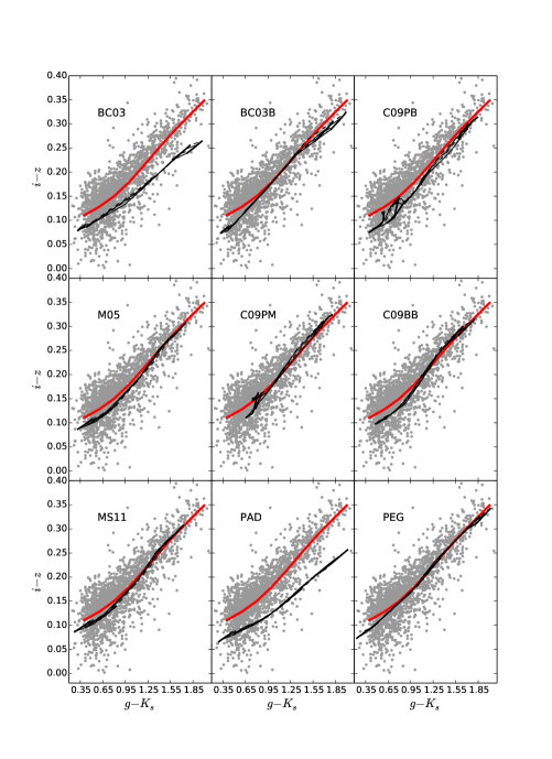
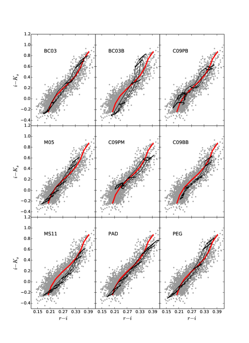
5.2. UV-optical-NIR color color diagrams
To study the effect of photometry on the relative locations of the empirical and theoretical color distributions, we use the three color-color diagrams in Figs. 15, 16, and 17.
The dynamic ranges of the synthetic , and colors agree well with the observed range. Any zero point errors compatible with our error budget (including the possible 0.04 offset in between SDSS and true AB magnitudes) would be small on the scale of the figures, and would not affect any conclusion in this section.
The diagram (Fig. 17) confirms that the spectral region around the band is matched best by models built with the MILES spectral library (C09PM and MS11). The magnitude is used in the two colors that define this diagram, exacerbating the discrepancies already seen in (Fig. 10). The majority of the models lack flux in at a given and .
The locus of the empirical color distribution is very tight both in the and in the diagrams, and this is reflected in the model grids. As in previous diagrams, there are some irregularities in the predictions of the C09 models at low metallicities, that can be traced back to their internal interpolation procedures. Only a subset of the models predicts that the addition of the band helps break the age-metallicity degeneracy. According to MS11, this would be best done in the diagram, while other models predict that the degeneracy is best broken in .
In summary, while many model colors are roughly satisfactory, none of the theoretical sets we have examined, over the range of ages and compositions we have explored, satisfactorily matches the well-defined locus of the Virgo clusters in all the color-color diagrams. Each model grid has its strengths and weaknesses in the above comparison, and we have not found strong arguments to favour one over the others overall.
5.3. Spectral Energy Distributions
While a color-color diagram provides only two colors but for all GC ages and metallicities, one SED allows a view of a set of possible colors but for only one GC (of given metallicity and age).
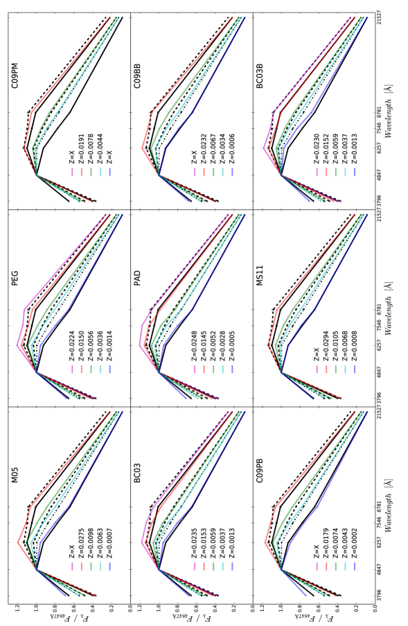
In Figure 18 we compare the fiducial SEDs of Virgo core globular clusters defined in Section 3.5, with nine sets of synthetic energy distributions for 10 Gyr-old stellar populations. The SEDs shown correspond to a given set of colors : [0.6 = Blue, 1.0 = Cyan, 1.2 = Green, 1.6 = Red, 1.8 = Magenta]. The metallicity associated with each of the plotted models is also given, to facilitate the comparison between models.
A quick overview of these theoretical SEDs confirms the wide range of fluxes that different models can predict. These discrepancies between models and observations, which easily reach 10 %, were expected based on the inspection of the color-color diagrams. They are larger at high metallicities than in the low metallicity regime. At low metallicities, models that match the bluest colors tend to match also the rest of the SED. But this does not mean that the matching models all have the same metallicity. As an extreme example, is obtained with C09PB at and with PEG or BC03 at . The MILES-based model MS11 is intermediate.
Some sets of models do not reach values as high as 1.8 mag for the metallicities we have computed (in those cases less than five model SEDs are shown in Fig. 18). Our nine model grids extend to [Fe/H] = 0.17. For five of these, this is not sufficient to reach at an age of 10 Gyr. The reason why is not reached with C09PM is only that these models are not available below [Fe/H] = -1.39.
In the color-color diagrams of Section 5.1, we had highlighted two main patterns: the relatively blue indices for the PAD and BC03 models at high metallicity, and the larger band flux relative to and in the C09PM and MS11 models. Both patterns can be seen in the SEDs, by inspecting the slope of the colored lines between and , or the energy distributions.
6. Discussion
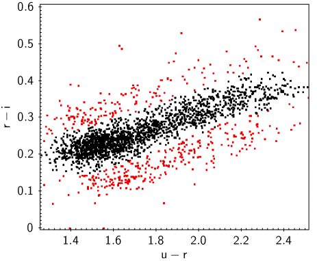
6.1. SLR calibration
The comparison of the observed GC colors with models in Section 5 is based on the data calibration against SDSS and UKIDSS (Section 2.4). Here we briefly discuss the effect of adopting, instead, the Stellar Locus Regression against synthetic stellar AB photometry (Section 2.6).
The amplitude of the SLR color-corrections based on the PHOENIX library of stellar spectra and on stellar parameters from the Besançon model of the Milky Way, is consistent with our budget of systematic errors for and , but not for and . Although the PHOENIX spectral library, combined with the Besançon model, performs better than the other libraries we have tested, we must keep in mind that it is only an approximate representation of the true stellar colors. Following High et al. (2009), we have avoided using the band in the calculation of SLR color-corrections. We have however included the band. The large SLR corrections to and are driven by the stellar locus in the three last panels of Fig. 2. At a given (bottom panels), the data must be shifted to redder and to match the synthetic stellar locus. Then the plot of versus requires a significant shift in .
The SLR color-correction vector, , points towards redder colors for all color indices. Taken at face value this suggests the dereddening corrections we have applied to the data might be excessive. The amplitude of , however, is much larger than allowed by our estimated maximal uncertainties on A(V). In and the amplitude is even larger than the total reddening towards the Virgo core region. We doubt this correction would be correct.
Based on the above, we prefer the initial calibration of the data, and restrict the discussion of the effects of the SLR to a few main trends. The re-calibrated data are compared with model grids in various color-color diagrams in Figure 23 of the Appendix.
The SLR corrections bring the Virgo core GC data closer to the models in the diagram and in the diagram (in the latter, one has to keep in mind that SDSS advocates 0.02 mag be subtracted from magnitudes). The SLR-corrected colors seem to be too red compared to the models in the and diagrams.
In any analysis of cluster properties, the main effect of using SLR-corrected colors would be a higher metallicity estimate. After the SLR-correction, more of the red GCs find no match in the model grids, and the models at [Fe/H] = -2 lie outside the distribution of observed colors. For a further discussion of GC metallicities, we refer the reader to a following paper (Powalka et al., in preparation).
6.2. Isochrones and libraries
The synthetic colors of globular cluster models depend on the assumed stellar evolution prescriptions, the resulting isochrones, and the adopted stellar spectral libraries. Our choice of models allows us to re-evaluate the validity of these ingredients in defining the colors of GCs in the Virgo core region.
The C09PB and the C09BB models of Conroy et al. (2009) respectively use Padova 2007 and BaSTI 2007 isochrones. This modification mainly affects the metal poor GCs in the , and diagrams (Figs. 10, 11 and 12), with resulting differences in color that reach 0.05 magnitudes. With that population synthesis code, the Padova 2007 isochrones produce a wider spread in colors than the BaSTI 2007 isochrones. The BC03 model can also be computed with two different sets of isochrones, which are Padova isochrones from 1993-1994 (shown in our figures) and Padova isochrones of Girardi et al. (2000), not shown). The resulting differences are below 0.05 magnitudes in all the colors in our diagrams.
Now turning to the spectral libraries, we can quantify the effects of replacing the BaSeL library with the MILES library at optical wavelengths, by comparing C09PB and C09PM in the diagram (Fig. 10). The offset in is about 0.05 magnitudes. Between BC03 and BC03B in the same diagram, the effect is of similar amplitude for red clusters, but smaller than in the Conroy implementation for blue clusters. In the diagram however (Fig. 12) the replacement of one library with the other has larger impact in the implementation of Bruzual & Charlot than with the code of Conroy et al. Here, the critical issue is the algorithm used to connect the purely optical MILES spectra with those of the panchromatic BaSeL one.
The PEG and BC03B predictions are based on very similar ingredients, and in general they agree rather well (color-color diagrams, and SEDs of Fig. 18). Differences in the details show the impact of particular implementation choices. Examples are the interpolation scheme between the few metallicities for which Padova isochrones are available, the interpolations between the spectra available in the original BaSeL library, or the detailed treatment of the TP-AGB. These numerous differences are known to produce significant effects on spectra, and make it very difficult to trace back differences in colors to a single physical origin (see Koleva et al. 2008 for a discussion of these subtle effects on the analysis of Milky Way globular cluster spectra).
Our inspection of the various models in color-color space does not allow us to point to a single “best model” that would, within the range of ages and metallicities we have considered, match the shapes and locations of the empirical distributions in all projections in a statistically acceptable way. However, we confirm that the careful flux calibration of the MILES library improves the modelling of optical spectra over pre-existing libraries. The BaSeL library on the other hand has the interesting property that it helps reaching the reddest colors seen at high metallicity in the Virgo core region, i.e. around M87. Direct consequences of the adopted stellar evolution prescriptions are smaller, or at least more difficult to isolate, than these effects of the spectral libraries.
6.3. Width of the NGVS GC distribution
The width of the locus of the GCs in the multi-dimensional color space is larger than can be explained by the random photometric errors. Several physical causes probably all contribute to this dispersion to some degree.
First, the observed GCs may have a range of ages. As we have shown in various color-color diagrams, the age-metallicity degeneracy is strong and the dispersion expected from ages spread between 6 and 13 Gyr is insufficient to explain the dispersion in the observed GC colors. One way to broaden the predicted distribution is to include ages younger than 6 Gyr. Indeed, a fraction of the clusters in the core of Virgo might have been born in relatively recent gas-rich interaction events, as a side-effect of the hierarchical merging that progressively built up the stellar mass in the center of the galaxy cluster.
The stochastic sampling of the stellar mass function in each cluster is another source of natural dispersion at a given age and metallicity. The clusters selected in this paper are massive ( M⊙), hence these stochastic effects are small. Based on models by Fouesneau & Lançon (2010), we find that they would be strongest in colors involving the and the filters, and that they remain of the order of 0.01 magnitude or less for the ages and masses of interest here. This does not suffice to explain the observed color spread.
To obtain even more variety, we may invoke more complex star formation histories than a single chemically homogeneous star formation episode, or reconsider other simplifying assumptions of the models. In the Milky Way, the assumption of a single age and a chemically homogeneous stellar population breaks down for essentially all the massive globular clusters that have been studied in detail. Hence it is likely that massive clusters in Virgo would also host more complex populations than we have assumed here.
Internal spreads in age and metallicity by themselves lead to modified integrated colors. Changes in abundance ratios significantly add to this diversity, for instance via the effects of CNO abundances on molecular bands in red giant spectra, or via the effects of helium abundances on horizontal branch temperatures. The models of Maraston & Strömbäck (2011) with a blue horizontal branch do not explain the observed colors as a whole better than the models with a red horizontal branch. Using toy models constructed with Pégase, for which we artificially varied the temperature of horizontal branch stars, we reach the same conclusion. On the other hand recent HST-based UV studies of M87 established the presence of hot stellar populations in its globular clusters (Sohn et al. 2006 and Bellini et al. 2015), which is an indication for the presence of hot horizontal branch stars. Consequently, a mix of horizontal branch morphologies is likely to contribute to the dispersion in colors we have seen. Similarly, varying fractions of blue stragglers, or stellar rotation statistics, or strong changes in the stellar mass function will spread out the colors.
Finally, we note our GC sample in the Virgo core region combines objects located around M87, around smaller Virgo galaxies such as M86 or NGC 4438, and in the intracluster region of the Virgo core. The detailed properties of each of these subpopulations differ, indicating a link with environment that we will describe in a subsequent article (Powalka et al., in preparation). Previous studies hinted at systematic differences between GC subsets. For instance, Harris (2009) showed that the typical color of the blue subsample of clusters around elliptical galaxies depends both on the distance to the galaxy center and on the GC luminosity, and Forte et al. (2013) suggest the blue and red GC subpopulations of M87 follow distinct color-color relations. The respective role of age, metallicity and additional parameters in explaining these remains to be clarified.
6.4. Stellar population properties derived from colors
The well-defined color-locus of the brightest Virgo core GCs has allowed us to illustrate the amplitude of the variation in the predictions from different sSSP models. Nevertheless, colors will remain easier to measure than spectra for remote objects in the universe, and it therefore remains desirable to provide color-based estimates of stellar population properties such ages and metallicities.
In a subsequent paper, we will present SP properties of the Virgo core clusters based on a Bayesian analysis (Powalka et al., in preparation). Using five colors that cover wavelengths from the to , we find that the metallicities derived using each of the SSP models listed in this paper individually, can differ systematically from one another by up to 0.5 dex. An analysis that combines several models allows to narrow the range of likely values significantly, although the accuracy remains dependent on the absolute adequacy of the selected models. The population synthesis models themselves clearly require more work in the future.
7. Conclusions
In this paper, we have used the Next Generation Virgo Survey to provide near-ultraviolet to near-infrared colors for a representative sample of luminous GCs in the Virgo core. The sample was selected in a plane that combines the color information of the diagram and a compactness index, measured on the NGVS images with the best seeing ( band). This hybrid plane separates globular clusters from foreground stars and background galaxies. Careful aperture corrections were applied to remove any systematic differences in colors due to seeing-variations between camera pointings.
The selection was designed to provide precise colors across the spectrum rather than ensure volume completeness. Hence the 1846 objects in the catalog are relatively bright objects, with typical masses just above M⊙. The catalog defines a characteristic locus in color-color space, from which we derive fiducial SEDs that will be useful for future quick comparisons with other samples141414Detailed studies should use the full catalog rather than the fit..
As an accurate photometric zero point is essential for comparisons with other data sets or with model predictions, we have decided to provide and test two calibrations. The first is based on a set of stars common between SDSS and NGVS, or between UKIDSS and NGVS-IR for the near-infrared. The second calibration is computed using a PHOENIX synthetic stellar library as a reference locus (Stellar Locus Regression). The PHOENIX library nicely matches the shape of the NGVS stellar locus (better than other libraries we have tested). However, residual differences between empirical and theoretical colors in the regime of low mass M dwarfs drive suspiciously large zero point corrections in and . Hence we prefer the first calibration.
To quantify the accuracy of our photometry, we have also assessed the systematic errors in the GC data. They primarily reflect uncertainties in the zero points of SDSS and UKIDSS, as well as uncertainties in the extinction towards the Virgo core. Our random errors on the mean colors along the GC color distributions are negligible compared to the systematic errors.
Accounting for our random errors, we have shown that the GC locus in color-color space cannot be explained by a single line. The width of the observed color-distribution is real. Part of this spread could be due to age differences. Other potential causes for the spread include varying binary fractions between clusters, varying stellar rotation statistics, the co-existence of sub-populations of stars with different surface chemistries within each cluster, or the presence of subsets of clusters with different chemical peculiarities in our sample. We will link color differences to the cluster environment in future work.
In the second part of this paper, we have compared the colors in our globular cluster catalog with 11 commonly used models for single age, single composition stellar populations, with ages between 6 and 13 Gyr and [Fe/H] between and 0.17. Despite a rough global agreement, we have shown that none of the 11 models provides a statistically satisfactory match to the NGVS data. Moreover, this comparison has highlighted patterns in the predictions around the and bands which are likely related to the choice of stellar spectral library made in the models.
Finally, we have not provided in this paper any ranking of the models based on their ability to match the Virgo core GC data. This ranking would depend on the exact set of colors used in the assessment, and also on the method used to measure goodness-of-fit. More importantly, it would convey the misleading impression that we recommend using one particular model and discarding the others. The ability of any of the models to represent the data is currently too imperfect to justify such a radical approach. Also, we will show in subsequent work that GCs in other environments than the Virgo core may have different color distributions, thus requiring a new assessment of the models.
We hope that these data will help for future studies and to do so, we make them available in the catalog service of the Centre de Données astronomiques de Strasbourg (CDS).
Appendix A Aperture corrections
Figure 19 illustrates the spatial distribution of the aperture corrections applied in the band. Note that this figure differs from the one in Liu et al. (2015a). Here, each star is colored using the difference between magnitudes in two SExtractor apertures, without attaching the “infinite” aperture estimate to SDSS PSF-magnitudes (as was done in the figure of Liu et al. 2015a). The varying ranges of the color scales of the four panels shows that the average aperture correction differs between pointings, due to differences in average seeing. Similar amplitudes of spatial patterns, and a similar spread between pointings, are seen in the other photometric passbands, with one exception in the band described below.
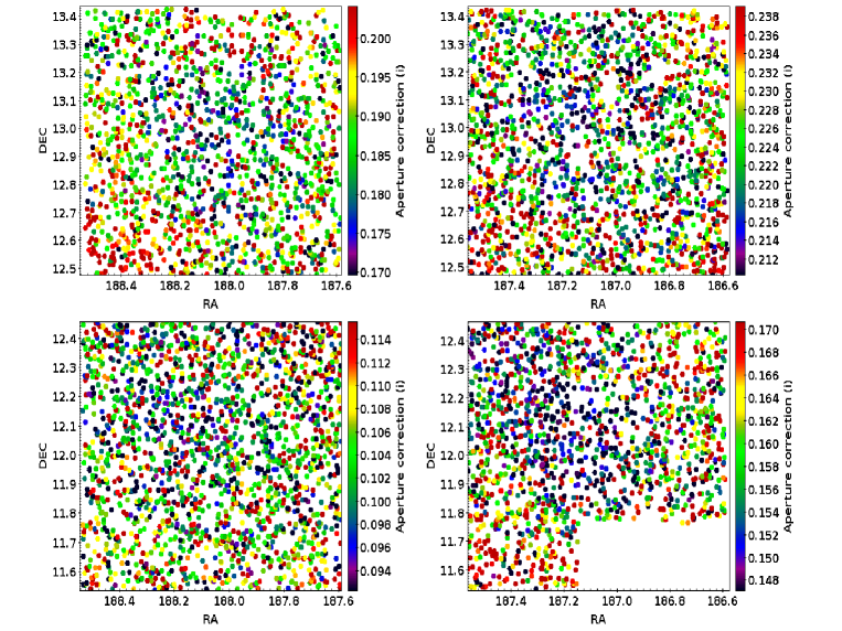
Figure 21 shows the aperture correction in NGVS pointing +0+0 (Ferrarese et al., 2012) in the band. In this one particular case, unfortunately, the seeing distribution of individual stacked images was much broader than usual. As a consequence, aperture corrections within the gaps between rows of detector chips differ more from neighbouring values than in typical cases.
Figure 21 maps the aperture corrections for photometry across the 34 WIRCam pointings of the NGVS pilot field (). Seeing differences between WIRCam pointings are the dominant cause of structure in this map, hence the distribution is comparable to the seeing maps shown in Fig. 8 of Muñoz et al. (2014).
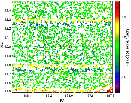
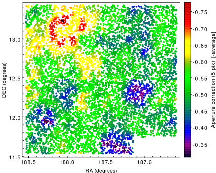
Appendix B Complementary information on the SLR calibration
B.1. UV issues
The band raises stronger calibration issues than the others when using SLR (High et al., 2009). The transmission extends across the Balmer jump of stellar spectra. In this region, spectra are particularly sensitive to stellar parameters such as temperature, gravity and also metallicity. This is seen clearly in the locus of the synthetic stars in color-color planes involving .
Figure 22 shows the effective temperature sequences of synthetic stars at a given surface gravity, for five metallicities (red : [Fe/H] = 0.0, blue : -0.5, green : -1, magenta : -1.5, cyan = -2), in six such color-color diagrams. These sequences illustrate the large sensitivity of the colors to metallicity, especially at low effective temperatures (red end of the sequences), thus creating a strong dependence on the assumed distribution of metallicities along the observed sequence (i.e. the model for the M dwarf population of the Milky Way disk and halo). Figure 2 in this paper already showed that the colors of the lower main sequence are also highly dependent on the adopted collection of theoretical spectra; this remains true for the band.
The thick black line in Figure 22 shows the locus defined by the Besançon model of the Milky Way towards Virgo. While the match to the NGVS data (shifted here by the vector of SLR shifts obtained when including in the optimization) seems reasonable to the eye, an examination of the actual scales of the offsets to the locus of the Virgo stars is alarming: they amount several tenths of a magnitude in places. In the or the diagram, the preferred model locus does not have a shape compatible with the observed stellar locus, which indicates that either the filter transmissions involved are not known well enough or the stellar models, including the choice of stellar parameters along the sequence, are not optimal. In view of the estimated uncertainties on the filter transmissions, the latter reason is believed to be predominant.
As a consequence, we have not used in the calculation of SLR corrections for GCs.
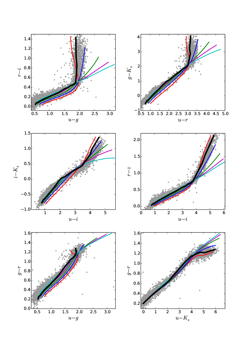
B.2. GC color-color diagrams based on the SLR calibration
The SLR-based shifts move the NGVS colors of globular colors (and other objects) to redder values. Four color-color diagrams obtained with the SLR calibration are shown in Fig. 23, and briefly discussed in Section 6.1.
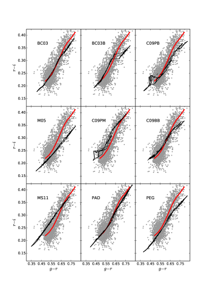
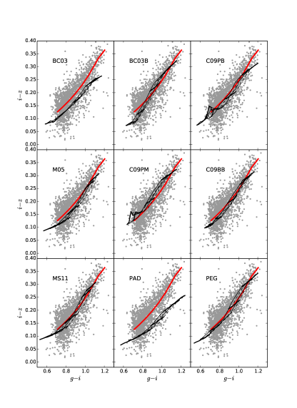
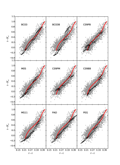
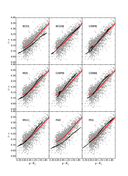
Appendix C Additional Color-Color diagrams
For the convenience of future comparison with other data sets, we provide two additional color-color diagrams in Figure 24. Like those discussed in the main body of the article, they are based on the calibration against external catalogs, described in Section 2.4.
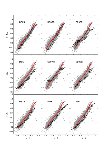
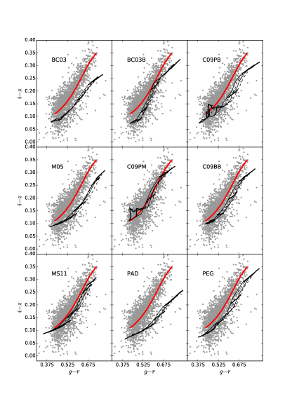
References
- Ahn et al. (2014) Ahn, C. P., Alexandroff, R., Allende Prieto, C., Anders, F., Anderson, S. F., Anderton, T., Andrews, B. H., Aubourg, É., Bailey, S., Bastien, F. A., & et al. 2014, ApJS, 211, 17
- Allard et al. (2003) Allard, F., Guillot, T., Ludwig, H.-G., Hauschildt, P. H., Schweitzer, A., Alexander, D. R., & Ferguson, J. W. 2003, in IAU Symposium, Vol. 211, Brown Dwarfs, ed. E. Martín, 325
- Alongi et al. (1993) Alongi, M., Bertelli, G., Bressan, A., Chiosi, C., Fagotto, F., Greggio, L., & Nasi, E. 1993, A&AS, 97, 851
- Bedin et al. (2004) Bedin, L. R., Piotto, G., Anderson, J., Cassisi, S., King, I. R., Momany, Y., & Carraro, G. 2004, ApJ, 605, L125
- Bellini et al. (2015) Bellini, A., Renzini, A., Anderson, J., Bedin, L. R., Piotto, G., Soto, M., Brown, T. M., Milone, A. P., Sohn, S. T., & Sweigart, A. V. 2015, ApJ, 805, 178
- Bertin & Arnouts (1996) Bertin, E., & Arnouts, S. 1996, A&AS, 117, 393
- Bertin et al. (2002) Bertin, E., Mellier, Y., Radovich, M., Missonnier, G., Didelon, P., & Morin, B. 2002, in Astronomical Society of the Pacific Conference Series, Vol. 281, Astronomical Data Analysis Software and Systems XI, ed. D. A. Bohlender, D. Durand, & T. H. Handley, 228
- Betoule et al. (2013) Betoule, M., Marriner, J., Regnault, N., Cuillandre, J.-C., Astier, P., Guy, J., Balland, C., El Hage, P., Hardin, D., Kessler, R., Le Guillou, L., Mosher, J., Pain, R., Rocci, P.-F., Sako, M., & Schahmaneche, K. 2013, A&A, 552, A124
- Bielby et al. (2012) Bielby, R., Hudelot, P., McCracken, H. J., Ilbert, O., Daddi, E., Le Fèvre, O., Gonzalez-Perez, V., Kneib, J.-P., Marmo, C., Mellier, Y., Salvato, M., Sanders, D. B., & Willott, C. J. 2012, A&A, 545, A23
- Binggeli et al. (1985) Binggeli, B., Sandage, A., & Tammann, G. A. 1985, AJ, 90, 1681
- Blakeslee et al. (2012) Blakeslee, J. P., Cho, H., Peng, E. W., Ferrarese, L., Jordán, A., & Martel, A. R. 2012, ApJ, 746, 88
- Bohlin & Gilliland (2004) Bohlin, R. C., & Gilliland, R. L. 2004, AJ, 127, 3508
- Boulade et al. (2003) Boulade, O., Charlot, X., Abbon, P., Aune, S., Borgeaud, P., Carton, P.-H., Carty, M., Da Costa, J., Deschamps, H., Desforge, D., Eppellé, D., Gallais, P., Gosset, L., Granelli, R., Gros, M., de Kat, J., Loiseau, D., Ritou, J.-., Roussé, J. Y., Starzynski, P., Vignal, N., & Vigroux, L. G. 2003, in Society of Photo-Optical Instrumentation Engineers (SPIE) Conference Series, Vol. 4841, Instrument Design and Performance for Optical/Infrared Ground-based Telescopes, ed. M. Iye & A. F. M. Moorwood, 72–81
- Bramich & Freudling (2012) Bramich, D. M., & Freudling, W. 2012, MNRAS, 424, 1584
- Bressan et al. (1993) Bressan, A., Fagotto, F., Bertelli, G., & Chiosi, C. 1993, A&AS, 100, 647
- Bressan et al. (2012) Bressan, A., Marigo, P., Girardi, L., Salasnich, B., Dal Cero, C., Rubele, S., & Nanni, A. 2012, MNRAS, 427, 127
- Bruzual & Charlot (2003) Bruzual, G., & Charlot, S. 2003, MNRAS, 344, 1000
- Cantiello & Blakeslee (2007) Cantiello, M., & Blakeslee, J. P. 2007, ApJ, 669, 982
- Cardelli et al. (1989) Cardelli, J. A., Clayton, G. C., & Mathis, J. S. 1989, ApJ, 345, 245
- Carretta et al. (2010) Carretta, E., Bragaglia, A., Gratton, R. G., Recio-Blanco, A., Lucatello, S., D’Orazi, V., & Cassisi, S. 2010, A&A, 516, A55
- Carter et al. (2008) Carter, D., Goudfrooij, P., Mobasher, B., Ferguson, H. C., Puzia, T. H., Aguerri, A. L., Balcells, M., Batcheldor, D., Bridges, T. J., Davies, J. I., Erwin, P., Graham, A. W., Guzmán, R., Hammer, D., Hornschemeier, A., Hoyos, C., Hudson, M. J., Huxor, A., Jogee, S., Komiyama, Y., Lotz, J., Lucey, J. R., Marzke, R. O., Merritt, D., Miller, B. W., Miller, N. A., Mouhcine, M., Okamura, S., Peletier, R. F., Phillipps, S., Poggianti, B. M., Sharples, R. M., Smith, R. J., Trentham, N., Tully, R. B., Valentijn, E., & Verdoes Kleijn, G. 2008, ApJS, 176, 424
- Casali et al. (2007) Casali, M., Adamson, A., Alves de Oliveira, C., Almaini, O., Burch, K., Chuter, T., Elliot, J., Folger, M., Foucaud, S., Hambly, N., Hastie, M., Henry, D., Hirst, P., Irwin, M., Ives, D., Lawrence, A., Laidlaw, K., Lee, D., Lewis, J., Lunney, D., McLay, S., Montgomery, D., Pickup, A., Read, M., Rees, N., Robson, I., Sekiguchi, K., Vick, A., Warren, S., & Woodward, B. 2007, A&A, 467, 777
- Cassisi et al. (1997a) Cassisi, S., Castellani, M., & Castellani, V. 1997a, A&A, 317, 108
- Cassisi et al. (2000) Cassisi, S., Castellani, V., Ciarcelluti, P., Piotto, G., & Zoccali, M. 2000, MNRAS, 315, 679
- Cassisi et al. (1997b) Cassisi, S., degl’Innocenti, S., & Salaris, M. 1997b, MNRAS, 290, 515
- Castelli & Kurucz (2004) Castelli, F., & Kurucz, R. L. 2004, ArXiv Astrophysics e-prints
- Chen et al. (2015) Chen, Y., Bressan, A., Girardi, L., Marigo, P., Kong, X., & Lanza, A. 2015, MNRAS, 452, 1068
- Chen et al. (2014) Chen, Y., Girardi, L., Bressan, A., Marigo, P., Barbieri, M., & Kong, X. 2014, MNRAS, 444, 2525
- Conroy et al. (2009) Conroy, C., Gunn, J. E., & White, M. 2009, ApJ, 699, 486
- Cordier et al. (2007) Cordier, D., Pietrinferni, A., Cassisi, S., & Salaris, M. 2007, AJ, 133, 468
- Côté et al. (2004) Côté, P., Blakeslee, J. P., Ferrarese, L., Jordán, A., Mei, S., Merritt, D., Milosavljević, M., Peng, E. W., Tonry, J. L., & West, M. J. 2004, ApJS, 153, 223
- Côté et al. (2001) Côté, P., McLaughlin, D. E., Hanes, D. A., Bridges, T. J., Geisler, D., Merritt, D., Hesser, J. E., Harris, G. L. H., & Lee, M. G. 2001, ApJ, 559, 828
- Coupon et al. (2009) Coupon, J., Ilbert, O., Kilbinger, M., McCracken, H. J., Mellier, Y., Arnouts, S., Bertin, E., Hudelot, P., Schultheis, M., Le Fèvre, O., Le Brun, V., Guzzo, L., Bardelli, S., Zucca, E., Bolzonella, M., Garilli, B., Zamorani, G., Zanichelli, A., Tresse, L., & Aussel, H. 2009, A&A, 500, 981
- Durrell et al. (2014) Durrell, P. R., Côté, P., Peng, E. W., Blakeslee, J. P., Ferrarese, L., Mihos, J. C., Puzia, T. H., Lançon, A., Liu, C., Zhang, H., Cuillandre, J.-C., McConnachie, A., Jordán, A., Accetta, K., Boissier, S., Boselli, A., Courteau, S., Duc, P.-A., Emsellem, E., Gwyn, S., Mei, S., & Taylor, J. E. 2014, ApJ, 794, 103
- Dye et al. (2006) Dye, S., Warren, S. J., Hambly, N. C., Cross, N. J. G., Hodgkin, S. T., Irwin, M. J., Lawrence, A., Adamson, A. J., Almaini, O., Edge, A. C., Hirst, P., Jameson, R. F., Lucas, P. W., van Breukelen, C., Bryant, J., Casali, M., Collins, R. S., Dalton, G. B., Davies, J. I., Davis, C. J., Emerson, J. P., Evans, D. W., Foucaud, S., Gonzales-Solares, E. A., Hewett, P. C., Kendall, T. R., Kerr, T. H., Leggett, S. K., Lodieu, N., Loveday, J., Lewis, J. R., Mann, R. G., McMahon, R. G., Mortlock, D. J., Nakajima, Y., Pinfield, D. J., Rawlings, M. G., Read, M. A., Riello, M., Sekiguchi, K., Smith, A. J., Sutorius, E. T. W., Varricatt, W., Walton, N. A., & Weatherley, S. J. 2006, MNRAS, 372, 1227
- Fagotto et al. (1994a) Fagotto, F., Bressan, A., Bertelli, G., & Chiosi, C. 1994a, A&AS, 104, 365
- Fagotto et al. (1994b) —. 1994b, A&AS, 105, 29
- Ferrarese et al. (2012) Ferrarese, L., Côté, P., Cuillandre, J.-C., Gwyn, S. D. J., Peng, E. W., MacArthur, L. A., Duc, P.-A., Boselli, A., Mei, S., Erben, T., McConnachie, A. W., Durrell, P. R., Mihos, J. C., Jordán, A., Lançon, A., Puzia, T. H., Emsellem, E., Balogh, M. L., Blakeslee, J. P., van Waerbeke, L., Gavazzi, R., Vollmer, B., Kavelaars, J. J., Woods, D., Ball, N. M., Boissier, S., Courteau, S., Ferriere, E., Gavazzi, G., Hildebrandt, H., Hudelot, P., Huertas-Company, M., Liu, C., McLaughlin, D., Mellier, Y., Milkeraitis, M., Schade, D., Balkowski, C., Bournaud, F., Carlberg, R. G., Chapman, S. C., Hoekstra, H., Peng, C., Sawicki, M., Simard, L., Taylor, J. E., Tully, R. B., van Driel, W., Wilson, C. D., Burdullis, T., Mahoney, B., & Manset, N. 2012, ApJS, 200, 4
- Fioc & Rocca-Volmerange (1997) Fioc, M., & Rocca-Volmerange, B. 1997, A&A, 326, 950
- Fitzpatrick (1999) Fitzpatrick, E. L. 1999, PASP, 111, 63
- Forte et al. (2005) Forte, J. C., Faifer, F., & Geisler, D. 2005, MNRAS, 357, 56
- Forte et al. (2013) Forte, J. C., Faifer, F. R., Vega, E. I., Bassino, L. P., Smith Castelli, A. V., Cellone, S. A., & Geisler, D. 2013, MNRAS, 431, 1405
- Fouesneau & Lançon (2010) Fouesneau, M., & Lançon, A. 2010, A&A, 521, A22
- Galleti et al. (2004) Galleti, S., Federici, L., Bellazzini, M., Fusi Pecci, F., & Macrina, S. 2004, A&A, 416, 917
- Geisler et al. (1996) Geisler, D., Lee, M. G., & Kim, E. 1996, AJ, 111, 1529
- Girardi et al. (2000) Girardi, L., Bressan, A., Bertelli, G., & Chiosi, C. 2000, A&AS, 141, 371
- Girardi et al. (1996) Girardi, L., Bressan, A., Chiosi, C., Bertelli, G., & Nasi, E. 1996, A&AS, 117, 113
- Girardi et al. (2010) Girardi, L., Williams, B. F., Gilbert, K. M., Rosenfield, P., Dalcanton, J. J., Marigo, P., Boyer, M. L., Dolphin, A., Weisz, D. R., Melbourne, J., Olsen, K. A. G., Seth, A. C., & Skillman, E. 2010, ApJ, 724, 1030
- Goudfrooij et al. (2009) Goudfrooij, P., Puzia, T. H., Kozhurina-Platais, V., & Chandar, R. 2009, AJ, 137, 4988
- Gratton et al. (2004) Gratton, R., Sneden, C., & Carretta, E. 2004, ARA&A, 42, 385
- Gullieuszik et al. (2008) Gullieuszik, M., Held, E. V., Rizzi, L., Girardi, L., Marigo, P., Momany, Y., Saviane, I., & Ortolani, S. 2008, Mem. Soc. Astron. Italiana, 79, 427
- Gustafsson et al. (2008) Gustafsson, B., Edvardsson, B., Eriksson, K., Jørgensen, U. G., Nordlund, Å., & Plez, B. 2008, A&A, 486, 951
- Hanes et al. (2001) Hanes, D. A., Côté, P., Bridges, T. J., McLaughlin, D. E., Geisler, D., Harris, G. L. H., Hesser, J. E., & Lee, M. G. 2001, ApJ, 559, 812
- Harris (1996) Harris, W. E. 1996, AJ, 112, 1487
- Harris (2009) —. 2009, ApJ, 703, 939
- Hewett et al. (2006) Hewett, P. C., Warren, S. J., Leggett, S. K., & Hodgkin, S. T. 2006, MNRAS, 367, 454
- High et al. (2009) High, F. W., Stubbs, C. W., Rest, A., Stalder, B., & Challis, P. 2009, AJ, 138, 110
- Hodgkin et al. (2009) Hodgkin, S. T., Irwin, M. J., Hewett, P. C., & Warren, S. J. 2009, MNRAS, 394, 675
- Husser et al. (2013) Husser, T.-O., Wende-von Berg, S., Dreizler, S., Homeier, D., Reiners, A., Barman, T., & Hauschildt, P. H. 2013, A&A, 553, A6
- Huxor et al. (2014) Huxor, A. P., Mackey, A. D., Ferguson, A. M. N., Irwin, M. J., Martin, N. F., Tanvir, N. R., Veljanoski, J., McConnachie, A., Fishlock, C. K., Ibata, R., & Lewis, G. F. 2014, MNRAS, 442, 2165
- Ilbert et al. (2006) Ilbert, O., Arnouts, S., McCracken, H. J., Bolzonella, M., Bertin, E., Le Fèvre, O., Mellier, Y., Zamorani, G., Pellò, R., Iovino, A., Tresse, L., Le Brun, V., Bottini, D., Garilli, B., Maccagni, D., Picat, J. P., Scaramella, R., Scodeggio, M., Vettolani, G., Zanichelli, A., Adami, C., Bardelli, S., Cappi, A., Charlot, S., Ciliegi, P., Contini, T., Cucciati, O., Foucaud, S., Franzetti, P., Gavignaud, I., Guzzo, L., Marano, B., Marinoni, C., Mazure, A., Meneux, B., Merighi, R., Paltani, S., Pollo, A., Pozzetti, L., Radovich, M., Zucca, E., Bondi, M., Bongiorno, A., Busarello, G., de La Torre, S., Gregorini, L., Lamareille, F., Mathez, G., Merluzzi, P., Ripepi, V., Rizzo, D., & Vergani, D. 2006, A&A, 457, 841
- Jordán et al. (2007) Jordán, A., Blakeslee, J. P., Côté, P., Ferrarese, L., Infante, L., Mei, S., Merritt, D., Peng, E. W., Tonry, J. L., & West, M. J. 2007, ApJS, 169, 213
- Jordán et al. (2005) Jordán, A., Côté, P., Blakeslee, J. P., Ferrarese, L., McLaughlin, D. E., Mei, S., Peng, E. W., Tonry, J. L., Merritt, D., Milosavljević, M., Sarazin, C. L., Sivakoff, G. R., & West, M. J. 2005, ApJ, 634, 1002
- Jordán et al. (2009) Jordán, A., Peng, E. W., Blakeslee, J. P., Côté, P., Eyheramendy, S., Ferrarese, L., Mei, S., Tonry, J. L., & West, M. J. 2009, ApJS, 180, 54
- Kinman (1959) Kinman, T. D. 1959, MNRAS, 119, 538
- Koleva et al. (2008) Koleva, M., Prugniel, P., Ocvirk, P., Le Borgne, D., & Soubiran, C. 2008, MNRAS, 385, 1998
- Kroupa (1998) Kroupa, P. 1998, MNRAS, 298, 231
- Kroupa (2001) —. 2001, MNRAS, 322, 231
- Kundu & Whitmore (2001) Kundu, A., & Whitmore, B. C. 2001, AJ, 121, 2950
- Lawrence et al. (2007) Lawrence, A., Warren, S. J., Almaini, O., Edge, A. C., Hambly, N. C., Jameson, R. F., Lucas, P., Casali, M., Adamson, A., Dye, S., Emerson, J. P., Foucaud, S., Hewett, P., Hirst, P., Hodgkin, S. T., Irwin, M. J., Lodieu, N., McMahon, R. G., Simpson, C., Smail, I., Mortlock, D., & Folger, M. 2007, MNRAS, 379, 1599
- Le Borgne et al. (2004) Le Borgne, D., Rocca-Volmerange, B., Prugniel, P., Lançon, A., Fioc, M., & Soubiran, C. 2004, A&A, 425, 881
- Le Borgne et al. (2003) Le Borgne, J.-F., Bruzual, G., Pelló, R., Lançon, A., Rocca-Volmerange, B., Sanahuja, B., Schaerer, D., Soubiran, C., & Vílchez-Gómez, R. 2003, A&A, 402, 433
- Lejeune et al. (1997) Lejeune, T., Cuisinier, F., & Buser, R. 1997, A&AS, 125, 229
- Lejeune et al. (1998) —. 1998, A&AS, 130, 65
- Liu et al. (2015a) Liu, C., Peng, E. W., Côté, P., Ferrarese, L., Jordán, A., Mihos, J. C., Zhang, H.-X., Muñoz, R. P., Puzia, T. H., Lançon, A., Gwyn, S., Cuillandre, J.-C., Blakeslee, J. P., Boselli, A., Durrell, P. R., Duc, P.-A., Guhathakurta, P., MacArthur, L. A., Mei, S., Sánchez-Janssen, R., & Xu, H. 2015a, ApJ, 812, 34
- Liu et al. (2015b) Liu, C., Peng, E. W., Toloba, E., Mihos, J. C., Ferrarese, L., Alamo-Martínez, K., Zhang, H.-X., Côté, P., Cuillandre, J.-C., Cunningham, E. C., Guhathakurta, P., Gwyn, S., Herczeg, G., Lim, S., Puzia, T. H., Roediger, J., Sánchez-Janssen, R., & Yin, J. 2015b, ApJ, 812, L2
- Lokhorst et al. (2016) Lokhorst, D., Starkenburg, E., McConnachie, A. W., Navarro, J. F., Ferrarese, L., Côté, P., Liu, C., Peng, E. W., Gwyn, S. D. J., Cuillandre, J.-C., & Guhathakurta, P. 2016, ApJ, 819, 124
- Lotz et al. (2004) Lotz, J. M., Miller, B. W., & Ferguson, H. C. 2004, ApJ, 613, 262
- Maraston (2005) Maraston, C. 2005, MNRAS, 362, 799
- Maraston & Strömbäck (2011) Maraston, C., & Strömbäck, G. 2011, MNRAS, 418, 2785
- Marigo & Girardi (2007) Marigo, P., & Girardi, L. 2007, A&A, 469, 239
- Marigo et al. (2008) Marigo, P., Girardi, L., Bressan, A., Groenewegen, M. A. T., Silva, L., & Granato, G. L. 2008, A&A, 482, 883
- McCracken et al. (2010) McCracken, H. J., Capak, P., Salvato, M., Aussel, H., Thompson, D., Daddi, E., Sanders, D. B., Kneib, J.-P., Willott, C. J., Mancini, C., Renzini, A., Cook, R., Le Fèvre, O., Ilbert, O., Kartaltepe, J., Koekemoer, A. M., Mellier, Y., Murayama, T., Scoville, N. Z., Shioya, Y., & Tanaguchi, Y. 2010, ApJ, 708, 202
- Mei et al. (2007) Mei, S., Blakeslee, J. P., Côté, P., Tonry, J. L., West, M. J., Ferrarese, L., Jordán, A., Peng, E. W., Anthony, A., & Merritt, D. 2007, ApJ, 655, 144
- Melbourne et al. (2012) Melbourne, J., Williams, B. F., Dalcanton, J. J., Rosenfield, P., Girardi, L., Marigo, P., Weisz, D., Dolphin, A., Boyer, M. L., Olsen, K., Skillman, E., & Seth, A. C. 2012, ApJ, 748, 47
- Muñoz et al. (2014) Muñoz, R. P., Puzia, T. H., Lançon, A., Peng, E. W., Côté, P., Ferrarese, L., Blakeslee, J. P., Mei, S., Cuillandre, J.-C., Hudelot, P., Courteau, S., Duc, P.-A., Balogh, M. L., Boselli, A., Bournaud, F., Carlberg, R. G., Chapman, S. C., Durrell, P., Eigenthaler, P., Emsellem, E., Gavazzi, G., Gwyn, S., Huertas-Company, M., Ilbert, O., Jordán, A., Läsker, R., Licitra, R., Liu, C., MacArthur, L., McConnachie, A., McCracken, H. J., Mellier, Y., Peng, C. Y., Raichoor, A., Taylor, M. A., Tonry, J. L., Tully, R. B., & Zhang, H. 2014, ApJS, 210, 4
- Oldham & Auger (2016) Oldham, L. J., & Auger, M. W. 2016, MNRAS, 455, 820
- Padmanabhan et al. (2008) Padmanabhan, N., Schlegel, D. J., Finkbeiner, D. P., Barentine, J. C., Blanton, M. R., Brewington, H. J., Gunn, J. E., Harvanek, M., Hogg, D. W., Ivezić, Ž., Johnston, D., Kent, S. M., Kleinman, S. J., Knapp, G. R., Krzesinski, J., Long, D., Neilsen, Jr., E. H., Nitta, A., Loomis, C., Lupton, R. H., Roweis, S., Snedden, S. A., Strauss, M. A., & Tucker, D. L. 2008, ApJ, 674, 1217
- Paudel et al. (2013) Paudel, S., Duc, P.-A., Côté, P., Cuillandre, J.-C., Ferrarese, L., Ferriere, E., Gwyn, S. D. J., Mihos, J. C., Vollmer, B., Balogh, M. L., Carlberg, R. G., Boissier, S., Boselli, A., Durrell, P. R., Emsellem, E., MacArthur, L. A., Mei, S., Michel-Dansac, L., & van Driel, W. 2013, ApJ, 767, 133
- Peng et al. (2006) Peng, E. W., Jordán, A., Côté, P., Blakeslee, J. P., Ferrarese, L., Mei, S., West, M. J., Merritt, D., Milosavljević, M., & Tonry, J. L. 2006, ApJ, 639, 95
- Pickles (1998) Pickles, A. J. 1998, PASP, 110, 863
- Pietrinferni et al. (2004) Pietrinferni, A., Cassisi, S., Salaris, M., & Castelli, F. 2004, ApJ, 612, 168
- Piotto (2007) Piotto, G. 2007, Highlights of Astronomy, 14, 434
- Piotto et al. (2012) Piotto, G., Milone, A. P., Anderson, J., Bedin, L. R., Bellini, A., Cassisi, S., Marino, A. F., Aparicio, A., & Nascimbeni, V. 2012, ApJ, 760, 39
- Pota et al. (2013) Pota, V., Graham, A. W., Forbes, D. A., Romanowsky, A. J., Brodie, J. P., & Strader, J. 2013, MNRAS, 433, 235
- Puzia et al. (2002) Puzia, T. H., Zepf, S. E., Kissler-Patig, M., Hilker, M., Minniti, D., & Goudfrooij, P. 2002, A&A, 391, 453
- Raichoor & Andreon (2012) Raichoor, A., & Andreon, S. 2012, A&A, 537, A88
- Raichoor et al. (2014) Raichoor, A., Mei, S., Erben, T., Hildebrandt, H., Huertas-Company, M., Ilbert, O., Licitra, R., Ball, N. M., Boissier, S., Boselli, A., Chen, Y.-T., Côté, P., Cuillandre, J.-C., Duc, P. A., Durrell, P. R., Ferrarese, L., Guhathakurta, P., Gwyn, S. D. J., Kavelaars, J. J., Lançon, A., Liu, C., MacArthur, L. A., Muller, M., Muñoz, R. P., Peng, E. W., Puzia, T. H., Sawicki, M., Toloba, E., Van Waerbeke, L., Woods, D., & Zhang, H. 2014, ApJ, 797, 102
- Renzini et al. (2015) Renzini, A., D’Antona, F., Cassisi, S., King, I. R., Milone, A. P., Ventura, P., Anderson, J., Bedin, L. R., Bellini, A., Brown, T. M., Piotto, G., van der Marel, R. P., Barbuy, B., Dalessandro, E., Hidalgo, S., Marino, A. F., Ortolani, S., Salaris, M., & Sarajedini, A. 2015, MNRAS, 454, 4197
- Renzini & Fusi Pecci (1988) Renzini, A., & Fusi Pecci, F. 1988, ARA&A, 26, 199
- Robin et al. (2003) Robin, A. C., Reylé, C., Derrière, S., & Picaud, S. 2003, A&A, 409, 523
- Robin et al. (2004) —. 2004, A&A, 416, 157
- Rosenfield et al. (2014) Rosenfield, P., Marigo, P., Girardi, L., Dalcanton, J. J., Bressan, A., Gullieuszik, M., Weisz, D., Williams, B. F., Dolphin, A., & Aringer, B. 2014, ApJ, 790, 22
- Sánchez-Blázquez et al. (2006) Sánchez-Blázquez, P., Peletier, R. F., Jiménez-Vicente, J., Cardiel, N., Cenarro, A. J., Falcón-Barroso, J., Gorgas, J., Selam, S., & Vazdekis, A. 2006, MNRAS, 371, 703
- Sanchez-Janssen et al. (2016) Sanchez-Janssen, R., Ferrarese, L., MacArthur, L. A., Cote, P., Blakeslee, J. P., Cuillandre, J.-C., Duc, P.-A., Durrell, P., Gwyn, S., McConnachie, A. W., Boselli, A., Courteau, S., Emsellem, E., Mei, S., Peng, E., Puzia, T. H., Roediger, J., Simard, L., Boyer, F., & Santos, M. 2016, ArXiv e-prints
- Schlafly & Finkbeiner (2011) Schlafly, E. F., & Finkbeiner, D. P. 2011, ApJ, 737, 103
- Schlegel et al. (1998) Schlegel, D. J., Finkbeiner, D. P., & Davis, M. 1998, ApJ, 500, 525
- Searle et al. (1980) Searle, L., Wilkinson, A., & Bagnuolo, W. G. 1980, ApJ, 239, 803
- Sohn et al. (2006) Sohn, S. T., O’Connell, R. W., Kundu, A., Landsman, W. B., Burstein, D., Bohlin, R. C., Frogel, J. A., & Rose, J. A. 2006, AJ, 131, 866
- Stetson et al. (1989) Stetson, P. B., Hesser, J. E., Smith, G. H., Vandenberg, D. A., & Bolte, M. 1989, AJ, 97, 1360
- Strader et al. (2011) Strader, J., Romanowsky, A. J., Brodie, J. P., Spitler, L. R., Beasley, M. A., Arnold, J. A., Tamura, N., Sharples, R. M., & Arimoto, N. 2011, ApJS, 197, 33
- Tamura et al. (2006) Tamura, N., Sharples, R. M., Arimoto, N., Onodera, M., Ohta, K., & Yamada, Y. 2006, MNRAS, 373, 601
- Tang et al. (2014) Tang, J., Bressan, A., Rosenfield, P., Slemer, A., Marigo, P., Girardi, L., & Bianchi, L. 2014, MNRAS, 445, 4287
- Usher et al. (2015) Usher, C., Forbes, D. A., Brodie, J. P., Romanowsky, A. J., Strader, J., Conroy, C., Foster, C., Pastorello, N., Pota, V., & Arnold, J. A. 2015, MNRAS, 446, 369
- Vazdekis et al. (2012) Vazdekis, A., Ricciardelli, E., Cenarro, A. J., Rivero-González, J. G., Díaz-García, L. A., & Falcón-Barroso, J. 2012, MNRAS, 424, 157
- Westera et al. (2002) Westera, P., Lejeune, T., Buser, R., Cuisinier, F., & Bruzual, G. 2002, A&A, 381, 524
- Yoon et al. (2006) Yoon, S.-J., Yi, S. K., & Lee, Y.-W. 2006, Science, 311, 1129
- Zhang et al. (2015) Zhang, H.-X., Peng, E. W., Côté, P., Liu, C., Ferrarese, L., Cuillandre, J.-C., Caldwell, N., Gwyn, S. D. J., Jordán, A., Lançon, A., Li, B., Muñoz, R. P., Puzia, T. H., Bekki, K., Blakeslee, J. P., Boselli, A., Drinkwater, M. J., Duc, P.-A., Durrell, P., Emsellem, E., Firth, P., & Sánchez-Janssen, R. 2015, ApJ, 802, 30
- Zinn (1985) Zinn, R. 1985, ApJ, 293, 424