Accelerating scientific codes by
performance and accuracy modeling

Abstract

Scientific software is often driven by multiple parameters that affect both accuracy and performance. Since finding the optimal configuration of these parameters is a highly complex task, it extremely common that the software is used suboptimally. In a typical scenario, accuracy requirements are imposed, and attained through suboptimal performance. In this paper, we present a methodology for the automatic selection of parameters for simulation codes, and a corresponding prototype tool. To be amenable to our methodology, the target code must expose the parameters affecting accuracy and performance, and there must be formulas available for error bounds and computational complexity of the underlying methods. As a case study, we consider the particle-particle particle-mesh method (PPPM) from the LAMMPS suite for molecular dynamics, and use our tool to identify configurations of the input parameters that achieve a given accuracy in the shortest execution time. When compared with the configurations suggested by expert users, the parameters selected by our tool yield reductions in the time-to-solution ranging between 10% and 60%. In other words, for the typical scenario where a fixed number of core-hours are granted and simulations of a fixed number of timesteps are to be run, usage of our tool may allow up to twice as many simulations. While we develop our ideas using LAMMPS as computational framework and use the PPPM method for dispersion as case study, the methodology is general and valid for a range of software tools and methods.

1 Introduction

Simulation software is often governed by a number of parameters that affect both the accuracy of the results and the time-to-solution. In a typical setting, the choice of these values represents a challenging trade-off scenario: the more accuracy is desired, the more computation is required (thus longer simulations), and vice versa. Users, who normally aim at a target accuracy level, face the problem of choosing $p$, a configuration of the parameters (i.e., a tuple of values), on a given set of computing resources, that fulfills the accuracy requirements while minimizing the execution time:

$$\min_{p}\ \text{time}(\text{resources},p)\quad\text{subject to}\quad\text{accurate}(p).$$

The problem is exacerbated by the large space of possibilities, the intricate relation among the parameters, and the dependence on the actual simulated system and underlying architecture. In general, given the dimensionality of the space of configurations, finding the optimal values for the parameters is a daunting task, and even experts necessitate a considerable amount of trial and error to only provide rules of thumb that often are suboptimal. Users are left with two options: either use the (potentially) suboptimal rules of thumb from the literature, or perform a tedious and time consuming search, which requires knowledge from the application domain, the solver, and the underlying computing architecture. In this paper, we present a methodology for the automatic parameter selection for simulation codes, aiming at both an increase in productivity and an improved utilization of computing resources of scientific simulations. A case study on one of the most popular methods in molecular dynamics (the particle-particle particle-mesh method PPPM-Hockney ) demonstrates the potential savings offered by the methodology.

To be amenable to our methodology, a numerical code must present the following three characteristics. First, it has to be governed by a number of parameters that affect the efficiency of the computation and/or the accuracy of the results; these parameters must be exposed to the user, typically as input arguments to the simulation software. Second, analytical formulas as functions of the parameters need to be available for the estimation of the error incurred by a given configuration. Finally, rough (asymptotic) cost estimates, generated either manually or analytically, are required. If these three requirements are satisfied, the methodology proceeds in three steps.

1. The first step consists in characterizing the parameters that represent the search space; this involves identifying those parameters that affect performance and/or accuracy, choosing meaningful ranges for them, and discretizing the continuous ones. We refer to the set of all possible values for these parameters as the “parameter space” or “search space”.

2. In the second step, analytical error bounds are used to divide the search space into accurate and inaccurate configurations, according to whether or not they are estimated to satisfy the user requirements; only the accurate subspace is further considered.

3. As a third step, the execution time of the method is modeled by fitting one or more functions corresponding to the computational cost of the method to data samplings (collected from short runs); the combination of these functions yields a model that accurately predicts the execution time for each configuration in the accurate subspace.

The description of the steps of the methodology is deliberately general. In practice, their application will be adjusted to the properties of the method to overcome the curse of dimensionality: While the first stage only requires acquiring a high-level understanding of the method or software at hand, the second and third stages require actual computation, and the potentially high dimensionality of the search space poses challenges to an accurate prediction and selection of parameters. To overcome these challenges, it is critical to exploit method-specific properties and knowledge in order to reduce the complexity of the search and to obtain faster and more accurate predictions.

To illustrate the potential of the methodology, we developed a prototype that implements the methodology and applied it to the particle-particle particle-mesh (PPPM) method. This method is governed by four parameters (three of them affect performance, and all four affect accuracy) leading to a large parameter space. Moreover, the overall accuracy of the simulation may be regulated by multiple accuracy thresholds, corresponding to different sections of the method. In general, in order to remove the need for a manual search of good configurations and to simplify the user’s workflow, the developers of the solvers provide rules of thumb on how to set these parameters. However, since the optimal choice highly depends on both the actual simulation and the architecture, the effectiveness of these guidelines is limited. In contrast, as we demonstrate, when both the simulated system and the computing architecture are taken into account, it is possible to identify configurations that lead to close-to-optimal performance, and thus to an efficient use of resources.

The benefits of our tool are two-fold. On the one hand, it provides the users with close-to-optimal configurations specifically chosen for the system and architecture of interest. On the other hand, it does so while dispensing them from the burden of an unpleasant and time-consuming manual search for such efficient configurations. Moreover, the tool does not require any deep understanding of the solvers or computing architectures. The user can thus focus on the high-level aspects of the scientific problem.

In short, our experiments demonstrate how even expert choices for parameters might be severely suboptimal in terms of efficiency: While the simulations deliver the required accuracy, they do not do so in the most efficient way. In other words, resources are underutilized. At the expense of an initial (automated) search, our approach yields gains in terms of productivity and better usage of resources. This is especially relevant in the common cases where the simulations take considerable time or many simulations with similar characteristics are to be run. More specifically, in our experiments we observed reductions of time-to-solution between 10% and 60%. Given the length of typical molecular dynamics simulations, this may translate to savings of hours or even days of computation, or the execution of twice as many simulations given a fixed core-hour budget.

1.1 Contributions.

The main contribution of this paper is a methodology for the automatic parameter selection for simulation software. The requirements for its application are that the parameters affecting accuracy and performance of the software are exposed to the user, and that formulas for error bounds and computational complexity of the underlying solvers are available. The outcome of the process is a configuration of the parameters that yields accurate enough results in (almost) minimal time. We focus on the domain of molecular dynamics, and contribute a practical example of the potential benefits of our approach based on a very popular method in the field, the particle-particle particle-mesh method (pppm) PPPM-Hockney , and its implementation from the well-known LAMMPS suite LAMMPS-1995 . Usage of our prototype implementing the methodology does not require deep knowledge of the solvers and computing architectures, and at the cost of an easily amortized automated search, the tool provides the user with close-to-optimal configurations. As a result, researchers are enabled to carry out many more or larger simulations and therefore to gain deeper scientific insights in the problem at hand.

1.2 Outline of the paper.

This paper is structured as follows. Section 2 provides an overview of the basic ideas behind molecular dynamics and the PPPM method. Sections 3, 4 and 5 discuss in detail the three steps in our methodology, with practical examples using the PPPM method. These steps are: characterization of the search space, identification of the accurate subspace, and sampling and modeling. In Sec. 6 we present multiple experimental results, while in Sec. 7 we draw conclusions.

2 Background

This section reviews the basic ideas behind molecular dynamics and the PPPM method, as well as research efforts related to the presented work. The readers familiar with both molecular dynamics and PPPM may skip this section.

2.1 Molecular Dynamics and the PPPM method

Molecular dynamics (MD) is a well-established tool for the study of the properties of complex particle systems at the atomistic level; it is widely used in a variety of fields, including computational chemistry, biophysics, and materials science. Typical simulations consist of systems comprising between thousands and tens of millions of particles. In order to simulate time scales relevant for the processes being studied, and thus to obtain meaningful evidence, these systems must evolve for at least millions of timesteps. In practice, MD simulations are limited by computing resources, and practitioners usually have to apply for compute time on supercomputers. It is therefore critical to make an efficient use of the available resources.

The basic idea underlying an MD simulation is to study the movement of the particles due to the forces acting on each of them, for a given time span. The computation in these simulations is dominated by the calculation of the forces exerted on each particle (or, similarly, the calculation of the potential energy of the system). Given a system with $n$ particles, the direct evaluation of pairwise interactions would cost $O(n^{2})$ operations (per timestep), and is thus entirely infeasible for systems with a large number of particles. The so-called mesh-based Ewald methods, among which we find the PPPM method, reduce the algorithmic complexity to $O(n\,\,log\,n)$ PPPM-Hockney ; PME-Darden ; SPME-Essmann .

In order to reduce the computational cost of one timestep from $O(n^{2})$ to $O(n\,log\,n)$, PPPM splits the the interactions into short- and long-range ones. Forces among neighboring particles within a given cutoff radius are computed in real space by means of direct evaluation, while forces due to the interaction of distant particles are computed in Fourier (or reciprocal) space. The calculation of the reciprocal space contributions, that is, the long-range interactions, requires solving the Poisson equation in Fourier space. In order to take advantage of the Fast-Fourier Transform (FFT) algorithm and achieve the $O(n\,log\,n)$ complexity, the potential of the particles is mapped into a regular grid, computations based on FFTs are performed, and the resulting potential is mapped back to the particles. Depending on the specifics of how the Poisson equation is solved, multiple flavors of PPPM arise. In the following, we consider two of them: analytical differentiation ($ad$), and $i$k numerical differentiation ($i$k). For details on these two flavors we refer the reader to MeshUpI .

A simulation based on the PPPM method is governed by 4 parameters: the cutoff, which restricts the short-range contribution to particles within a certain radius; the size of the grid into which the particles are mapped for the calculations of the long-range interactions; the interpolation order, which affects the mapping of potential into the grid, and indicates the number of grid points (per dimension) to which the potential is mapped; and the Ewald parameter, which controls the weight of each (short- and long-range) contribution. Out of these four parameters, the first three (cutoff, grid size, and interpolation order) affect both the accuracy and execution time of the simulation, while the Ewald parameter affects the accuracy but not the execution time.

The impact of the cutoff, grid size, and interpolation order is rather straightforward. When the cutoff is increased, more particles are taken into consideration, the accuracy of the real space part also increases, and the computation becomes more expensive. Similarly, an increase in the grid size or in the interpolation order results in higher accuracy and computational cost for the reciprocal space part. The role of the Ewald parameter ($\alpha$) is more subtle. While it does not play a role in terms of computation, and thus performance, it has a strong influence on accuracy. For instance, for a fixed cutoff, grid, and interpolation order, larger values of $\alpha$ improve the accuracy of the real space and reduce that of the reciprocal space. This fact can be used to optimize performance: Given a configuration that attains the desired accuracy but is suboptimal in terms of performance, the value of $\alpha$ can be modified to shift the contribution to compute time from one part to the other.

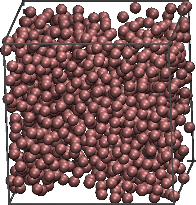
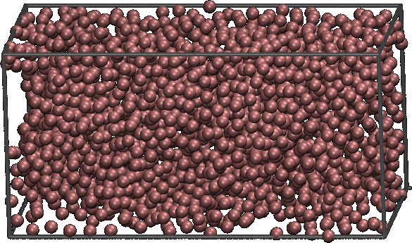
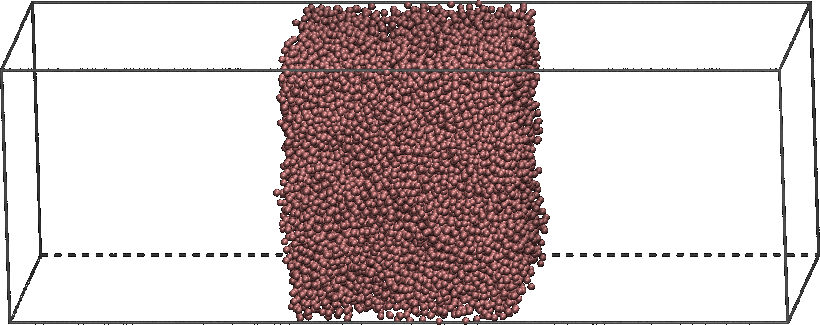
To showcase our methodology, we choose the two types of systems depicted in Fig. 1: bulk (homogeneous) and interfacial (inhomogeneous). Homogeneous systems, with a random distribution of particles over the entire domain, are typically used to initially test accuracy, and performance models. Inhomogeneous systems are very common and the most relevant in practice; they constitute a class of complex enough systems to stress the effectiveness of our methodology.

Figure 1: Two types of systems. Left, bulk system. Right, interfacial system.

As a specific implementation of the PPPM solver, we choose the PPPM solver for dispersion interactions from the LAMMPS package, a widely-used open source MD suite. The choice of the solver for dispersion is not arbitrary; dispersion forces are a type of forces that exist between all types of atoms and are therefore present in every system. Of course, our approach is applicable to other types of forces, such as the electrostatic ones.

Our tool takes as input a description of the simulation to be run and the desired accuracy, and returns as output the estimated fastest configuration that satisfies the accuracy constraints. The input description includes the size of the simulation domain, the number of particles in the domain, and whether they fill up the entire domain (bulk), or only a box within the domain (interfacial). The desired accuracy is expressed as either two independent thresholds for the short- and long-range contributions ($\Delta F_{real}$ and $\Delta F_{reciprocal}$, respectively), or a single value as a threshold for the combined root mean square ($\sqrt{\Delta F_{real}^{2}+\Delta F_{reciprocal}^{2}}$ ), where $\Delta F_{\star}$ is defined as $\sqrt{\frac{1}{N}\sum_{i=1}^{N}(F_{i}-F_{i}^{\text{exact}})^{2}}$, $N$ the number of particles. The tool returns the estimated optimal values for cutoff, grid size, interpolation order, and Ewald parameter.

2.2 Related work

Research efforts in the domain of molecular dynamics simulations concentrate mainly in the design of accurate and efficient methods and their parallel scalable implementation in software packages. The MD landscape is populated with a broad variety of methods, from simple truncation (with or without tail correction), through tree methods, and grid-based methods. The latter group contains, among others, the particle-mesh Ewald (PME), smooth particle-mesh Ewald (SPME), the particle-particle particle-mesh (PPPM), and the multi-level summation (MSM) methods. Our methodology is applicable to all these methods.

The list of available molecular dynamics suites is also large. Among others, it is worth mentioning GROMACS, NAMD, and CHARMM. GROMACS-1995 ; CHARMM-2009 ; NAMD While in our case study we consider LAMMPS, the approach is generic and totally portable to any other suite.

Literature on the accuracy of the different methods is abundant Kolafa1992 ; Petersen1995 ; Deserno:1998wb ; Hardy2006 . Furthermore, there exists literature on the optimal choice of certain parameters for accuracy. Among them, in MeshUpII , the authors discuss the choice of optimal Ewald parameter given fixed cutoff, grid size, and interpolation order for the PPPM method in its $i$k differentiation flavor. The authors of Stern-optimal-ewald perform a similar study for both $ad$ and $i$k differentiation in PPPM. However, despite the importance of making an efficient usage of the available resources in order to target larger systems, the optimal choice of parameters in terms of performance has received much less attention. An attempt that shares some resemblance with our approach is given in Wang-optimal-perf . They propose an analytical approach to finding optimal values for all four parameters in SPME (the same four as in PPPM). However, we observe two limitations in the study. First, the fact that their approach does not take into consideration the actual hardware. The authors work under the assumption that every flop (arithmetic operation) has the same cost; due to caching effects and the cost of data movement, it is well understood that an accurate model requires taking into account that the cost of flops is not constant across a piece of software. Second, their numerical results do not provide any reference to understand how close the execution times are to the optimal. As later discussed in this paper, we determine the region in the parameter space that potentially contains the optimal configurations, and compare the results of our tool with the best timings in that region. The fact that we take into consideration the architecture, also allows to identify close-to-optimal configurations across computing platforms.

3 Characterization of the search space

The first step in our methodology for the automatic selection of parameters is to characterize the parameter space, that is, to identify the set of parameters $\mathcal{P}$ that play a role in the accuracy and/or performance of the target method.

For most algorithms in computational science, the set $\mathcal{P}$ of input parameters is a mixture of (potentially unbounded) discrete and continuous values. For each of these parameters, a range must be specified and, for the continuous ones, a discretization (not necessarily regular) provided. This process originates the search space $\mathcal{S}$ of parameter configurations. Without loss of generality, when there is freedom in the choice, the granularity of the discretization and the considered ranges of values are set based on the experience of practitioners and domain experts.

The objective of our methodology is to find the configuration, that is, the one point in the (highly dimensional) space $\mathcal{S}$, that delivers the requested accuracy in the minimum time.

Example: Characterizing $\mathcal{S}$ for the pppm method. The pppm method is parameterized by the cutoff radius ($r_{c}$), the grid size ($(n_{x}\times n_{y}\times n_{z})$), the interpolation order ($p$), and the Ewald parameter ($\alpha$). Out of the four parameters, the interpolation order and the grid size are already discrete, while the Ewald parameter and the cutoff are continuous. In the LAMMPS implementation of pppm, the accepted values for the interpolation order are integers from 2 to 6. The grid size is restricted to values that can be expressed as multiples of only 2, 3, and 5 (e.g., a grid of size $60\times 60\times 60$ is valid, but not a grid of size $66\times 66\times 66$). To constrain the (infinite) number of possible grid sizes, we dynamically set an upper bound based on the system under consideration. This upper bound is limited so that only grids containing a number of grid points up to 8 times the number of particles in the system (2x per dimension) and with a shape proportional to the simulation domain are allowed. This bound is generous—the optimal grid size is typically far from the largest allowed—and may be decreased to reduce the search time.

With respect to the continuous parameters, the Ewald parameter must be strictly positive, and is typically not much larger than 1.0$\sigma^{-1}$; we allow values in the range (0.0, 1.0]. As for the cutoff, no hard constraints are imposed, other than being strictly positive; however, it is accepted that it takes at least a value of 2.0$\sigma$. Regarding the upper bound, we allow rather large cutoffs up to 6.0$\sigma$. For the discretization of the Ewald parameter and the cutoff, we choose a step size of 0.01$\sigma^{-1}$ and 0.1$\sigma$, respectively. We recall that in both cases one can certainly explore a larger space of values; the aforementioned bounds are flexible and the validity of our methodology and results are not affected by these choices.

This discretization leads to a 4-dimensional search space, where each configuration consists of a 4-tuple ($\alpha$, $r_{c}$, $(n_{x}\times n_{y}\times n_{z})$, $p$). As we discuss in the next section, the evaluation of error estimates for all configurations in $\mathcal{S}$ is computationally too expensive and thus unfeasible in practice due to the introduced overhead. Furthermore, it is expensive to develop an accurate performance model that takes the entirety of the search space into account. Therefore we advocate for an approach that exploits the structure of the target methods to reduce the dimensionality of the search. For the pppm method (and an entire class of similar methods), this includes (1) the fact that only accurate configurations are worth considering, and (2) the study of both accuracy and performance can be split using a divide-and-conquer strategy into the study of its components, namely the real- and reciprocal-space contributions, which are then composed to provide a global solution.

4 Identification of the accurate subspace

In this first computational stage of our methodology, accuracy bounds are used as a discriminant to restrict the search space to only those configurations that result in simulations accurate enough to merit the effort of performance modeling. Therefore, the discretized parameter space is split into accurate and inaccurate subspaces, $\mathcal{S_{A}}$ and $\mathcal{S_{I}}$ respectively, and only the former is kept for further consideration. We refer to the boundary between both subspaces as the frontier ($\mathcal{F}$). The frontier is a Pareto Efficient Frontier comprising the configurations that are Pareto optimal, that is, configurations that, while satisfying the accuracy constraints, cannot reduce the contribution to the computational cost of any one of the parameters without increasing the contribution of the others or without compromising the accuracy of the solution (crossing the boundary accurate-inaccurate).

To estimate the accuracy of each configuration of parameters, we require the availability of formulas for the error bounds. These are typically derived, and provided by the developer of each method in the corresponding publication. For pppm, the error bounds are provided in Rolf1 , and consist of two formulas, for the real space and the the reciprocal space contributions, respectively. We outline these formulas. The error of the real space contribution is bound by

$$\Delta F_{real}=\frac{{C}\sqrt{\pi}\alpha^{5}}{\sqrt{NVr_{c}}}\left(\frac{6}{r^{6}_{c}\alpha^{6}}+\frac{6}{r^{4}_{c}\alpha^{4}}+\frac{3}{r^{2}_{c}\alpha^{2}}+1\right)e^{-r^{2}_{c}\alpha^{2}},$$

where $C$ is the dispersion coefficient (dependent on the particles in the system), $N$ is the number of particles in the system, $V$ is the volume of the system, and $\alpha$ and $r_{c}$ are the Ewald parameter and the cutoff, respectively.

The error for the reciprocal space contribution is bound by

$$\Delta F_{reciprocal}=C\sqrt{\frac{Q}{NV}},$$

where

$$Q=\frac{1}{V}\sum_{{\bf k}\in\mathbb{M}}\left\{\sum_{{\bf m}\in\mathbb{Z}^{3}}\left|{\bf\tilde{R}}\left({\bf k}+\frac{2\pi}{h}{\bf m}\right)\right|^{2}-\frac{\left|\tilde{\bf D}({\bf k})\sum_{{\bf m}\in\mathbb{Z}^{3}}\tilde{U}^{2}({\bf k}+\frac{2\pi}{h}{\bf m})\tilde{\bf R}^{*}({\bf k}+\frac{2\pi}{h}{\bf m})\right|^{2}}{|\tilde{\bf D}({\bf k})|^{2}[\sum_{{\bf m}\in\mathbb{Z}^{3}}\tilde{U}^{2}({\bf k}+\frac{2\pi}{h}{\bf m})]^{2}}\right\}.$$

The details of the last formula are beyond the scope of this paper. The main message is that it is not uncommon that error bounds are given by means of complex formulas, whose evaluation might be computationally expensive and even require numerical approximations.

To limit the cost of the evaluation of the formulas, one can make use of the available knowledge on the specific method at hand. For instance, in pppm, since separate formulas are provided for both the real- and reciprocal-space contributions, and some of the parameters affect only one of the two errors, we decompose the evaluation in that of each space, and then combine the results to obtain the error estimates for each configuration of the four-dimensional space. This approach is general and valid for a class of methods with similar characteristics.

In pppm, the real space error is only affected by the choice of $\alpha$ and $r_{c}$, while that of the reciprocal space is only affected by the choice of $\alpha$, $p$, and $(n_{x}\times n_{y}\times n_{z})$. Figures 2(a) and 2(b) show, respectively, the independent evaluation of the error estimates for the real and reciprocal spaces. The figures correspond to the Large Cube test case (TestLC) described in Appendix A. The figures illustrate the tradeoffs and difficulties associated with the manual selection of parameters for a simulation run. While higher values of the Ewald parameter increase the real-space accuracy, they reduce the accuracy of the reciprocal space. Also, for a fixed target accuracy, smaller values of the Ewald parameter allow to use a smaller grid size or interpolation order, and hence to reduce the execution time for the reciprocal-space calculation, at the expense of setting a larger cutoff, thus increasing the execution time for the real space, and vice versa. It becomes apparent that identifying the accurate subspace $\mathcal{S_{A}}$, and then determining the fastest configurations within $\mathcal{S_{A}}$ is a daunting task.

(a) Real-space error.

(b) Reciprocal-space error.

Figure 2: Contour plots for the study of the accurate subspace. The plots correspond to TestLC using $ad$ differentiation. In the case of the reciprocal space, we show the error for an interpolation order of 5.

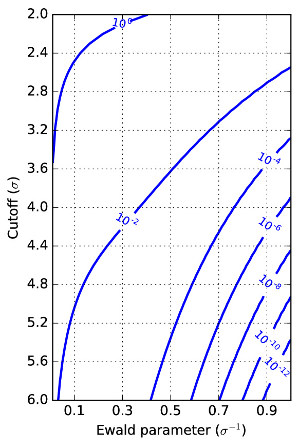
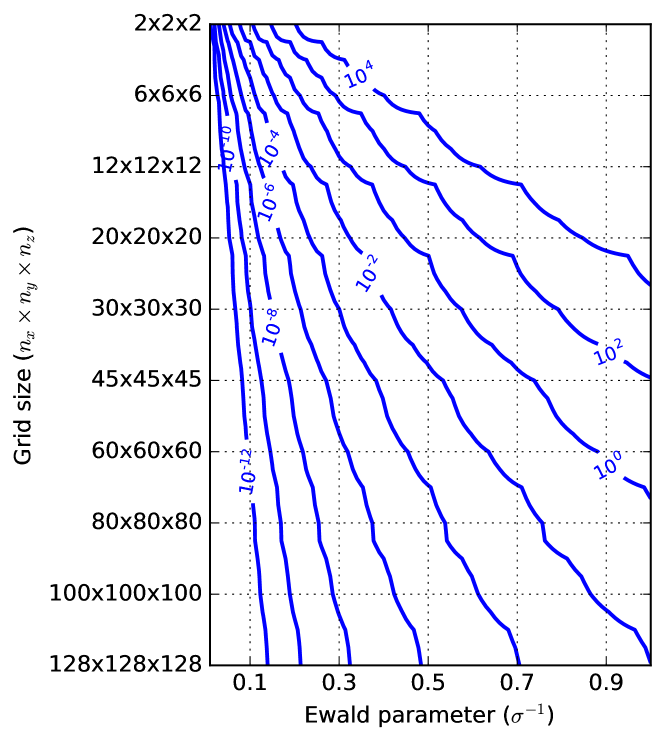
While the evaluation of the real-space error formula is inexpensive, the evaluation of the reciprocal-space error formula is, unfortunately, still too costly, even when only the 3D subspace $\alpha$ $\times$ $(n_{x}\times n_{y}\times n_{z})$ $\times$ $p$ is considered. In fact, the values for Fig. 2(b) were calculated by an approximation also provided in Rolf1 which is only valid for the $i$k differentiation, cubic domains, and grid sizes with equal number of grid points in each dimension. Without this simplification, the evaluation of the entire grid using the generalized formula would take days. We opt for an alternative that further reduces the amount of required evaluations of the formula. The insight is that it suffices to identify the values that split accurate and inaccurate configurations. That is, referring to Fig. 2(b), if the user requests an accuracy of $10^{-4}\epsilon/\sigma$, it suffices to find the corresponding contour plot; every point below that line is accurate enough. To this end, for each interpolation order and grid size, we perform a binary search for this splitting value. Additionally, the search is parallelized and carried out in place, making use of the same architecture in which the simulation will be run. Following this idea, the time spent in the evaluation of the error estimates may be reduced from days to minutes.

Once the error estimates for both real and reciprocal spaces are available, these are combined back in the single four-dimensional space $S$; it is then possible to split the full search space $\mathcal{S}$ into $S_{A}$ and $S_{I}$, according to the target accuracy. The splitting of the search space is carried out in one of two different ways, depending on how the user expresses the accuracy requirements. If the user inputs one single value for the accuracy, those configurations where the combined root mean square of the errors ($\sqrt{\Delta F_{real}^{2}+\Delta F_{reciprocal}^{2}}$ ) is below the accuracy threshold are considered. If, instead, the user provides individual thresholds for each component, then the individual errors must satisfy the corresponding constraint independently.

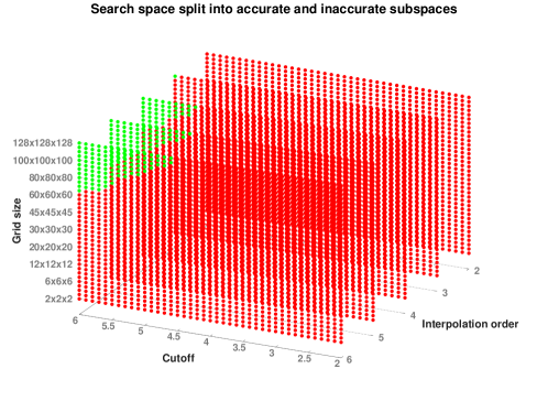
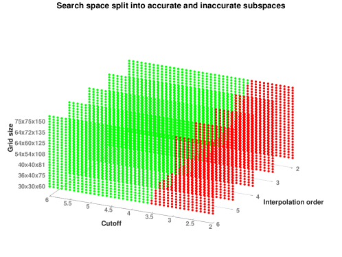
It is now important to point out that not all of the parameters that influence accuracy also impact performance. For instance, $\alpha$ only affects accuracy, and does not directly influence the amount of computation performed. Thus, the space of parameters can be reduced to 3-dimensional ($r_{c}$, $(n_{x}\times n_{y}\times n_{z})$, $p$) when modeling performance. At this stage, points in this three-dimensional space are labeled as inaccurate, unless there exists at least one value of $\alpha$ that makes the combination accurate. Figures 3 and 4 illustrate this subdivision, respectively for TestLC, and the bulk system used in our experimental results (Sec. 6). In both figures, green and red dots denote the accurate and inaccurate subspaces, respectively.

Figure 3: Search space divided into accurate and inaccurate configurations for TestLC.

Figure 4: Search space divided into accurate and inaccurate configurations for the bulk system described in Sec. 6.2.

5 Sampling and modeling

Once the accurate subspace $\mathcal{S_{A}}$ has been identified, the third and final step consists in determining the configurations in $\mathcal{S_{A}}$ that lead to the best overall performance. A range of alternatives exist to estimate the execution time given a choice of parameters. At one extreme, one could rely on a purely analytical approach which consists of using the flop count (the amount of arithmetic operations required by a given configuration) as a metric to estimate the execution time. Unfortunately, it is well-understood that not every flop incurs the same cost: Different sections of a given implementation attain different performance levels (flops/s), and even variations of the values for the parameters influence the use of the memory hierarchy (reuse of data), and thus performance. Therefore, even though flops are a metric that allows for a fast estimation of execution time, they lead to inaccurate predictions. At the other extreme, one may consider a purely empirical approach, where each of the accurate configurations is executed and timed, and the fastest one is selected. However, the number of configurations in $\mathcal{S_{A}}$ may vary from several hundred to tens of thousands, depending on the particular system and the desired accuracy. Such an extensive search would still consume considerable resources. Thus, this approach is reliable, but slow. Instead, we advocate a hybrid analytical-empirical approach, based on a reduced number of samples, which predicts the performance for each configuration by fitting a set of simple models to the measurements.

In Sec. 5.1, we present a static strategy that samples at a set of predetermined points in the space. While rather effective and useful to better understand the properties of the method, it presents some drawbacks that we discuss in Sec. 5.2. In Sec. 5.3, we switch to a dynamic sampling strategy that reduces significantly the amount of required sampling and improves the accuracy of the estimations. As our experiments confirm, the adaptive approach yields fast and reliable predictions.

5.1 Static dense sampling

Our static approach consists in collecting samples at a set of predefined points that cover a relatively dense subset of the space. The granularity of the sampling obviously affects the accuracy and speed of the prediction: the larger the number of samples, the slower and the more accurate is the prediction, and vice versa. If the space and the cost of sampling are too large, properties of the method may be exploited to, for instance, reduce the dimensionality of the space or speedup the samples.

For the pppm method, we take advantage of the fact that the method consists of two successive, independent stages, and model each stage in isolation. The resulting models are then combined to produce the predictions. Similarly to the approach taken to evaluate the analytical formulas for the error bounds, a divide-and-conquer strategy is used to decompose the performance modeling of the pppm method into that of the real and reciprocal contributions. Thus, the real and reciprocal spaces are sampled independently, the samples are then fitted to models, and finally the models are combined to predict the total compute time of the accurate configurations.

5.1.1 Sampling the real-space computation

The only parameter that affects the time required to compute the real-space contribution is the cutoff. Hence, different values for the cutoff are sampled, while the other parameters are fixed. More specifically, we use the following configurations:

• Ewald parameter: 0.50$\sigma^{-1}$

• Interpolation order: 2

• Grid size: $1\times 1\times 1$

• Cutoff: [2.0$\sigma$, 2.5$\sigma$, 3.0$\sigma$, …, 6.0$\sigma$]

Here, the choice of Ewald parameter is arbitrary, and the interpolation order and grid size are set to the smallest possible value to minimize the time spent in the sampling. We sample at multiple values of the cutoff in the range $[2.0\sigma,\ 6.0\sigma]$ in steps of 0.5$\sigma$, for a total of nine data points.

5.1.2 Sampling the reciprocal-space computation

The time spent in computing the reciprocal-space contribution is, in principle, affected only by the grid size and the interpolation order. Hence, the cutoff and Ewald parameter are fixed, and the following configurations are sampled:

• Ewald parameter: 0.50$\sigma^{-1}$

• Interpolation order: [2, 3, 4, 5, 6]

• Grid sizes: a function of the target system (domain size and number of particles)

• Cutoff: 2.0$\sigma$.

Once again, the choice of the Ewald parameter value is arbitrary, the cutoff is kept to a minimum, and we sample all interpolation orders in the range $[2,6]$, and the full set of valid grid sizes within a range determined according to the number of particles and domain size of the target system. The total number of data points varies with the size of the system, and is equal to five (interpolation orders) times the number of considered grid sizes.

Here, and for the remainder of the paper, each sampling consists in the execution of 1000 timesteps of the actual simulation of interest; of course, this number is configurable. The rest of the properties of the simulation, such as mixing rules, ensemble, temperature, etc, are fixed and configured by the user.

5.1.3 Modeling and fitting

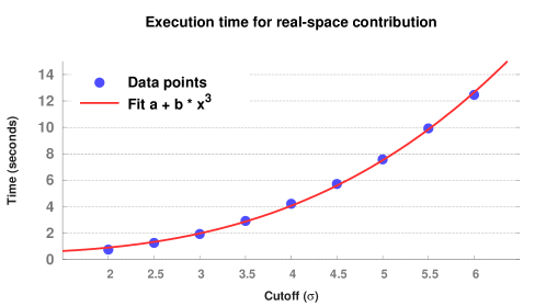
Each set of samples is now fitted to a corresponding function. The choice of the functions to be used comes either from domain expertise or from the analysis of the method’s complexity. Since the computational cost for the evaluation of the real-space contribution is proportional to the cube of the cutoff, we fit the function $f(c)=a+b\cdot c^{3}$ to the data points ($c_{i}$, $t(c_{i})$), where the parameter $a$ accounts for the overhead in allocation and setting of data. As an example, we consider the test case Small Interface (TestSI, see App. A for details). Figure 5 shows the measured execution time for the real-space contribution for each of the sampled cutoff values. The fit is satisfactory, presenting an average relative error $\frac{1}{n}\sum_{i=1}^{n}(|f(c_{i})-t(c_{i})|/t(c_{i}))$ of less than 5%.

Figure 5: Fitting of the function $f(c)=a+b*c^{3}$ to the timings for the real-space contribution in TestSI ($i$k differentiation). Values for parameters $a$ and $b$ are 0.44 and 0.0565, respectively. The average relative error is less than 5%.

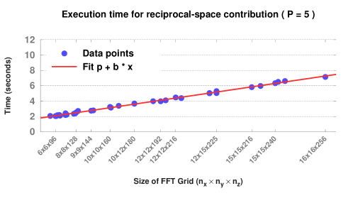
To simplify the modeling of the reciprocal space, we consider each interpolation order $P$ independently. Accordingly, we model the execution time of the reciprocal space by means of multiple functions $h_{i}(g)=p+b\cdot g$, where $g$ represents the number of points in the FFT grid, and $p$ accounts for the time spent in the mapping of the particles into the grid and back. Figure 6 depicts the execution time for the reciprocal space corresponding to $P=5$ and a range of grid sizes, also for TestSI. The average relative error is around 2%.

Figure 6: Fitting of the function $h_{5}(g)=p+b*g$ to the timings for the reciprocal-space contribution in TestSI ($i$k differentiation). Values for parameters $p$ and $b$ are 1.81 and $8.33\cdot 10^{-5}$, respectively. The average relative error is 2.3%.

5.1.4 Prediction

An estimate of the overall compute time is obtained by summing up the estimates for the real-space and the reciprocal-space contributions. We use test case TestSI to provide preliminary results on the accuracy of the predictions yielded by the described static approach. As a reference, we measured the time spent in the computation of the real and reciprocal space contributions for the frontier configurations and compared the timings with the predictions for these same points. Table 1 collects the results for the fastest five configurations based on empirical measurements (column 2). Columns 3 and 4 show the predicted execution time for those same configurations and the relative error in the prediction, measured as $|t_{pred}-t_{emp}|/t_{pred}$, where $t_{emp}$ is the empirically measured time and $t_{pred}$ is the predicted time. The model-based predictions are quite accurate. The average relative error for the entire set of frontier configurations (73) is 4.98%. Moreover, and most importantly, the methodology correctly identifies the configuration which leads to the fastest execution.

Empirical		Prediction		Configuration
Ranking	Time	Time	Error	$\alpha$	$r_{c}$	$p$	$(n_{x}\times n_{y}\times n_{z})$
#1	8.770s	8.378s	(-4.68%)	0.56$\sigma^{-1}$	4.60$\sigma$	4	$10\times 10\times 160$
#2	8.920s	8.495s	(-4.99%)	0.60$\sigma^{-1}$	4.40$\sigma$	4	$12\times 12\times 180$
#3	9.023s	8.595s	(-4.98%)	0.63$\sigma^{-1}$	4.30$\sigma$	4	$12\times 12\times 216$
#4	9.119s	8.754s	(-4.17%)	0.58$\sigma^{-1}$	4.50$\sigma$	5	$10\times 10\times 160$
#5	9.299s	8.610s	(-8.00%)	0.64$\sigma^{-1}$	4.20$\sigma$	5	$12\times 12\times 180$

Table 1: Predictions for TestSI ($i$k differentiation) using static sampling.

5.2 Advantages and disadvantages of the static sampling

We observed a number of advantages and disadvantages of using a static sampling. Among the advantages, we highlight the simplicity of implementation, since the approach is system-agnostic, that is, the system does not influence the search beyond the selection of grid sizes to consider, and no online decisions are necessary. Second, the accuracy of the predictions is rather satisfactory in general. Finally, it is relevant beyond the automatic selection of parameters. The sampling allows to understand the behavior of the method in practice and to expose unexpected performance signatures. We give examples below.

On the contrary, we also identified a number of drawbacks that may imply limited accuracy in the predictions or excessive sampling time:

1. Unexpectedly, the value of the cutoff does affect the execution time of the reciprocal-space computation.

2. Unlike in Fig. 6, in certain cases the timings for the reciprocal space may not fit a single straight line; two shifted lines are observed instead (see Fig. 8 below).

3. The number of required samples may grow large.

These issues are discussed in detail hereafter. Our proposed solution, based on adaptive sampling, is developed in the next subsection.

Impact of $r_{c}$ on the reciprocal space.

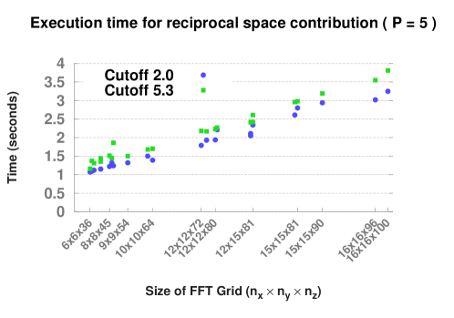
While, in principle, the cutoff should only have an impact on the execution time of the real-space contribution, we observed that the execution time of the reciprocal space is also affected. This behavior is observed, for instance, in the test case Small Bulk (TestSB, see App. A). As illustrated by Fig. 7, the difference in execution time when calculating the reciprocal-space contribution with two different fixed cutoffs (in this case 2.0$\sigma$ and 5.3$\sigma$) may be considerable. Indeed, these differences are carried on to the prediction of the execution time of the overall simulation, as illustrated in Tab. 2. Columns 3 and 4 correspond to predictions after using a cutoff of 2.0$\sigma$ for the samplings of the reciprocal-space. As one can appreciate, the predictions may be quite off. In fact, the average relative error between the measured and the estimated execution times when using this cutoff is about 5%. If, instead, we take into account the range of cutoff values represented in the configurations included in $S_{A}$, and choose to sample using a value for the cutoff within that range, the overall estimation improves. In the case of TestSB, the cutoff in the frontier configurations ranges from 4.6$\sigma$ to 6.0$\sigma$. If we fix the cutoff for sampling to the mid value (5.3$\sigma$), the average relative error (Tab. 2, columns 5 and 6) is reduced to about 2%. We thus conclude that is critical to dynamically choose the sampling values based on the simulation under consideration in order to obtain highly-accurate predictions.

Figure 7: Difference in execution time for the calculation of the reciprocal-space contribution when using different cutoffs.

Empirical		Prediction ($r_{c}$ = 2.0$\sigma$)		Prediction ($r_{c}$ = 5.3$\sigma$)
Ranking	Time	Time	Error	Time	Error
#1	7.498s	7.413s	(-1.15%)	7.679s	(+2.36%)
#2	7.542s	7.394s	(-2.01%)	7.687s	(+1.88%)
#3	7.595s	7.270s	(-4.47%)	7.610s	(+0.20%)
#4	7.660s	7.520s	(-1.86%)	7.759s	(+1.28%)
#5	7.800s	7.255s	(-7.52%)	7.736s	(-0.83%)

Table 2: Results for TestSB ($i$k differentiation). The accuracy of the predictions improve when using a cutoff closer to the range in the frontier configurations ([4.6$\sigma$, 6.0$\sigma$]).

Irregular behavior of the reciprocal space.

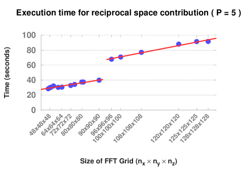
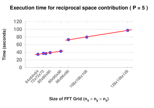
In some test cases, we observed that the timings for the reciprocal space do not lay on one single line, but rather on two parallel ones (in a piecewise manner). We relate this behavior to a switch in the data distribution in pppm’s implementation Rolf1 ; Rolf2 , where depending on the grid size and the number of processes used for the computation, the FFT domain is decomposed either in slabs (faces) or pencils (columns). More specifically, the shift occurs at the point where the number of grid points in the $z$ dimension becomes equal or greater than the number of processes used in the simulation. As an example, Fig. 8 illustrates the shift for the TestLC scenario. In the example, 96 processes where used; the shift thus occurs at grid size $96\times 96\times 96$. An adaptive sampling approach is required to identify the gap and correctly fit the data.

Figure 8: Samples for the execution time of the reciprocal-space contribution in TestLC ($ad$ differentiation). The data is not fitted by one single line; it requires two of them, with a similar slope but a shifted offset.

Reducing the number of samples.

Finally, the dense static sampling may involve a fairly large number of samples. For instance, TestSI ($i$k differentiation) requires around 200 samples. While tractable, the number of required samples will be reduced with an adaptive sampling technique.

5.3 Adaptive sampling

In light of the aforementioned issues, we present here an adaptive strategy to exploring the search space, whose decisions are guided by the characteristics of the simulation at hand.

The new strategy is built upon the algorithm sketched in Alg. 1. Given a fitting function f, the list of possible values for the independent variables xs (either the cutoff for the real space or the grids for the reciprocal space) and an error threshold, the algorithm commences by sampling the minimum, maximum, and midpoint values in xs; the function f is then fitted to the measurements. If the relative error at any of the sampled points is larger than the given threshold, the algorithm proceeds recursively for each half of xs; it terminates otherwise.

Next, we make use of a classic top-down algorithm for the segmentation of time series segmentation that takes the series of samples collected by Alg. 1 and creates a piece-wise function consisting of one or more instances of f with different parameters $a_{1},a_{2},...,a_{n}$. Six such piece-wise functions will be created, one for the real space contribution, and five for the reciprocal space (one per interpolation order). These functions will then be used to model the execution time of each contribution given a cutoff value (real space), an interpolation order and a grid size (reciprocal space).

1:function adaptive_sampling(f, threshold, xs)

2:     function adaptive_sampling_rec(i, j)

3:         if $(j-i)\leq 1$ then

4:              return

5:         end if

6:         midpoint = (i+j) / 2

7:         timings(midpoint) = sample(midpoint)

8:         x = [xs(i), xs(midpoint), xs(j)]

9:         y = [timings(i), timings(midpoint), timings(j)]

10:         if error(f, x, y) $>$ threshold then

11:              adaptive_sampling_rec(i, midpoint)

12:              adaptive_sampling_rec(midpoint, j)

13:         end if

14:     end function

15:     n_xs = length(xs)

16:     timings = array(n_xs)

17:     timings(1) = sample(1)

18:     timings(n_xs) = sample(n_xs)

19:     adaptive_sampling_rec(1, n_xs)

20:     return timings

21:end function

Algorithm 1 : Adaptive sampling.

This adaptive strategy reduces the amount of sampling. For instance, when sampling for the reciprocal space in TestSI, the static full sampling (Sec. 5.1) and the adaptive sampling use 18 and 3 data points per interpolation order, respectively (see Fig. 6 vs. Fig. 9). In the “less friendly” TestLC scenario, 17 and 8 samples per interpolation order are used, respectively (see Fig. 8 vs. Fig. 10). Not only the number of samples is reduced; the shift is also correctly identified, thus improving the accuracy of the predictions.

Finally, the effects of the cutoff in the computation of the reciprocal-space term are addressed as follows: instead of fixing the value of the cutoff to 2.0$\sigma$, we sample for the minimum and the maximum values of the cutoff present in the accurate subspace, and interpolate for intermediate values. To compensate for the increase in number of samplings, we further adjust the sampling to the target system. Concretely, since we are only interested in accurate enough configurations, we only sample the interpolation orders present in the accurate subspace configurations. Likewise, we adjust the range of grid sizes for the sampling of the reciprocal space and the range of cutoffs for the sampling of the real space.

Figure 9: Samples for the execution time of the reciprocal-space contribution in TestSI ($i$k differentiation). Dynamic strategy.

Figure 10: Samples for the execution time of the reciprocal-space contribution in TestLC ($ad$ differentiation). Dynamic strategy.

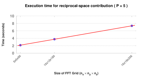
As a result of the described adaptive sampling, we obtain accurate predictions at a reduced sampling cost. In Tab. 3, we present results for TestSI ($i$k differentiation). While the static sampling required 99 samples and attained a relative error of 4.98%, the dynamic strategy only required 37 samples, and achieved a reduced relative error of 2.46%. Most importantly, the dynamic approach still selects the fastest configuration as the optimal choice.

Empirical		Prediction		Configuration
Ranking	Time	Time	Error	$\alpha$	$r_{c}$	$p$	$(n_{x}\times n_{y}\times n_{z})$
#1	8.770s	8.663s	(-1.23%)	0.56$\sigma^{-1}$	4.60$\sigma$	4	$10\times 10\times 160$
#2	8.920s	8.808s	(-1.26%)	0.60$\sigma^{-1}$	4.40$\sigma$	4	$12\times 12\times 180$
#3	9.023s	8.919s	(-1.16%)	0.63$\sigma^{-1}$	4.30$\sigma$	4	$12\times 12\times 216$
#4	9.119s	9.024s	(-1.06%)	0.58$\sigma^{-1}$	4.50$\sigma$	5	$10\times 10\times 160$
#5	9.299s	8.886s	(-4.64%)	0.64$\sigma^{-1}$	4.20$\sigma$	5	$12\times 12\times 180$

Table 3: Predictions for TestSI ($i$k differentiation) based on dynamic sampling.

Table 4 collects similar results for the TestLC scenario ($ad$ differentiation). The average relative error is of 3.72%, obtained with 51 samples. As in the previous example, our methodology again selects the fastest configuration as optimal.

Empirical		Prediction		Configuration
Ranking	Time	Time	Error	$\alpha$	$r_{c}$	$p$	$(n_{x}\times n_{y}\times n_{z})$
#1	91.663s	94.163s	(+2.65%)	0.52$\sigma^{-1}$	5.30$\sigma$	6	$90\times 90\times 90$
#2	92.356s	96.552s	(+4.35%)	0.50$\sigma^{-1}$	5.50$\sigma$	6	$80\times 80\times 80$
#3	92.374s	95.707s	(+3.48%)	0.49$\sigma^{-1}$	5.50$\sigma$	5	$90\times 90\times 90$
#4	93.417s	98.256s	(+4.93%)	0.48$\sigma^{-1}$	5.60$\sigma$	6	$75\times 75\times 75$
#5	93.675s	98.289s	(+4.69%)	0.47$\sigma^{-1}$	5.70$\sigma$	5	$80\times 80\times 80$

Table 4: Predictions for the TestLC scenario ($ad$ differentiation) based on dynamic sampling.

6 Experimental results

Through a number of case studies, we now discuss in detail the practical benefits of our methodology to speed up scientific codes. For each experiment, we report the time required by our tool to estimate the best selection of parameters, and the speedup with respect to the parameters chosen by an expert. Moreover, we quantify the benefits brought to the end user in terms of amount of additional research enabled, that is, for a characteristic setting where a scientist is granted 10 million core-hours at a supercomputer, and each simulation is to be run for 50 million timesteps, we calculate how many additional simulations are now possible.

6.1 Experimental setup

The experiments were run on two computing clusters. The first one, referred as Harpertown, consists of 32 nodes; each node comprises two four-core Intel Harpertown E5450 processors, operating at a frequency of 3.00GHz, and is equipped with 16GB of RAM. The second cluster is the SuperMUC supercomputer at the Leibniz Supercomputing Center; each node of SuperMUC consists of 16-core nodes based on Sandy Bridge-EP Xeon E5-2680 processors, operating at a frequency of 2.7GHz. Each node is equipped with 32GB of RAM. In all cases, the simulations were run using LAMMPS (version 22Jan14), FFTW, and OpenMPI.

In all cases, Lennard Jones particles with energy $\epsilon$ and diameter $\sigma$ were randomly placed in the domain (or box for interfacial systems). Then, the systems were equilibrated for 100,000 timesteps after minimization using soft potential. The simulations were run at a temperature of 0.7$\epsilon$/$k_{B}$ using a Nosé-Hoover thermostat NoseHoover with damping factor of 10$\tau$.

For the type of systems used in our experiments, the developer of the LAMMPS PPPM solver for dispersion recommends to set the target accuracy to 0.001$\epsilon/\sigma$ for the real space and 0.1$\epsilon/\sigma$ for the reciprocal space. As for a fair comparison against the parameters automatically selected by our tool, he suggests to set a cutoff value of $r_{c}=3.0\sigma$ and let the solver set the other parameters (Ewald parameter, interpolation order, and grid size).

6.2 Case Study 1: Bulk system

As a first case study, we consider a bulk system consisting of 256,000 Lennard-Jones (LJ) particles randomly placed in a domain of length $55\sigma\times 55\sigma\times 110\sigma$. The computations were carried out on 12 Harpertown nodes (i.e., 96 processors).

To determine the benefit of our methodology for automatic parameter selection, we compare it with a human expert’s best guess, and with the empirical fastest. The execution time for a sample of 1,000 timesteps with the configuration suggested by the developer is collected in Tab. 5, rows 2 and 4. The empirical fastest configurations and the corresponding timings are displayed in rows 3 and 5. Next, we allowed our prediction tool to run the necessary samples to estimate the execution time of the parameterizations at the frontier configurations, and select the predicted fastest. The sampling and prediction took about four hours. Table 5 collects the results for our tool. In both cases, the predictions match the best empirically-determined configurations. The final choice of our tool is to use $ad$ differentiation with the following parameters: ($\alpha$$\;=0.84$, $r_{c}$$\;=3.30\sigma$, $p$$\;=4$, $(n_{x}\times n_{y}\times n_{z})$$\;=45\times 45\times 90$). The choice not only coincides with the empirically fastest, but it also reduces execution time by 35% with respect to the developer’s best guess.

Approach	Diff.	Time	$\alpha$	$r_{c}$	$p$	$(n_{x}\times n_{y}\times n_{z})$
Expert guess	$i$k	69.36s	0.965$\sigma^{-1}$	3.00$\sigma$	5	$64\times 64\times 125$
Empirical	$i$k	44.39s	0.810$\sigma^{-1}$	3.40$\sigma$	4	$40\times 40\times 81\phantom{a}$
Expert guess	$ad$	61.87s	0.965$\sigma^{-1}$	3.00$\sigma$	5	$60\times 60\times 120$
Empirical	$ad$	40.16s	0.840$\sigma^{-1}$	3.30$\sigma$	4	$45\times 45\times 90\phantom{a}$
Prediction	$i$k	44.39s	0.810$\sigma^{-1}$	3.40$\sigma$	4	$40\times 40\times 81\phantom{a}$
Prediction	$ad$	40.16s	0.840$\sigma^{-1}$	3.30$\sigma$	4	$45\times 45\times 90\phantom{a}$

Table 5: Results for the Bulk system. Expert choices and best empirical configurations for each differentiation mode. The predicted best configurations coincide with those that empirically proved to be fastest.

Given the characteristic scenario in Sec. 6, with the choice of parameters of the expert, one may run up to 121 simulations, while the automatically chosen parameters enable 187 of them; that is, the scientist can carry out a 50% more research.

6.3 Case study 2: Interfacial system

As a second case study, we consider an interfacial system consisting of 128,000 LJ particles randomly placed in a box of length $55\sigma\times 55\sigma\times 55\sigma$, centered in a domain of length $55\sigma\times 55\sigma\times 165\sigma$. The computations were carried out on 6 of the Harpertown nodes, that is, 48 processes in total.

As in the previous example, we first run the experiments based on the developer recommended configurations, shown in rows 1 and 3 of Tab. 6. Then, we timed the configurations in the frontier (rows 2 and 4). Finally, we ran our tool (for about three hours), which selected the configurations in rows 5 and 6. In this case, our tool selected the best configuration for the $i$k differentiation; as for the $ad$ case, while it did not find the absolute best configuration, its choice is less than 2% away from the optimal. Most importantly, when compared to the expert’s guess, the automatically selected parameters yield a reduction in the execution time of 13% and 27% for the $ad$ and $i$k differentiations, respectively.

Approach	Diff.	Time	$\alpha$	$r_{c}$	$p$	$(n_{x}\times n_{y}\times n_{z})$
Expert guess	$i$k	60.78s	0.92$\sigma^{-1}$	3.00$\sigma$	5	$48\times 48\times 144$
Empirical	$i$k	44.52s	0.77$\sigma^{-1}$	3.50$\sigma$	2	$32\times 32\times 96\phantom{0}$
Expert guess	$ad$	46.62s	0.92$\sigma^{-1}$	3.00$\sigma$	5	$45\times 45\times 144$
Empirical	$ad$	39.79s	0.81$\sigma^{-1}$	3.40$\sigma$	3	$32\times 36\times 100$
Prediction	$i$k	44.52s	0.77$\sigma^{-1}$	3.50$\sigma$	2	$32\times 32\times 96\phantom{0}$
Prediction	$ad$	40.55s	0.74$\sigma^{-1}$	3.60$\sigma$	2	$30\times 30\times 90\phantom{0}$

Table 6: Results for the Interfacial system. Expert choices and best empirical configurations for each differentiation mode. The predicted best configuration is extremely close to the one that empirically proved to be the fastest one, and is considerably faster than the expert’s choice.

In reference to the characteristic setting outlined in Sec. 6, with the choice of parameters of the developer, one may run up to 320 simulations, while the automatically chosen parameters enable 370 of them; that is, the scientist can carry out a 16% more research.

6.4 Case study 3: Large Interfacial system

We turn now our attention to larger simulations requiring at least hundreds of processors. Our third case study consists of an interfacial system including 512,000 particles placed in a box of length $64\sigma\times 64\sigma\times 128\sigma$, centered in a domain of length $64\sigma\times 64\sigma\times 256\sigma$. The computations were carried out on 32 Harpertown nodes (i.e., 256 processors).

Table 7 collects the timings for the configurations selected by the expert user, as well as the configuration automatically selected by our tool. Since we already demonstrated the accuracy of our predictions, and with the purpose of limiting the usage of resources in the experiment, we do not run the simulation for each of the configurations in the frontier. The automatically selected parameters attain a remarkable speedup with respect to the developer’s best guess of 2.33x.

Approach	Diff.	Time	$\alpha$	$r_{c}$	$p$	$(n_{x}\times n_{y}\times n_{z})$
Expert guess	$i$k	165.5s	0.947$\sigma^{-1}$	3.00$\sigma$	5	$64\times 64\times 256$
Expert guess	$ad$	146.1s	0.947$\sigma^{-1}$	3.00$\sigma$	5	$64\times 64\times 256$
Prediction	$ad$	062.8s	0.850$\sigma^{-1}$	3.30$\sigma$	3	$54\times 54\times 216$

Table 7: Results for the Large Interfacial system. Expert choices for each differentiation mode and the predicted best configuration. The automatically selected parameters attain a speedup of 2.33x with respect to the best expert guess.

In terms of the aforementioned characteristic scenario, instead of only 19 simulations, the user can now run 45 of them.

6.5 SuperMUC: Different workloads on a supercomputer

In this final case study we take a slightly different direction to demonstrate the applicability of our prototype when the target architecture is a supercomputer. To this end, we select an interfacial system with 2 million particles placed in a box of size $128\sigma\times 128\sigma\times 128\sigma$, centered within a domain of size $128\sigma\times 128\sigma\times 256\sigma$. As in the previous examples, the desired accuracy is set to 0.001$\epsilon/\sigma$ for the real space, and 0.1$\epsilon/\sigma$ for the reciprocal space. Now, to confer more breadth to the study, we consider simulation runs on different number of cores: 512, 1024, and 2048, and thus with different workloads per core.

Due to the limited resources at our disposal to carry out this experiment, we only consider the $ad$ differentiation. In Tab. 8 we collect the results for 1,000 timesteps of the simulation using the developer’s suggestion (column 2) and the configuration selected by our tool (column 3). In all three cases, the expert configuration is: $\alpha$ $=0.947$, cutoff = 3.0, interpolation order = 5, and grid size = ($125\times 125\times 243$), while our tool selects: $\alpha$ $=0.85$, cutoff = 3.3, interpolation order = 3, and grid size = ($108\times 108\times 216$). Irrespective of the workload, as long as it reaches a reasonable minimum of 1000 particles per processor, the automatic selected parameters achieve speedups between a 11% and a 16%.

# procs	Expert	Prediction	Speedup
2048	8.19 secs.	7.34 secs.	11.6%
1024	13.16 secs.	11.36 secs.	15.8%
0512	23.96 secs.	20.55 secs.	16.6%

Table 8: Results for the experiments in SuperMUC. Independently of the workload per processor, the automatically selected parameters attain speedups between 11% and 16% with respect to the expert suggestion.

Given 10 million core-hours granted, a scientist can now run 48, 62, and 68 50-million timestep simulations, instead of 43, 53, and 59, using 2048, 1024, and 512 processors, respectively.

7 Conclusions

We presented a methodology for the automatic selection of parameters for simulation software governed by parameters that affect performance and/or accuracy. When using such software, users face a challenging trade-off problem between accuracy and performance, and even the expert practitioners and the actual developers spend considerable effort and time to find relatively good choices for the parameters. We developed a tool implementing the methodology for the pppm solver for dispersion interactions from the LAMMPS suite, which not only spares the user from spending valuable time on trial and error evaluation, but also finds close-to-optimal configurations that attain the requested accuracy with close-to-minimum execution time.

The methodology proceeds in three steps. In the first step, the parameters of interest are identified, the continuous ones are discretized, and acceptable ranges of values are given for each of them. The outcome of this step is a search space $\mathcal{S}$. In the second step, the methodology splits $\mathcal{S}$ into accurate and inaccurate subspaces ($\mathcal{S_{A}}$ and $\mathcal{S_{I}}$), according to the accuracy requested by the user; only $\mathcal{S_{A}}$ is further considered. In the last step, a reduced number of samples (timings) are taken and fitted to simple functions based on the asymptotic computational cost of the method under study. These functions are then used to model the performance of each configuration in the frontier $\mathcal{F}$ (the accurate configurations in the boundary between $\mathcal{S_{A}}$ and $\mathcal{S_{I}}$) and to select the estimated fastest one.

We showed that in order to accurately predict performance and to find close-to-optimal configurations, it is crucial to deeply understand the accuracy and performance behavior of the method. Further, the structure of the problem may be exploited to reduce the complexity of the search, for instance, by splitting the search in a divide and conquer fashion, and to speed up the search process.

The application of our prototype, which completes the search in at most a few hours, is much faster than manual trial and error of many different configurations, and finds close-to-optimal configurations that achieve speedups with respect to the best expert guesses ranging from 1.10x to 2.33x. The corresponding reduction of time-to-solution allows the practitioners to perform much more research, that is, run many more simulations, within a given core-hour budget, allowing them to gain deeper insight in their investigations.

Appendix A Test cases for the preliminary study of the methodology

In this appendix we collect a number of test cases we used for the preliminary study of our methodology and the development of the prototype. Table 9 provides, for each test, the size of the domain, the number of Lennard-Jones particles (with energy $\epsilon$ and diameter $\sigma$) in the system, the number of cores used to run the experiments, and the target accuracy (as a single value for the combined root mean square). In all cases, the particles were randomly placed in the domain (in a centered box for the interfacial system, see Fig. 11(c)). Then, the systems were equilibrated for 100,000 timesteps after minimization using soft potential. The simulations were run at a temperature of 0.7$\epsilon$/$k_{B}$ using a Nosé-Hoover thermostat NoseHoover with damping factor of 10$\tau$.

Scenario	Domain size [$\sigma{}^{3}$]	# particles	# processes	Accuracy [$\epsilon/\sigma$]
Large Cube	$88.08\times 88.08\times 88.08$	512,000	96	$10^{-4}$
Small Bulk	$11.01\times 11.01\times 66.06$	6,000	8	$10^{-4}$
Small Interface	$11.01\times 11.01\times 176.16$	4,000	8	$5\times 10^{-4}$

Table 9: Selection of test cases used in the study and development of the presented methodology and tool.

In Fig. 11 we illustrate the shape and distribution of the particles in each case. In the Small Interface scenario, the particles are placed in a centered box of size $11.01\times 11.01\times 44.04$.

(a)

(b)

(c)

Figure 11: Illustration of the domain and initial position of the particles for the test cases collected in Tab. 9. a) Large cube, b) Small bulk, c) Small interface.