Modulational instability in
a full-dispersion shallow water model

Abstract.

We propose a shallow water model which combines the dispersion relation of water waves and the Boussinesq equations, and which extends the Whitham equation to permit bidirectional propagation. We establish that its sufficiently small, periodic wave train is spectrally unstable to long wavelength perturbations, provided that the wave number is greater than a critical value, like the Benjamin-Feir instability of a Stokes wave. We verify that the associated linear operator possesses infinitely many collisions of purely imaginary eigenvalues, but they do not contribute to instability away from the origin in the spectral plane to the leading order in the amplitude parameter. We discuss the effects of surface tension on the modulational instability. The results agree with those from formal asymptotic expansions and numerical computations for the physical problem.

1. Introduction

In the 1960s, Benjamin and Feir [BF67, BH67] and Whitham [Whi67] discovered that a Stokes wave would be unstable to long wavelength perturbations — namely, the Benjamin-Feir or modulational instability — provided that

$$\kappa h>1.363\dots,$$

where $\kappa$ denotes the carrier wave number, and $h$ is the undisturbed water depth. Corroborating results arrived about the same time, but independently, by Lighthill [Lig65] and Zakharov [Zak68], among others. We encourage the interested reader to [ZO09] for more about the early history. In the 1990s, Bridges and Mielke [BM95] addressed the corresponding spectral instability in a rigorous manner. By the way, it is difficult to justify the 1960s theory in a functional analytic setting. But the proof leaves some important issues open, such as the stability and instability away from the origin in the spectral plane. The governing equations of the water wave problem are complicated, and they as a rule prevent a detailed account. One may resort to approximate models to gain insights.

Whitham’s shallow water equation

As Whitham [Whi74] emphasized, “the breaking phenomenon is one of the most intriguing long-standing problems of water wave theory.” The nonlinear shallow water equations,

(1.1) $$\partial_{t}\eta+\partial_{x}(u(h+\epsilon\,\eta))=0,$$

$$\partial_{t}u+g\partial_{x}\eta+\epsilon\,u\partial_{x}u=0,$$

approximate the physical problem when the characteristic wavelength is of a larger order than the undisturbed fluid depth, and they explain wave breaking. That is, the solution remains bounded, whereas its slope becomes unbounded in finite time. Here $t\in\mathbb{R}$ is proportional to elapsed time, and $x\in\mathbb{R}$ is the spatial variable in the primary direction of wave propagation; $\eta=\eta(x,t)$ represents the surface displacement from the depth $=h$, and $u=u(x,t)$ is the fluid particle velocity at the rigid flat bottom; $g$ denotes the constant due to gravitational acceleration, and $\epsilon$ is the dimensionless nonlinearity parameter; see [Lan13], for instance, for details. Throughout, $\partial$ means partial differentiation. Note that the phase speed for the linear part of (1.1) is $\sqrt{gh}$ for any wave number, whereas the speed of a $2\pi/\kappa$ periodic wave near the rest state of water (see [Whi74], for instance) is

(1.2) $$c_{\textrm{\tiny ww}}(\kappa)=\sqrt{\frac{g\tanh(\kappa h)}{\kappa}}.$$

But the shallow water theory goes too far. It predicts that all solutions carrying an increase of elevation break. Yet it is a matter of experience that some waves in water do not. Perhaps, the neglected dispersion effects inhibit wave breaking.

But, including some dispersion effects, the Korteweg-de Vries (KdV) equation

$$\partial_{t}\eta+\sqrt{gh}\Big{(}1+\frac{1}{6}h^{2}\partial_{x}^{2}\Big{)}\partial_{x}\eta+\frac{3}{2}\sqrt{\frac{g}{h}}\epsilon\,\eta\partial_{x}\eta=0$$

goes too far and predicts that no solutions break. To recapitulate, one necessitates some dispersion effects to satisfactorily explain wave breaking, but the dispersion of the KdV equation seems too strong.

Whitham noted that “it is intriguing to know what kind of simpler mathematical equations (than the governing equations of the water wave problem) could include” the breaking effects, and he put forward (see [Whi74], for instance)

(1.3) $$\partial_{t}\eta+c_{\textrm{\tiny ww}}(|\partial_{x}|)\partial_{x}\eta+\frac{3}{2}\sqrt{\frac{g}{h}}\epsilon\,\eta\partial_{x}\eta=0,$$

where $c_{\textrm{\tiny ww}}(|\partial_{x}|)$ is a Fourier multiplier operator, defined as

$$\widehat{c_{\textrm{\tiny ww}}(|\partial_{x}|)v}(\kappa)=c_{\textrm{\tiny ww}}(|\kappa|)\widehat{v}(\kappa),$$

and $c_{\textrm{\tiny ww}}$ is in (1.2). Here and elsewhere, the circumflex means the Fourier transform. It combines the dispersion relation of the unidirectional propagation of water waves and a nonlinearity of the shallow water equations. In a small amplitude and long wavelength regime, such that $\epsilon=\kappa^{2}h^{2}\ll 1$, the Whitham equation agrees with the KdV equation up to the order of $\epsilon$ over a relevant time interval; see [Lan13], for instance, for details. But it may offer an improvement over the KdV equation for short waves. Whitham conjectured the wave breaking for (1.3) and (1.2). One of the authors [Hur15] settled it.

The full-dispersion shallow water equations

In recent years, the Whitham equation gathered renewed attention because of its ability to explain high frequency phenomena of water waves. In particular, one of the authors [HJ15a] demonstrated that a sufficiently small, $2\pi/\kappa$-periodic wave train of (1.3) and (1.2) be spectrally unstable to long wavelength perturbations, provided that $\kappa h>1.145\dots$, like the Benjamin-Feir instability of a Stokes wave, whereas it be stable to square integrable perturbations otherwise.

But the Whitham equation does not include collisions of eigenvalues away from the origin in the spectral plane, which numerical computations [MMM⁺81, McL82, MS86], for instance, suggest to develop instability in the water wave problem. This motivates us to propose the full-dispersion shallow water equations,

(1.4) $$\partial_{t}\eta+\partial_{x}(u(1+\epsilon\eta))=0,$$

$$\partial_{t}u+c_{\textrm{\tiny ww}}^{2}(|\partial_{x}|)\partial_{x}\eta+\epsilon\,u\partial_{x}u=0,$$

where $c_{\textrm{\tiny ww}}$ is in (1.2). They combine the dispersion relation of water waves and the nonlinear shallow water equations, and they extend the Whitham equation to permit bidirectional propagation. Moreover, (1.4) and (1.2) exhibit the spectral behavior of the physical problem (see [Whi74], for instance, for details).

When $\epsilon=\kappa^{2}h^{2}\ll 1$, the full-dispersion shallow water equations agree with a variant of the Boussinesq equations,

(1.5) $$\partial_{t}\eta+\partial_{x}(u(h+\epsilon\,\eta))=0,$$

$$\Big{(}1-\frac{1}{3}h^{2}\partial_{x}^{2}\Big{)}\partial_{t}u+g\partial_{x}\eta+\epsilon\,u\partial_{x}u=0,$$

up to the order of $\epsilon$. Hence they as well go by the name of the Boussinesq-Whitham equations. Indeed, one may modify the argument in [Lan13, Section 7.4.5] to verify that the solutions of (1.4) and (1.5) exist, where $c_{\textrm{\tiny ww}}$ is in (1.2), and they converge to the solutions of the water wave problem up to terms of order $\epsilon$ over a relevant time interval. The global-in-time well-posedness for (1.5) was established in [Sch81] and [Ami84], for instance, whereas the wave breaking for (1.4) and (1.2) was in [HT16], under an assumption that $\eta$ is considerably smaller than $h$.

Modulational instability

In the past decades, much research effort aimed at translating Whitham’s formal modulation theory (see [Whi74], for instance) into analytical stability results. It would be impossible to do justice to all advances in the vein. We encourage the interested reader to [BHJ16] and references therein. But the arguments as a rule make strong use of Evans function techniques and other ODE methods. Hence they are not directly applicable to (1.3) or (1.4), which involve a nonlocal operator. The authors and collaborators [BH14, HJ15a, HJ15b, HP16] (see also [BHJ16]) instead worked out the corresponding long wavelength perturbation in a rigorous manner, whereby they successfully determined modulational stability and instability, for a broad class of nonlinear dispersive equations permitting nonlocal operators. In Section 2 and Section 3, we take matters further for the full-dispersion shallow water equations. Corollary 3.3 states that a sufficiently small, $2\pi/\kappa$-periodic wave train of (1.4) and (1.2) is modulationally unstable, provided that

$$\kappa h>1.610\dots,$$

and it is stable to square integrable perturbations in the vicinity of the origin in the spectral plane otherwise. Note that the critical wave number compares reasonably well with what is in [BH67, Whi67] and [BM95].

The proof follows along the same line as those in [HJ15a, HP16], making a lengthy and complicated, but explicit, spectral perturbation for the associated linearized operator. For the zero Floquet exponent, we distinguish four eigenvalues at the origin and calculate the small amplitude expansion of the associated eigenfunctions. It seems impossible to find the eigenfunctions explicitly without recourse to the small amplitude theory. On the other hand, (1.4) and (1.2) lose relevances for large amplitude waves. For small values of the Floquet exponent, we then determine four eigenvalues near the origin in the spectral plane, up to the quadratic order in the Floquet exponent and linear order in the amplitude parameter, whereby we derive a modulational instability index as a function of the carrier wave number.

We do not expect to uniquely determine higher order terms in the eigenfunction expansion. To compare, one may find the Whitham eigenfunctions to any order. Fortuitously, we detect modulational instability at the linear order in the amplitude parameter. We are able to calculate the quadratic order terms in the eigenfunction expansion. But they are bulky, so that the index formulae become unwieldy.

Comparison to other Boussinesq-Whitham models

Perhaps, the best known among Boussinesq’s equations of the shallow water theory is

(1.6) $$\partial_{t}^{2}\eta=gh\Big{(}1+\frac{1}{3}h^{2}\partial_{x}^{2}\Big{)}\partial_{x}^{2}\eta+\frac{3}{2}\epsilon\partial_{x}^{2}(\eta^{2}).$$

Including the full dispersion in water waves, one may follow Whitham’s heuristics and replace the square of the phase speed $=gh(1-\frac{1}{3}\kappa^{2}h^{2})$ by $c_{\textrm{\tiny ww}}^{2}(\kappa)$ in (1.2). The result becomes

(1.7) $$\partial_{t}^{2}\eta=c_{\textrm{\tiny ww}}^{2}(|\partial_{x}|)\partial_{x}^{2}\eta+\frac{3}{2}\epsilon\partial_{x}^{2}(\eta^{2}).$$

It is one of many which stake the claim to be the Boussinesq-Whitham equation. Unfortunately, (1.7) is not suitable to describing wave packet propagation. Indeed, the Cauchy problem for (1.7) is ill-posed in the periodic setting, implying that a negative constant solution is spectrally unstable however small it is; see [DT15] or Appendix C for details.

Under the assumption $\partial_{t}\eta+\partial_{x}\eta=O(\epsilon)$, which by the way enforces unidirectional propagation, (1.6) is formally equivalent to

$$\partial_{t}^{2}\eta=gh\partial_{x}^{2}\eta+\frac{1}{3}h^{2}\partial_{x}^{2}\partial_{t}^{2}\eta+\frac{3}{2}\epsilon\partial_{x}^{2}(\eta^{2})$$

up to the order of $\epsilon$. Including the full dispersion in water waves, likewise, we arrive at

(1.8) $$c_{\textrm{\tiny ww}}^{-2}(|\partial_{x}|)\partial_{t}^{2}\eta=\partial_{x}^{2}\eta+\frac{3}{2}\epsilon\partial_{x}^{2}(\eta^{2}).$$

The Cauchy problem for (1.8) is well-posed at least for short times. But it fails to predict modulational instability. Indeed, a sufficiently small, periodic wave train of (1.8) is stable to square integrable perturbations in the vicinity of the origin in the spectral plane for any wave number; see [HP16] for details. In contrast, in Section 3 we establish the modulational instability for (1.4).

Moreover, proposed in [MKD14] are

(1.9) $$\partial_{t}\eta+c_{\textrm{\tiny ww}}^{2}(|\partial_{x}|)\partial_{x}u+\epsilon\partial_{x}(u\eta)=0,$$

$$\partial_{t}u+\partial_{x}\eta+\epsilon\,u\partial_{x}u=0,$$

as a Boussinesq-Whitham model. Note that (1.9) is formally equivalent to (1.4) up to the order of $\epsilon$. But they are not suitable to explaining wave breaking. Indeed, to the best of the authors’ knowledge, the well-posedness for (1.9) is not understood. In contrast, in Appendix A, we establish the well-posedness for (1.4) for short times.

To recapitulate, (1.4) is preferred over other Boussinesq-Whitham models for the purpose of studying the breaking and stability of water waves.

Stability and instability away from the origin

The spectrum of the linear operator associated with (1.4) and (1.2) aligns with that for the water wave problem (see [Whi74], for instance, for details). In particular, it contains infinitely many collisions of purely imaginary eigenvalues. To compare, no Whitham eigenvalues collide other than at the origin. In the 1980s, McLean and collaborators [MMM⁺81, McL82] (see also [MS86]) numerically approximated the spectrum for the physical problem, but in the infinite depth, whereby they argued that all colliding eigenvalues for the zero amplitude parameter would contribute to instability as the amplitude increases. Numerical computations in [DO11] and [AN14], for instance, in the finite depth bear this out.

In Section 4, we make an explicit spectral perturbation to demonstrate that all nonzero eigenvalues of the linear operator for (1.4) and (1.2) remain on the imaginary axis to the linear order in the small amplitude parameter. Consequently, the modulational instability dominates the spectral instability away from the origin. The result agrees with the numerical findings in [MS86, DO11, AN14], for instance, for the physical problem. Indeed, some unstable eigenvalue away from the origin for the water wave problem grows like a quartic in the amplitude parameter; see [MS86], for instance, for details.

It is interesting to analytically calculate higher order terms in the eigenvalue expansion for (1.4) and (1.2), and their contribution to stability; see Appendix B for some details. It is interesting to numerically study the stability and instability away from the origin in the spectral plane, and the growth rates of unstable eigenvalues.

Effects of surface tension

In the presence of the effects of surface tension (see [Whi74], for instance),

$$\sqrt{(g+T\kappa^{2})\frac{\tanh(\kappa h)}{\kappa}}$$

replaces (1.2), where $T$ is the coefficient of surface tension. In Section 5, we adapt the argument in Section 2 and Section 3 to demonstrate that the capillary effects considerably alter the modulational instability in (1.4) and (1.2). Specifically, in the $\kappa h$ and $\kappa\sqrt{T/g}$ plane, we determine the regions of stability and instability, whose boundaries are associated with an extremum of the group velocity, the resonance of short and long waves, the resonance of the fundamental mode and the second harmonic, and the resonance of the dispersion and nonlinear effects; see Figure 8 for details. The result agrees with those in [Kaw75] and [DR77], for instance, from formal asymptotic expansions for the physical problem. To compare, the Whitham equation fails to predict the limit of “large surface tension;” see [HJ15b], for instance, for details. Therefore, (1.4) offers an improvement over the Whitham equation for gravity capillary waves.

Notation

For $p$ in the range $[1,\infty]$, let $L^{p}(\mathbb{R})$ consist of real or complex valued, Lebesgue measurable functions over $\mathbb{R}$ such that

$$\|v\|_{L^{p}(\mathbb{R})}:=\Big{(}\frac{1}{\sqrt{2\pi}}\int_{-\infty}^{\infty}|v(x)|^{p}~{}dx\Big{)}^{1/p}<\infty\qquad\text{if\quad$p<\infty$},$$

and $\|v\|_{L^{\infty}(\mathbb{R})}:=\text{ess\,sup}_{x\in\mathbb{R}}|v(x)|<\infty$ if $p=\infty$.

For $v\in L^{1}(\mathbb{R})$, the Fourier transform of $v$ is written $\widehat{v}$ and defined by

$$\widehat{v}(\kappa)=\frac{1}{\sqrt{2\pi}}\int_{-\infty}^{\infty}v(x)e^{-i\kappa x}~{}dx.$$

If $v\in L^{2}(\mathbb{R})$ then the Parseval theorem asserts that $\|\widehat{v}\|_{L^{2}(\mathbb{R})}=\|v\|_{L^{2}(\mathbb{R})}$. For $s\in\mathbb{R}$, let $H^{s}(\mathbb{R})$ consist of tempered distributions such that

$$\|v\|_{H^{s}(\mathbb{R})}:=\Big{(}\int_{-\infty}^{\infty}(1+|\kappa|^{2})^{s}|\widehat{v}(\kappa)|^{2}~{}d\kappa\Big{)}^{1/2}<\infty.$$

Let $H^{\infty}(\mathbb{R})=\bigcap_{s\in\mathbb{R}}H^{s}(\mathbb{R})$.

Let $\mathbb{T}$ denote the unit circle in $\mathbb{C}$. We identify functions over $\mathbb{T}$ with $2\pi$ periodic functions over $\mathbb{R}$ via $v(e^{iz})=V(z)$ and, for simplicity of notation, we write $v(z)$ rather than $v(e^{iz})$. For $p\in[1,\infty]$, let $L^{p}(\mathbb{T})$ consist of real or complex valued, Lebesgue measurable, and $2\pi$ periodic functions over $\mathbb{R}$ such that

$$\|v\|_{L^{p}(\mathbb{T})}:=\Big{(}\frac{1}{2\pi}\int^{\pi}_{-\pi}|v(z)|^{p}~{}dz\Big{)}^{1/p}<\infty\qquad\text{if\quad$p<\infty$},$$

and $\|v\|_{L^{\infty}(\mathbb{T})}:=\text{ess\,sup}_{-\pi<z\leqslant\pi}|v(z)|<\infty$ if $p=\infty$. Let $H^{1}(\mathbb{T})$ consist of $L^{2}(\mathbb{T})$ functions whose derivatives are in $L^{2}(\mathbb{T})$. Let $H^{\infty}(\mathbb{T})=\bigcap_{k=0}^{\infty}H^{k}(\mathbb{T})$.

For $v\in L^{1}(\mathbb{T})$, the Fourier series of $v$ is defined by

$$\sum_{n\in\mathbb{Z}}\widehat{v}(n)e^{inz},\qquad\text{where}\quad\widehat{v}(n)=\frac{1}{2\pi}\int^{\pi}_{-\pi}v(z)e^{-inz}~{}dz.$$

If $v\in L^{2}(\mathbb{T})$ then its Fourier series converges to $v$ pointwise almost everywhere. We define the $L^{2}(\mathbb{T})$ inner product as

$$\langle v_{1},v_{2}\rangle_{L^{2}(\mathbb{T})}=\frac{1}{2\pi}\int^{\pi}_{-\pi}v_{1}(z)v_{2}^{*}(z)~{}dz=\sum_{n\in\mathbb{Z}}\widehat{v_{1}}(n)\widehat{v_{2}}^{*}(n).$$

Here and elsewhere, the asterisk means complex conjugation. The latter equality follows from the Parseval theorem.

We extend the above to product spaces in the usual manner. In particular, we define the Fourier series as $\begin{pmatrix}\zeta\\ v\end{pmatrix}\sim{\displaystyle\sum_{n\in\mathbb{Z}}\begin{pmatrix}\widehat{\zeta}(n)\\ \widehat{v}(n)\end{pmatrix}e^{inz}}$ and the $L^{2}(\mathbb{T})\times L^{2}(\mathbb{T})$ inner product as

$$\Big{\langle}\begin{pmatrix}\zeta_{1}\\ v_{1}\end{pmatrix},\begin{pmatrix}\zeta_{2}\\ v_{2}\end{pmatrix}\Big{\rangle}_{L^{2}(\mathbb{T})\times L^{2}(\mathbb{T})}= \langle\zeta_{1},\zeta_{2}\rangle_{L^{2}(\mathbb{T})}+\langle v_{1},v_{2}\rangle_{L^{2}(\mathbb{T})}$$

$$= \frac{1}{2\pi}\int^{\pi}_{-\pi}(\zeta_{1}(z)\zeta_{2}^{*}(z)+v_{1}(z)v_{2}^{*}(z))~{}dz.$$

2. Sufficiently small, periodic wave trains

We determine periodic wave trains of the full-dispersion shallow water equations, after normalization of parameters,

(2.1) $$\partial_{t}\eta+\partial_{x}u+\partial_{x}(u\eta)=0,$$

$$\partial_{t}u+c_{\textrm{\tiny ww}}^{2}(|\partial_{x}|)\partial_{x}\eta+u\partial_{x}u=0.$$

Here and in the sequel, (by abuse of notation)

(2.2) $$c_{\textrm{\tiny ww}}(\kappa)=\sqrt{\frac{\tanh\kappa}{\kappa}}.$$

Indeed, $\epsilon=1$ turns (1.4) to (2.1); $\kappa h\mapsto\kappa$ and $gh=1$ turn (1.2) to (2.2). We then calculate their small amplitude expansion.

2.1. Properties of $c_{\textrm{\tiny ww}}$

Note that $c_{\textrm{\tiny ww}}^{2}$ is even and real analytic, $c_{\textrm{\tiny ww}}^{2}(0)=1$, and it decreases to zero monotonically away from the origin. Indeed,

$$\tanh\kappa=\sum_{n=1}^{\infty}\frac{2^{2n}(2^{2n}-1)}{(2n)!}B_{2n}\kappa^{2n-1}=\kappa-\frac{1}{3}\kappa^{3}+\frac{2}{15}\kappa^{5}-\cdots\qquad\text{for $|\kappa|\ll 1$},$$

where $B_{2n}$ is the Bernoulli number. Since

$$\frac{1}{1+|\kappa|}\leqslant c_{\textrm{\tiny ww}}^{2}(\kappa)\leqslant\frac{2}{1+|\kappa|}\qquad\text{pointwise in $\mathbb{R}$}$$

by brutal force, $c_{\textrm{\tiny ww}}^{2}(|\partial_{x}|)$ may be regarded equivalent to $(1+|\partial_{x}|)^{-1}$ in the $L^{2}$-Sobolev space setting. In particular, $c_{\textrm{\tiny ww}}^{2}(|\partial_{x}|):H^{s}(\mathbb{R})\to H^{s+1}(\mathbb{R})$ for any $s\in\mathbb{R}$.

2.2. Periodic traveling waves

By a traveling wave of (2.1)-(2.2), we mean a solution which propagates at a constant velocity without change of form. That is, $\eta$ and $u$ are functions of $x-ct$ for some $c>0$, the wave speed. Under the assumption, we will go to a moving coordinate frame, changing $x-ct$ to $x$, whereby $t$ will disappear. The result becomes, by quadrature,

$$-c\eta+u+u\eta=(1-c^{2})b_{1},$$

$$-cu+c_{\textrm{\tiny ww}}^{2}(|\partial_{x}|)\eta+\frac{1}{2}u^{2}=(1-c^{2})b_{2}$$

for some $b_{1}$, $b_{2}\in\mathbb{R}$; $1-c^{2}$ is for convenience. We seek a periodic traveling wave of (2.1)-(2.2). That is, $\eta$ and $u$ are $2\pi$ periodic functions of

$$z:=\kappa x\qquad\text{for some $\kappa>0$, \quad the wave number,}$$

and they solve

(2.3) $$-c\eta+u+u\eta=(1-c^{2})b_{1},$$

$$-cu+c_{\textrm{\tiny ww}}^{2}(\kappa|\partial_{z}|)\eta+\frac{1}{2}u^{2}=(1-c^{2})b_{2}.$$

Note that

(2.4) $$c_{\textrm{\tiny ww}}^{2}(\kappa|\partial_{z}|):H^{k}(\mathbb{T})\to H^{k+1}(\mathbb{T})\qquad\text{for any $\kappa>0$}\quad\text{for any integer $k\geqslant 0$}.$$

Note that

(2.5) $$c_{\textrm{\tiny ww}}^{2}(\kappa|\partial_{z}|)e^{inz}=c_{\textrm{\tiny ww}}^{2}(n\kappa)e^{inz}\qquad\text{for $n\in\mathbb{Z}$},$$

or, equivalently, $c_{\textrm{\tiny ww}}^{2}(\kappa|\partial_{z}|)(1)=1$,

$$c_{\textrm{\tiny ww}}^{2}(\kappa|\partial_{z}|)(\cos nz)=c_{\textrm{\tiny ww}}^{2}(n\kappa)\cos nz\quad\text{and}\quad c_{\textrm{\tiny ww}}^{2}(\kappa|\partial_{z}|)(\sin nz)=c_{\textrm{\tiny ww}}^{2}(n\kappa)\sin nz.$$

Note that (2.3) remains invariant under

(2.6) $$z\mapsto z+z_{0}\quad\text{and}\quad z\mapsto-z$$

for any $z_{0}\in\mathbb{R}$. Hence, in particular, we may assume that $\eta$ and $u$ are even. But (2.3) does not possess scaling invariance. Hence we may not a priori assume that $\kappa=1$. Rather, the (in)stability results reported herein depend on the carrier wave number; see Theorem 3.2 and Corollary 3.3, for instance, for details. Moreover, (2.3) does not possess Galilean invariance. Hence we may not a priori assume that $b_{1}$ or $b_{2}=0$. Rather, we exploit variations of (2.3) in the $b_{1}$ and $b_{2}$ variables in the course of the stability proof; see Lemma 3.1 for details. To compare, the Whitham equation (see (1.3)) for periodic traveling waves, after normalization of parameters,

$$-c\eta+c_{\textrm{\tiny ww}}(\kappa|\partial_{z}|)\eta+\eta^{2}=(1-c)^{2}b\qquad\text{for some $b\in\mathbb{R}$}$$

remains invariant under

$$\eta\mapsto\eta+\eta_{0},\quad c\mapsto c-2\eta_{0},\quad\text{and}\quad(1-c)^{2}b\mapsto(1-c)^{2}b+(1-c)\eta_{0}+\eta_{0}^{2}$$

for any $\eta_{0}\in\mathbb{R}$; see [HJ15a], for instance.

We state an existence result for periodic traveling waves of (2.1)-(2.2) and their small amplitude expansion.

Theorem 2.1 (Existence of sufficiently small, periodic wave trains).

For any $\kappa>0$, $b_{1}$, $b_{2}\in\mathbb{R}$ and $|b_{1}|$, $|b_{2}|$ sufficiently small, a one parameter family of solutions of (2.3) exists, denoted $\eta(a;\kappa,b_{1},b_{2})(z)$, $u(a;\kappa,b_{1},b_{2})(z)$, and $c(a;\kappa,b_{1},b_{2})$, for $a\in\mathbb{R}$ and $|a|$ sufficiently small; $\eta$ and $u$ are $2\pi$ periodic, even, and smooth in $z$, and $c$ is even in $a$; $\eta$, $u$, and $c$ depend analytically on $a$, and $\kappa$, $b_{1}$, $b_{2}$. Moreover,

(2.7a) $$\eta(a;\kappa,b_{1},b_{2})(z)= \eta_{0}(\kappa,b_{1},b_{2})+a\cos z+a(b_{1}c_{\emph{\tiny ww}}(\kappa)+b_{2})\cos z$$

$$+a^{2}(h_{0}+h_{2}\cos 2z)+O(a(a+b_{1}+b_{2})^{2}),$$

(2.7b) $$u(a;\kappa,b_{1},b_{2})(z)= u_{0}(\kappa,b_{1},b_{2})+ac_{\emph{\tiny ww}}(\kappa)\cos z+\frac{1}{2}ac_{\emph{\tiny ww}}(\kappa)(b_{1}c_{\emph{\tiny ww}}(\kappa)+b_{2})\cos z$$

$$+a^{2}c_{\emph{\tiny ww}}(\kappa)\Big{(}h_{0}-\frac{1}{2}+\Big{(}h_{2}-\frac{1}{2}\Big{)}\cos 2z\Big{)}+O(a(a+b_{1}+b_{2})^{2}),$$

and

(2.7c) $$c(a;\kappa,b_{1},b_{2})= c_{0}(\kappa,b_{1},b_{2})+\frac{3}{4}a^{2}c_{\emph{\tiny ww}}(\kappa)(2h_{0}+h_{2}-1)+O(a(a+b_{1}+b_{2})^{2})$$

as $a$, $b_{1}$, $b_{2}\to 0$;

(2.8a) $$\eta_{0}(\kappa,b_{1},b_{2}) =b_{1}c_{\emph{\tiny ww}}(\kappa)+b_{2}+O((b_{1}+b_{2})^{2}),$$

(2.8b) $$u_{0}(\kappa,b_{1},b_{2}) =b_{1}+b_{2}c_{\emph{\tiny ww}}(\kappa)+O((b_{1}+b_{2})^{2}),$$

and

(2.8c) $$c_{0}(\kappa,b_{1},b_{2}) =c_{\emph{\tiny ww}}(\kappa)+b_{1}\Big{(}\frac{1}{2}c_{\emph{\tiny ww}}^{2}(\kappa)+1\Big{)}+\frac{3}{2}b_{2}c_{\emph{\tiny ww}}(\kappa)+O((b_{1}+b_{2})^{2})$$

as $b_{1}$, $b_{2}\to 0$, where

(2.9) $$h_{0}=\frac{3}{4}\frac{c_{\emph{\tiny ww}}^{2}(\kappa)}{c_{\emph{\tiny ww}}^{2}(\kappa)-1}\quad\text{and}\quad h_{2}=\frac{3}{4}\frac{c_{\emph{\tiny ww}}^{2}(\kappa)}{c_{\emph{\tiny ww}}^{2}(\kappa)-c_{\emph{\tiny ww}}^{2}(2\kappa)}.$$

2.3. Regularity

As a preliminary, we establish the smoothness of solutions of (2.3).

Lemma 2.2 (Regularity).

If $\eta$, $u\in H^{1}(\mathbb{T})$ solve (2.3) for some $c>0$, and $\kappa>0$, $b_{1}$, $b_{2}\in\mathbb{R}$ and if $c-\|u\|_{L^{\infty}(\mathbb{T})}\geqslant\epsilon>0$ for some $\epsilon$ then $\eta$, $u\in H^{\infty}(\mathbb{T})$.

Proof.

We differentiate (2.3) to arrive at

$$-c\eta^{\prime}+u^{\prime}+u\eta^{\prime}+u^{\prime}\eta=0\quad \text{and}\quad-cu^{\prime}+c_{\textrm{\tiny ww}}^{2}(\kappa|\partial_{z}|)\eta^{\prime}+uu^{\prime}=0,$$

whence

(2.10) $$\eta^{\prime}=\frac{1+\eta}{c-u}u^{\prime}\quad \text{and}\quad u^{\prime}=\frac{1}{c-u}c_{\textrm{\tiny ww}}^{2}(\kappa|\partial_{z}|)\eta^{\prime}.$$

Here and elsewhere, the prime means ordinary differentiation.

Note that $\frac{1}{c-u}:H^{1}(\mathbb{T})\to H^{1}(\mathbb{T})$ by hypothesis. Since $\eta^{\prime}\in L^{2}(\mathbb{T})$ by hypothesis, it follows from the latter equation of (2.10) and (2.4) that $u^{\prime}\in H^{1}(\mathbb{T})$. It then follows from the former equation of (2.10) and a Sobolev inequality that $\eta^{\prime}\in H^{1}(\mathbb{T})$. In other words, $\eta$, $u\in H^{2}(\mathbb{T})$. A bootstrap argument completes the proof. ∎

Notation

Throughout, we use

(2.11) $$\mathbf{u}=\begin{pmatrix}\eta\\ u\end{pmatrix}\quad\text{and}\quad\mathbf{v}=\begin{pmatrix}\zeta\\ v\end{pmatrix}$$

whenever it is convenient to do so.

2.4. An operator equation

Let $\mathbf{f}:H^{1}(\mathbb{T})\times H^{1}(\mathbb{T})\times\mathbb{R}^{+}\times\mathbb{R}^{+}\times\mathbb{R}\times\mathbb{R}\to H^{1}(\mathbb{T})\times H^{1}(\mathbb{T})$ such that

(2.12) $$\mathbf{f}(\mathbf{u},c;\kappa,b_{1},b_{2})=\begin{pmatrix}-c\eta+u+u\eta-(1-c^{2})b_{1}\\ -cu+c_{\textrm{\tiny ww}}^{2}(\kappa|\partial_{z}|)\eta+\frac{1}{2}u^{2}-(1-c^{2})b_{2}\end{pmatrix}.$$

It is well defined by (2.4) and a Sobolev inequality. We seek a solution $\mathbf{u}\in H^{1}(\mathbb{T})\times H^{1}(\mathbb{T})$, $c>0$, and $\kappa>0$, $b_{1}$, $b_{2}\in\mathbb{R}$ of

(2.13) $$\mathbf{f}(\mathbf{u},c;\kappa,b_{1},b_{2})=\mathbf{0}$$

satisfying $c-\|u\|_{L^{\infty}(\mathbb{T})}\geqslant\epsilon>0$ for some $\epsilon$ and, by virtue of Lemma 2.2, a solution $\mathbf{u}\in H^{\infty}(\mathbb{T})\times H^{\infty}(\mathbb{T})$ of (2.3). Note that $\mathbf{f}$ is invariant under (2.6) for any $z_{0}\in\mathbb{R}$. Hence we may assume that $\mathbf{u}$ is even.

For any $c>0$, and $\kappa>0$, $b_{1}$, $b_{2}\in\mathbb{R}$, note that

$$\partial_{\mathbf{u}}\mathbf{f}(\mathbf{u},c;\kappa,b_{1},b_{2})=\begin{pmatrix}u-c&1+\eta\\ c_{\textrm{\tiny ww}}^{2}(\kappa|\partial_{z}|)&u-c\end{pmatrix}:H^{1}(\mathbb{T})\times H^{1}(\mathbb{T})\to H^{1}(\mathbb{T})\times H^{1}(\mathbb{T})$$

is continuous by (2.4) and a Sobolev inequality. For any $\mathbf{u}\in H^{1}(\mathbb{T})\times H^{1}(\mathbb{T})$, and $\kappa>0$, $b_{1}$, $b_{2}\in\mathbb{R}$, moreover,

$$\partial_{c}\mathbf{f}(\mathbf{u},c;\kappa,b_{1},b_{2})=\begin{pmatrix}-\eta+2cb_{1}\\ -u+2cb_{2}\end{pmatrix}:\mathbb{R}\to H^{1}(\mathbb{T})\times H^{1}(\mathbb{T})$$

is continuous. Here (by abuse of notation) $\partial$ means Fréchet differentiation. Since

$$\partial_{\kappa}\mathbf{f}(\mathbf{u},c;\kappa,b_{1},b_{2})=\begin{pmatrix}0\\ \frac{1}{\kappa}(\text{sech}^{2}(\kappa|\partial_{z}|)-c_{\textrm{\tiny ww}}^{2}(\kappa|\partial_{z}|))\end{pmatrix},$$

and

$$\partial_{b_{1}}\mathbf{f}(\mathbf{u},c;\kappa,b_{1},b_{2})=\begin{pmatrix}c^{2}-1\\ 0\end{pmatrix},\qquad\partial_{b_{2}}\mathbf{f}(\mathbf{u},c;\kappa,b_{1},b_{2})=\begin{pmatrix}0\\ c^{2}-1\end{pmatrix}$$

are continuous, likewise, $\mathbf{f}$ depends continuously differentiably on its arguments. Furthermore, since the Fréchet derivatives of $\mathbf{f}$ with respect to $\mathbf{u}$, and $c$, $b_{1}$, $b_{2}$ of all orders $\geqslant 3$ are zero everywhere by brutal force, and since $c_{\textrm{\tiny ww}}^{2}$ is a real analytic function, $\mathbf{f}$ is a real analytic operator.

2.5. Bifurcation condition

For any $c>0$ for any $\kappa>0$, $b_{1}$, $b_{2}\in\mathbb{R}$ and $|b_{1}|$, $|b_{2}|$ sufficiently small, note that

(2.14) $$\eta_{0}(c;\kappa,b_{1},b_{2}) =b_{1}c+b_{2}+O((b_{1}+b_{2})^{2}),$$

$$u_{0}(c;\kappa,b_{1},b_{2}) =b_{1}+b_{2}c+O((b_{1}+b_{2})^{2})$$

make a constant solution of (2.12)-(2.13) and, hence, (2.3). Let $\mathbf{u}_{0}=\begin{pmatrix}\eta_{0}\\ u_{0}\end{pmatrix}(c;\kappa,b_{1},b_{2})$. It follows from the implicit function theorem that if non-constant solutions of (2.12)-(2.13) and, hence, (2.3) bifurcate from $\mathbf{u}=\mathbf{u}_{0}$ for some $c=c_{0}$ then, necessarily,

$$\mathbf{L}_{0}:=\partial_{\mathbf{u}}\mathbf{f}(\mathbf{u}_{0},c_{0};\kappa,b_{1},b_{2}):H^{1}(\mathbb{T})\times H^{1}(\mathbb{T})\to H^{1}(\mathbb{T})\times H^{1}(\mathbb{T})$$

is not an isomorphism. Here $\mathbf{u}_{0}$ depends on $c_{0}$. But we suppress it for simplicity of notation. Note that

(2.15) $$\mathbf{L}_{0}\mathbf{u}_{1}e^{\pm inz}=\begin{pmatrix}u_{0}-c_{0}&1+\eta_{0}\\ c_{\textrm{\tiny ww}}^{2}(\kappa|\partial_{z}|)&u_{0}-c_{0}\end{pmatrix}\mathbf{u}_{1}e^{\pm inz}=\mathbf{0}\qquad\text{for $n\in\mathbb{Z}$}$$

for some nonzero $\mathbf{u}_{1}$ if and only if

(2.16) $$(c_{0}-u_{0})^{2}=c_{\textrm{\tiny ww}}^{2}(n\kappa)(1+\eta_{0}).$$

For $b_{1}=b_{2}=0$ and, hence, $\eta_{0}=u_{0}=0$ by (2.14), it simplifies to $c_{0}=\pm c_{\textrm{\tiny ww}}(n\kappa)$ — the phase velocity of a $2\pi/n\kappa$ periodic wave in the linear theory; $\pm$ indicate right and left propagating waves, respectively. Without loss of generality, here we restrict the attention to $n=1$ and we assume the $+$ sign. For $|b_{1}|$ and $|b_{2}|$ sufficiently small, (2.16) becomes

$$c_{0}=c_{\textrm{\tiny ww}}(\kappa)+b_{1}\Big{(}\frac{1}{2}c_{\textrm{\tiny ww}}^{2}(\kappa)+1\Big{)}+\frac{3}{2}b_{2}c_{\textrm{\tiny ww}}(\kappa)+O((b_{1}+b_{2})^{2}).$$

Substituting it into (2.14), we find

$$\eta_{0} (\kappa,b_{1},b_{2})=b_{1}c_{\textrm{\tiny ww}}(\kappa)+b_{2}+O((b_{1}+b_{2})^{2}),$$

$$u_{0} (\kappa,b_{1},b_{2})=b_{1}+b_{2}c_{\textrm{\tiny ww}}(\kappa)+O((b_{1}+b_{2})^{2}).$$

They agree with (2.8). In the sequel, $\mathbf{u}_{0}=\begin{pmatrix}\eta_{0}\\ u_{0}\end{pmatrix}(\kappa,b_{1},b_{2})$ and $c_{0}=c_{0}(\kappa,b_{1},b_{2})$.

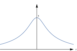
Figure 1. Schematic plot of $c_{\textrm{\tiny ww}}$.

Since $c_{\textrm{\tiny ww}}(\kappa)>c_{\textrm{\tiny ww}}(n\kappa)$ for $n=2,3,\dots$ pointwise in $\mathbb{R}$ (see Figure 1), a straightforward calculation reveals that for any $\kappa>0$, $b_{1}$, $b_{2}\in\mathbb{R}$ and $|b_{1}|$, $|b_{2}|$ sufficiently small, the $H^{1}(\mathbb{T})\times H^{1}(\mathbb{T})$ kernel of $\mathbf{L}_{0}=\partial_{\mathbf{u}}\mathbf{f}(\mathbf{u}_{0},c_{0};\kappa,b_{1},b_{2})$ is two dimensional and spanned by $\mathbf{u}_{1}e^{\pm iz}$ for some nonzero $\mathbf{u}_{1}$ satisfying (2.15). Note from (2.15) and (2.8) that

(2.17) $$\mathbf{u}_{1}=\begin{pmatrix}1+\eta_{0}\\ c_{0}-u_{0}\end{pmatrix}=\begin{pmatrix}1+b_{1}c_{\textrm{\tiny ww}}(\kappa)+b_{2}\\ c_{\textrm{\tiny ww}}(\kappa)+\frac{1}{2}b_{1}c_{\textrm{\tiny ww}}^{2}(\kappa)+\frac{1}{2}b_{2}c_{\textrm{\tiny ww}}(\kappa)\end{pmatrix}+O((b_{1}+b_{2})^{2})$$

as $b_{1}$, $b_{2}\to 0$ up to the multiplication by a constant. This agrees with (2.7a) and (2.7b) at the order of $a$. By the way, in the presence of the effects of surface tension, if $c_{\textrm{\tiny ww}}(\kappa)=c_{\textrm{\tiny ww}}(n\kappa)$ for some integer $n\geqslant 2$ for some $\kappa>0$, resulting in the resonance of the fundamental mode and the $n$-th harmonic, then the kernel would be four dimensional; see Section 5 for details.

Moreover, a straightforward calculation reveals that for any $\kappa>0$, $b_{1}$, $b_{2}\in\mathbb{R}$ and $|b_{1}|$, $|b_{2}|$ sufficiently small, the $H^{1}(\mathbb{T})\times H^{1}(\mathbb{T})$ co-kernel of $\mathbf{L}_{0}$ is two dimensional and spanned by $\mathbf{u}_{1}^{\perp}e^{\pm iz}$ for some $\mathbf{u}_{1}^{\perp}$ orthogonal to $\mathbf{u}_{1}$. In particular, $\mathbf{L}_{0}$ is a Fredholm operator of index zero.

2.6. Lyapunov-Schmidt procedure

For any $\kappa>0$, $b_{1}$, $b_{2}\in\mathbb{R}$ and $|b_{1}|$, $|b_{2}|$ sufficiently small, we turn the attention to non-constant solutions of (2.12)-(2.13) and, hence, (2.3) bifurcating from $\mathbf{u}=\mathbf{u}_{0}$ and $c=c_{0}$, where $\eta_{0}$, $u_{0}$, and $c_{0}$ are in (2.8). A Lyapunov-Schmidt procedure (see [Nir01, Section 2.7.6], for instance) is instrumental for the purpose. Here the proof follows along the same line as the arguments in [HJ15a, HP16], but with suitable modifications to accommodate product spaces. Throughout the subsection, $\kappa$, and $b_{1}$, $b_{2}$ are fixed and suppressed for simplicity of notation.

Recall $\mathbf{f}(\mathbf{u}_{0},c_{0})=\mathbf{0}$, where $\mathbf{f}$ is in (2.12). Recall $\mathbf{L}_{0}\mathbf{u}_{1}e^{\pm iz}=0$, where $\mathbf{L}_{0}$ is in (2.15) and $\mathbf{u}_{1}$ is in (2.17). We write that

(2.18) $$\mathbf{u}(z)=\mathbf{u}_{0}+\frac{1}{2}\mathbf{u}_{1}(ae^{iz}+a^{*}e^{-iz})+\mathbf{u}_{r}(z)\quad\text{and}\quad c=c_{0}+c_{r},$$

and we require that $a\in\mathbb{C}$, $\mathbf{u}_{r}=\begin{pmatrix}\eta_{r}\\ u_{r}\end{pmatrix}\in H^{1}(\mathbb{T})\times H^{1}(\mathbb{T})$ be even and

(2.19) $$\langle\mathbf{u}_{r},\mathbf{u}_{1}(ae^{iz}+a^{*}e^{-iz})\rangle=\frac{1}{2\pi}\int^{\pi}_{-\pi}( (1+\eta_{0})\eta_{r}(z)(ae^{iz}+a^{*}e^{-iz})$$

$$+(c_{0}-u_{0})u_{r}(z)(ae^{iz}+a^{*}e^{-iz}))~{}dz=0,$$

and $c_{r}\in\mathbb{R}$. Here and elsewhere, the asterisk means complex conjugation; $\langle\cdot\,,\cdot\rangle$ is the $L^{2}(\mathbb{T})\times L^{2}(\mathbb{T})$ inner product.

Substituting (2.18) into (2.12)-(2.13), we use $\mathbf{f}(\mathbf{u}_{0};c_{0})=\mathbf{0}$, and (2.15), (2.17), and we make an explicit calculation to arrive at

(2.20) $$\mathbf{L}_{0}\mathbf{u}_{r}= -\begin{pmatrix}\left(\frac{1}{2}(c_{0}-u_{0})(ae^{iz}+a^{*}e^{-iz})+u_{r}\right)\left(\frac{1}{2}(1+\eta_{0})(ae^{iz}+a^{*}e^{-iz})+\eta_{r}\right)\\ \frac{1}{2}\left(\frac{1}{2}(c_{0}-u_{0})(ae^{iz}+a^{*}e^{-iz})+u_{r}\right)^{2}\end{pmatrix}$$

$$+c_{r}\begin{pmatrix}\frac{1}{2}(1+\eta_{0})(ae^{iz}+a^{*}e^{-iz})+\eta_{r}\\ \frac{1}{2}(c_{0}-u_{0})(ae^{iz}+a^{*}e^{-iz})+u_{r}\end{pmatrix}$$

$$=: \mathbf{g}(\mathbf{u}_{r};a,a^{*},c_{r})$$

up to terms of order $c_{r}$ as $c_{r}\to 0$. Recall that $\mathbf{f}$ is a real analytic operator. Hence $\mathbf{g}$ depends analytically on its arguments. Clearly, $\mathbf{g}(\mathbf{0};0,0,c_{r})=0$ for any $c_{r}\in\mathbb{R}$.

Recall that $\mathbf{L}_{0}$ is a Fredholm operator of index zero,

$$\ker\mathbf{L}_{0}=\text{span}\{\mathbf{u}_{1}e^{\pm iz}\}\quad\text{and}\quad\text{co-ker\,}\mathbf{L}_{0}=\text{span}\{\mathbf{u}_{1}^{\perp}e^{\pm iz}\},$$

where $\mathbf{u}_{1}$ and $\mathbf{u}_{1}^{\perp}$ are orthogonal to each other. Let $\Pi$ denote the spectral projection of $L^{2}(\mathbb{T})\times L^{2}(\mathbb{T})$ onto the kernel of $\mathbf{L}_{0}$. Specifically, if $\mathbf{v}={\displaystyle\sum_{n\in\mathbb{Z}}\begin{pmatrix}\widehat{\zeta}(n)\\ \widehat{v}(n)\end{pmatrix}e^{inz}}$ in the Fourier series then

$$\Pi\mathbf{v}= \langle\mathbf{v},\mathbf{u}_{1}e^{iz}\rangle\mathbf{u}_{1}e^{iz}+\langle\mathbf{v},\mathbf{u}_{1}e^{-iz}\rangle\mathbf{u}_{1}e^{-iz}$$

$$= ((1+\eta_{0})(\widehat{\zeta}(1)e^{iz}+\widehat{\zeta}(-1)e^{-iz})+(c_{0}-u_{0})(\widehat{v}(1)e^{iz}+\widehat{v}(-1)e^{-iz}))\mathbf{u}_{1}.$$

Since $\Pi\mathbf{u}_{r}=0$ by (2.19), we may recast (2.20) as

(2.21) $$\mathbf{L}_{0}\mathbf{u}_{r}=(1-\Pi)\mathbf{g}(\mathbf{u}_{r};a,a^{*},c_{r})\quad\text{and}\quad\mathbf{0}=\Pi\mathbf{g}(\mathbf{u}_{r};a,a^{*},c_{r}).$$

Moreover, $\mathbf{L}_{0}:(1-\Pi)(H^{1}(\mathbb{T})\times H^{1}(\mathbb{T}))\to\text{range\,}\mathbf{L}_{0}$ is invertible. Specifically, if

$$\mathbf{v}={\displaystyle\begin{pmatrix}1+\eta_{0}\\ u_{0}-c_{0}\\ \end{pmatrix}(v_{+1}e^{iz}+v_{-1}e^{-iz})+\sum_{n\neq\pm 1}\begin{pmatrix}\widehat{\zeta}(n)\\ \widehat{v}(n)\end{pmatrix}e^{inz}},$$

for some constants $v_{\pm 1}$, belongs to the range of $\mathbf{L}_{0}$ by (2.15) then

$$\mathbf{L}_{0}^{-1}\mathbf{v}(z)= \begin{pmatrix}0\\ 1\end{pmatrix}(v_{+1}e^{iz}+v_{-1}e^{-iz})$$

$$+\sum_{n\neq\pm 1}\frac{1}{(u_{0}-c_{0})^{2}-c_{\textrm{\tiny ww}}^{2}(n\kappa)(1+\eta_{0})}\begin{pmatrix}u_{0}-c_{0}&-1-\eta_{0}\\ -c_{\textrm{\tiny ww}}^{2}(\kappa n)&u_{0}-c_{0}\end{pmatrix}\begin{pmatrix}\widehat{\zeta}(n)\\ \widehat{v}(n)\end{pmatrix}e^{inz}.$$

It is well defined since (2.16) holds true if and only if $n=\pm 1$. Hence we may recast (2.21) as

(2.22) $$\mathbf{u}_{r}=\mathbf{L}_{0}^{-1}(1-\Pi)\mathbf{g}(\mathbf{u}_{r};a,a^{*},c_{r})\quad\text{and}\quad\mathbf{0}=\Pi\mathbf{g}(\mathbf{u}_{r};a,a^{*},c_{r}).$$

Clearly, $\mathbf{L}_{0}^{-1}(1-\Pi)\mathbf{g}$ depends analytically on its arguments. Since $\mathbf{g}(\mathbf{0};0,0,c_{r})=0$ for any $c_{r}\in\mathbb{R}$, it follows from the implicit function theorem that a unique solution $\mathbf{u}_{r}=\mathbf{u}_{2}(a,a^{*},c_{r})$ exists to the former equation of (2.22) near $\mathbf{u}_{r}=\mathbf{0}$ for $a\in\mathbb{C}$ and $|a|$ sufficiently small for any $c_{r}\in\mathbb{R}$. Note that $\mathbf{u}_{2}$ depends analytically on its arguments and it satisfies (2.19) for $|a|$ sufficiently small for any $c_{r}\in\mathbb{R}$. The uniqueness implies

(2.23) $$\mathbf{u}_{2}(0,0,c_{r})=\mathbf{0}\qquad\text{for any $c_{r}\in\mathbb{R}$.}$$

Moreover, since (2.12)-(2.13) and, hence, (2.22) are invariant under (2.6) for any $z_{0}\in\mathbb{R}$, it follows that

(2.24) $$\mathbf{u}_{2}(a,a^{*},c_{r})(z+z_{0})=\mathbf{u}_{2}(ae^{iz_{0}},a^{*}e^{-iz_{0}},c_{r})(z)\quad\text{and}\quad\mathbf{u}_{2}(a,a^{*},c_{r})(-z)=\mathbf{u}_{2}(a,a^{*},c_{r})(z)$$

for any $z_{0}\in\mathbb{R}$ for any $a\in\mathbb{C}$, $|a|$ sufficiently small, and $c_{r}\in\mathbb{R}$.

To proceed, we write the latter equation of (2.22) as

$$\Pi\mathbf{g}(\mathbf{u}_{2}(a,a^{*},c_{r});a,a^{*},c_{r})=\mathbf{0}$$

for $a\in\mathbb{C}$ and $|a|$ sufficiently small for any $c_{r}\in\mathbb{R}$. This is solvable, provided that

(2.25) $$\pi_{\pm}(a,a^{*},c_{r}):=\langle\mathbf{g}(\mathbf{u}_{2}(a,a^{*},c_{r});a,a^{*},c_{r}),\mathbf{u}_{1}(ae^{iz}\pm a^{*}e^{-iz})\rangle=0;$$

$\langle\cdot\,,\cdot\rangle$ is the $L^{2}(\mathbb{T})\times L^{2}(\mathbb{T})$ inner product. We use (2.24), where $z_{0}=-2\arg(a)$, and (2.25) to show that

$$\pi_{-}(a^{*},a,c_{r})=\pi_{-}(a,a^{*},c_{r})=-\pi_{-}(a^{*},a,c_{r}).$$

Hence $\pi_{-}(a,a^{*},c_{r})=0$ holds true for any $a\in\mathbb{C}$ and $|a|$ sufficiently small for any $c_{r}\in\mathbb{R}$. Moreover, we use (2.24), where $z_{0}=-\arg(a)$, and (2.25) to show that

$$\pi_{+}(a,a^{*},c_{r})=\pi_{+}(|a|,|a|,c_{r}).$$

Hence it suffices to solve $\pi_{+}(a,a,c_{r})=0$ for $a$, $c_{r}\in\mathbb{R}$ and $|a|$ sufficiently small.

Substituting (2.20) into (2.25), where $\mathbf{u}_{r}=\mathbf{u}_{2}(a,a,c_{r})=:\begin{pmatrix}\eta_{2}\\ u_{2}\end{pmatrix}(a,c_{r})$, we make an explicit calculation to arrive at

$$\pi_{+}(a,a,c_{r})=:a^{2}(c_{r}((1+\eta_{0})^{2}+(c_{0}-u_{0})^{2})+\pi_{r}(a,c_{r}))$$

for $a$, $c_{r}\in\mathbb{R}$ and $|a|$ sufficiently small, where

$$\pi_{r}(a,c_{r})= -a^{2}(1+\eta_{0})((c_{0}-u_{0})\langle\cos z\,\eta_{2}(a,c_{r}),\cos z\rangle$$

$$\hskip 55.0pt+(1+\eta_{0})\langle\cos z\,u_{2}(a,c_{r}),\cos z\rangle+a^{-1}\langle(\eta_{2}u_{2})(a,c_{r}),\cos z\rangle)$$

$$-\tfrac{1}{2}a^{2}(c_{0}-u_{0})(2(c_{0}-u_{0})\langle\cos z\,u_{2}(a,c_{r}),\cos z\rangle+a^{-1}\langle u_{2}^{2}(a,c_{r}),\cos z\rangle);$$

$\langle\cdot\,,\cdot\rangle$ means the $L^{2}(\mathbb{T})$ inner product. We merely pause to remark that $\pi_{r}$ is well defined. Indeed, $a^{-1}\eta_{2}$ and $a^{-1}u_{2}$ are not singular for $a\in\mathbb{R}$ and $|a|$ sufficiently small by (2.23). Clearly, $\pi_{r}$ and, hence, $\pi_{+}$ depend analytically on their arguments. Since $\pi_{r}(0,0)=0$ and $(\partial_{c_{r}}\pi_{r})(0,0)=0$ by (2.23), it follows from the implicit function theorem that a unique solution $c_{r}=c_{2}(a)$ exists to $\pi_{+}(a,a,c_{r})=0$ and, hence, the latter equation of (2.22) near $c_{r}=0$ for $a\in\mathbb{R}$ and $|a|$ sufficiently small. Clearly, $c_{2}$ depends analytically on $a$.

To summarize,

$$\mathbf{u}_{r}=\mathbf{u}_{2}(a,a,c_{2}(a))\quad\text{and}\quad c_{r}=c_{2}(a)$$

uniquely solve (2.20) for $a\in\mathbb{R}$ and $|a|$ sufficiently small, and by virtue of (2.18),

(2.26) $$\mathbf{u}(a)(z)=\mathbf{u}_{0}+a\mathbf{u}_{1}\cos z+\mathbf{u}_{2}(a,a,c_{2}(a))(z)\quad\text{and}\quad c(a)=c_{0}+c_{2}(a)$$

uniquely solve (2.12)-(2.13) and, hence, (2.3) for $a\in\mathbb{R}$ and $|a|$ sufficiently small. Note that $\mathbf{u}_{2}$ and, hence, $\mathbf{u}$ are $2\pi$ periodic and even in $z$. Since $\mathbf{u}_{2}$ and $c_{2}$ are near $\mathbf{0}$ and $0$, Lemma 2.2 implies that $\mathbf{u}$ is smooth in $z$. We claim that $c$ is even in $a$. Indeed, note that (2.3) and, hence, (2.12)-(2.13) remain invariant under $z\mapsto z+\pi$ by (2.6). Since $(\partial_{a}\mathbf{u})(0)(z)=\mathbf{u}_{1}\cos z$, however, $\mathbf{u}(z)\neq\mathbf{u}(z+\pi)$ must hold true. Thus $(\partial_{a}c)(0)=0$. This proves the claim. Clearly, $\mathbf{u}$ and $c$ depend analytically on $a\in\mathbb{R}$ and $|a|$ sufficiently small. This completes the existence proof.

2.7. Small amplitude expansion

It remains to verify (2.7). Throughout the subsection, $\kappa>0$ is fixed and suppressed for simplicity of notation; $b_{1}$, $b_{2}\in\mathbb{R}$ and $|b_{1}|$, $|b_{2}|$ sufficiently small are fixed.

Recall from the existence proof that (2.26) depends analytically on $a$, $b_{1}$, $b_{2}\in\mathbb{R}$ and $|a|$, $|b_{1}|$, $|b_{2}|$ sufficiently small. We write that

$$\eta(a;b_{1},b_{2})(z)= \eta_{0}(b_{1},b_{2})+a(1+\eta_{0}(b_{1},b_{2}))\cos z$$

$$+a^{2}\eta_{2}(z)+a^{3}\eta_{3}(z)+O(a^{4}+a^{2}(b_{1}+b_{2})+a(b_{1}+b_{2})^{2}),$$

$$u(a;b_{1},b_{2})(z)= u_{0}(b_{1},b_{2})+a(c_{0}-u_{0})(b_{1},b_{2})\cos z$$

$$+a^{2}u_{2}(z)+a^{3}u_{3}(z)+O(a^{4}+a^{2}(b_{1}+b_{2})+a(b_{1}+b_{2})^{2}),$$

and

$$c(a;b_{1},b_{2})= c_{0}(b_{1},b_{2})+a^{2}c_{2}+O(a^{4}+a^{2}(b_{1}+b_{2})+a(b_{1}+b_{2})^{2})$$

as $a,b_{1},b_{2}\to 0$, where $\eta_{0}$, $u_{0}$, and $c_{0}$ are in (2.8), and we require that $\eta_{2}$, $u_{2}$, and $\eta_{3}$, $u_{3}$ be $2\pi$ periodic, even, and smooth functions of $z$, and $c_{2}\in\mathbb{R}$. We merely pause to remark that $\eta_{2}$, $u_{2}$, $\eta_{3}$, $u_{3}$, and $c_{2}$ do not depend on $b_{1}$ and $b_{2}$, whereas $\eta_{0}$, $u_{0}$, and $c_{0}$ do. In the following sections, we restrict the attention to periodic traveling waves of (2.1)-(2.2) for $a\in\mathbb{R}$ and $|a|$ sufficiently small for $b_{1}=b_{2}=0$, and we calculate the spectrum of the associated linearized operator up to the order of $a$. (The index formulae would become unwieldy when terms of order $a^{2}$ were to be added.) For the purpose, it suffices to calculate solutions explicitly up to terms of orders $a^{2}$, and $ab_{1}$, $ab_{2}$.

Substituting the above into (2.3), we recall that $\eta_{0}$, $u_{0}$, and $c_{0}$ solve (2.3), and we make an explicit calculation to arrive, at the order of $a$, at

$$-c_{0}(1+\eta_{0})\cos z+(c_{0}-u_{0})\cos z=0,$$

$$-c_{0}(c_{0}-u_{0})\cos z+c_{\textrm{\tiny ww}}^{2}(\kappa|\partial_{z}|)(1+\eta_{0})\cos z=0.$$

This holds true up to terms of orders $b_{1}$ and $b_{2}$ by (2.2), (2.8c), and (2.15), (2.17).

To proceed, we assume $b_{1}=b_{2}=0$ and, hence, $\eta_{0}=u_{0}=0$ and $c_{0}=c_{\textrm{\tiny ww}}(\kappa)$ by (2.8). At the order of $a^{2}$, we gather

$$-c_{0}\eta_{2}+u_{2}+c_{0}\cos^{2}z=0,$$

$$-c_{0}u_{2}+c_{\textrm{\tiny ww}}^{2}(\kappa|\partial_{z}|)\eta_{2}+\tfrac{1}{2}c_{0}^{2}\cos^{2}z=0.$$

We then use (2.2), (2.8c) and we make an explicit calculation to find

(2.27) $$\eta_{2}(z)=h_{0}+h_{2}\cos 2z\quad\text{and}\quad u_{2}(z)=h_{0}-\frac{1}{2}+\Big{(}h_{2}-\frac{1}{2}\Big{)}\cos 2z,$$

where $h_{0}$ and $h_{2}$ are in (2.9). Continuing, at the order of $a^{3}$, we gather

$$-c_{0}\eta_{3}-c_{2}\cos z+u_{3}+u_{2}\cos z+c_{0}\eta_{2}\cos z=0,$$

$$-c_{0}u_{3}-c_{2}c_{0}\cos z+c_{\textrm{\tiny ww}}^{2}(\kappa|\partial_{z}|)\eta_{3}+c_{0}u_{2}\cos z=0.$$

Taking $L^{2}(\mathbb{T})$ inner products, we use (2.2) and (2.27), so that

$$-c_{0}\langle\eta_{3},\cos z\rangle-c_{2}+\langle u_{3},\cos z\rangle+h_{0}-\frac{1}{2}+\frac{1}{2}\Big{(}h_{2}-\frac{1}{2}\Big{)}+c_{0}\Big{(}h_{0}+\frac{1}{2}h_{2}\Big{)}=0,$$

$$-c_{0}\langle u_{3},\cos z\rangle-c_{2}c_{0}+c_{\textrm{\tiny ww}}^{2}(\kappa)\langle\eta_{3},\cos z\rangle+c_{0}\Big{(}h_{0}-\frac{1}{2}+\frac{1}{2}\Big{(}h_{2}-\frac{1}{2}\Big{)}\Big{)}=0.$$

We then use (2.8c) and we make an explicit calculation to find

$$c_{2}=\frac{3}{4}c_{\textrm{\tiny ww}}(\kappa)(2h_{0}+h_{2}-1).$$

This completes the proof.

3. Modulational instability

Let $\eta=\eta(a;\kappa,b_{1},b_{2})$, $u=u(a;\kappa,b_{1},b_{2})$, and $c=c(a;\kappa,b_{1},b_{2})$, for some $a\in\mathbb{R}$ and $|a|$ sufficiently small, $\kappa>0$, $b_{1}$, $b_{2}\in\mathbb{R}$ and $|b_{1}|$, $|b_{2}|$ sufficiently small, denote a $2\pi/\kappa$-periodic wave train of (2.1)-(2.2), whose existence follows from Theorem 2.1. We address its stability and instability to “slow modulations.” Throughout the section, we employ the notation of (2.11) whenever it is convenient to do so.

Well-posedness

The solution of the linear part of (2.1)-(2.2) does not possess smoothing effects. Hence it is difficult to work out the well-posedness in spaces of low regularities. But, for the present purpose, it suffices to solve the Cauchy problem in some functional analytic setting. In Appendix A, we establish the local-in-time well-posedness for (2.1)-(2.2) in $H^{s}(\mathbb{R})\times H^{s+1/2}(\mathbb{R})$ for any $s>2$.

3.1. Spectral stability and instability

Intuitively, the stability of $\mathbf{u}$ means that if we perturb $\mathbf{u}$ at time $t=0$ then the solution at later times remains near (a spatial translate of) it. In a leading approximation, we will linearize (2.1)-(2.2) about $\mathbf{u}$ in the coordinate frame moving at the speed $c$. Recall that $\mathbf{u}$ and $c$ solve (2.3) and $z=\kappa x$. The result becomes

$$\partial_{t}\mathbf{v}=\kappa\partial_{z}\begin{pmatrix}c-u&-1-\eta\\ -c_{\textrm{\tiny ww}}^{2}(\kappa|\partial_{z}|)&c-u\end{pmatrix}\mathbf{v}.$$

We seek a solution of the form $\mathbf{v}(z,t)=e^{\lambda\kappa t}\mathbf{v}(z)$, $\lambda\in\mathbb{C}$, to arrive at

(3.1) $$\lambda\mathbf{v}=\partial_{z}\begin{pmatrix}c-u&-1-\eta\\ -c_{\textrm{\tiny ww}}^{2}(\kappa|\partial_{z}|)&c-u\end{pmatrix}\mathbf{v}=:\mathcal{L}(a;\kappa,b_{1},b_{2})\mathbf{v},$$

where

$$\mathcal{L}:H^{1}(\mathbb{R})\times H^{1}(\mathbb{R})\subset L^{2}(\mathbb{R})\times L^{2}(\mathbb{R})\to L^{2}(\mathbb{R})\times L^{2}(\mathbb{R}).$$

We say that $\mathbf{u}$ is spectrally unstable to square integrable perturbations if the $L^{2}(\mathbb{R})\times L^{2}(\mathbb{R})$ spectrum of $\mathcal{L}$ intersects the open right-half plane of $\mathbb{C}$, and it is spectrally stable otherwise. Note that $\eta$ and $u$ are $2\pi$ periodic in $z$, but $\mathbf{v}$ needs not.

Note that (3.1) remains invariant under

$$\lambda\mapsto\lambda^{*}\quad\text{and}\quad\mathbf{v}\mapsto\mathbf{v}^{*},$$

where $*$ means complex conjugation, and under

$$\lambda\mapsto-\lambda\quad\text{and}\quad z\mapsto-z.$$

Together, the spectrum of $\mathcal{L}$ is symmetric with respect to the reflections in the real and imaginary axes. Hence $\mathbf{u}$ is spectrally unstable if and only if the spectrum of $\mathcal{L}$ is not contained in the imaginary axis.

Spectral instability reported herein promotes spatially localized and temporally exponentially growing solutions of (2.1)-(2.2). We will investigate this in a future publication. In stark contrast, spectral stability does not in general imply nonlinear stability.

3.2. Floquet characterization of the spectrum

It is well known (see [RS78, Section 8.16] and [Chi06, Section 2.4], for instance, for details; see also [BHJ16]) that the $L^{2}(\mathbb{R})\times L^{2}(\mathbb{R})$ spectrum of $\mathcal{L}$, which by the way involves periodic coefficients, contains no eigenvalues. Rather, it consists of the essential spectrum. Moreover, a nontrivial solution of (3.1) does not belong to $L^{p}(\mathbb{R})\times L^{p}(\mathbb{R})$ for any $p\in[1,\infty)$. Rather, if $\mathbf{v}\in L^{\infty}(\mathbb{R})\times L^{\infty}(\mathbb{R})$ solves (3.1) then, necessarily,

$$\mathbf{v}(z)=e^{i\xi z}\boldsymbol{\phi}(z),\qquad\text{where\quad$\boldsymbol{\phi}(z+2\pi)=\boldsymbol{\phi}(z)$},$$

for some $\xi$ in the range $(-1/2,1/2]$, the Floquet exponent. We take a Floquet theory approach to characterize the $L^{2}(\mathbb{R})\times L^{2}(\mathbb{R})$ spectrum of $\mathcal{L}$ in a convenient form. By the way, $\mathcal{L}$ involves a nonlocal operator. Hence classical Floquet theory is not directly applicable. Details are found in [BHJ16], for instance, and references therein. Hence we merely hit the main points.

We begin by writing $v\in L^{2}(\mathbb{R})$ as

$$v(z)=\frac{1}{\sqrt{2\pi}}\int^{1/2}_{-1/2}\Big{(}\sum_{n\in\mathbb{Z}}\widehat{v}(n+\xi)e^{inz}\Big{)}e^{i\xi z}~{}d\xi=:\int^{1/2}_{-1/2}v(\xi)(z)e^{i\xi z}~{}d\xi,$$

where $\widehat{v}$ means the Fourier transform of $v$. It is well defined in the Schwartz class by the Fubini theorem and the dominated convergence theorem, and it is extended to $L^{2}(\mathbb{R})$ by a density argument. Note that $v(\xi)\in L^{2}(\mathbb{T})$ for any $\xi\in(-1/2,1/2]$. The Parseval theorem asserts that

$$\|v\|_{L^{2}(\mathbb{R})}^{2}=\|\widehat{v}\|_{L^{2}(\mathbb{R})}^{2}=\int^{1/2}_{-1/2}\|v(\xi)\|_{L^{2}(\mathbb{T})}^{2}~{}d\xi.$$

Hence $v\mapsto v(\xi)$ is an isomorphism between $L^{2}(\mathbb{R})$ and $L^{2}((-1/2,1/2];L^{2}(\mathbb{T}))$. Let $\mathcal{M}:L^{2}(\mathbb{R})\to L^{2}(\mathbb{R})$ denote a Fourier multiplier operator, defined as

$$\widehat{\mathcal{M}v}(\kappa)=m(\kappa)\widehat{v}(\kappa)$$

for a suitable function $m$, real valued and Lebesgue measurable. It is straightforward to verity that

$$(\mathcal{M}v)(\xi)=e^{-i\xi z}\mathcal{M}e^{i\xi z}v(\xi)=:\mathcal{M}(\xi)v(\xi)$$

for any $v\in L^{2}(\mathbb{R})$ and $\xi\in(-1/2,1/2]$. Note that $\mathcal{M}(\xi):L^{2}(\mathbb{T})\to L^{2}(\mathbb{T})$ for any $\xi$. Moreover, for a suitable function $f$,

$$(fv)(\xi)=fv(\xi)\qquad\text{for any $v\in L^{2}(\mathbb{R})$ and $\xi\in(-1/2,1/2]$}.$$

We extend this to product spaces in the usual manner. It is then straightforward to verify that

$$(\mathcal{L}\mathbf{v})(\xi)=e^{-i\xi z}\mathcal{L}e^{i\xi z}\mathbf{v}(\xi)=:\mathcal{L}(\xi)\mathbf{v}(\xi)$$

for any $\mathbf{v}\in L^{2}(\mathbb{R})\times L^{2}(\mathbb{R})$ and $\xi\in(-1/2,1/2]$. Note that

$$\mathcal{L}(\xi):H^{1}(\mathbb{T})\times H^{1}(\mathbb{T})\subset L^{2}(\mathbb{T})\times L^{2}(\mathbb{T})\to L^{2}(\mathbb{T})\times L^{2}(\mathbb{T})$$

for any $\xi\in(-1/2,1/2]$.

Furthermore (see [RS78, Section 8.16], for instance, for details; see also [BHJ16]), $\lambda$ belongs to the $L^{2}(\mathbb{R})\times L^{2}(\mathbb{R})$ spectrum of $\mathcal{L}$ if and only if it belongs to the $L^{2}(\mathbb{T})\times L^{2}(\mathbb{T})$ spectrum of $\mathcal{L}(\xi)$ for some $\xi\in(-1/2,1/2]$. That is,

(3.2) $$\lambda\boldsymbol{\phi}=e^{-i\xi z}\partial_{z}\begin{pmatrix}c-u&-1-\eta\\ -c_{\textrm{\tiny ww}}^{2}(\kappa|\partial_{z}|)&c-u\end{pmatrix}e^{i\xi z}\boldsymbol{\phi}$$

for some nontrivial $\boldsymbol{\phi}\in L^{2}(\mathbb{T})\times L^{2}(\mathbb{T})$ and $\xi\in(-1/2,1/2]$. Hence

$$\text{spec}_{L^{2}(\mathbb{R})\times L^{2}(\mathbb{R})}(\mathcal{L})=\bigcup_{\xi\in[-1/2,1/2)}\text{spec}_{L^{2}(\mathbb{T})\times L^{2}(\mathbb{T})}(\mathcal{L}(\xi)).$$

Note that for any $\xi\in(-1/2,1/2]$, the $L^{2}(\mathbb{T})\times L^{2}(\mathbb{T})$ spectrum of $\mathcal{L}(\xi)$ consists of eigenvalues with finite multiplicities. Thus we characterize the essential spectrum of $\mathcal{L}$ as a one parameter family of point spectra of $\mathcal{L}(\xi)$ for $\xi\in(-1/2,1/2]$.

Note that (3.2), when $\pm\xi$ are taken in pair, remains invariant under

$$\lambda\mapsto\lambda^{*}\quad\text{and}\quad\boldsymbol{\phi}\mapsto\boldsymbol{\phi}^{*},$$

and under

$$\lambda\mapsto-\lambda\quad\text{and}\quad z\mapsto-z.$$

Hence we may assume $\xi\in[0,1/2]$.

3.3. Definition of modulational instability

Note that $\xi=0$ corresponds to the same period perturbations as $\mathbf{u}$. Moreover, $\xi>0$ and small corresponds to long wavelength perturbations, whose effects are to slowly vary the period and other wave characteristics, such as the amplitude. They supply the spectral information of $\mathcal{L}$ in the vicinity of the origin in $\mathbb{C}$; see [BHJ16], for instance, for details. We then say that $\mathbf{u}$ is modulationally unstable if the $L^{2}(\mathbb{T})\times L^{2}(\mathbb{T})$ spectra of $\mathcal{L}(\xi)$ are not contained in the imaginary axis near the origin for $\xi>0$ and small, and it is modulationally stable otherwise.

For an arbitrary $\xi$, one must study (3.2) numerically except for few cases — for instance, completely integrable systems (see [BHJ16], for instance, for references). But, for $\xi>0$ and small for $\lambda$ in the vicinity of the origin in $\mathbb{C}$, we may take a spectral perturbation approach in [HJ15a, HP16], for instance, to address it analytically. This is the subject of investigation here.

Notation

In the remaining of the section, $\kappa>0$ is suppressed for simplicity of notation, unless specified otherwise. We assume $b_{1}=b_{2}=0$. For nonzero $b_{1}$ and $b_{2}$, one may explore in like manner. But the calculation becomes lengthy and tedious. Hence we do not discuss the details. We use

(3.3) $$\mathcal{L}(\xi,a)=\mathcal{L}(\xi)(a;\kappa,0,0)$$

for simplicity of notation.

3.4. Spectra of $\mathcal{L}(\xi,0)$

We begin by discussing the $L^{2}(\mathbb{T})\times L^{2}(\mathbb{T})$ spectra of $\mathcal{L}(\xi,0)$ for $\xi\in[0,1/2]$. This is the linearization of (2.1)-(2.2) about $\eta=u=0$ and $c=c_{\textrm{\tiny ww}}(\kappa)$ — namely, the rest state — in the moving coordinate frame.

Note from (3.2) and (2.8) that

$$\mathcal{L}(\xi,0)=e^{-i\xi z}\partial_{z}\begin{pmatrix}c_{\textrm{\tiny ww}}(\kappa)&-1\\ -c_{\textrm{\tiny ww}}^{2}(\kappa|\partial_{z}|)&c_{\textrm{\tiny ww}}(\kappa)\end{pmatrix}e^{i\xi z}.$$

We use (2.5) and make an explicit calculation to show that

(3.4) $$\mathcal{L}(\xi,0)\mathbf{e}(n+\xi,\pm)=i\omega(n+\xi,\pm)\mathbf{e}(n+\xi,\pm)\qquad\text{for $n\in\mathbb{Z}$ and $\xi\in[0,1/2]$,}$$

where

(3.5) $$\omega(n+\xi,\pm)=(n+\xi)(c_{\textrm{\tiny ww}}(\kappa)\pm c_{\textrm{\tiny ww}}(\kappa(n+\xi)))\quad\text{and}\quad\mathbf{e}(n+\xi,\pm)(z)=\begin{pmatrix}1\\ \mp c_{\textrm{\tiny ww}}(\kappa(n+\xi))\end{pmatrix}e^{inz}.$$

Hence for any $\xi\in[0,1/2]$, the spectrum of $\mathcal{L}(\xi,0)$ consists of two families of infinitely many and purely imaginary eigenvalues, each with finite multiplicity. In particular, the rest state of (2.1)-(2.2) is spectrally stable to square integrable perturbations.

The spectrum of the linear operator associated with the water wave problem consists of $i\omega(n+\xi,\pm)$ for $n\in\mathbb{Z}$ and $\xi\in[-1/2,1/2)$; see [Whi74], for instance, for details. To compare, the spectrum of the linear operator for the Whitham equation (see (1.3)) consists of $i\omega(n+\xi,-)$ for $n\in\mathbb{Z}$ and $\xi\in[-1/2,1/2)$; see [HJ15a], for instance, for details. Perhaps, this is because the Whitham equation merely includes unidirectional propagation. In the following section, we discuss the effects of bidirectional propagation in (2.1)-(2.2).

As $|a|$ increases, the eigenvalues in (3.4) move around and they may leave the imaginary axis to lose the spectral stability. Recall that the spectrum of $\mathcal{L}(\pm\xi,a)$ is symmetric with respect to the reflections in the real and imaginary axes for any $\xi\in[0,1/2]$ for any $a\in\mathbb{R}$ and admissible. Hence a necessary condition of the spectral instability is that a pair of eigenvalues on the imaginary axis collide.

Note that the eigenfunctions in (3.4) vary, analytically, with $\xi\in[0,1/2]$. To compare, the eigenfunctions of the linear operator for the Whitham equation do not depend on $\xi$; see [HJ15a], for instance, for details.

To proceed, for $\xi=0$, note from (3.5) that

$$\omega(0,+)=\omega(0,-)=\omega(1,-)=\omega(-1,-)=0.$$

Since

$$\cdots<\omega(-3,-)<\omega(-2,-)< 0<\omega(2,-)<\omega(3,-)<\cdots$$

and

$$\cdots<\omega(-2,+)<\omega(-1,+)< 0<\omega(1,+)<\omega(2,+)<\dots$$

by brutal force, zero is an $L^{2}(\mathbb{T})\times L^{2}(\mathbb{T})$ eigenvalue of $\mathcal{L}(0,0)$ with multiplicity four. Note that

(3.6) $$\boldsymbol{\phi}_{1}(z):=\frac{1}{2}(\mathbf{e}(1,-)+\mathbf{e}(-1,-))(z)=\begin{pmatrix}1\\ c_{\textrm{\tiny ww}}(\kappa)\end{pmatrix}\cos z,$$

$$\boldsymbol{\phi}_{2}(z):=\frac{1}{2i}(\mathbf{e}(1,-)-\mathbf{e}(-1,-))(z)=\begin{pmatrix}1\\ c_{\textrm{\tiny ww}}(\kappa)\end{pmatrix}\sin z,$$

$$\boldsymbol{\phi}_{3}(z):=\frac{1}{2}((c_{\textrm{\tiny ww}}(\kappa)+2)\mathbf{e}(0,+)-(c_{\textrm{\tiny ww}}(\kappa)-2)\mathbf{e}(0,-))(z)=\begin{pmatrix}2\\ -c_{\textrm{\tiny ww}}(\kappa)\end{pmatrix},$$

$$\boldsymbol{\phi}_{4}(z):=\frac{1}{2}((c_{\textrm{\tiny ww}}(\kappa)-2)\mathbf{e}(0,+)+(c_{\textrm{\tiny ww}}(\kappa)+2)\mathbf{e}(0,-))(z)=\begin{pmatrix}c_{\textrm{\tiny ww}}(\kappa)\\ 2\end{pmatrix}$$

are the associated eigenfunctions, real valued and orthogonal to each other.

For $\xi\neq 0$, since $\omega(n+\xi,+)$ increases in $n+\xi$ for any $n\in\mathbb{Z}$ and $\xi\in(0,1/2]$, and since $\omega(n+\xi,-)$ decreases in $n+\xi$ if $-1/2<n+\xi<1/2$ and increases if $n+\xi<-1$ or $n+\xi>1$ by brutal force, it follows that

$$\omega(1/2,-)\leqslant\omega(0+\xi,\pm),\omega(\pm 1+\xi,-)\leqslant\omega(1/2,+),$$

and

$$\cdots<\omega(-2+\xi,-)<\omega(\xi,-)<0<\omega(-1+\xi,-)<\omega(1+\xi,-)<\omega(2+\xi,-)<\cdots,$$

$$\cdots<\omega(-2+\xi,+)<\omega(-1+\xi,+)<0<\omega(\xi,+)<\omega(1+\xi,+)<\omega(2+\xi,+)<\cdots.$$

Hence $\omega(n+\xi,\pm)\neq 0$ for any $n\in\mathbb{Z}$ and $\xi\in(0,1/2]$. But in Section 4.1, we observe infinitely many collisions of purely imaginary eigenvalues of $\mathcal{L}(\xi,0)$ away from the origin. To compare, no eigenvalues of the linear operator for the Whitham equation (see (1.3)) collide other than at the origin; see [HJ15a], for instance.

Continuing, for $\xi>0$ and sufficiently small, $i\omega(\xi,\pm)$ and $i\omega(\pm 1+\xi,-)$ are $L^{2}(\mathbb{T})\times L^{2}(\mathbb{T})$ eigenvalues of $\mathcal{L}(\xi,0)$ in the vicinity of the origin in $\mathbb{C}$. Moreover, (by abuse of notation)

(3.7) $$\boldsymbol{\phi}_{1}(z):= \frac{1}{2}\sqrt{c_{\textrm{\tiny ww}}^{2}(\kappa)+1}\left(\frac{\mathbf{e}(1+\xi,-)}{\|\mathbf{e}(1+\xi,-)\|}+\frac{\mathbf{e}(-1+\xi,-)}{\|\mathbf{e}(-1+\xi,-)\|}\right)(z)$$

$$= \begin{pmatrix}1\\ c_{\textrm{\tiny ww}}(\kappa)\end{pmatrix}\cos z+i\xi\frac{\kappa c_{\textrm{\tiny ww}}^{\prime}(\kappa)}{c_{\textrm{\tiny ww}}^{2}(\kappa)+1}\begin{pmatrix}-c_{\textrm{\tiny ww}}(\kappa)\\ 1\end{pmatrix}\sin z+\xi^{2}\mathbf{p}_{2}\cos z+O(\xi^{3}),$$

$$\boldsymbol{\phi}_{2}(z):= \frac{1}{2i}\sqrt{c_{\textrm{\tiny ww}}^{2}(\kappa)+1}\left(\frac{\mathbf{e}(1+\xi,-)}{\|\mathbf{e}(1+\xi,-)\|}-\frac{\mathbf{e}(-1+\xi,-)}{\|\mathbf{e}(-1+\xi,-)\|}\right)(z)$$

$$= \begin{pmatrix}1\\ c_{\textrm{\tiny ww}}(\kappa)\end{pmatrix}\sin z-i\xi\frac{\kappa c_{\textrm{\tiny ww}}^{\prime}(\kappa)}{c_{\textrm{\tiny ww}}^{2}(\kappa)+1}\begin{pmatrix}-c_{\textrm{\tiny ww}}(\kappa)\\ 1\end{pmatrix}\cos z+\xi^{2}\mathbf{p}_{2}\sin z+O(\xi^{3}),$$

$$\boldsymbol{\phi}_{3}(z):= \frac{1}{2}((c_{\textrm{\tiny ww}}(\kappa)+2)\mathbf{e}(\xi,+)-(c_{\textrm{\tiny ww}}(\kappa)-2)\mathbf{e}(\xi,-))(z)$$

$$= \begin{pmatrix}2\\ -c_{\textrm{\tiny ww}}(\kappa)\end{pmatrix}+\frac{1}{6}\xi^{2}\kappa^{2}c_{\textrm{\tiny ww}}(\kappa)\begin{pmatrix}0\\ 1\end{pmatrix}+O(\xi^{3}),$$

$$\boldsymbol{\phi}_{4}(z):= \frac{1}{2}((c_{\textrm{\tiny ww}}(\kappa)-2)\mathbf{e}(\xi,+)+(c_{\textrm{\tiny ww}}(\kappa)+2)\mathbf{e}(\xi,-))(z)$$

$$= \begin{pmatrix}c_{\textrm{\tiny ww}}(\kappa)\\ 2\end{pmatrix}-\frac{1}{3}\xi^{2}\kappa^{2}\begin{pmatrix}0\\ 1\end{pmatrix}+O(\xi^{3})$$

span the associated eigenspace, orthogonal to each other, where $\|\cdot\|=\sqrt{\langle\cdot\,,\cdot\rangle_{L^{2}(\mathbb{T})\times L^{2}(\mathbb{T})}}$ and

(3.8) $$\mathbf{p}_{2}=\frac{1}{2}\frac{\kappa^{2}}{c_{\textrm{\tiny ww}}^{2}(\kappa)+1}\begin{pmatrix}{\displaystyle c_{\textrm{\tiny ww}}^{\prime}(\kappa)^{2}\frac{2c_{\textrm{\tiny ww}}^{2}(\kappa)-1}{c_{\textrm{\tiny ww}}^{2}(\kappa)+1}-(c_{\textrm{\tiny ww}}c_{\textrm{\tiny ww}}^{\prime\prime})(\kappa)}\\ {\displaystyle-3\frac{(c_{\textrm{\tiny ww}}(c_{\textrm{\tiny ww}}^{\prime})^{2})(\kappa)}{c_{\textrm{\tiny ww}}^{2}(\kappa)+1}+c_{\textrm{\tiny ww}}^{\prime\prime}(\kappa)}\end{pmatrix}.$$

Here and elsewhere, the prime means ordinary differentiation. For $\xi=0$, note that $\boldsymbol{\phi}_{1}$, $\boldsymbol{\phi}_{2}$, $\boldsymbol{\phi}_{3}$, $\boldsymbol{\phi}_{4}$ become (3.6). Recall that $c_{\textrm{\tiny ww}}$ is a real analytic function. Hence they depend analytically on $\xi\in[0,1/2]$.

Note that $\boldsymbol{\phi}_{1}$ and $\boldsymbol{\phi}_{2}$ vary with $\xi>0$ and sufficiently small to the linear order. In the following subsection, we take this into account and construct an eigenspace for $\xi$, $a\neq 0$ and sufficiently small, which varies analytically with $\xi$ and $a$; see (3.10) for details. Consequently, the spectral perturbation calculation in Section 3.6 becomes lengthy and complicated. To compare, the eigenfunctions of the linear operator for the Whitham equation (see (1.3)) do not depend on $\xi$ for any $a\in\mathbb{R}$ and admissible; see [HJ15a], for instance, for details.

Note that $\boldsymbol{\phi}_{1}$ and $\boldsymbol{\phi}_{2}$ are complex valued. For real valued functions, one must take $\pm\xi$ in pair and deal with six functions. But the spectral perturbation calculation in Section 3.6 involves complex valued operators anyway. Hence this is not worth the effort.

3.5. Spectra of $\mathcal{L}(\xi,a)$

We turn the attention to the $L^{2}(\mathbb{T})\times L^{2}(\mathbb{T})$ spectra of $\mathcal{L}(\xi,a)$ in the vicinity of the origin in $\mathbb{C}$, for $\xi\in[0,1/2]$ for $a\in\mathbb{R}$ and $|a|$ sufficiently small.

Note from (3.2) and (2.7) that

$$\mathcal{L}(\xi,a)= e^{-i\xi z}\partial_{z}\begin{pmatrix}c-u&-1-\eta\\ -c_{\textrm{\tiny ww}}^{2}(\kappa|\partial_{z}|)&c-u\end{pmatrix}e^{i\xi z}$$

$$= e^{-i\xi z}\partial_{z}\left(\begin{pmatrix}c_{\textrm{\tiny ww}}(\kappa)&-1\\ -c_{\textrm{\tiny ww}}^{2}(\kappa|\partial_{z}|)&c_{\textrm{\tiny ww}}(\kappa)\end{pmatrix}+a\begin{pmatrix}-c_{\textrm{\tiny ww}}(\kappa)&-1\\ 0&-c_{\textrm{\tiny ww}}(\kappa)\end{pmatrix}\cos z\right)e^{i\xi z}+O(a^{2})$$

as $a\to 0$, whence

$$\|\mathcal{L}(\xi,a)-\mathcal{L}(\xi,0)\|_{L^{2}(\mathbb{T})\times L^{2}(\mathbb{T})\to L^{2}(\mathbb{T})\times L^{2}(\mathbb{T})}=O(a)$$

as $a\to 0$ uniformly for $\xi\in[0,1/2]$. Recall from the previous subsection that the $L^{2}(\mathbb{T})\times L^{2}(\mathbb{T})$ spectrum of $\mathcal{L}(\xi,0)$ contains four purely imaginary eigenvalues $i\omega(\xi,\pm)$, $i\omega(\pm 1+\xi,-)$ in the vicinity of the origin in $\mathbb{C}$ for $\xi>0$ and sufficiently small. Since $\mathcal{L}(\xi,a)$ depends analytically on $\xi\in[0,1/2]$ and $a\in\mathbb{R}$ admissible, it follows from perturbation theory (see [Kat76, Section 4.3.1], for instance, for details) that the $L^{2}(\mathbb{T})\times L^{2}(\mathbb{T})$ spectrum of $\mathcal{L}(\xi,a)$ contains four eigenvalues, denoted

$$\lambda_{1}(\xi,a),\lambda_{2}(\xi,a),\lambda_{3}(\xi,a),\lambda_{4}(\xi,a),$$

near the origin for $\xi>0$, $a\in\mathbb{R}$ and $\xi$, $|a|$ sufficiently small.

Moreover, a straightforward calculation reveals that

$$|\lambda_{k}(\xi,0)-\lambda_{\ell}(\xi,0)|\geqslant\omega_{0}>0\qquad\text{for $k,\ell=1,2,3,4$ and $k\neq\ell$}$$

for any $\xi\geqslant\xi_{0}>0$ for any $\xi_{0}$ for some $\omega_{0}$. Hence it follows from perturbation theory that $\lambda_{1}$, $\lambda_{2}$, $\lambda_{3}$, $\lambda_{4}$ remain purely imaginary for any $\xi\geqslant\xi_{0}>0$ for any $\xi_{0}$, for any $a\in\mathbb{R}$ and $|a|$ sufficiently small. In particular, a sufficiently small, periodic wave train of (2.1)-(2.2) is spectrally stable to “short wavelength perturbations” in the vicinity of the origin in $\mathbb{C}$. For $\xi=0$, on the other hand, we demonstrate that four eigenvalues collide at the origin.

Lemma 3.1 (Spectrum of $\mathcal{L}(0,a)$).

For $a\in\mathbb{R}$ and $|a|$ sufficiently small, zero is an $L^{2}(\mathbb{T})\times L^{2}(\mathbb{T})$ eigenvalue of $\mathcal{L}(0,a)$ with algebraic multiplicity four and geometric multiplicity three. Moreover, (by abuse of notation)

(3.9a) $$\boldsymbol{\phi}_{1}(z):= \frac{2}{c_{\emph{\tiny ww}}^{2}(\kappa)+2}((\partial_{b_{1}}c)(\partial_{a}\mathbf{u})-(\partial_{a}c)(\partial_{b_{1}}\mathbf{u}))(z)$$

$$= \begin{pmatrix}1\\ c_{\emph{\tiny ww}}(\kappa)\end{pmatrix}\cos z+a\begin{pmatrix}-3h_{2}\dfrac{c_{\emph{\tiny ww}}^{2}(\kappa)}{c_{\emph{\tiny ww}}^{2}(\kappa)+2}\\ c_{\emph{\tiny ww}}(\kappa)\Big{(}\frac{1}{2}-3h_{2}\dfrac{1}{c_{\emph{\tiny ww}}^{2}(\kappa)+2}\Big{)}\end{pmatrix}$$

$$\hskip 68.0pt+2a\begin{pmatrix}h_{2}\\ c_{\emph{\tiny ww}}(\kappa)\left(h_{2}-\frac{1}{2}\right)\end{pmatrix}\cos 2z+O(a^{2}),$$

(3.9b) $$\boldsymbol{\phi}_{2}(z):= -\frac{1}{a}(\partial_{z}\mathbf{u})(z)$$

$$= \begin{pmatrix}1\\ c_{\emph{\tiny ww}}(\kappa)\end{pmatrix}\sin z+2a\begin{pmatrix}h_{2}\\ c_{\emph{\tiny ww}}(\kappa)\left(h_{2}-\frac{1}{2}\right)\end{pmatrix}\sin 2z+O(a^{2}),$$

where $$h_{2}$$ is in (2.9), and

(3.9c) $$\boldsymbol{\phi}_{3}(z):= \frac{2}{c_{\emph{\tiny ww}}^{2}(\kappa)-1}((\partial_{b_{1}}c)(\partial_{b_{2}}\mathbf{u})-(\partial_{b_{2}}c)(\partial_{b_{1}}\mathbf{u}))(z)$$

$$= \begin{pmatrix}2\\ -c_{\emph{\tiny ww}}(\kappa)\end{pmatrix}+a\begin{pmatrix}2\\ c_{\emph{\tiny ww}}(\kappa)\end{pmatrix}\cos z+O(a^{2}),$$

(3.9d) $$\boldsymbol{\phi}_{4}(z):= \frac{1}{3}\frac{c_{\emph{\tiny ww}}^{2}(\kappa)+4}{c_{\emph{\tiny ww}}(\kappa)}\Big{(}(\partial_{b_{2}}\mathbf{u})+\frac{c_{\emph{\tiny ww}}^{2}(\kappa)-2}{c_{\emph{\tiny ww}}^{2}(\kappa)+4}\boldsymbol{\phi}_{3,a}\Big{)}(z)$$

$$= \begin{pmatrix}c_{\emph{\tiny ww}}(\kappa)\\ 2\end{pmatrix}+a\begin{pmatrix}c_{\emph{\tiny ww}}(\kappa)\\ \frac{1}{2}c_{\emph{\tiny ww}}^{2}(\kappa)\end{pmatrix}\cos z+O(a^{2}),$$

are the associated eigenfunctions. Specifically,

$$\mathcal{L}(0,a)\boldsymbol{\phi}_{k}=0\quad\text{for $k=1,2,3,$}\quad\text{and}\quad\mathcal{L}(0,a)\boldsymbol{\phi}_{4}=\frac{1}{4}a(c_{\emph{\tiny ww}}^{2}(\kappa)+1)\boldsymbol{\phi}_{2}.$$

For $a=0$, note that $\boldsymbol{\phi}_{1}$, $\boldsymbol{\phi}_{2}$, $\boldsymbol{\phi}_{3}$, $\boldsymbol{\phi}_{4}$ becomes (3.6). Theorem 2.1 implies that they depend analytically on $a\in\mathbb{R}$ and $|a|$ sufficiently small.

Proof.

Exploiting variations of (2.3) in the $z$, and $a$, $b_{1}$, $b_{2}$ variables, the proof is similar to that of [HJ15a, Lemma 3.1], for instance. Here we include the details for the sake of completeness.

Differentiating (2.3) with respect to $z$ and evaluating the result at $b_{1}=b_{2}=0$, we infer from (3.1) that

$$\mathcal{L}(0,a)(\partial_{z}\mathbf{u})=0.$$

Hence zero is an eigenvalue of $\mathcal{L}(0,a)$ and $\partial_{z}\mathbf{u}$ is an associated eigenfunction. We then use (2.7a) and (2.7b) to find (3.9b). By the way, this is reminiscent of that (2.3) remains invariant under spatial translations.

Differentiating (2.3) with respect to $a$, and $b_{1}$, $b_{2}$, and evaluating at $b_{1}=b_{2}=0$, we infer from (3.1) that

$$\mathcal{L}(0,a)(\partial_{a}\mathbf{u})=-(\partial_{a}c)(\partial_{z}\mathbf{u}),$$

and

$$\mathcal{L}(0,a)(\partial_{b_{1}}\mathbf{u})=-(\partial_{b_{1}}c)(\partial_{z}\mathbf{u}),\qquad\mathcal{L}(0,a)(\partial_{b_{2}}\mathbf{u})=-(\partial_{b_{2}}c)(\partial_{z}\mathbf{u}).$$

Hence

$$\mathcal{L}(0,a)((\partial_{b_{1}}c)(\partial_{a}\mathbf{u})-(\partial_{a}c)(\partial_{b_{1}}\mathbf{u}))=0\quad\text{and}\quad\mathcal{L}(0,a)((\partial_{b_{1}}c)(\partial_{b_{2}}\mathbf{u})-(\partial_{b_{2}}c)(\partial_{b_{1}}\mathbf{u}))=0.$$

We then use (2.7) and (2.8) to find (3.9a) and (3.9c). Note that $\partial_{b_{2}}\mathbf{u}$ is a generalized eigenfunction. We use (2.7) and (2.8) to find (3.9d). This completes the proof. ∎

To recapitulate, for $\xi>0$ and sufficiently small for $a=0$, the $L^{2}(\mathbb{T})\times L^{2}(\mathbb{T})$ spectrum of $\mathcal{L}(\xi,0)$ contains four purely imaginary eigenvalues $i\omega(\xi,\pm)$, $i\omega(\pm 1+\xi,-)$ in the vicinity of the origin in $\mathbb{C}$, and (3.7) spans the associated eigenspace, which depends analytically on $\xi$. For $\xi=0$ for $a\in\mathbb{R}$ and $|a|$ sufficiently small, the spectrum of $\mathcal{L}(0,a)$ contains four eigenvalues at the origin, and (3.9) makes the associated eigenfunctions, which depends analytically on $a$.

For $\xi>0$, $a\in\mathbb{R}$ and $\xi$, $|a|$ sufficiently small, the $L^{2}(\mathbb{T})\times L^{2}(\mathbb{T})$ spectrum of $\mathcal{L}(\xi,a)$ contains four eigenvalues $\lambda_{1}(\xi,a)$, $\lambda_{2}(\xi,a)$, $\lambda_{3}(\xi,a)$, $\lambda_{4}(\xi,a)$ near the origin, and the associated eigenfunctions vary analytically from (3.7) and (3.9). Let (by abuse of notation)

(3.10) $$\boldsymbol{\phi}_{1}(\xi,a)(z)= \begin{pmatrix}1\\ c_{\textrm{\tiny ww}}(\kappa)\end{pmatrix}\cos z+i\xi\frac{\kappa c_{\textrm{\tiny ww}}^{\prime}(\kappa)}{c_{\textrm{\tiny ww}}^{2}(\kappa)+1}\begin{pmatrix}-c_{\textrm{\tiny ww}}(\kappa)\\ 1\end{pmatrix}\sin z$$

$$+a\begin{pmatrix}-3h_{2}\dfrac{c_{\textrm{\tiny ww}}^{2}(\kappa)}{c_{\textrm{\tiny ww}}^{2}(\kappa)+2}\\ c_{\textrm{\tiny ww}}(\kappa)\Big{(}\frac{1}{2}-3h_{2}\dfrac{1}{c_{\textrm{\tiny ww}}^{2}(\kappa)+2}\Big{)}\end{pmatrix}+2a\begin{pmatrix}h_{2}\\ c_{\textrm{\tiny ww}}(\kappa)\left(h_{2}-\frac{1}{2}\right)\end{pmatrix}\cos 2z$$

$$+\xi^{2}\mathbf{p}_{2}\cos z+O(\xi^{3}+\xi^{2}a+a^{2}),$$

$$\boldsymbol{\phi}_{2}(\xi,a)(z)= \begin{pmatrix}1\\ c_{\textrm{\tiny ww}}(\kappa)\end{pmatrix}\sin z-i\xi\frac{\kappa c_{\textrm{\tiny ww}}^{\prime}(\kappa)}{c_{\textrm{\tiny ww}}^{2}(\kappa)+1}\begin{pmatrix}-c_{\textrm{\tiny ww}}(\kappa)\\ 1\end{pmatrix}\cos z$$

$$+2a\begin{pmatrix}h_{2}\\ c_{\textrm{\tiny ww}}(\kappa)\left(h_{2}-\frac{1}{2}\right)\end{pmatrix}\sin 2z+\xi^{2}\mathbf{p}_{2}\sin z+O(\xi^{3}+\xi^{2}a+a^{2}),$$

$$\boldsymbol{\phi}_{3}(\xi,a)(z)= \begin{pmatrix}2\\ -c_{\textrm{\tiny ww}}(\kappa)\end{pmatrix}+a\begin{pmatrix}2\\ c_{\textrm{\tiny ww}}(\kappa)\end{pmatrix}\cos z+\frac{1}{6}\xi^{2}\kappa^{2}c_{\textrm{\tiny ww}}(\kappa)\begin{pmatrix}0\\ 1\end{pmatrix}+O(\xi^{3}+\xi^{2}a+a^{2}),$$

$$\boldsymbol{\phi}_{4}(\xi,a)(z)= \begin{pmatrix}c_{\textrm{\tiny ww}}(\kappa)\\ 2\end{pmatrix}+a\begin{pmatrix}c_{\textrm{\tiny ww}}(\kappa)\\ \frac{1}{2}c_{\textrm{\tiny ww}}^{2}(\kappa)\end{pmatrix}\cos z-\frac{1}{3}\xi^{2}\kappa^{2}\begin{pmatrix}0\\ 1\end{pmatrix}+O(\xi^{3}+\xi^{2}a+a^{2})$$

as $\xi$, $a\to 0$, where $h_{2}$ is in (2.9) and $\mathbf{p}_{2}$ is in (3.9b). For $a=0$, note that $\boldsymbol{\phi}_{1}$, $\boldsymbol{\phi}_{2}$, $\boldsymbol{\phi}_{3}$, $\boldsymbol{\phi}_{4}$ become (3.7). For $\xi=0$, they become (3.9). Hence $\boldsymbol{\phi}_{1}$, $\boldsymbol{\phi}_{2}$, $\boldsymbol{\phi}_{3}$, $\boldsymbol{\phi}_{4}$ span the eigenspace associated with $\lambda_{1}$, $\lambda_{2}$, $\lambda_{3}$, $\lambda_{4}$ up to terms of orders $\xi^{2}$ and $a$ as $\xi$, $a\to 0$.

It seems impossible to uniquely determine terms of orders $\xi a$ and higher in the eigenfunction expansion without ad hoc orthogonality conditions. Fortuitously, it turns out that they do not contribute to the modulational instability. Hence we may neglect them in (3.10). To compare, the eigenfunctions of the linear operator for the Whitham equation (see (1.3)), which do not depend on $\xi$, extend to $a\neq 0$; see [HJ15a], for instance, for details. We are able to calculate terms of orders $a^{2}$ and higher in the eigenfunction expansion. But the index formulae become unwieldy. Hence we do not use them in the calculation in the following subsection.

3.6. Spectral perturbation calculation

Recall that for $\xi>0$, $a\in\mathbb{R}$ and $\xi$, $|a|$ sufficiently small, the $L^{2}(\mathbb{T})\times L^{2}(\mathbb{T})$ spectrum of $\mathcal{L}(\xi,a)$ contains four eigenvalues $\lambda_{1}(\xi,a)$, $\lambda_{2}(\xi,a)$, $\lambda_{3}(\xi,a)$, $\lambda_{4}(\xi,a)$ in the vicinity of the origin in $\mathbb{C}$, and (3.10) spans the associated eigenspace up to terms of orders $\xi^{2}$ and $a$. Let

(3.11) $$\mathbf{L}(\xi,a)=\left(\frac{\langle\mathcal{L}(\xi,a)\boldsymbol{\phi}_{k}(\xi,a),\boldsymbol{\phi}_{\ell}(\xi,a)\rangle}{\langle\boldsymbol{\phi}_{k}(\xi,a),\boldsymbol{\phi}_{k}(\xi,a)\rangle}\right)_{k,\ell=1,2,3,4}$$

and

(3.12) $$\mathbf{I}(\xi,a)=\left(\frac{\langle\boldsymbol{\phi}_{k}(\xi,a),\boldsymbol{\phi}_{\ell}(\xi,a)\rangle}{\langle\boldsymbol{\phi}_{k}(\xi,a),\boldsymbol{\phi}_{k}(\xi,a)\rangle}\right)_{k,\ell=1,2,3,4},$$

where $\boldsymbol{\phi}_{1}$, $\boldsymbol{\phi}_{2}$, $\boldsymbol{\phi}_{3}$, $\boldsymbol{\phi}_{4}$ are in (3.10). Throughout the subsection, $\langle\,,\rangle$ means the $L^{2}(\mathbb{T})\times L^{2}(\mathbb{T})$ inner product. Note that $\mathbf{L}$ represents the action of $\mathcal{L}(\xi,a)$ on the eigenspace associated with $\lambda_{1}$, $\lambda_{2}$, $\lambda_{3}$, $\lambda_{4}$, up to the orders of $\xi^{2}$ and $a$ as $\xi$, $a\to 0$, after normalization, and $\mathbf{I}$ is the projection of the identity onto the eigenspace. It follows from perturbation theory (see [Kat76, Section 4.3.5], for instance, for details) that for $\xi>0$, $a\in\mathbb{R}$ and $\xi$, $|a|$ sufficiently small, the roots of $\det(\mathbf{L}-\lambda\mathbf{I})$ coincide with the eigenvalues of $\mathcal{L}(\xi,a)$ up to terms of orders $\xi^{2}$ and $a$.

For any $a\in\mathbb{R}$ and $|a|$ sufficiently small, we make a Baker-Campbell-Hausdorff expansion to write

$$\mathcal{L}(\xi,a)=\mathcal{L}_{0}+i\xi\mathcal{L}_{1}-\frac{1}{2}\xi^{2}\mathcal{L}_{2}+O(\xi^{3})$$

as $\xi\to 0$, where

$$\mathcal{L}_{0}= \mathcal{L}(0,a)=\partial_{z}\begin{pmatrix}c_{\textrm{\tiny ww}}(\kappa)&-1\\ -c_{\textrm{\tiny ww}}^{2}(\kappa|\partial_{z}|)&c_{\textrm{\tiny ww}}(\kappa)\end{pmatrix}-a\partial_{z}\begin{pmatrix}c_{\textrm{\tiny ww}}(\kappa)&1\\ 0&c_{\textrm{\tiny ww}}(\kappa)\end{pmatrix}\cos z+O(a^{2}),$$

$$\mathcal{L}_{1}= [\mathcal{L}_{0},z]=\begin{pmatrix}c_{\textrm{\tiny ww}}(\kappa)&-1\\ -[\partial_{z}c_{\textrm{\tiny ww}}^{2}(\kappa|\partial_{z}|),z]&c_{\textrm{\tiny ww}}(\kappa)\end{pmatrix}-a\begin{pmatrix}c_{\textrm{\tiny ww}}(\kappa)&1\\ 0&c_{\textrm{\tiny ww}}(\kappa)\end{pmatrix}\cos z+O(a^{2}),$$

$$\mathcal{L}_{2}= [\mathcal{L}_{1},z]=\begin{pmatrix}0&0\\ -[[\partial_{z}c_{\textrm{\tiny ww}}^{2}(\kappa|\partial_{z}|),z],z]&0\end{pmatrix}+O(a^{2})$$

as $a\to 0$, and $[\cdot,\,\cdot]$ means the commutator. The latter equalities follow from (3.1), (3.2), (2.7) and that $\mathcal{L}(\xi,a)$ depends analytically on $\xi$ near $\xi=0$. We merely pause to remark that $\mathcal{L}_{1}$ and $\mathcal{L}_{2}$ are well defined in the periodic setting even though $z$ is not. Indeed, $[\partial_{z}c_{\textrm{\tiny ww}}^{2}(\kappa|\partial_{z}|),z]=c_{\textrm{\tiny ww}}^{2}(\kappa|\partial_{z}|)+[c_{\textrm{\tiny ww}}^{2}(\kappa|\partial_{z}|),z]\partial_{z}$ and

$$[c_{\textrm{\tiny ww}}^{2}(\kappa|\partial_{z}|),z]e^{inz}=ie^{inz}\sum_{m\neq 0}\frac{(-1)^{|m|+1}}{m}(-c_{\textrm{\tiny ww}}^{2}(\kappa n)-c_{\textrm{\tiny ww}}^{2}(\kappa(n+m)))e^{imz}\quad\text{for $n\in\mathbb{Z}$}$$

by brutal force. One may likewise represent $[[\partial_{z}c_{\textrm{\tiny ww}}^{2}(\kappa|\partial_{z}|),z],z]$ in the Fourier series. Unfortunately, this is not convenient for an explicit calculation. We instead rearrange the above as

$$\mathcal{L}(\xi,a)= \mathcal{L}(0,0)+i\xi[\mathcal{L}(0,0),z]-\frac{\xi^{2}}{2}[[\mathcal{L}(0,0),z],z]$$

$$-a\partial_{z}\begin{pmatrix}c_{\textrm{\tiny ww}}(\kappa)&1\\ 0&c_{\textrm{\tiny ww}}(\kappa)\end{pmatrix}\cos z-i\xi a\begin{pmatrix}c_{\textrm{\tiny ww}}(\kappa)&1\\ 0&c_{\textrm{\tiny ww}}(\kappa)\end{pmatrix}\cos z+O(\xi^{3}+\xi^{2}a+a^{2})$$

(3.13) $$= :\mathcal{M}-a\partial_{z}\begin{pmatrix}c(\kappa)&1\\ 0&c(\kappa)\end{pmatrix}\cos z-i\xi a\begin{pmatrix}c_{\textrm{\tiny ww}}(\kappa)&1\\ 0&c_{\textrm{\tiny ww}}(\kappa)\end{pmatrix}\cos z+O(\xi^{3}+\xi^{2}a+a^{2})$$

as $\xi$, $a\to 0$, and note that $\mathcal{M}$ agrees with $\mathcal{L}(\xi,0)$ up to terms of order $\xi^{2}$ for $\xi>0$ and sufficiently small. We then resort to (2.5) and make an explicit calculation to find

$$\mathcal{L}(\xi,0)\begin{pmatrix}\zeta\\ v\end{pmatrix}e^{inz}= in\begin{pmatrix}c_{\textrm{\tiny ww}}(\kappa)\zeta-v\\ -c_{\textrm{\tiny ww}}^{2}(\kappa n)\zeta+c_{\textrm{\tiny ww}}(\kappa)v\end{pmatrix}e^{inz}$$

$$+i\xi\begin{pmatrix}c_{\textrm{\tiny ww}}(\kappa)\zeta-v\\ -\left(c_{\textrm{\tiny ww}}^{2}(\kappa n)+\kappa n(c_{\textrm{\tiny ww}}^{2})^{\prime}(\kappa n)\right)\zeta+c_{\textrm{\tiny ww}}(\kappa)v\end{pmatrix}e^{inz}$$

$$-i\xi^{2}\,\kappa n\Big{(}(c_{\textrm{\tiny ww}}^{2})^{\prime}(\kappa n)+\frac{1}{2}\kappa n(c_{\textrm{\tiny ww}}^{2})^{\prime\prime}(\kappa n)\Big{)}\zeta\begin{pmatrix}0\\ 1\end{pmatrix}e^{inz}+O(\xi^{3})$$

$$= \mathcal{M}\begin{pmatrix}\zeta\\ v\end{pmatrix}e^{inz}+O(\xi^{3})$$

as $\xi\to 0$, for any constants $\zeta$, $v$ and $n\in\mathbb{Z}$. For instance, since $c_{\textrm{\tiny ww}}^{2}(0)=1$ and $(c_{\textrm{\tiny ww}}^{2})^{\prime}(0)=0$, it follows that

$$\mathcal{M}\begin{pmatrix}\zeta\\ v\end{pmatrix}=i\xi\begin{pmatrix}c_{\textrm{\tiny ww}}(\kappa)\zeta-v\\ c_{\textrm{\tiny ww}}(\kappa)v-\zeta\end{pmatrix}.$$

One may likewise calculate $\mathcal{M}\begin{pmatrix}\zeta\\ v\end{pmatrix}\left\{\begin{matrix}\cos nz\\ \sin nz\end{matrix}\right\}$ explicitly up to the order of $\xi^{2}$. We omit the details.

We use (3.6), (3.10), and the above formula for $\mathcal{M}$, and we make a lengthy and complicated, but explicit, calculation to show that

$$\mathcal{L}\boldsymbol{\phi}_{1}= -2i\xi\,\kappa(c_{\textrm{\tiny ww}}c_{\textrm{\tiny ww}}^{\prime})(\kappa)\begin{pmatrix}0\\ 1\end{pmatrix}\cos z+i\xi\,\kappa c_{\textrm{\tiny ww}}^{\prime}(\kappa)\begin{pmatrix}-1\\ c_{\textrm{\tiny ww}}(\kappa)\end{pmatrix}\cos z$$

$$-\frac{1}{2}i\xi a\,c_{\textrm{\tiny ww}}(\kappa)\begin{pmatrix}2\\ c_{\textrm{\tiny ww}}(\kappa)\end{pmatrix}(\cos 2z+1)+i\xi a\,\frac{\kappa c_{\textrm{\tiny ww}}^{\prime}(\kappa)}{c_{\textrm{\tiny ww}}^{2}(\kappa)+1}\begin{pmatrix}c_{\textrm{\tiny ww}}^{2}(\kappa)-1\\ -c_{\textrm{\tiny ww}}(\kappa)\end{pmatrix}\cos 2z$$

$$-\frac{1}{2}i\xi a\,c_{\textrm{\tiny ww}}(\kappa)\begin{pmatrix}6h_{2}\dfrac{c_{\textrm{\tiny ww}}^{2}(\kappa)-1}{c_{\textrm{\tiny ww}}^{2}(\kappa)+2}+1\\ -c_{\textrm{\tiny ww}}(\kappa)\end{pmatrix}$$

$$+\frac{1}{2}i\xi\,ac_{\textrm{\tiny ww}}(\kappa)\begin{pmatrix}2\\ c_{\textrm{\tiny ww}}(\kappa)\Big{(}1-12\kappa\dfrac{(c_{\textrm{\tiny ww}}c_{\textrm{\tiny ww}}^{\prime})(2\kappa)}{c_{\textrm{\tiny ww}}^{2}(\kappa)-c_{\textrm{\tiny ww}}^{2}(2\kappa)}\Big{)}\end{pmatrix}\cos 2z$$

$$+\xi^{2}\,\kappa(2(c_{\textrm{\tiny ww}}c_{\textrm{\tiny ww}}^{\prime})(\kappa)+\kappa((c_{\textrm{\tiny ww}}^{\prime})^{2}+c_{\textrm{\tiny ww}}c_{\textrm{\tiny ww}}^{\prime\prime})(\kappa))\begin{pmatrix}0\\ 1\end{pmatrix}\sin z$$

$$-\xi^{2}\,\kappa c_{\textrm{\tiny ww}}(\kappa)\begin{pmatrix}-1\\ c_{\textrm{\tiny ww}}(\kappa)\Big{(}1+2\kappa\dfrac{(c_{\textrm{\tiny ww}}c_{\textrm{\tiny ww}}^{\prime})(\kappa)}{c_{\textrm{\tiny ww}}^{2}(\kappa)+1}\Big{)}\end{pmatrix}\sin z$$

$$+\frac{1}{2}\xi^{2}\,\kappa^{2}\Big{(}2\frac{(c_{\textrm{\tiny ww}}(c_{\textrm{\tiny ww}}^{\prime})^{2})(\kappa)}{c_{\textrm{\tiny ww}}^{2}(\kappa)+1}-c_{\textrm{\tiny ww}}^{\prime\prime}(\kappa)\Big{)}\begin{pmatrix}-1\\ c_{\textrm{\tiny ww}}(\kappa)\end{pmatrix}\sin z+O(\xi^{3}+\xi^{2}a+a^{2})$$

as $\xi$, $a\to 0$, where $h_{2}$ is in (2.9). Moreover,

$$\mathcal{L}\boldsymbol{\phi}_{2}= -2i\xi\,\kappa(c_{\textrm{\tiny ww}}c_{\textrm{\tiny ww}}^{\prime})(\kappa)\begin{pmatrix}0\\ 1\end{pmatrix}\sin z+i\xi\,\kappa c_{\textrm{\tiny ww}}^{\prime}(\kappa)\begin{pmatrix}-1\\ c_{\textrm{\tiny ww}}(\kappa)\end{pmatrix}\sin z$$

$$-\frac{1}{2}i\xi a\,c_{\textrm{\tiny ww}}(\kappa)\begin{pmatrix}2\\ c_{\textrm{\tiny ww}}(\kappa)\end{pmatrix}\sin 2z+i\xi a\,\frac{\kappa c_{\textrm{\tiny ww}}^{\prime}(\kappa)}{c_{\textrm{\tiny ww}}^{2}(\kappa)+1}\begin{pmatrix}c_{\textrm{\tiny ww}}^{2}(\kappa)-1\\ -c_{\textrm{\tiny ww}}(\kappa)\end{pmatrix}\sin 2z$$

$$+\frac{1}{2}i\xi a\,c_{\textrm{\tiny ww}}(\kappa)\begin{pmatrix}2\\ c_{\textrm{\tiny ww}}(\kappa)\Big{(}1-12\kappa\dfrac{(c_{\textrm{\tiny ww}}c_{\textrm{\tiny ww}}^{\prime})(2\kappa)}{c_{\textrm{\tiny ww}}^{2}(\kappa)-c_{\textrm{\tiny ww}}^{2}(2\kappa)}\Big{)}\end{pmatrix}\sin 2z$$

$$-\xi^{2}\,\kappa(2c_{\textrm{\tiny ww}}c_{\textrm{\tiny ww}}^{\prime}+\kappa((c_{\textrm{\tiny ww}}^{\prime})^{2}+c_{\textrm{\tiny ww}}c_{\textrm{\tiny ww}}^{\prime\prime}))(\kappa)\begin{pmatrix}0\\ 1\end{pmatrix}\cos z$$

$$+\xi^{2}\,\kappa c_{\textrm{\tiny ww}}(\kappa)\begin{pmatrix}-1\\ c_{\textrm{\tiny ww}}(\kappa)\Big{(}1+2\kappa\dfrac{(c_{\textrm{\tiny ww}}c_{\textrm{\tiny ww}}^{\prime})(\kappa)}{c_{\textrm{\tiny ww}}^{2}(\kappa)+1}\Big{)}\end{pmatrix}\cos z$$

$$-\frac{1}{2}\xi^{2}\,\kappa^{2}\Big{(}2\frac{(c_{\textrm{\tiny ww}}(c_{\textrm{\tiny ww}}^{\prime})^{2})(\kappa)}{c_{\textrm{\tiny ww}}^{2}(\kappa)+1}-c_{\textrm{\tiny ww}}^{\prime\prime}(\kappa)\Big{)}\begin{pmatrix}-1\\ c_{\textrm{\tiny ww}}(\kappa)\end{pmatrix}\cos z+O(\xi^{3}+\xi^{2}a+a^{2}),$$

and

$$\mathcal{L}\boldsymbol{\phi}_{3}= i\xi\begin{pmatrix}3c_{\textrm{\tiny ww}}(\kappa)\\ -c_{\textrm{\tiny ww}}^{2}(\kappa)-2\end{pmatrix}-2i\xi a\,\kappa(c_{\textrm{\tiny ww}}c_{\textrm{\tiny ww}}^{\prime})(\kappa)\begin{pmatrix}0\\ 1\end{pmatrix}\cos z+O(\xi^{3}+\xi^{2}a+a^{2}),$$

$$\mathcal{L}\boldsymbol{\phi}_{4}= i\xi\begin{pmatrix}c_{\textrm{\tiny ww}}^{2}(\kappa)-2\\ c_{\textrm{\tiny ww}}(\kappa)\end{pmatrix}+\frac{1}{2}a(c_{\textrm{\tiny ww}}^{2}(\kappa)+4)\begin{pmatrix}1\\ c_{\textrm{\tiny ww}}(\kappa)\end{pmatrix}\sin z$$

$$-\frac{1}{2}i\xi a\begin{pmatrix}c_{\textrm{\tiny ww}}^{2}(\kappa)+4\\ c_{\textrm{\tiny ww}}(\kappa)(c_{\textrm{\tiny ww}}^{2}(\kappa)+4+2\kappa(c_{\textrm{\tiny ww}}c_{\textrm{\tiny ww}}^{\prime})(\kappa))\end{pmatrix}\cos z+O(\xi^{3}+\xi^{2}a+a^{2})$$

as $\xi$, $a\to 0$.

To proceed, we take the $L^{2}(\mathbb{T})\times L^{2}(\mathbb{T})$ inner products of the above and (3.10), and we make a lengthy and complicated, but explicit, calculation to show that

$$\langle\mathcal{L}\boldsymbol{\phi}_{1},\boldsymbol{\phi}_{1}\rangle= \langle\mathcal{L}\boldsymbol{\phi}_{2},\boldsymbol{\phi}_{2}\rangle$$

$$= -\frac{1}{2}i\xi\,\kappa c_{\textrm{\tiny ww}}^{\prime}(\kappa)(c_{\textrm{\tiny ww}}^{2}(\kappa)+1)+O(\xi^{3}+\xi^{2}a+a^{2}),$$

$$\langle\mathcal{L}\boldsymbol{\phi}_{1},\boldsymbol{\phi}_{2}\rangle= -\langle\mathcal{L}\boldsymbol{\phi}_{2},\boldsymbol{\phi}_{1}\rangle$$

$$= \frac{1}{2}\xi^{2}\Big{(}\kappa c_{\textrm{\tiny ww}}^{\prime}(\kappa)+\frac{1}{2}\kappa^{2}c_{\textrm{\tiny ww}}^{\prime\prime}(\kappa)\Big{)}(c_{\textrm{\tiny ww}}^{2}(\kappa)+1)+O(\xi^{3}+\xi^{2}a+a^{2}),$$

$$\langle\mathcal{L}\boldsymbol{\phi}_{1},\boldsymbol{\phi}_{3}\rangle= \frac{2}{c_{\textrm{\tiny ww}}(\kappa)}\langle\mathcal{L}\boldsymbol{\phi}_{1},\boldsymbol{\phi}_{4}\rangle$$

$$= -3i\xi a\Big{(}2h_{2}c(\kappa)\frac{c_{\textrm{\tiny ww}}^{2}(\kappa)-1}{c_{\textrm{\tiny ww}}^{2}(\kappa)+2}+c_{\textrm{\tiny ww}}(\kappa)+\frac{1}{6}\kappa c_{\textrm{\tiny ww}}^{\prime}(\kappa)(c_{\textrm{\tiny ww}}^{2}(\kappa)+2)\Big{)}$$

$$+O(\xi^{3}+\xi^{2}a+a^{2})$$

as $$\xi a\to 0 h_{2}$$, , where is in (2.9). Moreover,

$$\langle\mathcal{L}\boldsymbol{\phi}_{2},\boldsymbol{\phi}_{3}\rangle= \langle\mathcal{L}\boldsymbol{\phi}_{2},\boldsymbol{\phi}_{4}\rangle=0+O(\xi^{3}+\xi^{2}a+a^{2}),$$

$$\langle\mathcal{L}\boldsymbol{\phi}_{3},\boldsymbol{\phi}_{1}\rangle= -i\xi a\,c_{\textrm{\tiny ww}}(\kappa)\Big{(}6h_{2}\frac{c_{\textrm{\tiny ww}}^{2}(\kappa)+1}{c_{\textrm{\tiny ww}}^{2}(\kappa)+2}+\frac{1}{2}(c_{\textrm{\tiny ww}}^{2}(\kappa)+2)+2\kappa(c_{\textrm{\tiny ww}}c_{\textrm{\tiny ww}}^{\prime})(\kappa)\Big{)}$$

$$+O(\xi^{3}+\xi^{2}a+a^{2}),$$

$$\langle\mathcal{L}\boldsymbol{\phi}_{3},\boldsymbol{\phi}_{2}\rangle= 0+O(\xi^{3}+\xi^{2}a+a^{2}),$$

$$\langle\mathcal{L}\boldsymbol{\phi}_{3},\boldsymbol{\phi}_{3}\rangle= i\xi c_{\textrm{\tiny ww}}(\kappa)(c_{\textrm{\tiny ww}}^{2}(\kappa)+8)+O(\xi^{3}+\xi^{2}a+a^{2}),$$

$$\langle\mathcal{L}\boldsymbol{\phi}_{3},\boldsymbol{\phi}_{4}\rangle= \langle\mathcal{L}\boldsymbol{\phi}_{4},\boldsymbol{\phi}_{3}\rangle=i\xi(c_{\textrm{\tiny ww}}^{2}(\kappa)-4)+O(\xi^{3}+\xi^{2}a+a^{2}),$$

and

$$\langle\mathcal{L}\boldsymbol{\phi}_{4},\boldsymbol{\phi}_{1}\rangle= -i\xi a\Big{(}\frac{1}{4}(c_{\textrm{\tiny ww}}^{4}+3c_{\textrm{\tiny ww}}^{2})(\kappa)+1+3h_{2}c_{\textrm{\tiny ww}}^{2}(\kappa)\frac{c_{\textrm{\tiny ww}}^{2}(\kappa)-1}{c_{\textrm{\tiny ww}}^{2}(\kappa)+2}+\frac{1}{2}\kappa(c_{\textrm{\tiny ww}}^{3}c_{\textrm{\tiny ww}}^{\prime})(\kappa)\Big{)}$$

$$+O(\xi^{3}+\xi^{2}a+a^{2}),$$

$$\langle\mathcal{L}\boldsymbol{\phi}_{4},\boldsymbol{\phi}_{2}\rangle= \frac{1}{4}a(c_{\textrm{\tiny ww}}^{2}(\kappa)+4)(c_{\textrm{\tiny ww}}^{2}(\kappa)+1)+O(\xi^{3}+\xi^{2}a+a^{2}),$$

$$\langle\mathcal{L}\boldsymbol{\phi}_{4},\boldsymbol{\phi}_{4}\rangle= i\xi c_{\textrm{\tiny ww}}^{3}(\kappa)+O(\xi^{3}+\xi^{2}a+a^{2})$$

as $\xi$, $a\to 0$, where $h_{2}$ is in (2.9).

Continuing, we take the $L^{2}(\mathbb{T})\times L^{2}(\mathbb{T})$ inner products of (3.10) and we make an explicit calculation to show that

$$\langle\boldsymbol{\phi}_{1},\boldsymbol{\phi}_{1}\rangle= \langle\boldsymbol{\phi}_{2},\boldsymbol{\phi}_{2}\rangle=\frac{1}{2}(c_{\textrm{\tiny ww}}^{2}(\kappa)+1)-\frac{3}{4}\xi^{2}\kappa^{2}\frac{c_{\textrm{\tiny ww}}^{\prime}(\kappa)^{2}}{c_{\textrm{\tiny ww}}^{2}(\kappa)+1}+O(\xi^{3}+\xi^{2}a+a^{2}),$$

$$\langle\boldsymbol{\phi}_{1},\boldsymbol{\phi}_{2}\rangle= \langle\boldsymbol{\phi}_{2},\boldsymbol{\phi}_{1}\rangle=0+O(\xi^{3}+\xi^{2}a+a^{2}),$$

$$\langle\boldsymbol{\phi}_{1},\boldsymbol{\phi}_{3}\rangle= \langle\boldsymbol{\phi}_{3},\boldsymbol{\phi}_{1}\rangle=a\Big{(}1-3h_{2}\frac{c_{\textrm{\tiny ww}}^{2}(\kappa)}{c_{\textrm{\tiny ww}}^{2}(\kappa)+2}\Big{)}+O(\xi^{3}+\xi^{2}a+a^{2}),$$

$$\langle\boldsymbol{\phi}_{1},\boldsymbol{\phi}_{4}\rangle= \langle\boldsymbol{\phi}_{4},\boldsymbol{\phi}_{1}\rangle=\frac{1}{4}a\,c_{\textrm{\tiny ww}}(\kappa)(c_{\textrm{\tiny ww}}^{2}(\kappa)+6-12h_{2})+O(\xi^{3}+\xi^{2}a+a^{2})$$

as $$\xi a\to 0 h_{2}$$, , where is in (2.9). Moreover,

$$\langle\boldsymbol{\phi}_{2},\boldsymbol{\phi}_{3}\rangle= \langle\boldsymbol{\phi}_{3},\boldsymbol{\phi}_{2}\rangle=2\langle\boldsymbol{\phi}_{2},\boldsymbol{\phi}_{4}\rangle=2\langle\boldsymbol{\phi}_{4},\boldsymbol{\phi}_{2}\rangle=\frac{1}{2}i\xi a\,\frac{\kappa(c_{\textrm{\tiny ww}}c_{\textrm{\tiny ww}}^{\prime})(\kappa)}{c_{\textrm{\tiny ww}}^{2}(\kappa)+1}+O(\xi^{3}+\xi^{2}a+a^{2}),$$

$$\langle\boldsymbol{\phi}_{3},\boldsymbol{\phi}_{3}\rangle= \langle\boldsymbol{\phi}_{4},\boldsymbol{\phi}_{4}\rangle=c_{\textrm{\tiny ww}}^{2}(\kappa)+4+O(\xi^{3}+\xi^{2}a+a^{2}),$$

$$\langle\boldsymbol{\phi}_{3},\boldsymbol{\phi}_{4}\rangle= \langle\boldsymbol{\phi}_{4},\boldsymbol{\phi}_{3}\rangle=0+O(\xi^{3}+\xi^{2}a+a^{2})$$

as $\xi$, $a\to 0$.

Together, (3.11) becomes

(3.14) $$\begin{split}\mathbf{L}(\xi,a)=&\frac{1}{4}a(c_{\textrm{\tiny ww}}^{2}(\kappa)+1)\begin{pmatrix}0&0&0&0\\ 0&0&0&0\\ 0&0&0&0\\ 0&1&0&0\end{pmatrix}\\ &+i\xi\begin{pmatrix}-\kappa c_{\textrm{\tiny ww}}^{\prime}(\kappa)&0&0&0\\ 0&-\kappa c_{\textrm{\tiny ww}}^{\prime}(\kappa)&0&0\\ 0&0&c_{\textrm{\tiny ww}}(\kappa)\dfrac{c_{\textrm{\tiny ww}}^{2}(\kappa)+8}{c_{\textrm{\tiny ww}}^{2}(\kappa)+4}&\dfrac{c_{\textrm{\tiny ww}}^{2}(\kappa)-4}{c_{\textrm{\tiny ww}}^{2}(\kappa)+4}\\ 0&0&\dfrac{c_{\textrm{\tiny ww}}^{2}(\kappa)-4}{c_{\textrm{\tiny ww}}^{2}(\kappa)+4}&\dfrac{c_{\textrm{\tiny ww}}^{3}(\kappa)}{c_{\textrm{\tiny ww}}^{2}(\kappa)+4}\end{pmatrix}\\ &+i\xi a\,L\begin{pmatrix}0&0&2&c_{\textrm{\tiny ww}}(\kappa)\\ 0&0&0&0\\ 0&0&0&0\\ 0&0&0&0\end{pmatrix}-i\xi a\frac{1}{c_{\textrm{\tiny ww}}^{2}(\kappa)+4}\begin{pmatrix}0&0&0&0\\ 0&0&0&0\\ L_{31}&0&0&0\\ L_{41}&0&0&0\end{pmatrix}\\ &+\frac{1}{2}\xi^{2}\kappa(2c_{\textrm{\tiny ww}}^{\prime}(\kappa)+\kappa c_{\textrm{\tiny ww}}^{\prime\prime}(\kappa))\begin{pmatrix}0&1&0&0\\ -1&0&0&0\\ 0&0&0&0\\ 0&0&0&0\end{pmatrix}+O(\xi^{3}+\xi^{2}a+a^{2})\end{split}$$

as $\xi$, $a\to 0$, where

$$L= -\frac{3c_{\textrm{\tiny ww}}(\kappa)}{c_{\textrm{\tiny ww}}^{2}(\kappa)+1}\left(2h_{2}\frac{c_{\textrm{\tiny ww}}^{2}(\kappa)-1}{c_{\textrm{\tiny ww}}^{2}(\kappa)+2}+1\right)-\frac{1}{2}\kappa c_{\textrm{\tiny ww}}^{\prime}(\kappa)\frac{c_{\textrm{\tiny ww}}^{2}(\kappa)+2}{c_{\textrm{\tiny ww}}^{2}(\kappa)+1},$$

$$L_{31}= c_{\textrm{\tiny ww}}(\kappa)\left(6h_{2}\frac{c_{\textrm{\tiny ww}}^{2}(\kappa)+1}{c_{\textrm{\tiny ww}}^{2}(\kappa)+2}+\frac{1}{2}(c_{\textrm{\tiny ww}}^{2}(\kappa)+2)+2\kappa(c_{\textrm{\tiny ww}}c_{\textrm{\tiny ww}}^{\prime})(\kappa)\right),$$

$$L_{41}= \frac{1}{4}(c_{\textrm{\tiny ww}}^{4}(\kappa)+3c_{\textrm{\tiny ww}}^{2}(\kappa)+4)+3h_{2}c_{\textrm{\tiny ww}}^{2}(\kappa)\frac{c_{\textrm{\tiny ww}}^{2}(\kappa)-1}{c_{\textrm{\tiny ww}}^{2}(\kappa)+2}+\frac{1}{2}\kappa(c_{\textrm{\tiny ww}}^{3}c_{\textrm{\tiny ww}}^{\prime})(\kappa),$$

and $h_{2}$ is in (2.9). Moreover, (3.12) becomes

(3.15) $$\begin{split}\mathbf{I}(\xi,a)=&\mathbf{I}+a\frac{2}{c_{\textrm{\tiny ww}}^{2}(\kappa)+1}\begin{pmatrix}0&0&1-3h_{2}\dfrac{c_{\textrm{\tiny ww}}^{2}(\kappa)}{c_{\textrm{\tiny ww}}^{2}(\kappa)+2}&c_{\textrm{\tiny ww}}(\kappa)\left(\frac{1}{4}c_{\textrm{\tiny ww}}^{2}(\kappa)+\frac{3}{2}-3h_{2}\right)\\ 0&0&0&0\\ 0&0&0&0\\ 0&0&0&0\end{pmatrix}\\ &+a\frac{1}{c_{\textrm{\tiny ww}}^{2}(\kappa)+4}\begin{pmatrix}0&0&0&0\\ 0&0&0&0\\ 1-3h_{2}\dfrac{c_{\textrm{\tiny ww}}^{2}(\kappa)}{c_{\textrm{\tiny ww}}^{2}(\kappa)+2}&0&0&0\\ c_{\textrm{\tiny ww}}(\kappa)\left(\frac{1}{4}c_{\textrm{\tiny ww}}^{2}(\kappa)+\frac{3}{2}-3h_{2}\right)&0&0&0\end{pmatrix}\\ &-\frac{1}{2}i\xi a\frac{\kappa(c_{\textrm{\tiny ww}}c_{\textrm{\tiny ww}}^{\prime})(\kappa)}{(c_{\textrm{\tiny ww}}^{2}(\kappa)+1)^{2}(c_{\textrm{\tiny ww}}^{2}(\kappa)+4)}\begin{pmatrix}0&0&0&0\\ 0&0&2(c_{\textrm{\tiny ww}}^{2}(\kappa)+4)&c_{\textrm{\tiny ww}}^{2}(\kappa)+4\\ 0&c_{\textrm{\tiny ww}}^{2}(\kappa)+1&0&0\\ 0&c_{\textrm{\tiny ww}}^{2}(\kappa)+1&0&0\end{pmatrix}\\ &+O(\xi^{3}+\xi^{2}a+a^{2})\end{split}$$

as $\xi$, $a\to 0$, where $\mathbf{I}$ means the $4\times 4$ identity matrix. Note that the coefficient matrices are explicit functions of $\kappa$.

For $a=0$, (3.14) and (3.15) become

$$\mathbf{L}(\xi,0)= i\xi\begin{pmatrix}-\kappa c_{\textrm{\tiny ww}}^{\prime}(\kappa)&0&0&0\\ 0&-\kappa c_{\textrm{\tiny ww}}^{\prime}(\kappa)&0&0\\ 0&0&c_{\textrm{\tiny ww}}(\kappa)\dfrac{c_{\textrm{\tiny ww}}^{2}(\kappa)+8}{c_{\textrm{\tiny ww}}^{2}(\kappa)+4}&\dfrac{c_{\textrm{\tiny ww}}^{2}(\kappa)-4}{c_{\textrm{\tiny ww}}^{2}(\kappa)+4}\\ 0&0&\dfrac{c_{\textrm{\tiny ww}}^{2}(\kappa)-4}{c_{\textrm{\tiny ww}}^{2}(\kappa)+4}&c_{\textrm{\tiny ww}}(\kappa)\dfrac{c_{\textrm{\tiny ww}}^{2}(\kappa)}{c_{\textrm{\tiny ww}}^{2}(\kappa)+4}\end{pmatrix}$$

$$+\frac{1}{2}\xi^{2}\kappa(2c_{\textrm{\tiny ww}}^{\prime}(\kappa)+\kappa c_{\textrm{\tiny ww}}^{\prime\prime}(\kappa))\begin{pmatrix}0&1&0&0\\ -1&0&0&0\\ 0&0&0&0\\ 0&0&0&0\end{pmatrix}+O(\xi^{3})$$

and $\mathbf{I}(\xi,0)=\mathbf{I}$ as $\xi\to 0$. It is then easy to verify that the roots of $\det(\mathbf{L}-\lambda\mathbf{I})(\xi,0)$ coincide with the eigenvalues $i\omega(\pm 1+\xi,-)$ and $i\omega(\xi,\pm)$ of $\mathcal{L}(\xi,0)$ up to terms of order $\xi^{2}$ for $\xi>0$ and sufficiently small. For $\xi=0$, (3.14) and (3.15) become

$$\mathbf{L}(0,a)=\frac{1}{4}a(c_{\textrm{\tiny ww}}^{2}(\kappa)+1)\begin{pmatrix}0&0&0&0\\ 0&0&0&0\\ 0&0&0&0\\ 0&1&0&0\end{pmatrix}+O(a^{2})$$

and $\mathbf{I}(0,a)=\mathbf{I}+O(a)$ for $a\to 0$. This is reminiscent of the Jordan block structure of $\mathcal{L}(0,a)$; see Lemma 3.1.

3.7. Modulational instability index

We turn the attention to the roots of

(3.16) $$\begin{split}\det(\mathbf{L}-&\lambda\mathbf{I})(\xi)(a;\kappa,0,0)\\ =&p_{4}(\xi,a;\kappa)\lambda^{4}+ip_{3}(\xi,a;\kappa)\lambda^{3}+p_{2}(\xi,a;\kappa)\lambda^{2}+ip_{1}(\xi,a;\kappa)\lambda+p_{0}(\xi,a;\kappa)\\ =:&p(\lambda)(\xi,a;\kappa)\end{split}$$

for $\xi>0$, $a\in\mathbb{R}$ and $\xi$, $|a|$ sufficiently small for $\kappa>0$, where $\mathbf{L}$ and $\mathbf{I}$ are in (3.14) and (3.15). Recall that they coincide with the $L^{2}(\mathbb{T})\times L^{2}(\mathbb{T})$ eigenvalues of $\mathcal{L}(\xi)(a;\kappa,0,0)$ in the vicinity of the origin in $\mathbb{C}$ up to terms of orders $\xi^{2}$ and $a$ as $\xi$, $a\to 0$.

Note that $p_{0}$, $p_{1}$, $\dots$, $p_{4}$ depend analytically on $\xi$, $a$, and $\kappa$ for any $\xi>0$ and $|a|$ sufficiently small for any $\kappa>0$. Recall that the spectrum of $\mathcal{L}(\xi,a)$ is symmetric with respect to the reflection in the imaginary axis for any $\xi\in[0,1/2]$ and $a\in\mathbb{R}$ admissible for any $\kappa>0$. Hence $p_{0}$, $p_{1}$, $\dots$, $p_{4}$ are real valued. Recall that

$$\text{spec}\,\mathcal{L}(\xi,a)^{*}=\text{spec}\,\mathcal{L}(-\xi,a).$$

Hence $p_{1}$ and $p_{3}$ are even in $\xi$, whereas $p_{0}$, $p_{2}$, $p_{4}$ are odd. Moreover, the spectrum of $\mathcal{L}(\xi,a)$ remains invariant under $a\mapsto-a$ by (2.6) for any $\xi\in[0,1/2]$ and $a\in\mathbb{R}$ admissible for any $\kappa>0$. Hence $p_{0}$, $p_{1}$, $\dots$, $p_{4}$ are even in $a$.

For $\xi=0$, Lemma 3.1 implies that $\lambda=0$ is a root of $p(0,a;\kappa)$ with multiplicity four for any $a\in\mathbb{R}$ and $|a|$ sufficiently small for any $\kappa>0$. Likewise, $\xi=0$ is a root of $p(\cdot\,,a;\kappa)(0)$ with multiplicity four. Thus we may define

$$q(-i\xi\lambda)(\xi,a;\kappa)=\xi^{4}(q_{4}(\xi,a;\kappa)\lambda^{4}-q_{3}(\xi,a;\kappa)\lambda^{3}-q_{2}(\xi,a;\kappa)\lambda^{2}+q_{1}(\xi,a;\kappa)\lambda+q_{0}(\xi,a;\kappa)),$$

where

(3.17) $$p_{k}(\xi,a;\kappa):=\xi^{4-k}q_{k}(\xi,a;\kappa)\qquad\text{for $k=0$, $1$, $\dots$, $4$}.$$

Note that $q_{0}$, $q_{1}$, $\dots$, $q_{4}$ are real valued and depend analytically on $\xi$, $a$, and $\kappa$ for any $\xi>0$ and $|a|$ sufficiently small for any $\kappa>0$. Moreover, they are odd in $\xi$ and even in $a$. For $a\in\mathbb{R}$ and $|a|$ sufficiently small for $\kappa>0$, by virtue of Section 3.3, a sufficiently small, periodic wave train $\eta(a;\kappa,0,0)$, $u(a;\kappa,0,0)$ and $c(a;\kappa,0,0)$ of (2.1)-(2.2) is modulationally unstable, provided that $q$ possesses a pair of complex roots for $\xi>0$ and small.

Let

$$\Delta_{0}= 256q_{4}^{3}q_{0}^{3}-192q_{4}^{2}q_{3}q_{1}q_{0}^{2}-128q_{4}^{2}q_{2}^{2}q_{0}^{2}+144q_{4}^{2}q_{2}q_{1}^{2}q_{0}$$

$$-27q_{4}^{2}q_{1}^{4}+144q_{4}q_{3}^{2}q_{2}q_{0}^{2}-6q_{4}q_{3}^{2}q_{1}^{2}q_{0}-80q_{4}q_{3}q_{2}^{2}q_{1}q_{0}$$

$$+18q_{4}q_{3}q_{2}q_{1}^{3}+16q_{4}q_{2}^{4}q_{0}-4q_{4}q_{2}^{3}q_{1}^{2}-27q_{3}^{4}q_{0}^{2}+18q_{3}^{3}q_{2}q_{1}q_{0}$$

$$-4q_{3}^{3}q_{1}^{3}-4q_{3}^{2}q_{2}^{3}q_{0}+q_{3}^{2}q_{2}^{2}q_{1}^{2},$$

and

$$\Delta_{1}= -8q_{4}q_{2}-3q_{3}^{2},$$

$$\Delta_{2}= 64q_{4}^{3}q_{0}-16q_{4}^{2}q_{2}^{2}-16q_{4}q_{3}^{2}q_{2}+16q_{4}^{2}q_{3}q_{1}-3q_{3}^{4}.$$

They classify the nature of the roots of the quartic polynomial $q$. Specifically, if $\Delta_{0}<0$ then the roots of $q$ are distinct, two real and two complex. If $\Delta_{0}>0$ and $\Delta_{1}\geqslant 0$ then the roots are distinct and complex. If $\Delta_{0}>0$ and if $\Delta_{1}<0$, $\Delta_{2}>0$ then the roots of $q$ are distinct and complex. If $\Delta_{0}>0$ and if $\Delta_{1}<0$, $\Delta_{2}<0$, on the other hand, then the roots are distinct and real. If $\Delta_{0}=0$ then at least two roots are equal; see [HP16], for instance, for a complete proof. Note that $\Delta_{0}$ is the discriminant of $q$.

Note that $\Delta_{0}$, $\Delta_{1}$, $\Delta_{2}$ are even in $\xi$ and $a$. We may write

$$\Delta_{0}(\xi,a;\kappa)=: \Delta_{0}(\xi,0;\kappa)+a^{2}\Delta(\kappa)+O(a^{2}(\xi^{2}+a^{2})),$$

and

$$\Delta_{1}(\xi,a;\kappa)= \Delta_{1}(\xi,0;\kappa)+O(a^{2}),$$

$$\Delta_{2}(\xi,a;\kappa)= \Delta_{2}(\xi,0;\kappa)+O(a^{2})$$

as $a\to 0$ for any $\xi>0$ and sufficiently small for any $\kappa>0$. We then use (3.14), (3.15), (3.16), (3.17), and we make a Mathematica calculation to show that

$$\Delta_{0}(\xi,0;\kappa)= 4\xi^{2}\kappa^{2}(((\kappa c_{\textrm{\tiny ww}}(\kappa))^{\prime})^{2}-1)^{4}((\kappa c_{\textrm{\tiny ww}}(\kappa))^{\prime\prime})^{2}+O(\xi^{4})>0,$$

and

$$\Delta_{1}(\xi,0;\kappa)= -4(2+(c_{\textrm{\tiny ww}}(\kappa)+\kappa c_{\textrm{\tiny ww}}^{\prime}(\kappa))^{2})+O(\xi^{2})<0,$$

$$\Delta_{2}(\xi,0;\kappa)= -16(1+2(c_{\textrm{\tiny ww}}(\kappa)+\kappa c_{\textrm{\tiny ww}}^{\prime}(\kappa))^{2})+O(\xi^{2})<0$$

as $\xi\to 0$ for any $\kappa>0$. Therefore, for $a\in\mathbb{R}$, $|a|$ sufficiently small and fixed, if $\Delta(\kappa)<0$ for some $\kappa>0$ then it is possible to find a sufficiently small $\xi_{0}>0$ such that $\Delta_{0}(\xi,a;\kappa)<0$ and $\Delta_{1}$, $\Delta_{2}<0$ for $\xi\in(0,\xi_{0})$. Hence $q$ possesses two real and two complex roots for $\xi\in(0,\xi_{0})$, implying the modulational instability. We pause to remark that one must take $\xi$ small enough so that $a^{2}\Delta(\kappa)$ dominates $\Delta_{0}(\xi,0;\kappa)=O(\xi^{2})$. That means, the modulational instability is a nonlinear phenomenon. If $\Delta\geqslant 0$, on the other hand, then $\Delta_{0}>0$ and $\Delta_{1}$, $\Delta_{2}<0$ for $\xi>0$ sufficiently small. Hence the roots of $q$ are real for $\xi>0$ sufficiently small. Recall from Section 3.5 the spectral stability in the vicinity of the origin in $\mathbb{C}$ for $\xi$ away from zero. Hence this implies the spectral stability in the vicinity of the origin in $\mathbb{C}$.

We use (3.14), (3.15), (3.16), (3.17), and we make a Mathematica calculation to find $\Delta$ explicitly, whereby we derive a modulational instability index for (2.1)-(2.2). We summarize the conclusion.

Theorem 3.2 (Modulational instability index).

A sufficiently small, $2\pi/\kappa$-periodic wave train of (2.1)-(2.2) is modulationally unstable, provided that

(3.18) $$\Delta(\kappa):=\frac{i_{1}(\kappa)i_{2}(\kappa)}{i_{3}(\kappa)}i_{4}(\kappa)<0,$$

where

(3.19a) $$i_{1}(\kappa)= (\kappa c_{\emph{\tiny ww}}(\kappa))^{\prime\prime},$$

(3.19b) $$i_{2}(\kappa)= ((\kappa c_{\emph{\tiny ww}}(\kappa))^{\prime})^{2}-1,$$

(3.19c) $$i_{3}(\kappa)= c_{\emph{\tiny ww}}^{2}(\kappa)-c_{\emph{\tiny ww}}^{2}(2\kappa),$$

and

(3.19d) $$i_{4}(\kappa)= 3c_{\emph{\tiny ww}}^{2}(\kappa)+5c_{\emph{\tiny ww}}^{4}(\kappa)-2c_{\emph{\tiny ww}}^{2}(2\kappa)(c_{\emph{\tiny ww}}^{2}(\kappa)+2)$$

$$+18\kappa c_{\emph{\tiny ww}}^{3}(\kappa)c_{\emph{\tiny ww}}^{\prime}(\kappa)+\kappa^{2}(c_{\emph{\tiny ww}}^{\prime})^{2}(\kappa)(5c_{\emph{\tiny ww}}^{2}(\kappa)+4c_{\emph{\tiny ww}}^{2}(2\kappa)).$$

It is spectrally stable to square integrable perturbations in the vicinity of the origin in $\mathbb{C}$ otherwise.

Theorem 3.2 elucidates four resonance mechanisms which contribute to the sign change in $\Delta$ and, ultimately, the change in the modulational stability and instability for (2.1)-(2.2). Note that

$$\pm c_{\textrm{\tiny ww}}(\kappa)= \pm(\kappa c_{\textrm{\tiny ww}}(\kappa))^{\prime}=$$the phase velocity and the group velocity

in the linear theory, where $\pm$ mean right and left propagating waves, respectively. Specifically,

• $i_{1}(\kappa)=0$ at some $\kappa$; that is, the group velocity achieves an extremum at the wave number $\kappa$;

• $i_{2}(\kappa)=0$ at some $\kappa$; that is, the group velocity at the wave number $\kappa$ coincides with the phase velocity in the long wave limit as $\kappa\to 0$, resulting in the “resonance of short and long waves;”

• $i_{3}(\kappa)=0$ at some $\kappa$; that is, the phase velocities of the fundamental mode and the second harmonic coincide at the wave number $\kappa$, resulting in the “second harmonic resonance;”

• $i_{4}(\kappa)=0$ at some $\kappa$.

Resonances (R1), (R2), (R3) are determined by the dispersion relation in the linear theory. For instance, $i_{1}$, $i_{2}$, $i_{3}$ appear in an index formula for (1.8) and (1.2) (or (2.2)), which shares the dispersion relation in common with (2.1)-(2.2); see [HP16] for details. Moreover, $i_{2}$ appears in [BM95], albeit implicitly. Resonance (R4), on the other hand, results from a rather complicated balance of the dispersion and nonlinear effects. For (1.8), for instance, $i_{4}$ is replaced by $2i_{3}+c_{\textrm{\tiny ww}}^{2}(2\kappa)i_{2}$; see [HP16] for details. To compare, a modulational instability index for the Whitham equation (see [HJ15a, HJ15b], for instance)

$$\frac{(\kappa c_{\textrm{\tiny ww}}(\kappa))^{\prime\prime}((\kappa c_{\textrm{\tiny ww}}(\kappa))^{\prime}-1)}{c_{\textrm{\tiny ww}}(\kappa)-c_{\textrm{\tiny ww}}(2\kappa)}(\kappa c_{\textrm{\tiny ww}}(\kappa))^{\prime}-1+2(c_{\textrm{\tiny ww}}(\kappa)-c_{\textrm{\tiny ww}}(2\kappa))$$

elucidates the same resonance mechanisms which contribute to the change in the modulational stability and instability, but in unidirectional propagation.

3.8. Critical wave number

Since $(\kappa c_{\textrm{\tiny ww}}(\kappa))^{\prime}<1$ for any $\kappa>0$ and decreases monotonically over the interval $(0,\infty)$ by brutal force, $i_{1}(\kappa)<0$ and $i_{2}(\kappa)<0$ for any $\kappa>0$. Since $c_{\textrm{\tiny ww}}(\kappa)>0$ for any $\kappa>0$ and decreases monotonically over the interval $(0,\infty)$ (see Figure 1), $i_{3}(\kappa)>0$ for any $\kappa>0$. Hence the sign of $\Delta$ coincides with that of $i_{4}$. By the way, $i_{1}$, $i_{2}$, $i_{3}$ may change their signs in the presence of the effects of surface tension; see Section 5 for details.

We use (3.19d) and make an explicit calculation to show that

$$\lim_{\kappa\to 0+}\frac{i_{4}(\kappa)}{\sqrt{\kappa}^{5}}=9\quad\text{and}\quad\lim_{\kappa\to\infty}\kappa i_{4}(\kappa)=-3.$$

Hence $\Delta(\kappa)>0$ for $\kappa>0$ sufficiently small, implying the modulational stability, and it is negative for $\kappa>0$ sufficiently large, implying the spectral stability in the vicinity of the origin in $\mathbb{C}$. Moreover, the intermediate value theorem asserts a root of $i_{4}$, which changes the modulational stability and instability.

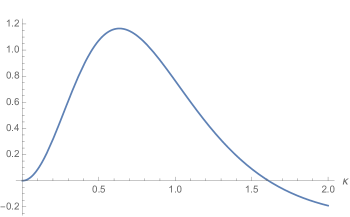
Figure 2. The graph of $i_{4}(\kappa)$ for $\kappa\in(0,2)$.

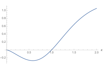
Figure 3. The graph of $i_{4}(1.61\kappa^{-1})$ for $\kappa\in(0,2)$.

It is difficult to analytically study the sign of $i_{4}$ further. On the other hand, a numerical evaluation of (3.19d) reveals a unique root $\kappa_{c}$, say, of $i_{4}$ over the interval $(0,\infty)$ (see Figure 2) such that $i_{4}(\kappa)>0$ if $0<\kappa<\kappa_{c}$ and it is negative if $\kappa_{c}<\kappa<\infty$. Upon close inspection (see Figure 3), moreover, $\kappa_{c}=1.610\dots$. We summarize the conclusion.

Corollary 3.3 (Critical wave number).

A sufficiently small, $2\pi/\kappa$-periodic wave train of (2.1)-(2.2) is modulationally unstable if $\kappa>\kappa_{c}$, where $\kappa_{c}=1.610\dots$ is a unique root of $i_{4}$ in (3.19d) over the interval $(0,\infty)$. It is spectrally stable to square integrable perturbations in the vicinity of the origin in $\mathbb{C}$ if $0<\kappa<\kappa_{c}$.

Corollary 3.3 qualitatively states the Benjamin-Feir instability of a Stokes wave. Fortuitously, the critical wave number compares reasonably well with that in [BH67, Whi67] and [BM95]. The critical wave number for the Whitham equation (see (1.3)) is $1.146\dots$; see [HJ15a], for instance.

We point out that the critical wave number in [BH67, Whi67] and [BM95] was determined by an approximation of the numerical value of some explicit function of $\kappa$, which seems difficult to calculate analytically. Therefore, it is not surprising that the proof of Corollary 3.3 ultimately relies on a numerical evaluation of the modulational instability index (3.18).

4. Stability and instability away from the origin

Let $\eta=\eta(a;\kappa,0,0)$, $u=u(a;\kappa,0,0)$, and $c=c(a;\kappa,0,0)$, for some $a\in\mathbb{R}$ and $|a|$ sufficiently small for some $\kappa>0$, denote a $2\pi/\kappa$-periodic wave train of (2.1)-(2.2) near the rest state, whose existence follows from Theorem 2.1. In the previous section, we studied the spectrum of the associated linearized operator in the vicinity of the origin in $\mathbb{C}$, whereby we determined its modulational stability and instability. We turn the attention to the spectral stability and instability away from the origin. Throughout the section, we employ the notation in the previous section.

4.1. Collision condition

Recall from Section 3.4 that

$$\mathcal{L}(\xi,0)\mathbf{e}(n+\xi,\pm)=i\omega(n+\xi,\pm)\mathbf{e}(n+\xi,\pm)\qquad\text{for $n\in\mathbb{Z}$ and $\xi\in[0,1/2]$},$$

where

$$\omega(n+\xi,\pm)=(n+\xi)(c_{\textrm{\tiny ww}}(\kappa)\pm c_{\textrm{\tiny ww}}(\kappa(n+\xi)))\quad\text{and}\quad\mathbf{e}(n+\xi,\pm)(z)=\begin{pmatrix}1\\ \mp c_{\textrm{\tiny ww}}(\kappa(n+\xi)\end{pmatrix}e^{inz}$$

for $\kappa>0$. Recall that $i\omega(0,\pm)=i\omega(\pm 1,-)=0$ and $i\omega(n+\xi,\pm)\neq 0$ otherwise. Moreover, no collisions take place among $i\omega(n+\xi,+)$’s or among $i\omega(n+\xi,-)$’s except at the origin. But

$$i\omega(n_{1}+\xi,-)=i\omega(n_{2}+\xi,+)\neq 0\qquad\text{for some $n_{1},n_{2}\in\mathbb{Z}$ and $\xi\in(0,1/2]$}$$

for some $\kappa>0$ if and only if

(4.1) $$(n_{1}+\xi)c_{\textrm{\tiny ww}}(\kappa(n_{1}+\xi))+(n_{2}+\xi)c(\kappa(n_{2}+\xi))=(n_{1}-n_{2})c_{\textrm{\tiny ww}}(\kappa).$$

We claim that $i\omega(n_{1}+\xi,-)$ and $i\omega(n_{2}+\xi,+)$ do not collide for any $n_{1}$, $n_{2}\in\mathbb{Z}$ such that $|n_{1}-n_{2}|=1$ and $\xi\in(0,1/2]$ for any $\kappa>0$. Suppose on the contrary that $i\omega(n_{1}+\xi,-)=i\omega(n_{2}+\xi,+)$ for some $n_{1}$, $n_{2}\in\mathbb{Z}$ such that $|n_{1}-n_{2}|=1$ and $\xi\in(0,1/2]$ for some $\kappa>0$. Assume for now $n_{1}=n_{2}+1$ and $n_{2}\geqslant 0$. Since $n_{2}+1+\xi\geqslant 1$ and since $zc_{\textrm{\tiny ww}}(z)>0$ and increases monotonically over the interval $(0,\infty)$, it follows that

$$(n_{2}+1+\xi)c_{\textrm{\tiny ww}}(\kappa(n_{2}+1+\xi))+(n_{2}+\xi)c_{\textrm{\tiny ww}}(\kappa(n_{2}+\xi))>c_{\textrm{\tiny ww}}(\kappa)$$

for any integer $n_{2}\geqslant 0$ and $\xi\in(0,1/2]$ for any $\kappa>0$. This contradicts (4.1). One may repeat the argument for $n_{1}$, $n_{2}<0$. This proves the claim.

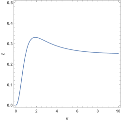
Figure 4. $\kappa$ vs. $\xi$ when $i\omega(2+\xi,-)$ and $i\omega(0+\xi,+)$ collide.

To proceed, a numerical evaluation of (4.1) reveals that $i\omega(n_{1}+\xi,-)=i\omega(n_{2}+\xi,+)$ for some $n_{1}$, $n_{2}\in\mathbb{Z}$ such that $|n_{1}-n_{2}|=2$ and $\xi\in(0,1/2]$ and for some $\kappa>0$ if and only if $n_{1}=2$ and $n_{2}=0$. Such a collision takes place for any $\kappa>0$ at some $\xi\in(0,1/2]$ depending on $\kappa$; see Figure 4.

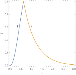
Figure 5. $\kappa$ vs. $\xi$ when $i\omega(n_{1}+\xi,-)$ and $i\omega(n_{2}+\xi,+)$ collide for $|n_{1}-n_{2}|=3$. Along Curve 1, $(n_{1},-)=(0,-)$ and $(n_{2},+)=(3,+)$ collide. Curve 2 represents the collision for $(-1,-)$ and $(-4,+)$.

Moreover, $i\omega(n_{1}+\xi,-)=i\omega(n_{2}+\xi,+)$ for some $n_{1}$, $n_{2}\in\mathbb{Z}$ such that $|n_{1}-n_{2}|=3$ and $\xi\in(0,1/2]$ for some $\kappa>0$ if and only if $n_{1}=0$ and $n_{2}=3$, or else $n_{1}=-1$ and $n_{2}=-4$. Together, such a collision takes place for any $\kappa>0$ at some $\xi\in(0,1/2]$ depending on $\kappa$; see Figure 5.

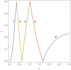
Figure 6. $\kappa$ vs. $\xi$ when $i\omega(n_{1}+\xi,-)$ and $i\omega(n_{2}+\xi,+)$ collide for $|n_{1}-n_{2}|=4$. Curves 1 through 5 represent the collisions for $(n_{1},-)=(0,-)$ and $(n_{2},+)=(4,+)$, $(-1,-)$ and $(-5,+)$, $(1,-)$ and $(5,+)$, $(-2,-)$ and $(-6,+)$, $(2,-)$ and $(6,+)$, respectively.

Continuing, a numerical evaluation of (4.1) reveals five collisions for $|n_{1}-n_{2}|=4$ when $(n_{1},-)=(0,-)$ and $(n_{2},+)=(4,+)$, $(-1,-)$ and $(-5,+)$, $(1,-)$ and $(5,+)$, $(-2,-)$ and $(-6,+)$, $(2,-)$ and $(6,+)$. Together, such a collision takes place for any $\kappa>0$ at some $\xi\in(0,1/2]$ depending on $\kappa$; see Figure 6.

$n_{1}$	$n_{2}$	$\xi$
$2$	$0$	0.261…
$1$	$5$	0.473…
$4$	$10$	0.184…
$6$	$13$	0.158…
$11$	$20$	0.250…
$14$	$24$	0.368…
$26$	$39$	0.006…

Table 1. Some $n_{1}$, $n_{2}$, and $\xi$ when $i\omega(n_{1}+\xi,-)$ and $i\omega(n_{2}+\xi,+)$ collide for $\kappa=1$ .

Indeed, for any $\kappa>0$ for any integer $n\geqslant 2$, it is possible to find $n_{1}$, $n_{2}\in\mathbb{Z}$ such that $i\omega(n_{1}+\xi,-)=i\omega(n_{2}+\xi,+)$ for some $\xi\in(0,1/2]$ and $|n_{1}-n_{2}|=n$. The number of collisions increases as $|n_{1}-n_{2}|$ increases. Therefore, $i\omega(n_{1}+\xi,-)$ and $i\omega(n+\xi,+)$ collide for infinitely many $n_{1}$, $n_{2}\in\mathbb{Z}$. In Table 1, we record some $n_{1}$, $n_{2}\in\mathbb{Z}$ ($n_{1}$, $n_{2}\geqslant 0$) and $\xi\in(0,1/2]$ for which $i\omega(n_{1}+\xi,-)$ and $i\omega(n_{2}+\xi,+)$ collide for $\kappa=1$.

The spectrum of the linear operator associated with the water wave problem in the finite depth (see [DO11, AN14], for instance, for details) contains infinitely many collisions of purely imaginary eigenvalues, which align with the collisions of $i\omega(n_{1}+\xi,-)$ and $i\omega(n_{2}+\xi,+)$ for (2.1)-(2.2). To compare, no eigenvalues of the linear operator for the Whitham equation (see (1.3)) collide other than at the origin; see [HJ15a], for instance, for details.

4.2. Signature calculation

The linear equation associated with (2.1)-(2.2) in the moving coordinate frame may be written in Hamiltonian form as

$$\partial_{t}\mathbf{u}=\begin{pmatrix}0&-\partial_{z}\\ -\partial_{z}&0\end{pmatrix}\delta H(\mathbf{u}),$$

where

$$H(\mathbf{u})=\int\Big{(}\frac{1}{2}\eta c_{\textrm{\tiny ww}}^{2}(\kappa|\partial_{z}|)\eta+\frac{1}{2}u^{2}-c\eta u\Big{)}~{}dz$$

and $\delta$ means variational differentiation. By the way, to the best of the authors’ knowledge, the Hamiltonian structure for (2.1)-(2.2) itself is not understood. In contrast, (1.9) and (1.2) (or (2.2)) are a Hamiltonian system. But the well-posedness for (1.9) is not understood, whence it is not suitable for the purpose of describing wave propagation. Note that the modulational instability proof in the previous section makes no use of Hamiltonian structure.

If $i\omega(n+\xi,\pm)$ for some $n\in\mathbb{Z}$ and $\xi\in[0,1/2]$ is a nonzero and purely imaginary eigenvalue of

$$\mathcal{L}(\xi,0)= \begin{pmatrix}0&-\partial_{z}+i\xi\\ -\partial_{z}+i\xi&0\end{pmatrix}e^{-i\xi z}\begin{pmatrix}-c_{\textrm{\tiny ww}}(\kappa)&1\\ c_{\textrm{\tiny ww}}^{2}(\kappa|\partial_{z}|)&-c_{\textrm{\tiny ww}}(\kappa)\end{pmatrix}e^{i\xi z}$$

$$= \begin{pmatrix}0&-\partial_{z}+i\xi\\ -\partial_{z}+i\xi&0\end{pmatrix}e^{-i\xi z}\delta^{2}H(\mathbf{0})e^{i\xi z}$$

(see (3.2) and (2.8)) then $e^{-i\xi z}\delta^{2}H(\mathbf{0})e^{i\xi z}$ defines a non-degenerate quadratic form on the associated eigenspace. If the eigenvalue is simple then the eigenspace is spanned by $\mathbf{e}(n+\xi,\pm)$, and

$$\langle e^{-i\xi z}\delta^{2}H(\mathbf{0})e^{i\xi z}\mathbf{e}(n+\xi,\pm),\mathbf{e}(n+\xi,\pm)\rangle= \mp 2c_{\textrm{\tiny ww}}(\kappa(n+\xi))(c_{\textrm{\tiny ww}}(\kappa)\pm c_{\textrm{\tiny ww}}(\kappa(n+\xi)))$$

$$= \mp 2\kappa\omega(n+\xi,\pm),$$

where $\langle\cdot\,,\cdot\rangle$ means the $L^{2}(\mathbb{T})\times L^{2}(\mathbb{T})$ inner product. This is either positive or negative, called the Krein signature. It is straightforward to verify that the Krein signature is positive for

(4.2) $$i\omega(n+\xi,-)\quad\text{for $n=-1$ or $n\geqslant 1$}\quad\text{and}\quad i\omega(n+\xi,+)\quad\text{for $n\geqslant 0$},$$

and negative for

(4.3) $$i\omega(n+\xi,-)\quad\text{for $n=0$ or $n\leqslant-2$}\quad\text{and}\quad i\omega(n+\xi,+)\quad\text{for $n\geqslant-1$}$$

for any $\xi\in[0,1/2]$. The eigenvalue remains simple and the Krein signature does not change, as parameters vary, so long as it does not collide with another eigenvalue; see [MS86], for instance, for details.

It is well known (see [MS86], for instance, and reference therein) that a necessary condition for spectral instability is that a pair of eigenvalues on the imaginary axis with opposite signature collide, unless they are at the origin. Note from (4.1), and (4.2), (4.3) that the signatures of all colliding eigenvalues of $\mathcal{L}(\xi,0)$ are opposite, unless they are at the origin. For the zero eigenvalue, the Krein signature calculation becomes inconclusive. But in the previous section, we made a spectral perturbation calculation and determined the modulational stability and instability.

4.3. Spetra of $\mathcal{L}(\xi_{0}+\xi,0)$ and $\mathcal{L}(\xi_{0},a)$

Let

$$i\omega(n_{1}+\xi_{0},-)=i\omega(n_{2}+\xi_{0},+)=:i\omega_{0}$$

for some $n_{1},n_{2}\in\mathbb{Z}$ and $\xi_{0}\in(0,1/2]$ for some $\kappa>0$, denote a nonzero and purely imaginary, colliding $L^{2}(\mathbb{T})\times L^{2}(\mathbb{T})$ eigenvalue of $\mathcal{L}(\xi_{0},0)$. Recall that $\mathbf{e}(n_{1}+\xi_{0},-)$ and $\mathbf{e}(n_{2}+\xi_{0},+)$ are the associated eigenfunctions, complex valued and orthogonal to each other. For $\xi$, $a\in\mathbb{R}$ and $|\xi|$, $|a|$ sufficiently small, we calculate the spectra of $\mathcal{L}(\xi_{0}+\xi,0)$ and $\mathcal{L}(\xi_{0},a)$ in the vicinity of $i\omega_{0}$ in $\mathbb{C}$.

For real valued functions, one must take $\pm\xi_{0}$ in pair (and, hence, $\pm i\omega_{0}$) and deal with four functions. But the spectral perturbation calculation in the following subsection involves complex valued operators anyway. Hence this is not worth the effort.

Notation

In the remaining of the section, $\kappa>0$ and $\xi_{0}\in(0,1/2]$ are suppressed for simplicity of notation, unless specified otherwise. We use

(4.4) $$c_{0}=c_{\textrm{\tiny ww}}(\kappa)\quad\text{and}\quad c_{n,\xi}=c_{\textrm{\tiny ww}}(\kappa(n+\xi_{0}+\xi))$$

and

(4.5) $$\mathbf{C}_{0}=\begin{pmatrix}c_{0}&1\\ 0&c_{0}\end{pmatrix}\quad\text{and}\quad\mathbf{C}_{n,\xi}=\begin{pmatrix}c_{0}&-1\\ -c^{2}_{n,\xi}&c_{0}\end{pmatrix}$$

for simplicity of notation.

For $\xi\in\mathbb{R}$ and $|\xi|$ sufficiently small, note from (3.4) that $i\omega(n_{1}+\xi_{0}+\xi,-)$ and $i\omega(n_{2}+\xi_{0}+\xi,+)$ are $L^{2}(\mathbb{T})\times L^{2}(\mathbb{T})$ eigenvalues of $\mathcal{L}(\xi_{0}+\xi,0)$ in the vicinity of $i\omega_{0}$ in $\mathbb{C}$, and

(4.6) $$\boldsymbol{\psi}_{1}(z):=\mathbf{e}(n_{1}+\xi_{0}+\xi,-)=\begin{pmatrix}1\\ c_{n_{1},\xi}\end{pmatrix}e^{in_{1}z},$$

$$\boldsymbol{\psi}_{2}(z):=\mathbf{e}(n_{2}+\xi_{0}+\xi,+)=\begin{pmatrix}1\\ -c_{n_{2},\xi}\end{pmatrix}e^{in_{2}z}$$

are the associated eigenfunctions, complex valued and orthogonal to each other.

As $|a|$ increases, two eigenvalues at $i\omega_{0}$ of $\mathcal{L}(\xi_{0},0)$ may move around and the associated eigenfunctions vary, analytically, from $\mathbf{e}(n_{1}+\xi_{0},-)$ and $\mathbf{e}(n_{2}+\xi_{0},+)$. For $a\in\mathbb{R}$ and $|a|$ sufficiently small, we calculate the small amplitude expansion of the eigenvalues and eigenfunctions of $\mathcal{L}(\xi_{0},a)$ up to terms of order $a$. To compare, Lemma 3.1 implies that as $a$ varies, zero persists to be an eigenvalue of $\mathcal{L}(0,a)$ and one may exploit the variations of (2.3) to find the associated eigenfunctions to any order in $a$. Let (by abuse of notation)

(4.7) $$\mathcal{L}(\xi_{0},a)\boldsymbol{\psi}_{k}(a)=\lambda(a)\boldsymbol{\psi}_{k}(a)\qquad\text{for $k=1,2$},$$

where

(4.8) $$\lambda(a)=i\omega_{0}+a\lambda_{1}+O(a^{2})\quad\text{and}\quad\boldsymbol{\psi}_{k}(a)(z)=\begin{pmatrix}1\\ \pm c_{n_{k},0}\end{pmatrix}e^{in_{k}z}+a\boldsymbol{\psi}_{k,1}(z)+O(a^{2})$$

as $a\to 0$, $\lambda_{1}\in\mathbb{C}$ and $\boldsymbol{\psi}_{1,1}$, $\boldsymbol{\psi}_{2,1}$ be $2\pi$ periodic. Note from (3.2) and (2.7) that

$$\mathcal{L}(\xi_{0},a)= e^{-i\xi_{0}z}\partial_{z}\begin{pmatrix}c_{0}&-1\\ -c_{\textrm{\tiny ww}}^{2}(\kappa|\partial_{z}|)&c_{0}\end{pmatrix}e^{i\xi_{0}z}-ae^{-i\xi_{0}z}\partial_{z}(\mathbf{C}_{0}\cos z)e^{i\xi_{0}z}+O(a^{2})$$

(4.9) $$=: \mathcal{L}_{0}+a\mathcal{L}_{1}+O(a^{2})$$

as $a\to 0$.

Substituting (4.8) and (4) into (4.7), we make an explicit calculation to arrive, at the order of $1$, at

(4.10) $$\mathcal{L}_{0}\begin{pmatrix}1\\ \pm c_{n_{k},0}\end{pmatrix}e^{in_{k}z}=i\omega_{0}\begin{pmatrix}1\\ \pm c_{n_{k},0}\end{pmatrix}e^{in_{k}z}\qquad\text{for $k=1$, $2$},$$

which holds true by hypothesis.

To proceed, at the order or $a$, we gather

$$\mathcal{L}_{0}\boldsymbol{\psi}_{k,1}+\mathcal{L}_{1}\begin{pmatrix}1\\ \pm c_{n_{k},0}\end{pmatrix}e^{in_{k}z}=i\omega_{0}\boldsymbol{\psi}_{k,1}+\lambda_{1}\begin{pmatrix}1\\ \pm c_{n_{k},0}\end{pmatrix}e^{in_{k}z}\qquad\text{for $k=1$, $2$}.$$

If $\boldsymbol{\psi}_{k,1}(z)=\sum_{m\in\mathbb{Z}}\mathbf{q}_{n_{k},m}e^{i(n_{k}+m)z}$ in the Fourier series then

(4.11) $$\begin{split}\sum_{m\in\mathbb{Z}}i(n_{k}+m+\xi_{0})\mathbf{C}_{n_{k}+m,0}\mathbf{q}_{n_{k},m}&e^{i(n_{k}+m)z}\\ -\frac{1}{2}\begin{pmatrix}c_{\textrm{\tiny ww}}(\kappa)\pm c_{n_{k},0}\\ \pm c_{\textrm{\tiny ww}}(\kappa)c_{n_{k},0}\end{pmatrix}(i(n_{k}+&1+\xi_{0})e^{i(n_{k}+1)z}+i(n_{k}-1+\xi_{0})e^{i(n_{k}-1)z})\\ =&i\omega_{0}\sum_{m\in\mathbb{Z}}\mathbf{q}_{n_{k},m}e^{i(n_{k}+m)z}+\lambda_{1}\begin{pmatrix}1\\ \pm c_{n_{k},0}\end{pmatrix}e^{in_{k}z}\end{split}$$

for $k=1$, $2$. Upon inspection, it follows that $\mathbf{q}_{n_{k},m}=\mathbf{0}$ unless $m=0$, $\pm 1$. We then take the $L^{2}(\mathbb{T})\times L^{2}(\mathbb{T})$ inner products of (4.11) and $\begin{pmatrix}1\\ 0\end{pmatrix}e^{in_{k}z}$, $\begin{pmatrix}0\\ 1\end{pmatrix}e^{in_{k}z}$, $k=1$, $2$, to arrive at

$$i(n_{k}+\xi_{0})\mathbf{C}_{n_{k},0}\mathbf{q}_{n_{k},0}=i\omega_{0}\mathbf{q}_{n_{k},0}+\lambda_{1}\begin{pmatrix}1\\ \pm c_{n_{k},0}\end{pmatrix}\qquad\text{for $k=1$, $2$}.$$

Note from (4.10) that $\lambda_{1}=0$. This agrees with the result in [AN14], for instance, for the water wave problem. Note that $\mathbf{q}_{n_{k},0}=\begin{pmatrix}1\\ \pm c_{n_{k},0}\end{pmatrix}$ up to the multiplication by a constant.

Continuing, we take the $L^{2}(\mathbb{T})\times L^{2}(\mathbb{T})$ inner products of (4.11) and $\begin{pmatrix}1\\ 0\end{pmatrix}e^{i(n_{1}\pm 1)z}$, $\begin{pmatrix}0\\ 1\end{pmatrix}e^{i(n_{1}\pm 1)z}$ to arrive at

$$(n_{1}\pm 1+\xi_{0})\Big{(}2\mathbf{C}_{n_{1}\pm 1,0}\mathbf{q}_{n_{1}\pm 1}-\mathbf{C}_{0}\begin{pmatrix}1\\ c_{n_{1},0}\end{pmatrix}\Big{)}=2\omega_{0}\mathbf{q}_{n_{1},\pm 1}.$$

A straightforward calculation then reveals that

(4.12) $$\mathbf{q}_{n_{1},\pm 1}= \frac{1}{2}\frac{n_{1}\pm 1+\xi_{0}}{(\omega_{0}-c_{0}(n_{1}\pm 1+\xi_{0}))^{2}-c^{2}_{n_{1}\pm 1,0}(n_{1}\pm 1+\xi_{0})^{2}}$$

$$\times\begin{pmatrix}c_{0}(n_{1}\pm 1+\xi_{0})(c_{0}+2c_{n_{1},0})-\omega_{0}(c_{0}+c_{n_{1},0})\\ (n_{1}\pm 1+\xi_{0})(c^{2}_{0}c_{n_{1},0}+c^{2}_{n_{1}\pm 1,0}(c_{0}+c_{n_{1},0}))-\omega_{0}c_{0}c_{n_{1},0}\end{pmatrix}.$$

We take the $L^{2}(\mathbb{T})\times L^{2}(\mathbb{T})$ inner products of (4.11) and $\begin{pmatrix}1\\ 0\end{pmatrix}e^{i(n_{2}\pm 1)z}$, $\begin{pmatrix}0\\ 1\end{pmatrix}e^{i(n_{2}\pm 1)z}$, likewise, and we make an explicit calculation to find

(4.13) $$\mathbf{q}_{n_{2},\pm 1}= \frac{1}{2}\frac{n_{2}\pm 1+\xi_{0}}{(\omega_{0}-c_{0}(n_{2}\pm 1+\xi_{0}))^{2}-c^{2}_{n_{2}\pm 1,0}(n_{2}\pm 1+\xi_{0})^{2}}$$

$$\times\begin{pmatrix}c_{0}(n_{2}\pm 1+\xi_{0})(c_{0}-2c_{n_{2},0})-\omega_{0}(c_{0}-c_{n_{2},0})\\ (n_{2}\pm 1+\xi_{0})(-c^{2}_{0}c_{n_{2},0}+c^{2}_{n_{2}\pm 1,0}(c_{0}-c_{n_{2},0}))+\omega_{0}c_{0}c_{n_{2},0}\end{pmatrix}.$$

We are able to calculate higher order terms in like manner. But the formulae become lengthy and complicated. We will investigate the details in a future publication.

To recapitulate, for $\xi\in\mathbb{R}$ and $|\xi|$ sufficiently small for $a=0$, the $L^{2}(\mathbb{T})\times L^{2}(\mathbb{T})$ spectrum of $\mathcal{L}(\xi_{0}+\xi,0)$ contains two purely imaginary eigenvalues $i\omega(n_{1}+\xi_{0}+\xi,-)$ and $i\omega(n_{2}+\xi_{0}+\xi,+)$ in the vicinity of $i\omega_{0}$ in $\mathbb{C}$, and (4.6) makes the associated eigenfunctions, which depend analytically on $\xi$. For $\xi=0$ for $a\in\mathbb{R}$ and $|a|$ sufficiently small, the spectrum of $\mathcal{L}(\xi_{0},a)$ contains two eigenvalues at $i\omega_{0}$ up to the order of $a$, and

(4.14) $$\boldsymbol{\psi}_{k}(a)=\begin{pmatrix}1\\ \pm c_{n_{k},0}\end{pmatrix}e^{in_{k}z}+a\mathbf{q}_{n_{k},1}e^{i(n_{k}+1)z}+a\mathbf{q}_{n_{k},-1}e^{i(n_{k}-1)z}+O(a^{2})\qquad\text{for $k=1$, $2$}$$

makes the associated eigenfunctions, which depend analytically on $a$, where $\mathbf{q}_{n_{k},\pm 1}$ for $k=1$, $2$ are in (4.12) and (4.13).

4.4. Spectra of $\mathcal{L}(\xi_{0}+\xi,a)$

For $\xi$, $a\in\mathbb{R}$ and $|\xi|$, $|a|$ sufficiently small, it follows from perturbation theory (see [Kat76, Section 4.3.5], for instance, for details) that the $L^{2}(\mathbb{T})\times L^{2}(\mathbb{T})$ spectrum of $\mathcal{L}(\xi_{0}+\xi,a)$ contains two eigenvalues in the vicinity of $i\omega_{0}$ in $\mathbb{C}$, and the associated eigenfunctions vary analytically from (4.6) and (4.14). Let (by abuse of notation)

(4.15) $$\boldsymbol{\psi}_{1}(\xi,a)(z)= \begin{pmatrix}1\\ c_{n_{1},\xi}\end{pmatrix}e^{in_{1}z}+a\mathbf{q}_{n_{1},1}e^{i(n_{1}+1)z}+a\mathbf{q}_{n_{1},-1}e^{i(n_{1}-1)z}+O(\xi^{2}a+a^{2}),$$

$$\boldsymbol{\psi}_{2}(\xi,a)(z)= \begin{pmatrix}1\\ -c_{n_{2},\xi}\end{pmatrix}e^{in_{2}z}+a\mathbf{q}_{n_{2},1}e^{i(n_{2}+1)z}+a\mathbf{q}_{n_{2},-1}e^{i(n_{2}-1)z}+O(\xi^{2}a+a^{2})$$

as $\xi$, $a\to 0$, where $\mathbf{q}_{n_{1},\pm 1}$ and $\mathbf{q}_{n_{2},\pm 1}$ are in (4.12) and (4.13). For $a=0$, note that $\boldsymbol{\psi}_{1}$ and $\boldsymbol{\psi}_{2}$ become (4.6). For $\xi=0$ they become (4.14). Hence $\boldsymbol{\psi}_{1}$ and $\boldsymbol{\psi}_{2}$ are the eigenfunctions associated with the eigenvalues of $\mathcal{L}(\xi_{0}+\xi,a)$ near $i\omega_{0}$ up to terms of order $a$ as $\xi$, $a\to 0$. It seems impossible to uniquely determine terms of order $\xi a$ in the eigenfunction expansion without an ad hoc orthogonality condition. Fortuitously, it turns out that they do not contribute to the spectral instability up to the order of $a$ as $\xi$, $a\to 0$. Hence we may neglect them in (4.15).

We proceed as in Section 3.6 and calculate (by abuse of notation)

(4.16) $$\mathbf{L}(\xi,a)= \begin{pmatrix}\dfrac{\langle\mathcal{L}(\xi_{0}+\xi,a)\boldsymbol{\psi}_{k}(\xi,a),\boldsymbol{\psi}_{\ell}(\xi,a)\rangle}{\langle\boldsymbol{\psi}_{k}(\xi,a),\boldsymbol{\psi}_{k}(\xi,a)\rangle}\end{pmatrix}_{k,\ell=1,2}$$

and

(4.17) $$\mathbf{I}(\xi,a)= \begin{pmatrix}\dfrac{\langle\boldsymbol{\psi}_{k}(\xi,a),\boldsymbol{\psi}_{\ell}(\xi,a)\rangle}{\langle\boldsymbol{\psi}_{k}(\xi,a),\boldsymbol{\psi}_{k}(\xi,a)\rangle}\end{pmatrix}_{k,\ell=1,2}$$

up to the order of $a$ as $\xi$, $a\to 0$. Throughout the subsection, $\langle\cdot\,,\cdot\rangle$ means the $L^{2}(\mathbb{T})\times L^{2}(\mathbb{T})$ inner product. For $\xi$, $a\in\mathbb{R}$ and $|\xi|$, $|a|$ sufficiently small, it follows from perturbation theory that the roots of $\det(\mathbf{L}-\lambda\mathbf{I})$ coincide with the eigenvalues of $\mathcal{L}(\xi_{0}+\xi,a)$ up to terms of order $a$.

We begin by calculating

$$\langle\boldsymbol{\psi}_{1},\boldsymbol{\psi}_{1}\rangle= 1+c^{2}_{n_{1},\xi}+O(\xi^{2}a+a^{2}),$$

$$\langle\boldsymbol{\psi}_{2},\boldsymbol{\psi}_{2}\rangle= 1+c^{2}_{n_{2},\xi}+O(\xi^{2}a+a^{2}),$$

and $\langle\boldsymbol{\psi}_{1},\boldsymbol{\psi}_{2}\rangle=\langle\boldsymbol{\psi}_{2},\boldsymbol{\psi}_{1}\rangle=0+O(\xi^{2}a+a^{2})$ as $\xi$, $a\to 0$, where $c_{n,\xi}$ is in (4.4). We then write

$$\mathcal{L}(\xi_{0}+\xi,a)=\mathcal{L}(\xi_{0}+\xi,0)- ae^{-i\xi_{0}z}\partial_{z}(\mathbf{C}_{0}\cos z)e^{i\xi_{0}z}$$

$$- i\xi ae^{-i\xi_{0}z}(\mathbf{C}_{0}\cos z)e^{i\xi_{0}z}+O(\xi^{2}a+a^{2})$$

as $\xi$, $a\to 0$ (see (3.2) and (2.7)), where $\mathbf{C}_{0}$ is in (4.5). We use (4.15), and we make a lengthy but explicit calculation to show that

$$\mathcal{L}\boldsymbol{\psi}_{k}= i\omega(n_{k}+\xi_{0}+\xi,\mp)\begin{pmatrix}1\\ \pm c_{n_{k},\xi}\end{pmatrix}e^{in_{k}z}$$

$$+ia(n_{k}+1+\xi_{0}+\xi)\mathbf{C}_{n_{k}+1,\xi}\mathbf{q}_{n_{k},1}e^{i(n_{k}+1)z}$$

$$+ia(n_{k}-1+\xi_{0}+\xi)\mathbf{C}_{n_{k}-1,\xi}\mathbf{q}_{n_{k},-1}e^{i(n_{k}-1)z}$$

$$-\frac{1}{2}ia\begin{pmatrix}c_{0}+c_{n_{k},\xi}\\ c_{0}c_{n_{k},\xi}\end{pmatrix}((n_{k}+1+\xi_{0}+\xi)e^{i(n_{k}+1)z}+(n_{k}-1+\xi_{0}+\xi)e^{i(n_{k}-1)z})$$

$$+O(\xi^{2}a+a^{2})$$

for $k=1$, $2$, as $\xi$, $a\to 0$, where $\mathbf{C}_{n,\xi}$ is in (4.5). Exact formulae of $\mathbf{C}_{n_{k}\pm 1,\xi}\mathbf{q}_{n_{k},\pm 1}$ are lengthy and tedious; see Section B for instance. But they do not influence the result. Hence we omit the details. Continuing, we take the $L^{2}(\mathbb{T})\times L^{2}(\mathbb{T})$ inner products of the above and (4.15), and we make a lengthy but explicit calculation to show that

$$\frac{\langle\mathcal{L}\boldsymbol{\psi}_{k},\boldsymbol{\psi}_{k}\rangle}{\langle\boldsymbol{\psi}_{k},\boldsymbol{\psi}_{k}\rangle}=i\omega(n_{k}+\xi_{0}+\xi,\mp)+O(\xi^{2}a+a^{2})$$

for $k=1$, $2$, and

$$\frac{\langle\mathcal{L}\boldsymbol{\psi}_{1},\boldsymbol{\psi}_{2}\rangle}{\langle\boldsymbol{\psi}_{1},\boldsymbol{\psi}_{1}\rangle}=\frac{\langle\mathcal{L}\boldsymbol{\psi}_{2},\boldsymbol{\psi}_{1}\rangle}{\langle\boldsymbol{\psi}_{2},\boldsymbol{\psi}_{2}\rangle}=0+O(\xi^{2}a+a^{2})$$

as $\xi,a\to 0$.

Together, (4.16) and (4.17) become

$$\mathbf{L}(\xi,a)=\begin{pmatrix}i\omega(n_{1}+\xi_{0}+\xi,-)&0\\ 0&i\omega(n_{2}+\xi_{0}+\xi,+)\end{pmatrix}+O(\xi^{2}a+a^{2})$$

and $\mathbf{I}(\xi,a)=\mathbf{I}+O(\xi^{2}a+a^{2})$ as $\xi$, $a\to 0$, where $\mathbf{I}$ means the $2\times 2$ identity matrix. Clearly, for $\xi$, $a\in\mathbb{R}$ and $|\xi|$, $|a|$ sufficiently small, the roots of $\det(\mathbf{L}-\lambda\mathbf{I})(\xi,a)$ are purely imaginary up to terms of order $a$. Therefore, a sufficiently small, periodic wave train of (2.1)-(2.2) is spectrally stable to square integrable perturbations away from the origin in $\mathbb{C}$ to the linear order in the amplitude parameter. To compare, it is spectrally unstable in the vicinity of the origin in $\mathbb{C}$ at the linear order in the amplitude parameter if the modulational instability takes place. Hence, the modulational instability dominates the spectral instability away from the origin for (2.1)-(2.2), if the latter takes place.

Numerical computations in [MMM⁺81, McL82, MS86, DO11, AN14], for instance, report that nonzero colliding eigenvalues of the linear operator for the water wave problem contribute to spectral instability as the amplitude increases. The results are implicit, but the growth rate of an unstable eigenvalue seems the steepest at the origin. For instance, for $(n_{1},-)=(2,-)$, $(n_{2},+)=(6,+)$ and the colliding eigenvalue at $i3.353\dots$ but for $a=0.245\dots$, the unstable eigenvalue grows like $a^{4}$; see [MS86], for instance, for details. But it is difficult to analytically find colliding eigenvalues away from the origin in $\mathbb{C}$ for $a\neq 0$.

In Section B, we calculate some higher order terms near the colliding eigenvalues for $(n_{1},-)=(2,-)$ and $(n_{2},+)=(0,+)$. Unfortunately, we do not detect spectral instability up to the orders of $\xi a$ and $a^{2}$. But the result seems to agree with that in [AN14], for instance, from a numerical computation for the physical problem.

5. Effects of surface tension

The results in the previous sections may be adapted to other related equations. We illustrate this for the full-dispersion shallow water equations in the presence of the effects of surface tension. That is,

(5.1) $$c_{\textrm{\tiny ww}}(\kappa;T):=\sqrt{(1+T\kappa^{2})\frac{\tanh\kappa}{\kappa}}$$

replaces (2.2), where $T$ is the coefficient of surface tension. Throughout the section, we employ the notation in Section 2 and Section 3.

Properties of $c_{\textrm{\tiny ww}}(\cdot\,;T)$

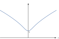
(a)    (b)  

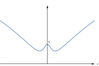
Figure 7. Schematic plots of $c_{\textrm{\tiny ww}}(\cdot\,;T)$ when (a) $T\geqslant 1/3$ and (b) $0<T<1/3$.

For any $T>0$, since

$$c_{\textrm{\tiny ww}}^{2}(\kappa;T)=(1+T\kappa^{2})c_{\textrm{\tiny ww}}^{2}(\kappa),$$

note from Section 2.1 that $c_{\textrm{\tiny ww}}^{2}(\cdot\,;T)$ is even and real analytic, and $c_{\textrm{\tiny ww}}^{2}(0;T)=1$. Moreover, $c_{\textrm{\tiny ww}}^{2}(|\partial_{x}|;T)$ may be regarded equivalent to $1+|\partial_{x}|$ in the $L^{2}$-Sobolev space setting. In particular, $c_{\textrm{\tiny ww}}^{2}(|\partial_{x}|;T):H^{s+1}(\mathbb{R})\to H^{s}(\mathbb{R})$ for any $s\in\mathbb{R}$.

When $T\geqslant 1/3$, note that $c_{\textrm{\tiny ww}}(\cdot\,;T)$ increases monotonically and unboundedly away from the origin. When $0<T<1/3$, on the other hand, $c_{\textrm{\tiny ww}}^{\prime}(0;T)=0$, $c_{\textrm{\tiny ww}}^{\prime\prime}(0;T)<0$ and $c_{\textrm{\tiny ww}}(\kappa;T)\to\infty$ as $\kappa\to\infty$. Hence $c_{\textrm{\tiny ww}}(\cdot\,;T)$ possesses a unique minimum over the interval $(0,\infty)$; see Figure 7.

Well-posedness

For any $T>0$, it follows from harmonic analysis techniques that the solution of the linear part of (2.1) and (5.1) acquires a $1/4$ derivative of “smoothness,” compared to the initial datum. By the way, for $T=0$, the solution does not possess smoothing effects. Nevertheless, it seems difficult to work out the well-posedness in spaces of low regularities. But, for the present purpose, it suffices to solve the Cauchy problem in some functional analytic setting. In Appendix A, we comment how to establish the local-in-time well-posedness for (2.1) and (5.1) in $H^{s}(\mathbb{R})\times H^{s+1/2}(\mathbb{R})$ for any $s>2$.

5.1. Existence of sufficiently small, periodic wave trains

Let $T>0$. We begin by discussing periodic wave trains of (2.1) and (5.1). That is, $\eta$ and $u$ are $2\pi$ periodic functions of $z:=\kappa(x-ct)$ for some $\kappa>0$, the wave number, for some $c>0$, the wave speed, and they solve

(5.2) $$-c\eta+u+u\eta=(1-c^{2})b_{1},$$

$$-cu+c_{\textrm{\tiny ww}}^{2}(\kappa|\partial_{z}|;T)\eta+\frac{1}{2}u^{2}=(1-c^{2})b_{2}$$

for some $b_{1}$, $b_{2}\in\mathbb{R}$; compare (2.3). For any $T>0$, note that

(5.3) $$c_{\textrm{\tiny ww}}^{2}(\kappa|\partial_{z}|;T):H^{k+1}(\mathbb{T})\to H^{k}(\mathbb{T})\qquad\text{for any $\kappa>0$\quad for any integer $k\geqslant 0$}.$$

Note that

(5.4) $$c_{\textrm{\tiny ww}}^{2}(\kappa|\partial_{z}|;T)e^{inz}=c_{\textrm{\tiny ww}}^{2}(n\kappa;T)e^{inz}\qquad\text{for $n\in\mathbb{Z}$};$$

compare (2.4) and (2.5).

Here the existence proof follows along the same line as that in Section 2. Hence we merely hit the main points. We use (2.11) whenever it is convenient to do so.

Lemma 5.1 (Regularity).

For any $T>0$, if $\eta$, $u\in H^{1}(\mathbb{T})$ solve (5.2) for some $c>0$, and $\kappa>0$, $b_{1}$, $b_{2}\in\mathbb{R}$ and if $1-\|\eta\|_{L^{\infty}(\mathbb{T})}\geqslant\epsilon>0$ for some $\epsilon$ then $\eta$, $u\in H^{\infty}(\mathbb{T})$.

Proof.

We rearrange (5.2) as

(5.5) $$u=\frac{1}{1+\eta}(c\eta+(1-c^{2})b_{1})\quad\text{and}\quad c_{\textrm{\tiny ww}}^{2}(\kappa|\partial_{z}|)\eta=cu-\frac{1}{2}u^{2}+(1-c^{2})b_{2}.$$

Since $u\in H^{1}(\mathbb{T})$ by hypothesis, it follows from the latter equation of (5.5), a Sobolev inequality, and (5.3) that $\eta\in H^{2}(\mathbb{T})$. Since $\frac{1}{1+\eta}:H^{2}(\mathbb{T})\to H^{2}(\mathbb{T})$ by hypothesis, it follows from the former equation of (5.5) that $u\in H^{2}(\mathbb{T})$. A bootstrap argument then completes the proof. Compare Lemma 2.2 and the proof. ∎

For any $T>0$, let (by abuse of notation) $\mathbf{f}:H^{1}(\mathbb{T})\times H^{1}(\mathbb{T})\times\mathbb{R}^{+}\times\mathbb{R}^{+}\times\mathbb{R}\times\mathbb{R}\to L^{2}(\mathbb{T})\times L^{2}(\mathbb{T})$ such that

$$\mathbf{f}(\mathbf{u},c;T,\kappa,b_{1},b_{2})=\begin{pmatrix}-c\eta+u+u\eta-(1-c^{2})b_{1}\\ -cu+c_{\textrm{\tiny ww}}^{2}(\kappa|\partial_{z}|;T)\eta+\frac{1}{2}u^{2}-(1-c^{2})b_{2}\end{pmatrix};$$

compare (2.12). It is well defined by (5.3) and a Sobolev inequality. We seek a solution $\mathbf{u}\in H^{1}(\mathbb{T})\times H^{1}(\mathbb{T})$, $c>0$, and $\kappa>0$, $b_{1}$, $b_{2}\in\mathbb{R}$ of

$$\mathbf{f}(\mathbf{u},c;T,\kappa,b_{1},b_{2})=\mathbf{0}$$

satisfying $1-\|\eta\|_{L^{\infty}(\mathbb{T})}\geqslant\epsilon>0$ for some $\epsilon$ and, by virtue of Lemma 5.1, a solution $\mathbf{u}\in H^{\infty}(\mathbb{T})\times H^{\infty}(\mathbb{T})$ of (5.2). We may repeat the argument in Section 2.4 to verity that $\mathbf{f}$ is a real analytic operator.

For any $T>0$, for any $c>0$, $\kappa>0$, $b_{1}$, $b_{2}\in\mathbb{R}$ and $|b_{1}|$, $|b_{2}|$ sufficiently small, note that $\mathbf{u}_{0}:=\begin{pmatrix}\eta_{0}\\ u_{0}\end{pmatrix}(c;T,\kappa,b_{1},b_{2})$ makes a constant solution of $\mathbf{f}(\mathbf{u},c;T,\kappa,b_{1},b_{2})=\mathbf{0}$ and, hence, (5.2), where $\eta_{0}$ and $u_{0}$ are in (2.14). It follows from the implicit function theorem that if non-constant solutions bifurcate from $\mathbf{u}=\mathbf{u}_{0}$ for some $c=c_{0}$ then, necessarily, (by abuse of notation)

$$\mathbf{L}_{0}:=\partial_{\mathbf{u}}\mathbf{f}(\mathbf{u}_{0},c_{0};T,\kappa,b_{1},b_{2}):H^{1}(\mathbb{T})\times H^{1}(\mathbb{T})\to L^{2}(\mathbb{T})\times L^{2}(\mathbb{T})$$

is not an isomorphism. This is not in general a sufficient condition, but note from Section 2 that bifurcation does take place, provided that the kernel of $\mathbf{L}_{0}$ is two dimensional. Note that

$$\mathbf{L}_{0}\mathbf{u}_{1}e^{inz}=\begin{pmatrix}u_{0}-c_{0}&1+\eta_{0}\\ c_{\textrm{\tiny ww}}^{2}(\kappa|\partial_{z}|;T)&u_{0}-c_{0}\end{pmatrix}\mathbf{u}_{1}e^{inz}\qquad\text{for $n\in\mathbb{Z}$}$$

for some nonzero $\mathbf{u}_{1}$ if and only if

$$(c_{0}-u_{0})^{2}=c_{\textrm{\tiny ww}}^{2}(n\kappa;T)(1+\eta_{0});$$

compare (2.16). For $b_{1}=b_{2}=0$ and, hence, $\eta_{0}=u_{0}=0$ by (2.14), it simplifies to $c_{0}=\pm c_{\textrm{\tiny ww}}(n\kappa;T)$. Without loss of generality, we restrict the attention to $n=1$ and we assume the $+$ sign. For $|b_{1}|$ and $|b_{2}|$ sufficiently small, we then make an explicit calculation to find (2.8), where $c_{\textrm{\tiny ww}}(\cdot\,;T)$ replaces $c_{\textrm{\tiny ww}}$.

When $T\geqslant 1/3$, since $c_{\textrm{\tiny ww}}(\kappa;T)<c_{\textrm{\tiny ww}}(n\kappa;T)$ for any $n=2,3,\dots$ pointwise in $\mathbb{R}$ (see Figure 7a), a straightforward calculation reveals that for any $\kappa>0$, $b_{1}$, $b_{2}\in\mathbb{R}$ and $|b_{1}|$, $|b_{2}|$ sufficiently small, the $H^{1}(\mathbb{T})\times H^{1}(\mathbb{T})$ kernel of $\mathbf{L}_{0}=\partial_{\mathbf{u}}\mathbf{f}(\mathbf{u}_{0},c_{0};T,\kappa,b_{1},b_{2})$ is two dimensional and spanned by $\mathbf{u}_{1}e^{\pm iz}$, where $\mathbf{u}_{1}$ is in (2.17) and $c_{\textrm{\tiny ww}}(\cdot\,;T)$ replaces $c_{\textrm{\tiny ww}}$. Hence, non-constant solutions bifurcate from $\mathbf{u}=\mathbf{u}_{0}$ and $c=c_{0}$.

When $0<T<1/3$, on the other hand, for any integer $n\geqslant 2$, it is possible to find some $\kappa$ such that $c_{\textrm{\tiny ww}}(\kappa;T)=c_{\textrm{\tiny ww}}(n\kappa;T)$ (see Figure 7b). If $c_{\textrm{\tiny ww}}(\kappa;T)\neq c_{\textrm{\tiny ww}}(n\kappa;T)$ for any $n=2,3,\dots$ then the kernel of $\mathbf{L}_{0}$ is likewise two dimensional. Hence, non-constant solutions bifurcate from $\mathbf{u}=\mathbf{u}_{0}$ and $c=c_{0}$. But if $c_{\textrm{\tiny ww}}(\kappa;T)=c_{\textrm{\tiny ww}}(n\kappa;T)$ for some integer $n\geqslant 2$, resulting in the resonance of the fundamental mode and the $n$-th harmonic, then the kernel is four dimensional.

To compare, for $T=0$, recall that $c_{\textrm{\tiny ww}}(\kappa;0)<c_{\textrm{\tiny ww}}(n\kappa;0)$ for any $n=2,3,\dots$ pointwise in $\mathbb{R}$ (see Figure 1). Hence, for any $\kappa>0$, $b_{1}$, $b_{2}\in\mathbb{R}$ and $|b_{1}|$, $|b_{2}|$ sufficiently small, the kernel is two dimensional.

To proceed, for any $T>0$, for any $\kappa>0$ satisfying

(5.6) $$c_{\textrm{\tiny ww}}(\kappa;T)\neq c_{\textrm{\tiny ww}}(n\kappa;T),\qquad n=2,3,\dots,$$

$b_{1}$, $b_{2}\in\mathbb{R}$ and $|b_{1}|$, $|b_{2}|$ sufficiently small, we may repeat the Lyapunov-Schmidt procedure in Section 2.6 to establish that a one parameter family of solutions of (5.2) exists, denoted (by abuse of notation) $\eta(a;T,\kappa,b_{1},b_{2})(z)$, $u(a;T,\kappa,b_{1},b_{2})(z)$, and $c(a;T,\kappa,b_{1},b_{2})$, near $\eta_{0}(T,\kappa,b_{1},b_{2})$, $u_{0}(T,\kappa,b_{1},b_{2})$, and $c_{0}(T,\kappa,b_{1},b_{2})$, for $a\in\mathbb{R}$ and $|a|$ sufficiently small. Note that $\eta$ and $u$ are $2\pi$ periodic and even in $z$, and they belong to $H^{\infty}(\mathbb{T})$. Note that $\eta$, $u$, and $c$ depend analytically on $a$, and $\kappa$, $b_{1}$, $b_{2}$. Moreover, we may repeat the small amplitude expansion in Section 2.7 to verify (2.7) and (2.8) as $a$, $b_{1}$, $b_{2}\to 0$, where $c_{\textrm{\tiny ww}}(\cdot\,;T)$ replaces $c_{\textrm{\tiny ww}}$. We omit the details.

If $c_{\textrm{\tiny ww}}(\kappa;T)=c_{\textrm{\tiny ww}}(n\kappa;T)$ for some integer $n\geqslant 2$ for some $\kappa>0$ then the proof in Section 2 breaks down. Nevertheless, one may employ the Lyapunov-Schmidt procedure in [Jon89], for instance, to prove the existence of sufficiently small, periodic wave trains of (2.1) and (5.1). But the modulational instability calculation becomes tedious, involving $6\times 6$ matrices. We do not discuss the details.

5.2. Modulational stability and instability

Let $T>0$. Let $\eta=\eta(a;T,\kappa,0,0)$, $u=u(a;T,\kappa,0,0)$, and $c=c(a;T,\kappa,0,0)$, for some $a\in\mathbb{R}$ and $|a|$ sufficiently small for some $\kappa>0$ satisfying (5.6), denote a $2\pi/\kappa$-periodic wave train of (2.1) and (5.1) near the rest state, whose existence follows from the previous subsection. We turn the attention to its modulational stability and instability. Recall from Section 3.3 that the modulational instability means that the $L^{2}(\mathbb{T})\times L^{2}(\mathbb{T})$ spectra of (by abuse of notation)

$$\mathcal{L}(\xi)(a;T,\kappa,0,0):=e^{-i\xi z}\partial_{z}\begin{pmatrix}c-u&-1-\eta\\ -c_{\textrm{\tiny ww}}^{2}(\kappa|\partial_{z}|;T)&c-u\end{pmatrix}(a;T,\kappa,0,0)e^{i\xi z}$$

are not contained in the imaginary axis in the vicinity of the origin for $\xi>0$ and small.

Here the modulational stability and instability proof follows along the same line as that in Section 3. Hence we merely hit the main points. In the sequel, $\kappa>0$ satisfying (5.6) is suppressed for simplicity of notation, unless specified otherwise. We use the notation of (3.3).

For any $T>0$ for $a=0$, a straightforward calculation reveals that (by abuse of notation)

$$\mathcal{L}(\xi,0)\mathbf{e}(n+\xi,\pm;T)=i\omega(n+\xi,\pm;T)\mathbf{e}(n+\xi,\pm;T)\qquad\text{for $n\in\mathbb{Z}$ and $\xi\in[0,1/2]$},$$

where

$$\omega(n+\xi,\pm;T)=(n+\xi)(c_{\textrm{\tiny ww}}(\kappa;T)\pm c_{\textrm{\tiny ww}}(\kappa(n+\xi);T))$$

and $\mathbf{e}(n+\xi,\pm;T)(z)=\begin{pmatrix}1\\ \mp c_{\textrm{\tiny ww}}(\kappa(n+\xi);T)\end{pmatrix}e^{inz}$; compare (3.4) and (3.5). Note that

$$\omega(0,+;T)=\omega(0,-;T)=\omega(1,-;T)=\omega(-1,-;T)=0.$$

Since $c_{\textrm{\tiny ww}}(\kappa;T)\neq c_{\textrm{\tiny ww}}(n\kappa;T)$ for any $n=2,3,\dots$ by hypothesis, a straightforward calculation reveals that zero is an $L^{2}(\mathbb{T})\times L^{2}(\mathbb{T})$ eigenvalue of $\mathcal{L}(0,0)$ with algebraic and geometric multiplicity four. Moreover, (3.6) makes the associated eigenfunctions, where $c_{\textrm{\tiny ww}}(\cdot\,;T)$ replaces $c_{\textrm{\tiny ww}}$.

For $\xi=0$ for $a\in\mathbb{R}$ and $|a|$ sufficiently small, one may repeat the proof of Lemma 3.1 to establish that zero is an $L^{2}(\mathbb{T})\times L^{2}(\mathbb{T})$ eigenvalue of $\mathcal{L}(0,a)$ with algebraic multiplicity four and geometric multiplicity three. Moreover, (3.9) makes the associated eigenfunctions, where $c_{\textrm{\tiny ww}}(\cdot\,;T)$ replaces $c_{\textrm{\tiny ww}}$. We omit the details.

For any $T>0$, for $\xi>0$, $a\in\mathbb{R}$ and $\xi$, $|a|$ sufficiently small, one may then proceed as in Section 3.6 and calculate (3.11) and (3.12) up to terms of orders of $\xi^{2}$, $\xi a$, and $a$, where $\boldsymbol{\phi}_{1}$, $\boldsymbol{\phi}_{2}$, $\boldsymbol{\phi}_{3}$, $\boldsymbol{\phi}_{4}$ are in (3.10) but $c_{\textrm{\tiny ww}}(\cdot\,;T)$ replaces $c_{\textrm{\tiny ww}}$. It follows from perturbation theory (see [Kat76, Section 4.3.5], for instance, for details) that the roots of $\det(\mathbf{L}-\lambda\mathbf{I})(\xi,a)$ coincide with the $L^{2}(\mathbb{T})\times L^{2}(\mathbb{T})$ spectrum of $\mathcal{L}(\xi,a)$ up to terms of orders $\xi^{2}$ and $a$ as $\xi$, $a\to 0$. We then repeat the argument of Section 3.7 and derive a modulational instability index for (2.1) and (5.1).

Theorem 5.2 (Modulational instability index).

For any $T>0$ and $T\neq 1/3$ for any $\kappa>0$ satisfying $c_{\emph{\tiny ww}}(\kappa;T)\neq c_{\emph{\tiny ww}}(n\kappa;T)$ for $n=2,3,\dots$, a sufficiently small, $2\pi/\kappa$-periodic wave train of (2.1) and (5.1) is modulationally unstable, provided that

$$\Delta(\kappa;T):=\Big{(}\frac{i_{1}i_{2}}{i_{3}}i_{4}\Big{)}(\kappa;T)<0,$$

where

$$i_{1}(\kappa;T)= (\kappa c_{\emph{\tiny ww}}(\kappa;T))^{\prime\prime},$$

$$i_{2}(\kappa;T)= ((\kappa c_{\emph{\tiny ww}}(\kappa;T))^{\prime})^{2}-1,$$

$$i_{3}(\kappa;T)= c_{\emph{\tiny ww}}^{2}(\kappa;T)-c_{\emph{\tiny ww}}^{2}(2\kappa;T),$$

and

$$i_{4}(\kappa;T)= 3c_{\emph{\tiny ww}}^{2}(\kappa;T)+5c_{\emph{\tiny ww}}^{4}(\kappa;T)-2c_{\emph{\tiny ww}}^{2}(2\kappa;T)(c_{\emph{\tiny ww}}^{2}(\kappa;T)+2)$$

$$+18\kappa(c_{\emph{\tiny ww}}^{3}c_{\emph{\tiny ww}}^{\prime})(\kappa;T)+\kappa^{2}(c_{\emph{\tiny ww}}^{\prime})^{2}(\kappa;T)(5c_{\emph{\tiny ww}}^{2}(\kappa;T)+4c_{\emph{\tiny ww}}^{2}(2\kappa;T));$$

$c_{\emph{\tiny ww}}(\kappa,T)$ is in (5.1). It is spectrally stable to square integrable perturbations in the vicinity of the origin otherwise.

The proof is nearly identical to that of Theorem 3.2. Hence we omit the details. If $T=1/3$ then the result becomes inconclusive.

Theorem 5.2 elucidates four resonance mechanisms which contribute to the sign change in $\Delta$ and, ultimately, the change in the modulational stability and instability for (2.1) and (5.1). When $T=0$, note that $\Delta(\kappa;0)$ becomes (3.18). But for $T>0$, several differences are present. For instance, $i_{2}(\kappa;0)<0$ for any $\kappa>0$, but the effects of surface tension are to increase the group velocity, and they may do so to the extent that $i_{2}$ changes the sign.

When $T>1/3$, since $c_{\textrm{\tiny ww}}(\kappa;T)$ and $(\kappa c_{\textrm{\tiny ww}}(\kappa;T))^{\prime}$ increase monotonically over the interval $(0,\infty)$ and since $(\kappa c_{\textrm{\tiny ww}}(\kappa;T))^{\prime}$ does not possess an extremum by brutal force, $i_{1}$, $i_{2}$, $i_{3}$ in Theorem 5.2 do not vanish over the interval $(0,\infty)$. Moreover, a numerical evaluation reveals that $i_{4}$ changes the sign once over the interval $(0,\infty)$. Together, a sufficiently small, periodic wave train of (2.1) and (5.1) is modulationally unstable, provided that the wave number is greater than a critical value, and it is modulationally stable otherwise; compare Corollary 3.3. Furthermore, a numerical evaluation reveals that the critical wave number $\kappa_{c}(T)$, say, satisfies

$$\lim_{T\to\infty}\sqrt{T}\kappa_{c}(T)\approx 1.054.$$

When $0<T<1/3$, on the other hand, a straightforward calculation reveals that $(\kappa c_{\textrm{\tiny ww}}(\kappa;T))^{\prime}$ achieves a unique minimum over the interval $(0,\infty)$. Moreover, $(\kappa c_{\textrm{\tiny ww}}(\kappa;T))^{\prime}=1$ and $c_{\textrm{\tiny ww}}(\kappa;T)=c_{\textrm{\tiny ww}}(2\kappa;T)$ each takes one transvere root over the interval $(0,\infty)$. Hence, $i_{1}$ through $i_{4}$ each contributes to the change in the modulational stability and instability.

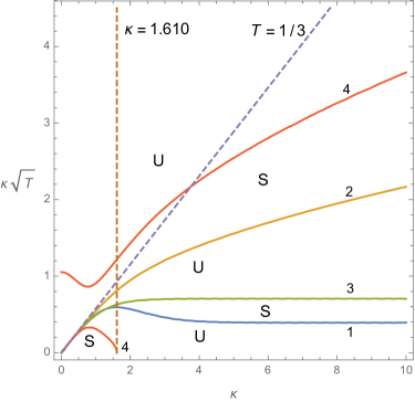
Figure 8. Stability diagram for sufficiently small, periodic wave trains of (2.1) and (5.1). To interpret, for any $T>0$, one must envision a line through the origin with slope $T$. “S” and “U” denote stable and unstable regions. Solid curves represent roots of the modulational instability index and are labeled according to their mechanism.

Figure 8 illustrates in the $\kappa$ versus $\kappa\sqrt{T}$ plane the regions where a sufficiently small, periodic wave train of (2.1) and (5.1) is modulationally stable and unstable. Along Curve 1, $i_{1}(\kappa;T)=0$ and the group speed achieves an extremum at the wave number $\kappa$. Curve 2 is associated with $i_{2}(\kappa;T)=0$, along which the group speed coincides with the phase speed in the long wave limit as $\kappa\to 0$, resulting in the resonance of short and long waves. In the deep water limit, as $\kappa\to\infty$ while $\kappa\sqrt{T}$ is fixed, it is asymptotic to $\kappa=\frac{9}{4}\kappa^{2}T-\frac{3}{4}$. Curve 3 is associated with $i_{3}(\kappa;T)=0$, along which the phase speeds of the fundamental mode and the second harmonic coincide, resulting in the second harmonic resonance. In the deep water limit, it is asymptotic to $k^{2}T=\frac{1}{2}$. Moreover along Curve 4, $i_{4}$ vanishes as a result of a rather complicated balance of the dispersion and nonlinear effects. The “lower” branch of Curve 4 passes through $\kappa=1.160\dots$, the critical wave number when $T=0$; see Corollary 3.3. The “upper” branch passes through $\kappa\sqrt{T}=1.054\dots$, the large surface tension limit in [Kaw75], for instance.

The result qualitatively agrees with those in [Kaw75] and [DR77], for instance, from formal asymptotic expansions for the water wave problem. To compare, the Whitham equation (see (1.3)) in the presence of the effects of surface tension fails to predict the critical wave number in the large surface tension limit; see [HJ15b], for instance, for details. Perhaps, this is because the Whitham equation neglects many “higher order” nonlinearities of the physical problem. It is fortuitous that the full-dispersion shallow water equations proposed herein includes more physically realistic nonlinearities to predict all resonances in gravity capillary waves.

Note that along Curve 3, the modulational instability index becomes singular. It is interesting to justify the resonant interactions in [McG70a, McG70b], for instance, from formal asymptotic expansions for the physical problem.

Acknowledgements

The authors thank Bernard Deconinck, Mariana Haragus, Mathew Johnson, Hanrik Kalisch, and Olga Trichenko for helpful discussions.

VMH is supported by the National Science Foundation grant CAREER DMS-1352597, an Alfred P. Sloan research fellowship, the Arnold O. Beckman research award RB14100 of the Office of the Vice Chancellor for Research and a Beckman fellowship of the Center for Advanced Study at the University of Illinois at Urbana-Champaign. AKP is supported by CAREER DMS-1352597 and RB14100.

Appendix A Well-posedness

We discuss the solvability of the Cauchy problem associated with (2.1)-(2.2) or, equivalently,

(A.1) $$\partial_{t}\eta+\partial_{x}u+\partial_{x}(u\eta)=0,$$

$$\partial_{t}u-\mathcal{H}\eta+\gamma^{2}(|\partial_{x}|)\eta+u\partial_{x}u=0.$$

For $v\in L^{2}(\mathbb{R})$, the Hilbert transform of $v$ is written $\mathcal{H}v$ and defined in the Fourier space as

$$\widehat{\mathcal{H}v}(\kappa)=-i(\text{sgn}\,\kappa)\widehat{v}(\kappa).$$

Since

$$|\text{sgn}\,\kappa-\tanh\kappa|\leqslant e^{-|\kappa|}\qquad\text{pointwise in $\mathbb{R}$}$$

by brutal force (see also [Yos82], for instance),

(A.2) $$\|\gamma^{2}(|\partial_{x}|)v\|_{H^{s}(\mathbb{R})}\leqslant C\|v\|_{L^{2}(\mathbb{R})}\qquad\text{for any $s\geqslant 0$}$$

for some constant $C>0$ independent of $v$.

Theorem A.1 (Local-in-time well-posedness).

For any $s>2$ for any $\eta_{0}\in H^{s}(\mathbb{R})$ and $u_{0}\in H^{s+1/2}(\mathbb{R})$, a unique solution, denoted $\eta(t)=\eta(\cdot,t)$ and $u(t)=u(\cdot,t)$, of (A.1)-(A.2),

$$\eta(\cdot,0)=\eta_{0}\quad\text{and}\quad u(\cdot,0)=u_{0},$$

exists in $H^{s}(\mathbb{R})\times H^{s+1/2}(\mathbb{R})$ over the interval $[0,t_{\emph{\Tiny LWP}})$ for some $t_{\emph{\Tiny LWP}}>0$. Moreover, $(\eta_{0},u_{0})\mapsto(\eta(t),u(t))$ is continuous for any $t\in[0,t_{\emph{\Tiny LWP}})$.

The proof follows along the same line as the argument in [Kat83], for instance. The main difference is how one establishes an a priori bound. The same proof works in the presence of the effects of surface tension, for which

$$\partial_{t}u+(1-T\partial_{x}^{2})(-\mathcal{H}+\gamma^{2}(|\partial_{x}|))\eta+u\partial_{x}u=0$$

replaces the latter equation of (A.1). The same proof works in the periodic setting.

Preliminaries

Note that $\|\mathcal{H}v\|_{L^{2}(\mathbb{R})}=\|v\|_{L^{2}(\mathbb{R})}$ and $\mathcal{H}^{2}=-1$. Note that $|\partial_{x}|:=\mathcal{H}\partial_{x}$ is self adjoint, and

$$\int^{\infty}_{-\infty}(v^{2}+u|\partial_{x}|v)~{}dx$$

is equivalent to $\|v\|_{H^{1/2}(\mathbb{R})}^{2}$. Moreover, commutators of $\mathcal{H}$ and $|\partial_{x}|$ are “smoothing.”

Lemma A.2 (Smoothing).

(A.3) $$\int^{\infty}_{-\infty}fv|\partial_{x}|v~{}dx\leqslant C\|f\|_{H^{3/2+}(\mathbb{R})}\|v\|_{H^{1/2}(\mathbb{R})}^{2}\quad\text{and}\quad\int^{\infty}_{-\infty}f(\partial_{x}v)\mathcal{H}\partial_{x}v~{}dx\leqslant C\|f\|_{H^{5/2+}(\mathbb{R})}\|v\|_{L^{2}(\mathbb{R})}^{2}$$

for some constant $C>0$ independent of $f$ and $v$.

Proof.

Note that $|\partial_{x}|^{1/2}$ is self adjoint, and we calculate that

$$\int fv|\partial_{x}|u~{}dx=\int f(|\partial_{x}|^{1/2}v)^{2}~{}dx+\int(|\partial_{x}|^{1/2}[|\partial_{x}|^{1/2},f]v)v~{}dx.$$

Clearly, the first term of the right side is bounded by $\|f\|_{L^{\infty}(\mathbb{R})}\||\partial_{x}|^{1/2}v\|_{L^{2}(\mathbb{R})}^{2}$. We claim that the second term of the right side is bounded by $\||\kappa|\widehat{f}\|_{L^{1}(\mathbb{R})}\|v\|_{H^{1/2}(\mathbb{R})}^{2}$ up to the multiplication by a constant. Indeed, since

$$(|\partial_{x}|^{1/2}[|\partial_{x}|^{1/2},f]v)\,\widehat{}\,(\kappa)=\frac{1}{\sqrt{2\pi}}\int^{\infty}_{-\infty}|\kappa|^{1/2}(|\kappa|^{1/2}-|\kappa_{1}|^{1/2})\widehat{f}(\kappa-\kappa_{1})\widehat{v}(\kappa_{1})~{}d\kappa_{1}$$

and since $|\kappa|^{1/2}||\kappa|^{1/2}-|\kappa_{1}|^{1/2}|\leqslant C|\kappa-\kappa_{1}|$ for any $\kappa,\kappa_{1}\in\mathbb{R}$ for some constant $C>0$ by brutal force (see also [Yos82], for instance), it follows from Young’s inequality and the Parseval theorem that

$$\||\partial_{x}|^{1/2}[|\partial_{x}|^{1/2},f]v\|_{L^{2}(\mathbb{R})}\leqslant C\||\kappa|\widehat{f}\|_{L^{1}(\mathbb{R})}\|v\|_{L^{2}(\mathbb{R})}$$

for some constant $C>0$ independent of $f$ and $v$. Hölder’s inequality then proves the claim. The first inequality of (A.3) follows by a Sobolev inequality.

Note that $\mathcal{H}$ is skew adjoint, and we calculate that

$$\int f(\partial_{x}v)|\partial_{x}|v~{}dx= -\int f(\mathcal{H}\partial_{x}v)\partial_{x}v~{}dx-\int([\mathcal{H},f]\partial_{x}v)\partial_{x}v~{}dx$$

$$= -\frac{1}{2}\int([\mathcal{H},f]\partial_{x}v)\partial_{x}v~{}dx.$$

Since

$$(\partial_{x}[\mathcal{H},f]\partial_{x}v)\,\widehat{}\,(\kappa)=-\frac{1}{\sqrt{2\pi}}\int^{\infty}_{-\infty}\kappa(\text{sgn}(\kappa)-\text{sgn}(\kappa_{1}))\widehat{f}(\kappa-\kappa_{1})\kappa_{1}\widehat{v}(\kappa_{1})~{}d\kappa_{1}$$

and since $|\kappa|+|\kappa_{1}|=\kappa\,\text{sgn}\kappa+\kappa_{1}\text{sgn}\kappa_{1}\leqslant|\kappa-\kappa_{1}|$ whenever $\text{sgn}\kappa\neq\text{sgn}\kappa_{1}$ by brutal force (see also [Yos82], for instance), it follows from Young’s inequality and the Parseval theorem that

$$\|\partial_{x}[\mathcal{H},f]\partial_{x}v\|_{L^{2}(\mathbb{R})}\leqslant C\||\kappa|^{2}\widehat{f}\|_{L^{1}(\mathbb{R})}\|v\|_{L^{2}(\mathbb{R})}$$

for some constant $C>0$ independent of $f$ and $v$. Hölder’s inequality and a Sobolev inequality then prove the second inequality of (A.3). This completes the proof. ∎

A priori bound

For $k\geqslant 1$ an integer, let

(A.4) $$E_{k}^{2}(t)=\frac{1}{2}\|\eta\|_{L^{2}(\mathbb{R})}^{2}(t)+\frac{1}{2}\|u\|_{L^{2}(\mathbb{R})}^{2}(t)+\sum_{\ell=1}^{k}e_{\ell}^{2}(t),$$

where

(A.5) $$e_{\ell}^{2}(t)=\frac{1}{2}\int^{\infty}_{-\infty}((\partial_{x}^{\ell}\eta(t))^{2}+(\partial_{x}^{\ell}u(t))|\partial_{x}|(\partial_{x}^{\ell}u(t)))~{}dx.$$

Clearly, $E_{k}(t)$ is equivalent to $\|\eta\|_{H^{k}(\mathbb{R})}(t)+\|u\|_{H^{k+1/2}(\mathbb{R})}(t)$.

Lemma A.3 (A priori bound).

For any integer $k\geqslant 2$ if $\eta\in H^{k}(\mathbb{R})$ and $u\in H^{k+1/2}(\mathbb{R})$ solve (A.1)-(A.2) over the interval $[0,t_{0})$ for some $t_{0}>0$ then

(A.6) $$E_{k}(t)\leqslant\frac{E_{k}(0)}{1-CE_{k}(0)t}\qquad\text{for any $t\in[0,t_{1}]$}$$

for some constant $C>0$ independent of $\eta$ and $u$ for some $t_{1}\in(0,t_{0})$ depending on $E_{k}(0)$. Moreover,

(A.7) $$\|\eta\|_{H^{k}(\mathbb{R})}(t)+\|u\|_{H^{k+1/2}(\mathbb{R})}(t)\leqslant C(t,\|\eta\|_{H^{k}(\mathbb{R})}(0),\|u\|_{H^{k+1/2}(\mathbb{R})}(0))$$

for any $t\in[0,t_{1}]$.

Proof.

For $\ell\geqslant 1$ an integer, we differentiate (A.5) with respect to $t$ and use (A.1) to arrive at that

$$\frac{de_{\ell}^{2}}{dt}= \int((\partial_{x}^{\ell}\partial_{t}\eta)(\partial_{x}^{\ell}\eta)+(\partial_{x}^{\ell}\partial_{t}u)|\partial_{x}|(\partial_{x}^{\ell}u))~{}dx$$

$$= -\int\partial_{x}^{\ell}(\partial_{x}u+\partial_{x}(u\eta))(\partial_{x}^{\ell}\eta)~{}dx-\int\partial_{x}^{\ell}(-\mathcal{H}\eta+\gamma^{2}(|\partial_{x}|)\eta+u\partial_{x}u)|\partial_{x}|(\partial_{x}^{\ell}u)~{}dx$$

$$=: (I)+(II)$$

over the interval $(0,t_{0})$. An integration by parts leads to that

(A.8) $$(I)= -\int(\partial_{x}^{\ell+1}u)(\partial_{x}^{\ell}\eta)~{}dx+\Big{(}\ell+\frac{1}{2}\Big{)}\int(\partial_{x}u)(\partial_{x}^{\ell}\eta)^{2}~{}dx$$

$$-\int(\partial_{x}^{\ell+1}(u\eta)-u(\partial_{x}^{\ell+1}\eta)-(\ell+1)(\partial_{x}u)(\partial_{x}^{\ell}\eta))(\partial_{x}^{\ell}\eta)~{}dx.$$

Recall $|\partial_{x}|=\mathcal{H}\partial_{x}$. Since $\mathcal{H}$ is skew adjoint and $\mathcal{H}^{2}=-1$, moreover,

(A.9) $$(II)= -\int(\partial_{x}^{\ell+1}\eta)(\partial_{x}^{\ell}u)~{}dx-\int(\mathcal{H}\partial_{x}^{\ell+1}\gamma^{2}(|\partial_{x}|)\eta)(\partial_{x}^{\ell}u)~{}dx$$

$$-\int u(\partial_{x}^{\ell+1}u)\mathcal{H}(\partial_{x}^{\ell+1}u)~{}dx-\ell\int(\partial_{x}u)(\partial_{x}^{\ell}u)(\mathcal{H}\partial_{x}^{\ell+1}u)~{}dx$$

$$-\int(\partial_{x}^{\ell}(u\partial_{x}u)-u(\partial_{x}^{\ell+1}u)-\ell(\partial_{x}u)(\partial_{x}^{\ell}u))|\partial_{x}|(\partial_{x}^{\ell}u)~{}dx.$$

Note that the first term of the right side of (A.8) and the first term of the right side of (A.9) cancel each other when added together after an integration by parts. Note that the second term of the right side of (A.8) is bounded by $(\ell+\frac{1}{2})\|\partial_{x}u\|_{L^{\infty}(\mathbb{R})}\|\partial_{x}^{\ell}\eta\|_{L^{2}(\mathbb{R})}^{2}$ and the last term of the right side of (A.8) is bounded by $\|u\|_{H^{\ell}(\mathbb{R})}\|\partial_{x}^{\ell}\eta\|_{L^{2}(\mathbb{R})}^{2}$ up to the multiplication by a constant by the Leibniz rule. Moreover, note that the second term of the right side of (A.9) is bounded by $\|\eta\|_{L^{2}(\mathbb{R})}\|\partial_{x}^{\ell}u\|_{L^{2}(\mathbb{R})}$ by (A.2), the third and the fourth terms of the right side of (A.9) are bounded by $\|u\|_{H^{5/2+}(\mathbb{R})}\|\partial_{x}^{\ell}u\|_{H^{1/2}(\mathbb{R})}^{2}$ by (A.3). Note that for $\ell\geqslant 2$, the last term of the right side of (A.9) is bounded by $\|u\|_{H^{\ell+1/2}(\mathbb{R})}^{2}\||\partial_{x}|^{1/2}\partial_{x}^{\ell}u\|_{L^{2}(\mathbb{R})}$ up to the multiplication by a constant by the Leibniz rule and a Sobolev inequality. Together,

(A.10) $$\frac{de_{\ell}^{2}}{dt}\leqslant C(1+\|u\|_{H^{5/2+}(\mathbb{R})}+\|u\|_{H^{\ell+1/2}(\mathbb{R})})(\|\eta\|_{H^{\ell}(\mathbb{R})}^{2}+\|u\|_{H^{\ell+1/2}(\mathbb{R})}^{2})$$

for any integer $\ell\geqslant 2$ over the interval $(0,t_{0})$, for some constant $C>0$ independent of $\eta$ and $u$.

To proceed, we make an explicit calculation to show that

(A.11) $$\frac{1}{2}\frac{d}{dt}\|\eta\|_{L^{2}(\mathbb{R})}^{2}= -\int(\partial_{x}u+\partial_{x}(u\eta))\eta~{}dx$$

$$\leqslant \|\partial_{x}u\|_{L^{2}(\mathbb{R})}\|\eta\|_{L^{2}(\mathbb{R})}+\frac{1}{2}\|\partial_{x}u\|_{L^{\infty}(\mathbb{R})}\|\eta\|_{L^{2}(\mathbb{R})}^{2},$$

(A.12) $$\frac{1}{2}\frac{d}{dt}\|u\|_{L^{2}}^{2}= \int(\mathcal{H}\eta-\gamma^{2}(|\partial_{x}|)\eta-u\partial_{x}u)u~{}dx$$

$$\leqslant 2\|\eta\|_{L^{2}(\mathbb{R})}\|u\|_{L^{2}(\mathbb{R})}+\|\partial_{x}u\|_{L^{\infty}(\mathbb{R})}\|u\|_{L^{2}(\mathbb{R})}^{2}$$

over the interval $(0,t_{0})$. Here the first equalities of (A.11) and (A.12) use (A.1). Adding (A.10) through (A.12), we deduce that

$$\frac{dE_{k}}{dt}\leqslant CE_{k}^{2}$$

for any integer $k\geqslant 2$ over the interval $(0,t_{0})$, for some constant $C>0$ independent of $\eta$ and $u$. We then deduce (A.6) because it invites a solution until the time $t_{1}=(CE_{k}(0))^{-1}$. Moreover, we deduce (A.7) because $E_{k}(t)$ is equivalent to $\|\eta\|_{H^{k}(\mathbb{R})}(t)+\|u\|_{H^{k+1/2}(\mathbb{R})}(t)$. This completes the proof. ∎

Appendix B Collision of $(2,-)$ and $(0,+)$

Throughout the section, we employ the notation in Section 3 and Section 4. In particular, we use the notation of (3.3), and (4.4), (4.5) for simplicity of notation. Let

$$i\omega(2+\xi_{0},-)=i\omega(0+\xi_{0},+)=:i\omega_{0}$$

for some $\xi_{0}\in(0,1/2]$ denote a nonzero and purely imaginary, colliding $L^{2}(\mathbb{T})\times L^{2}(\mathbb{T})$ eigenvalue of $\mathcal{L}(\xi_{0},0)$. For $\xi$, $a\in\mathbb{R}$ and $|\xi|$, $|a|$ sufficiently small, recall that the spectrum of $\mathcal{L}(\xi_{0}+\xi,a)$ contains two eigenvalues in the vicinity of $i\omega_{0}$ in $\mathbb{C}$, and

(B.1) $$\boldsymbol{\psi}_{1}(z)= \begin{pmatrix}1\\ c_{2,\xi}\end{pmatrix}e^{2iz}+a\mathbf{q}_{2,1}e^{3iz}+a\mathbf{q}_{2,-1}e^{iz}+O(\xi^{2}a+a^{2}),$$

$$\boldsymbol{\psi}_{2}(z)= \begin{pmatrix}1\\ -c_{0,\xi}\end{pmatrix}+a\mathbf{q}_{0,1}e^{iz}+a\mathbf{q}_{0,-1}e^{-iz}+O(\xi^{2}a+a^{2})$$

are the associated eigenfunctions as $\xi$, $a\to 0$, where

(B.2) $$\mathbf{q}_{2,\pm 1}= \frac{1}{2}\frac{2\pm 1+\xi_{0}}{(\omega_{0}-c_{0}(2\pm 1+\xi_{0}))^{2}-c_{2\pm 1,0}^{2}(2\pm 1+\xi_{0})^{2}}$$

$$\times\begin{pmatrix}c_{0}(2\pm 1+\xi_{0})(c_{0}+2c_{2,0})-\omega_{0}(c_{0}+c_{2,0})\\ (2\pm 1+\xi_{0})(c_{0}^{2}c_{2,0}+c_{2\pm 1,0}^{2}(c_{0}+c_{2,0}))-\omega_{0}c_{0}c_{2,0}\end{pmatrix},$$

$$\mathbf{q}_{0,\pm 1}= \frac{1}{2}\frac{\pm 1+\xi_{0}}{(\omega_{0}-c_{0}(\pm 1+\xi_{0}))^{2}-c_{\pm 1,0}^{2}(\pm 1+\xi_{0})^{2}}$$

$$\times\begin{pmatrix}c_{0}(\pm 1+\xi_{0})(c_{0}-2c_{0,0})-\omega_{0}(c_{0}-c_{0,0})\\ (\pm 1+\xi_{0})(-c_{0}^{2}c_{0,0}+c_{\pm 1,0}^{2}(c_{0}-c_{0,0}))+\omega_{0}c_{0}c_{0,0}\end{pmatrix};$$

see (4.12) and (4.13). In Section 4.4, we calculated (4.16) and (4.17) up to the order of $a$ as $\xi$, $a\to 0$. Here we take matters further and calculate terms of orders $\xi^{2}a$ and $a^{2}$. One may explore other collisions in like manner.

For $\xi=0$ for $a\in\mathbb{R}$ and $|a|$ sufficiently small, it turns out that terms of order $a^{2}$ in the eigenfunction expansion do not contribute to the spectral instability. Hence we may neglect them in (B.1).

We begin by calculating

$$\langle\boldsymbol{\psi}_{1},\boldsymbol{\psi}_{1}\rangle= 1+c_{2,\xi}^{2}+a^{2}\mathbf{q}_{2,1}\cdot\mathbf{q}_{2,1}+a^{2}\mathbf{q}_{2,-1}\cdot\mathbf{q}_{2,-1}+O(\xi^{2}a+\xi a^{2}+a^{3}),$$

$$\langle\boldsymbol{\psi}_{2},\boldsymbol{\psi}_{2}\rangle= 1+c_{0,\xi}^{2}+a^{2}\mathbf{q}_{0,1}\cdot\mathbf{q}_{0,1}+a^{2}\mathbf{q}_{0,-1}\cdot\mathbf{q}_{0,-1}+O(\xi^{2}a+\xi a^{2}+a^{3})$$

and

$$\langle\boldsymbol{\psi}_{1},\boldsymbol{\psi}_{2}\rangle= \langle\boldsymbol{\psi}_{2},\boldsymbol{\psi}_{1}\rangle=a^{2}\mathbf{q}_{2,-1}\cdot\mathbf{q}_{0,+1}+O(\xi^{2}a+\xi a^{2}+a^{3})$$

as $\xi,a\to 0$, where $c_{n,\xi}$ is in (4.4),

$$\mathbf{q}_{2,\pm 1}\cdot\mathbf{q}_{2,\pm 1}= \frac{1}{4}\Big{(}\frac{\xi_{0}+2\pm 1}{(\omega_{0}-c_{0}(\xi_{0}+2\pm 1))^{2}-c_{2\pm 1,0}^{2}(\xi_{0}+2\pm 1)^{2}}\Big{)}^{2}$$

$$\times((d_{2,1}\omega_{0}-c_{0}d_{2,2}(\xi_{0}+2\pm 1))^{2}$$

$$\qquad+(c_{0}c_{2,0}\omega_{0}-(c_{0}^{2}c_{2,0}+d_{2,1}c_{2\pm 1,0}^{2})(\xi_{0}+2\pm 1))^{2}),$$

and $$d_{2,1}=c_{0}+c_{2,0} d_{2,2}=c_{0}+2c_{2,0}$$, . Moreover,

$$\mathbf{q}_{0,\pm 1}\cdot\mathbf{q}_{0,\pm 1}= \frac{1}{4}\Big{(}\frac{\xi_{0}\pm 1}{(\omega_{0}-c_{0}(\xi_{0}\pm 1))^{2}-c_{\pm 1,0}^{2}(\xi_{0}\pm 1)^{2}}\Big{)}^{2}$$

$$\times((d_{0,1}\omega_{0}-c_{0}d_{0,2}(\xi_{0}\pm 1))^{2}$$

$$\qquad+(c_{0}c_{0,0}\omega_{0}-(c_{0}^{2}c_{0,0}-d_{0,1}c_{\pm 1,0}^{2})(\xi_{0}\pm 1))^{2}),$$

and $d_{0,1}=c_{0}-c_{0,0}$, $d_{0,2}=c_{0}-2c_{0,0}$. We merely pause to remark that $\mathbf{q}_{2,-1}\cdot\mathbf{q}_{0,1}$ is real valued. The exact formula is lengthy and tedious. It does not influence the result. Hence we omit the detail. A straightforward calculation reveals that

$$\frac{\langle\boldsymbol{\psi}_{1},\boldsymbol{\psi}_{1}\rangle}{\langle\boldsymbol{\psi}_{1},\boldsymbol{\psi}_{1}\rangle} =\frac{\langle\boldsymbol{\psi}_{2},\boldsymbol{\psi}_{2}\rangle}{\langle\boldsymbol{\psi}_{2},\boldsymbol{\psi}_{2}\rangle}=1$$

and

$$\frac{\langle\boldsymbol{\psi}_{1},\boldsymbol{\psi}_{2}\rangle}{\langle\boldsymbol{\psi}_{1},\boldsymbol{\psi}_{1}\rangle} =a^{2}\frac{\mathbf{q}_{2,-1}\cdot\mathbf{q}_{0,1}}{1+c^{2}_{2,\xi}}+O(\xi^{2}a+\xi a^{2}+a^{3}),$$

$$\frac{\langle\boldsymbol{\psi}_{2},\boldsymbol{\psi}_{1}\rangle}{\langle\boldsymbol{\psi}_{2},\boldsymbol{\psi}_{2}\rangle} =a^{2}\frac{\mathbf{q}_{2,-1}\cdot\mathbf{q}_{0,1}}{1+c^{2}_{0,\xi}}+O(\xi^{2}a+\xi a^{2}+a^{3})$$

as $\xi$, $a\to 0$. Note that terms of order $a^{2}$ are real valued.

To proceed, we use (3.2) and (2.7) to write

$$\mathcal{L}(\xi_{0}+\xi,a)= \mathcal{L}(\xi_{0}+\xi,0)$$

$$-ae^{-i\xi_{0}z}\partial_{z}(\mathbf{C}_{0}\cos z)e^{i\xi_{0}z}-i\xi ae^{-i\xi_{0}z}(\mathbf{C}_{0}\cos z)e^{i\xi_{0}z}$$

$$-a^{2}e^{-i\xi_{0}z}\partial_{z}\begin{pmatrix}h_{0}-\frac{1}{2}&h_{0}\\ 0&h_{0}-\frac{1}{2}\end{pmatrix}e^{i\xi_{0}z}$$

$$-a^{2}e^{-i\xi_{0}z}\partial_{z}\begin{pmatrix}h_{2}-\frac{1}{2}&h_{2}\\ 0&h_{2}-\frac{1}{2}\end{pmatrix}\cos 2ze^{i\xi_{0}z}+O(\xi^{2}a+\xi a^{2}+a^{3})$$

as $\xi$, $a\to 0$, where $\mathbf{C}_{0}$ is in (4.5), $h_{0}$ and $h_{2}$ are in (2.9). It is then straightforward to verify that

$$\mathcal{L}(\xi_{0}+\xi,a)\begin{pmatrix}\zeta\\ v\end{pmatrix}e^{inz} =i(n+\xi_{0}+\xi)\begin{pmatrix}c_{0}\zeta-v\\ c_{0}v-c_{n,\xi}^{2}\zeta\end{pmatrix}e^{inz}$$

$$-\frac{1}{2}ia\begin{pmatrix}c_{0}\zeta+v\\ c_{0}v\end{pmatrix}((n+1+\xi_{0}+\xi)e^{i(n+1)z}+(n-1+\xi_{0}+\xi)e^{i(n-1)z})$$

$$-ia^{2}(n+\xi)\begin{pmatrix}h_{0}-\frac{1}{2}h+h_{0}v\\ h_{0}-\frac{1}{2}v\end{pmatrix}e^{inz}$$

$$-\frac{1}{2}ia^{2}\begin{pmatrix}h_{2}-\frac{1}{2}h+h_{2}v\\ h_{2}-\frac{1}{2}v\end{pmatrix}((n+2+\xi_{0})e^{i(n+2)z}+(n-2+\xi_{0})e^{i(n-2)z})$$

$$+O(\xi^{2}a+\xi a^{2}+a^{3})$$

as $\xi$, $a\to 0$ for any constants $\zeta$, $v$ and $n\in\mathbb{Z}$.

We use the above formula for $\mathcal{L}(\xi_{0}+\xi,a)$ and (B.1), and we make a lengthy and complicated, but explicit, calculation to show that

$$\mathcal{L}\boldsymbol{\psi}_{1}= i\omega(2+\xi_{0}+\xi,-)\begin{pmatrix}1\\ c_{2,\xi}\end{pmatrix}e^{2iz}$$

$$+ia(3+\xi_{0}+\xi)\mathbf{C}_{3,\xi}\mathbf{q}_{2,1}e^{3iz}+ia(1+\xi_{0}+\xi)\mathbf{C}_{1,\xi}\mathbf{q}_{2,-1}e^{iz}$$

$$-\frac{1}{2}ia\begin{pmatrix}c_{0}+c_{2,\xi}\\ c_{0}c_{2,\xi}\end{pmatrix}((3+\xi_{0}+\xi)e^{3iz}+(1+\xi_{0}+\xi)e^{iz})$$

$$-\frac{1}{2}ia^{2}\begin{pmatrix}h_{2}-\frac{1}{2}+h_{2}c_{2,\xi}\\ h_{2}-\frac{1}{2}c_{2,\xi}\end{pmatrix}((4+\xi_{0})e^{4iz}+\xi_{0})$$

$$-ia^{2}\begin{pmatrix}h_{0}-\frac{1}{2}+h_{0}c_{2,\xi}\\ h_{0}-\frac{1}{2}c_{2,\xi}\end{pmatrix}(2+\xi_{0})e^{2iz}$$

$$-\frac{1}{2}ia^{2}\mathbf{C}_{0}\mathbf{q}_{2,1}((4+\xi_{0}+\xi)e^{4iz}+(2+\xi_{0}+\xi)e^{2iz})$$

$$-\frac{1}{2}ia^{2}\mathbf{C}_{0}\mathbf{q}_{2,-1}((2+\xi_{0}+\xi)e^{2iz}+\xi_{0}+\xi)+O(\xi^{2}a+\xi a^{2}+a^{3})$$

as $$\xi a\to 0 c_{n,\xi} h_{0} h_{2}$$, , where is in (4.4), and is in (2.9). Moreover,

$$\mathcal{L}\boldsymbol{\psi}_{2}= i\omega(\xi_{0}+\xi,+)\begin{pmatrix}1\\ -c_{0,\xi}\end{pmatrix}$$

$$+ia(1+\xi_{0}+\xi)\mathbf{C}_{1,\xi}\mathbf{q}_{0,1}e^{iz}+ia(-1+\xi_{0}+\xi)\mathbf{C}_{-1,\xi}\mathbf{q}_{0,-1}e^{-iz}$$

$$-\frac{1}{2}ia\begin{pmatrix}c_{0}-c_{0,\xi}\\ -c_{0}c_{0,\xi}\end{pmatrix}((1+\xi_{0}+\xi)e^{iz}+(-1+\xi_{0}+\xi)e^{-iz})$$

$$-\frac{1}{2}ia^{2}\begin{pmatrix}h_{2}-\frac{1}{2}-h_{2}c_{0,\xi}\\ -h_{2}-\frac{1}{2}c_{0,\xi}\end{pmatrix}((2+\xi_{0})e^{2iz}+(-2+\xi_{0})e^{-2iz})$$

$$-ia^{2}\begin{pmatrix}h_{0}-\frac{1}{2}-h_{0}c_{0,\xi}\\ -h_{0}-\frac{1}{2}c_{0,\xi}\end{pmatrix}\xi_{0}$$

$$-\frac{1}{2}ia^{2}\mathbf{C}_{0}\mathbf{q}_{0,1}((2+\xi_{0}+\xi)e^{2iz}+\xi_{0}+\xi)$$

$$-\frac{1}{2}ia^{2}\mathbf{C}_{0}\mathbf{q}_{0,-1}(\xi_{0}+\xi+(-2+\xi_{0}+\xi)e^{-2iz})+O(\xi^{2}a+\xi a^{2}+a^{3})$$

as $\xi$, $a\to 0$, where $c_{n,\xi}$ is in (4.4), $h_{0}$ and $h_{2}$ are in (2.9). The exact formulae of $\mathbf{C}_{2\pm 1,\xi}\mathbf{q}_{2,\pm 1}$, $\mathbf{C}_{0\pm 1,\xi}\mathbf{q}_{0,\pm 1}$, and $\mathbf{C}_{0}\mathbf{q}_{2,\pm 1}$, $\mathbf{C}_{0}\mathbf{q}_{0,\pm 1}$ are lengthy and tedious. They do not influence the result. But we include them for completeness:

$$\mathbf{C}_{2\pm 1,\xi}\mathbf{q}_{2,\pm 1}= \frac{1}{2}\frac{\xi_{0}+2\pm 1}{(\omega_{0}-c_{0}(\xi_{0}+2\pm 1))^{2}-c_{2\pm 1,0}^{2}(\xi_{0}+2\pm 1)^{2}}$$

$$\times\begin{pmatrix}(\xi_{0}+2\pm 1)(c_{0}^{2}d_{2,2}-c_{0}^{2}c_{2,0}-c_{2\pm 1,0}^{2}d_{2,1})-\omega_{0}c_{0}^{2}\\ c_{0}(\xi_{0}+2\pm 1)(c_{0}^{2}c_{2,0}+c_{2\pm 1,0}^{2}d_{2,1}-c_{n,\xi}^{2}d_{2,2})+\omega_{0}(c_{n,\xi}^{2}d_{2,1}-c_{0}^{2}c_{2,0})\end{pmatrix},$$

where $d_{2,1}=c_{0}+c_{2,0}$ and $d_{2,2}=c_{0}+2c_{2,0}$, and

$$\mathbf{C}_{\pm 1,\xi}\mathbf{q}_{0,\pm 1}= \frac{1}{2}\frac{\xi_{0}\pm 1}{(\omega_{0}-c_{0}(\xi_{0}\pm 1))^{2}-c_{\pm 1,0}^{2}(\xi_{0}\pm 1)^{2}}$$

$$\times\begin{pmatrix}(\xi_{0}\pm 1)(c_{0}^{2}d_{0,2}+c_{0}^{2}c_{0,0}-c_{\pm 1,0}^{2}d_{0,1})-\omega_{0}c_{0}^{2}\\ c_{0}(\xi_{0}\pm 1)(-c_{0}^{2}c_{0,0}+c_{\pm 1,0}^{2}d_{0,1}-c_{n,\xi}^{2}d_{0,2})+\omega_{0}(c_{n,\xi}^{2}d_{0,1}+c_{0}^{2}c_{0,0})\end{pmatrix},$$

where $d_{0,1}=c_{0}-c_{0,0}$ and $d_{0,2}=c_{0}-2c_{0,0}$. Moreover,

$$\mathbf{C}_{0}\mathbf{q}_{2,\pm 1}= \frac{1}{2}\frac{\xi_{0}+2\pm 1}{(\omega_{0}-c_{0}(\xi_{0}+2\pm 1))^{2}-c_{2\pm 1,0}^{2}(\xi_{0}+2\pm 1)^{2}}$$

$$\times\begin{pmatrix}(\xi_{0}+2\pm 1)(c_{0}^{2}d_{2,2}+c_{0}^{2}c_{2,0}+c_{2\pm 1,0}^{2}d_{2,1})-\omega_{0}c_{0}d_{2,2}\\ c_{0}(\xi_{0}+2\pm 1)(c_{0}^{2}c_{2,0}+c_{2\pm 1,0}^{2}d_{2,1})-\omega_{0}c_{0}^{2}c_{2,0})\end{pmatrix}$$

and

$$\mathbf{C}_{0}\mathbf{q}_{0,\pm 1}= \frac{1}{2}\frac{\xi_{0}\pm 1}{(\omega_{0}-c(\kappa)(\xi_{0}\pm 1))^{2}-c_{\pm 1,0}^{2}(\xi_{0}\pm 1)^{2}}$$

$$\times\begin{pmatrix}(\xi_{0}\pm 1)(c_{0}^{2}d_{0,2}-c_{0}^{2}c_{0,0}+c_{\pm 1,0}^{2}d_{0,1})-\omega_{0}c_{0}d_{0,2}\\ c_{0}(\xi_{0}\pm 1)(-c_{0}^{2}c_{0,0}+c_{2\pm 1,0}^{2}d_{0,1})+\omega_{0}c_{0}^{2}c_{0,0}\end{pmatrix}.$$

Continuing, we take the $L^{2}(\mathbb{T})\times L^{2}(\mathbb{T})$ inner products of the above and (B.1), and we make a lengthy and complicated, but explicit, calculations to show that

$$\frac{\langle\mathcal{L}\boldsymbol{\psi}_{1},\boldsymbol{\psi}_{1}\rangle}{\langle\boldsymbol{\psi}_{1},\boldsymbol{\psi}_{1}\rangle}=i\omega(2+\xi_{0}+ \xi,-)$$

$$+\frac{ia^{2}}{1+c_{2,\xi}^{2}}\Big{(} -(2+\xi_{0})\Big{(}h_{0}-\frac{1}{2}(1+c_{2,\xi}^{2})+h_{0}c_{2,\xi}\Big{)}$$

$$+(3+\xi_{0}+\xi)\Big{(}\mathbf{C}_{3,\xi}\mathbf{q}_{2,1}\cdot\mathbf{q}_{2,1}-\frac{1}{2}\begin{pmatrix}c_{0}+c_{2,\xi}\\ c_{0}c_{2,\xi}\end{pmatrix}\cdot\mathbf{q}_{2,1}\Big{)}$$

$$+(1+\xi_{0}+\xi)\Big{(}\mathbf{C}_{1,\xi}\mathbf{q}_{2,-1}\cdot\mathbf{q}_{2,-1}-\frac{1}{2}\begin{pmatrix}c_{0}+c_{2,\xi}\\ c_{0}c_{2,\xi}\end{pmatrix}\cdot\mathbf{q}_{2,-1}\Big{)}$$

$$-\frac{1}{2}(2+\xi_{0}+\xi)\mathbf{C}_{0}(\mathbf{q}_{2,1}+\mathbf{q}_{2,-1})\cdot\begin{pmatrix}1\\ c_{2,\xi}\end{pmatrix}$$

$$-\omega(2+\xi_{0}+\xi,-)(\mathbf{q}_{2,1}\cdot\mathbf{q}_{2,1}+\mathbf{q}_{2,-1}\cdot\mathbf{q}_{2,-1})\Big{)}$$

$$+O(\xi^{2}a+\xi a^{2}+a^{3})$$

$$=:i\omega(2+\xi_{0}+ \xi,-)+ia^{2}L_{1,1}+O(\xi^{2}a+\xi a^{2}+a^{3})$$

as $\xi$, $a\to 0$, where $c_{n,\xi}$ is in (4.4) and $h_{0}$ is in (2.9). Moreover,

$$\frac{\langle\mathcal{L}\boldsymbol{\psi}_{1},\boldsymbol{\psi}_{2}\rangle}{\langle\boldsymbol{\psi}_{1},\boldsymbol{\psi}_{1}\rangle}= \frac{ia^{2}}{1+c_{2,\xi}^{2}}\Big{(}\mathbf{C}_{1,\xi}\mathbf{q}_{2,-1}\cdot\mathbf{q}_{0,1}-\frac{1}{2}\xi_{0}\Big{(}h_{2}-\frac{1}{2}(1-c_{0,\xi}c_{2,\xi})+h_{2}c_{2,\xi}\Big{)}\Big{)}$$

$$+O(\xi^{2}a+\xi a^{2}+a^{3})$$

$$=: ia^{2}L_{1,2}+O(\xi^{2}a+\xi a^{2}+a^{3}),$$

$$\frac{\langle\mathcal{L}\boldsymbol{\psi}_{2},\boldsymbol{\psi}_{1}\rangle}{\langle\boldsymbol{\psi}_{2},\boldsymbol{\psi}_{2}\rangle}= \frac{ia^{2}}{1+c_{0,\xi}^{2}}\Big{(}(1+\xi_{0}+\xi)\Big{(}\mathbf{C}_{1,\xi}\mathbf{q}_{0,1}\cdot\mathbf{q}_{2,-1}-\frac{1}{2}\begin{pmatrix}c_{0}-c_{0,\xi}\\ -c_{0}c_{0,\xi}\end{pmatrix}\cdot\mathbf{q}_{2,-1}\Big{)}$$

$$\hskip 35.0pt-\frac{1}{2}(2+\xi_{0})(h_{2}-\frac{1}{2}(1-c_{0,\xi}c_{2,\xi})-h_{2}c_{0,\xi})\Big{)}$$

$$+O(a^{3}+\xi a^{2})$$

$$=: ia^{2}L_{2,1}+O(\xi^{2}a+\xi a^{2}+a^{3}),$$

where $c_{n,\xi}$ is in (4.4) and $h_{2}$ is in (2.9), and

$$\frac{\langle\mathcal{L}\boldsymbol{\psi}_{2},\boldsymbol{\psi}_{2}\rangle}{\langle\boldsymbol{\psi}_{2},\boldsymbol{\psi}_{2}\rangle}=i\omega(\xi+\xi_{0},+ )$$

$$+\frac{ia^{2}}{1+c_{0,\xi}^{2}}\Big{(} -\xi_{0}(h_{0}-\frac{1}{2}(1+c_{0,\xi}^{2})-h_{0}c_{0,\xi})$$

$$+(1+\xi_{0}+\xi)\Big{(}\mathbf{C}_{1,\xi}\mathbf{q}_{0,1}\cdot\mathbf{q}_{0,1}-\frac{1}{2}\begin{pmatrix}c_{0}-c_{0,\xi}\\ -c_{0}c_{0,\xi}\end{pmatrix}\cdot\mathbf{q}_{0,1}\Big{)}$$

$$+(-1+\xi_{0}+\xi)\Big{(}\mathbf{C}_{-1,\xi}\mathbf{q}_{0,-1}\cdot\mathbf{q}_{0,-1}-\frac{1}{2}\begin{pmatrix}c_{0}-c_{0,\xi}\\ -c_{0}c_{0,\xi}\end{pmatrix}\cdot\mathbf{q}_{0,-1}\Big{)}$$

$$-\frac{1}{2}(\xi_{0}+\xi)\mathbf{C}_{0}(\mathbf{q}_{0,1}+\mathbf{q}_{0,-1})\cdot\begin{pmatrix}1\\ -c_{0,\xi}\end{pmatrix}$$

$$-\omega(\xi_{0}+\xi,+)(\mathbf{q}_{0,1}\cdot\mathbf{q}_{0,1}+\mathbf{q}_{0,-1}\cdot\mathbf{q}_{0,-1})\Big{)}$$

$$+O(\xi^{2}a+\xi a^{2}+a^{3})$$

$$=:i\omega(\xi_{0}+\xi,+ )+ia^{2}L_{2,2}+O(\xi^{2}a+\xi a^{2}+a^{3})$$

as $\xi,a\to 0$, where $c_{n,\xi}$ is in (4.4) and $h_{0}$ is in (2.9).

Together, (4.16) and (4.17) become

$$\mathbf{L}(\xi,a)= \begin{pmatrix}i\omega(2+\xi_{0}+\xi,-)&0\\ 0&i\omega(\xi_{0}+\xi,+)\end{pmatrix}$$

$$+ia^{2}\begin{pmatrix}L_{1,1}&L_{1,2}\\ L_{2,1}&L_{2,2}\end{pmatrix}+O(\xi^{2}a+\xi a^{2}+a^{3})$$

and

$$\mathbf{I}(\xi,a)= \mathbf{I}+a^{2}\begin{pmatrix}0&\dfrac{\mathbf{q}_{2,-1}\mathbf{q}_{0,1}}{1+c^{2}_{2,\xi}}\\ \dfrac{\mathbf{q}_{2,-1}\mathbf{q}_{0,1}}{1+c^{2}_{0,\xi}}&0\end{pmatrix}+O(\xi^{2}a+\xi a^{2}+a^{3})$$

as $\xi$, $a\to 0$, where $L_{k,\ell}$ for $k$, $\ell=1$, $2$ are found above, $c_{n,\xi}$ is in (4.4), $\mathbf{q}_{n,\pm 1}$ is in (4.12) and (4.13), and $\mathbf{I}$ means the $2\times 2$ identity matrix. Note that the coefficient matrix of $\mathbf{I}(\xi,a)$ is real valued at the order of $a^{2}$. Hence for $\xi$, $a\in\mathbb{R}$ and $|\xi|$, $|a|$ sufficiently small, the roots of $\det(\mathbf{L}-\lambda\mathbf{I})(\xi,a)$ are purely imaginary up to terms of orders $\xi a$ and $a^{2}$, implying the spectral stability in the vicinity of $i\omega_{0}$ in $\mathbb{C}$. The result seems to agree with that in [AN14], for instance, from a numerical computation for the water wave problem.

Appendix C Ill-posedness for (1.7)

For any $b\in\mathbb{R}$, note that $\eta=b$ makes a constant traveling wave of a Boussinesq-Whitham equation, after normalization of parameters,

(C.1) $$\partial^{2}_{t}\eta=c_{\textrm{\tiny ww}}^{2}(|\partial_{x}|)\partial_{x}^{2}\eta+\partial_{x}^{2}(\eta^{2}),$$

where $c_{\textrm{\tiny ww}}$ is in (2.2). Linearizing (C.1) about $\eta=b$ in the coordinate frame moving at the speed $c$, and seeking a solution of the form $e^{\lambda t}\zeta(x)$, $\lambda\in\mathbb{C}$, we arrive at

$$\lambda^{2}\zeta-2c\lambda\partial_{x}\zeta+c^{2}\partial_{x}^{2}\zeta=(c_{\textrm{\tiny ww}}^{2}(|\partial_{x}|)+2b)\partial_{x}^{2}\zeta.$$

A straightforward calculation reveals that it possesses infinitely many eigenvalues and eigenfunctions:

$$\lambda(n+\xi,\pm)=in(c\pm\sqrt{c_{\textrm{\tiny ww}}^{2}(n+\xi)+2b})\quad\text{and}\quad\zeta(n+\xi)(z)=e^{i(n+\xi)z}$$

for $n\in\mathbb{Z}$ and $\xi\in[0,1/2]$. If $b>0$ then $\lambda(n+\xi,\pm)$ are purely imaginary for any $n\in\mathbb{Z}$ and $\xi\in[0,1/2]$, implying spectral stability. If $b<0$, on the other hand, then since $c_{\textrm{\tiny ww}}^{2}$ decreases to zero monotonically away from the origin, it is possible to find $n+\xi\in\mathbb{R}$ sufficiently large such that $\lambda(n+\xi,-)$ is real and positive, implying spectral instability. In other words, a negative constant solution of (C.1) is spectrally unstable however small it is. This is physically unrealistic. Nevertheless, in [DT15], the spectral instability in (C.1) away from the origin in $\mathbb{C}$ was argued by a numerical approximation of the spectrum of the linearization about a periodic wave train but for $b>0$.

To compare, for any $\kappa>0$, for any $b_{1}$, $b_{2}\in\mathbb{R}$ and $|b_{1}|$, $|b_{2}|$ sufficiently small, the linearization of (2.1)-(2.2) about $\eta=\eta_{0}(\kappa,b_{1},b_{2})$, $u=u_{0}(\kappa,b_{1},b_{2})$ and $c=c_{0}(\kappa,b_{1},b_{2})$ possesses infinitely many eigenvalues and eigenfunctions

$$\lambda(n+\xi,\pm;b_{1},b_{2})=i(n+\xi)(c_{0}-u_{0}\pm\sqrt{1+h_{0}}c_{\textrm{\tiny ww}}(\kappa(n+\xi)))$$

and

$$\mathbf{e}(n+\xi,\pm;b_{1},b_{2})(z)=\begin{pmatrix}\sqrt{1+h_{0}}\\ \mp c_{\textrm{\tiny ww}}(n+\xi)\end{pmatrix}e^{i(n+\xi)z}$$

for $n\in\mathbb{Z}$ and $\xi\in[0,1/2]$, where $\eta_{0}$, $u_{0}$, and $c_{0}$ are in (2.8). For $b_{1}=b_{2}=0$, note that $\lambda(n+\xi,\pm;0,0)$ and $\mathbf{e}(n+\xi,\pm;0,0)$ agree with (3.5). Since $1+h_{0}>0$ for any $b_{1}$, $b_{2}\in\mathbb{R}$ and $|b_{1}|$, $|b_{2}|$ sufficiently small by (2.8a), it follows that $\lambda(n+\xi,\pm;b_{1},b_{2})$ lies on the imaginary axis for any $n\in\mathbb{Z}$ and $\xi\in[0,1/2]$ for any $b_{1}$, $b_{2}\in\mathbb{R}$ and $|b_{1}|$, $|b_{2}|$ sufficiently small. In other words, a sufficiently small, constant solution of (2.1)-(2.2) is spectrally stable.

References

- [Ami84] Charles J. Amick, Regularity and uniqueness of solutions to the Boussinesq system of equations, J. Differential Equations 54 (1984), no. 2, 231–247. MR 757294 (86a:35120)
- [AN14] Benjamin Akers and David P. Nicholls, The spectrum of finite depth water waves, Eur. J. Mech. B Fluids 46 (2014), 181–189. MR 3200412
- [BF67] T. B. Benjamin and J. E. Feir, The disintegration of wave trains on deep water. Part 1. Theory, J. Fluid Mech. 27 (1967), no. 3, 417–437.
- [BH67] T. Brooke Benjamin and K Hasselmann, Instability of periodic wavetrains in nonlinear dispersive systems [and discussion], Proc. R. Soc. Lond. Ser. A Math. Phys. Eng. Sci. 299 (1967), no. 1456, 59–76.
- [BH14] Jared C. Bronski and Vera Mikyoung Hur, Modulational instability and variational structure, Stud. Appl. Math. 132 (2014), no. 4, 285–331. MR 3194028
- [BHJ16] Jared C. Bronski, Vera Mikyoung Hur, and Mathew A. Johnson, Modulational instability in equations of KdV type, New approaches to nonlinear waves, Lecture Notes in Phys., vol. 908, Springer, Cham, 2016, pp. 83–133. MR 3408757
- [BM95] Thomas J. Bridges and Alexander Mielke, A proof of the Benjamin-Feir instability, Arch. Rational Mech. Anal. 133 (1995), no. 2, 145–198. MR 1367360 (97c:76028)
- [Bou77] Joseph Boussinesq, Essai sur la Théorie des Eaux Courantes, vol. 23, Mémoires présentés par diverś savants á l’Académie des Sciences l’Institut de France (série 2), no. 1, Paris, Imprimerie Nationale, 1877.
- [Chi06] Carmen Chicone, Ordinary differential equations with applications, second ed., Texts in Applied Mathematics, vol. 34, Springer, New York, 2006. MR 2224508
- [DO11] Bernard Deconinck and Katie Oliveras, The instability of periodic surface gravity waves, J. Fluid Mech. 675 (2011), 141–167. MR 2801039 (2012j:76057)
- [DR77] V. D. Djordjević and L. G. Redekopp, On two-dimensional packets of capillary-gravity waves, J. Fluid Mech. 79 (1977), no. 4, 703–714. MR 0443555 (56 #1924)
- [DT15] Bernard Deconinck and Olga Trichtchenko, High-frequency instabilities of small-amplitude solutions of hamiltonian pdes, Preprint (2015).
- [HJ15a] Vera Mikyoung Hur and Mathew A. Johnson, Modulational instability in the Whitham equation for water waves, Stud. Appl. Math. 134 (2015), no. 1, 120–143. MR 3298879
- [HJ15b] by same author, Modulational instability in the Whitham equation with surface tension and vorticity, Nonlinear Anal. 129 (2015), 104–118. MR 3414922
- [HP16] Vera Mikyoung Hur and Ashish Kumar Pandey, Modulational instability in nonlinear nonlocal equations of regularized long wave type, Phys. D 325 (2016), 98–112. MR 3493037
- [HT16] Vera Mikyoung Hur and Lizheng Tao, Wave breaking in a shallow water model, Preprint (2016).
- [Hur15] Vera Mikyoung Hur, Wave breaking in the Whitham equation for shallow water, Preprint (2015), arxiv:1506.04075.
- [Jon89] M. C. W. Jones, Small amplitude capillary-gravity waves in a channel of finite depth, Glasgow Math. J. 31 (1989), no. 2, 141–160. MR 997809 (90h:76025)
- [Kat76] Tosio Kato, Perturbation theory for linear operators, second ed., Springer-Verlag, Berlin-New York, 1976, Grundlehren der Mathematischen Wissenschaften, Band 132. MR 0407617 (53 #11389)
- [Kat83] by same author, On the Cauchy problem for the (generalized) Korteweg-de Vries equation, Studies in applied mathematics, Adv. Math. Suppl. Stud., vol. 8, Academic Press, New York, 1983, pp. 93–128. MR 759907 (86f:35160)
- [Kaw75] Takuji Kawahara, Nonlinear self-modulation of capillary-gravity waves on liquid layer, J. Phys. Soc. Japan 38 (1975), no. 1, 265–270. MR 678043 (83k:76081)
- [Lan13] David Lannes, The water waves problem: Mathematical analysis and asymptotics, Mathematical Surveys and Monographs, vol. 188, American Mathematical Society, Providence, RI, 2013.
- [Lig65] M. J. Lighthill, Contributions to the theory of waves in non-linear dispersive systems, IMA J. Appl. Math. 1 (1965), no. 3, 269–306.
- [McG70a] Lawrence F. McGoldrick, An experiment on second-order capillary gravity resonant wave interactions, J. Fluid Mech. 40 (1970), 251–271.
- [McG70b] by same author, On Welation’s ripples: a special case of resonant interactions, J. Fluid Mech. 42 (1970), 193–200.
- [McL82] John W. McLean, Instabilities of finite-amplitude gravity waves on water of finite depth, J. Fluid Mech. 114 (1982), 331–341.
- [MKD14] Daulet Moldabayev, Henrik Kalisch, and Denys Dutykh, The Whitham equation as a model for surface water waves, preprint (2014).
- [MMM+81] J. W. McLean, Y. C. Ma, D. U. Martin, P. G. Saffman, and H. C. Yuen, Three-dimensional instability of finite-amplitude water waves, Phys. Rev. Lett. 46 (1981), no. 13, 817–820. MR 608380
- [MS86] R. S. MacKay and P. G. Saffman, Stability of water waves, Proc. Roy. Soc. London Ser. A 406 (1986), no. 1830, 115–125. MR 853684
- [Nir01] Louis Nirenberg, Topics in nonlinear functional analysis, Courant Lecture Notes in Mathematics, vol. 6, New York University, Courant Institute of Mathematical Sciences, New York; American Mathematical Society, Providence, RI, 2001, Chapter 6 by E. Zehnder, Notes by R. A. Artino, Revised reprint of the 1974 original. MR 1850453
- [RS78] Michael Reed and Barry Simon, Methods of modern mathematical physics. IV. Analysis of operators, Academic Press [Harcourt Brace Jovanovich Publishers], New York, 1978. MR 0493421 (58 #12429c)
- [Sch81] Maria Elena Schonbek, Existence of solutions for the Boussinesq system of equations, J. Differential Equations 42 (1981), no. 3, 325–352. MR 639225 (83b:35151)
- [Sto80] George Gabriel Stokes, Appendices and supplement to a paper on the theory of oscillatory waves, Stokes 1880–1905, vol. 1, 1880, pp. 2119–229, 314–326.
- [Whi67] G. B. Whitham, Non-linear dispersion of water waves, J. Fluid Mech. 27 (1967), 399–412. MR 0208903 (34 #8711)
- [Whi74] by same author, Linear and nonlinear waves, Pure and Applied Mathematics (New York), Wiley-Interscience [John Wiley & Sons], New York, 1974. MR 0483954 (58 #3905)
- [Yos82] Hideaki Yosihara, Gravity waves on the free surface of an incompressible perfect fluid of finite depth, Publ. Res. Inst. Math. Sci. 18 (1982), no. 1, 49–96. MR 660822 (83k:76017)
- [Zak68] V. E. Zakharov, Stability of periodic waves of finite amplitude on the surface of a deep fluid, Zh. Prikl. Mekh. i Tekhn. Fiz. 9 (1968), 86–94, [Translation in J. Appl. Mech. Tech. Phys. 9 (1968), no. 2, 190–194].
- [ZO09] V. E. Zakharov and L. A. Ostrovsky, Modulation instability: the beginning, Phys. D 238 (2009), no. 5, 540–548. MR 2591296 (2010h:35037)