The magnetic moments and electromagnetic form factors of the decuplet baryons in chiral perturbation theory

Abstract

We have systematically investigated the magnetic moments and magnetic form factors of the decuplet baryons to the next-to-next-leading order in the framework of the heavy baryon chiral perturbation theory. Our calculation includes the contributions from both the intermediate decuplet and octet baryon states in the loops. We have also calculated the charge and magnetic dipole form factors of the decuplet baryons. Our results may be useful to the chiral extrapolation of the lattice simulations of the decuplet electromagnetic properties.

I Introduction

Chiral perturbation theory (ChPT) is a very useful framework in hadron physics in the low energy regime. ChPT was first proposed to study the purely pseudoscalar meson system with the consistent chiral power counting scheme  Weinberg:1978kz , which enables us to calculate either a physical process or hadron property order by order. For example, the pion pion scattering amplitude in the low energy regime can be expanded in terms of ${m_{\pi}\over\Lambda_{\chi}}$ and ${p\over\Lambda_{\chi}}$ where $\Lambda_{\chi}=4\pi f_{\pi}$ and $p$ is the three-momentum of the pion. In the chiral limit, $m_{\pi}\to 0$. The above scattering amplitude converges quickly with the soft pion momentum.

The extension of the ChPT to the matter field introduces a new large energy scale, the mass of the matter field which does not vanish in the chiral limit. Hence this mass scale $M$ will spoil the convergence of the chiral expansion. To overcome this obstacle, the heavy baryon chiral perturbation theory (HBChPT) was developed  Jenkins:1990jv ; Bernard:1992qa . Within this scheme, one also performs the heavy baryon expansion in terms of $1/M$ together with the chiral expansion. With the help of HBChPT, the octet baryon masses, Compton scattering amplitudes, axial charge, various electromagnetic form factors and many other observables have been investigated systematically  Bernard:1992qa ; Bernard:1995dp ; Bernard:1993nj ; Holstein:1992xr ; Bernard:1996gq ; Mojzis:1997tu ; Fettes:1998ud ; Fettes:2001cr ; Shanahan:2014cga .

However, because of the non-relativistic treatment of the baryon propagators, HBChPT also has its shortcomings. To satisfy the analyticity constraints lost in the HBChPT, the covariant ChPT has been applied to the study of several physical observables such as the pion scattering, baryon magnetic moments and axial form factors, baryon masses Gegelia:1999gf ; Fuchs:2003qc ; Fuchs:2003ir ; Lehnhart:2004vi ; MartinCamalich:2010fp ; Alarcon:2011zs ; Ledwig:2014rfa . In Ref Gegelia:1999gf , Gegelia addressed the problem of matching HBChPT to the relativistic theory. A new renormalization scheme leading to a simple and consistent power counting in the single-nucleon sector of relativistic chiral perturbation theory was discussed in Ref. Fuchs:2003qc . The electromagnetic form factors of the nucleon were calculated to order $\mathcal{O}(p^{4})$ in the relativistic chiral perturbation theory in Ref. Fuchs:2003ir . In Ref. Lehnhart:2004vi , the masses of the ground state baryon octet and the nucleon sigma terms were discussed in the framework of manifestly Lorentz-invariant baryon chiral perturbation theory. An analysis of the baryon octet and decuplet masses using covariant $SU(3)$-flavor chiral perturbation theory up to next-to-leading order was presented in Ref. MartinCamalich:2010fp . A novel analysis of the $\pi N$ scattering amplitude in Lorentz covariant baryon chiral perturbation theory renormalized in the extended-on-mass-shell scheme have been presented in Ref. Alarcon:2011zs . In Ref. Ledwig:2014rfa , the octet-baryon axial-vector charges were studied up to $\mathcal{O}(p^{3})$ using the covariant baryon chiral perturbation theory with explicit decuplet contributions.

Covariant ChPT also has problems in the power counting introduced by the baryon mass as a new large scale. To combine the advantages of the relativistic and the heavy-baryon approaches, the infrared regularization was proposed in Refs. Ellis:1997kc ; Becher:1999he . Kubis employed the infrared regularization scheme to analyze the electromagnetic form factors of the nucleon to fourth order in relativistic baryon chiral perturbation theory in Refs. Kubis:2000zd ; Kubis:2000aa . In Ref. Bernard:2003xf , a systematic infrared regularization for chiral effective field theories including spin$-3/2$ fields was discussed. In Ref. Bruns:2004tj , the authors extended the method of the infrared regularization to spin$-1$ fields. In Refs. Schindler:2003xv ; Schindler:2005ke , the authors reformulated the infrared regularization of Becher and Leutwyler Becher:1999he in a form analogous to their extended on-mass-shell renormalization scheme and calculated the electromagnetic form factors of the nucleon up to fourth order. In Ref. Alarcon:2011kh , the authors analyzed the pion-nucleon scattering using the manifestly relativistic covariant framework of Infrared Regularization up to $\mathcal{O}(p^{3})$ in the chiral expansion.

In the last two decades, there has been lots of investigations of the baryon properties in chiral perturbation theory WalkerLoud:2004hf ; Tiburzi:2004rh ; Wang:2008vb ; Camalich:2009uf ; Syritsyn:2009mx ; Ahuatzin:2010ef ; Ledwig:2011cx ; Lensky:2009uv ; Long:2009wq ; Birse:2012eb . In Refs. WalkerLoud:2004hf ; Tiburzi:2004rh , the octet and decuplet baryon masses were calculated to next-to-next-to-leading order in heavy baryon chiral perturbation theory and partially quenched heavy baryon chiral perturbation theory. The electromagnetic properties of the baryons were calculated in Refs. Wang:2008vb ; Camalich:2009uf ; Syritsyn:2009mx ; Ahuatzin:2010ef ; Ledwig:2011cx . Since more and more charmed and bottomed baryons were observed experimentally, there also has been much work on the charmed or bottomed baryons in the last decade Cheng:2006dk ; Detmold:2011bp ; Liu:2012uw ; Jiang:2014ena ; Brown:2014ena ; Jiang:2015xqa ; Cheng:2015naa ; Sun:2016wzh . We will mainly investigate the electromagnetic properties of decuplet baryons in this work.

Historically, the experimental observation of the anomalous magnetic moment of the nucleon provides the crucial evidence that the nucleon is not a point particle. In fact, the magnetic moment of the baryon is an equally important observable as its mass, which encodes valuable information of its inner structure. In the past several decades, the magnetic moments of the octet baryons have been investigated extensively Cloet:2014rja ; Carrillo-Serrano:2016igi ; Zhang:2016qqg . In fact, their values have been measured quite precisely Agashe:2014kda . Within the ChPT framework, the magnetic moments of the octet baryons have been investigated by many groups  Jenkins:1992pi ; Meissner:1997hn ; Puglia:2000jy ; puglia2 ; Leinweber:1990dv ; Savage:2001dy ; Gockeler:2003ay ; Arrington:2006zm ; Alexandrou:2006ru ; Lin:2008mr ; Shanahan:2014uka .

The direct measurement of the magnetic moments of the excited baryons is difficult because of their short life. However, their magnetic moments and other electromagnetic form factors of the short-lived states can be measured from the polarization observables of the decay products Aliev:2014foa , or using the phenomenon of spin rotation in crystals Baryshevsky:2016cul . The study of the magnetic moments of the nucleon excited states have been planned at Mainz Microtron (MAMI) facility Krusche:2003ik ; Kotulla:2002cg ; Kotulla:2008zz and Jefferson Laboratory Punjabi:2005wq . These groups have already realized the very first effort in measuring the magnetic moments.

The decuplet baryons are the spin-flavor excitations of the octet baryons. In strong contrast, the present knowledge of the magnetic moments of the decuplet baryons is rather poor. According to PDG Agashe:2014kda , only the $\Omega^{-}$ magnetic moment is measured precisely with $\mu_{\Omega^{-}}=(-2.02\pm 0.05)\mu_{N}$. The other members of the decuplet baryons are much more unstable which renders the experimental measurement of their magnetic moments very challenging. After huge efforts, the $\Delta^{++}$ and $\Delta^{+}$ magnetic moment were extracted with sizeable uncertainty, $\mu_{\Delta^{++}}=(5.6\pm 1.9)\mu_{N}$ and $\mu_{\Delta^{+}}=(2.7\pm 3.5)\mu_{N}$.

The electromagnetic properties of the decuplet baryons have been studied in various approaches such as the Skyrme model  Adkins:1983ya ; Kim:1989qc ; Cohen:1986va , the cloudy-bag model  Krivoruchenko:1984xy , quark models  Krivoruchenko:1991pm ; Schlumpf:1993rm , QCD sum rules  Aliev:2000rc ; Lee:1997jk ; Azizi:2008tx ; Aliev:2009pd , chiral perturbation theory  Butler:1993ej ; Banerjee:1995wz ; Arndt:2003we ; Hacker:2006gu ; Pascalutsa:2004je ; Pascalutsa:2007wb ; Geng:2009ys , lattice QCD Leinweber:1992hy ; Cloet:2003jm ; Alexandrou:2008bn ; Alexandrou:2009hs , and so on Segovia:2013uga ; Girdhar:2015gsa ; Slaughter:2011xs . The magnetic dipole and electric quadrupole moments of the decuplet baryons were computed to the next-to-leading order with chiral perturbation theory in Ref. Butler:1993ej , where both the octet and decuplet baryons were included in the chiral loops. In Ref. Banerjee:1995wz , the Roper contribution to the $\Delta$ magnetic moments was discussed. In Refs. Arndt:2003we ; Geng:2009ys , the electromagnetic properties of the decuplet baryons were calculated to the next-to-leading order in the quenched and partially quenched chiral perturbation theory respectively. In Ref. Hacker:2006gu , the magnetic dipole moment of the $\Delta(1232)$ was calculated in the framework of manifestly Lorentz invariant baryon chiral perturbation theory with the so-called extended on-mass-shell renormalization scheme. In Refs. Pascalutsa:2004je ; Pascalutsa:2007wb , the authors studied the radiative pion photoproduction on the nucleon $(\gamma N\rightarrow\pi N\gamma^{\prime})$ in the $\Delta$-resonance region, with the aim to determine the magnetic dipole moment (MDM) of the $\Delta^{+}(1232)$. In Ref. Pascalutsa:2006up , the authors have reviewed the recent progress in understanding the nature of the $\Delta$-resonance and its electromagnetic excitation.

In Ref. Leinweber:1992hy , the electromagnetic properties of the SU(3)-flavor decuplet baryons were examined within a quenched lattice QCD simulation. The magnetic moments of the $\Delta$ baryons were extracted from a lattice QCD simulation in Ref. Cloet:2003jm . Techniques were developed to calculate the four electromagnetic form factors of the $\Delta$ using lattice QCD simulation in Refs. Alexandrou:2008bn ; Alexandrou:2009hs , with particular emphasis on the sub-dominant electric quadrupole form factor that probes the deformation of the $\Delta$. The electromagnetic form factors of the $\Omega^{-}$ baryon was studied in lattice QCD in Alexandrou:2010 .

Lattice QCD simulation can provide the electromagnetic form factors from the first principle of QCD. But it usually gives results at large pion masses. The extrapolated values at the physical pion mass will be different with different dependence on the pion mass Parreno:2016fwu . With the extrapolating expressions obtained from ChPT, the electromagnetic form factors of octet baryons simulated on the lattice are improved obviously Shanahan:2014cga ; Shanahan:2014uka ; Hall:2012pk . Our work will also help the extrapolation for the electromagnetic form factors of the decuplet baryons on the lattice in future.

We investigate the magnetic moments of the decuplet baryons to $\mathcal{O}(p^{3})$ within the framework of HBChPT at the one-loop level. The $\mathcal{O}(p^{3})$ results would give some corrections to the magnetic moments of decuplet baryons as in the case of the masses and form factors of octet baryons Ren:2013dzt ; Meissner:1997hn . Moreover, one cannot judge whether the chiral expansion up to $\mathcal{O}(p^{2})$ converges or not without the numerical values of $\mathcal{O}(p^{3})$. We also discuss the charge radii and magnetic radii of the decuplet baryons where the short-distance low energy constant (LEC) is estimated with the help of the vector meson dominance model and long-range part is uniquely fixed by the loop corrections.

We explicitly consider both the octet and decuplet intermediate states in the loop calculation because the mass splitting between the octet and decuplet baryons is small. Moreover, the decuplet baryons generally couple to the octet baryons strongly. For example, the $\Delta$ resonance couples to the $N\pi$ channel very strongly. We use the dimensional regularization and modified minimal subtraction scheme to deal with the divergences from the loop corrections.

We will calculate the charge (E0), electro quadrupole (E2), magnetic dipole (M1) and magnetic octupole (M3) form factors of the decuplet baryons in the framework of HBChPT. In the limit $q^{2}=0$, we extract the magnetic moments of the decuplet baryons. Since the experimental measurement of the electro quadrupole and magnetic octupole form factors of the decuplet baryons will be extremely difficult in the coming future, we move the calculation and discussions of these two form factors to the Appendix. In the text, we focus on the calculation of the charge and magnetic form factors.

This paper is organized as follows. In Section II, we discuss the electromagnetic form factors of the spin-$\frac{3}{2}$ particles. We introduce the effective chiral Lagrangians of the decuplet baryon in Section III. In Section IV, we calculate the multipole form factors of the decuplet baryons order by order. We estimate the low-energy constants in Section V. We present our numerical results in Section VI and conclude in Section VII. We collect some useful formulae and the coefficients of the loop corrections in the appendix.

II The electromagnetic form factors of the decuplet baryons

II.1 The multipole form factors

When the electromagnetic current is sandwiched between two decuplet baryon states, one can write down the general matrix elements which satisfy the gauge invariance, parity conservation and time reversal invariance  Nozawa:1990gt :

$$<T(p^{\prime})|J_{\mu}|T(p)>=-\bar{u}^{\rho}(p^{\prime})O_{\rho\mu\sigma}(p^{\prime},p)u^{\sigma}(p),$$ (1)

where

$$O_{\rho\mu\sigma}(p^{\prime},p)=g_{\rho\sigma}(A_{1}\gamma_{\mu}+\frac{A_{2}}{2M_{T}}P_{\mu})+\frac{q_{\rho}q_{\sigma}}{(2M_{T})^{2}}(C_{1}\gamma_{\mu}+\frac{C_{2}}{2M_{T}}P_{\mu}).$$ (2)

where $p$ and $p^{\prime}$ are the momenta of decuplet baryons. In the above equations, $P=p^{\prime}+p$, $q=p^{\prime}-p$, $M_{T}$ is decuplet-baryon mass, and $u_{\rho}(p)$ is the Rarita-Schwinger spinor for an on-shell heavy baryon satisfying $p^{\rho}u_{\rho}(p)=0$ and $\gamma^{\rho}u_{\rho}(p)=0$. $A_{1,2}$ and $C_{1,2}$ are real functions of $q^{2}$. In literature, there exists another definition of the tensor $O_{\rho\mu\sigma}(p^{\prime},p)$  H. Arenhovel

$$\begin{split}O_{\rho\mu\sigma}(p^{\prime},p)&=&g_{\rho\sigma}(a_{1}\gamma_{\mu}+a_{2}P_{\mu})+a_{3}(q_{\rho}g_{\mu\sigma}-g_{\rho\mu}q_{\sigma})\\ &&+q_{\rho}q_{\sigma}(c_{1}\gamma_{\mu}+c_{2}P_{\mu})+ic_{3}\gamma_{5}\epsilon_{\rho\mu\sigma\lambda}q^{\lambda},\end{split}$$ (3)

where $a_{i}$ and $c_{i}$ are real functions of $q^{2}$. $\epsilon_{\rho\mu\sigma\lambda}$ is the totally antisymmetric rank-4-tensor with $\epsilon_{0123}=1$. However, the expression in Eq. (3) contains two additional terms ($b$ term and $d$ term) which are not linearly independent of the other terms. For example, the tensor structure $(q_{\rho}g_{\mu\sigma}-g_{\rho\mu}q_{\sigma})$ is not dependent if both the initial and final decuplet baryons are on-shell.

$$\bar{u}^{\rho}(p^{\prime})\left(q_{\rho}g_{\mu\sigma}-g_{\rho\mu}q_{\sigma}\right)u^{\sigma}(p)=\bar{u}^{\rho}(p^{\prime})\left[2M_{T}(1-\frac{q^{2}}{4M_{T}^{2}})g_{\rho\sigma}\gamma_{\mu}-g_{\rho\sigma}P_{\mu}+\frac{1}{M_{T}}q_{\rho}q_{\sigma}\gamma_{\mu}\right]u^{\sigma}(p).$$ (4)

In the following, we shall use Eq. (2) to define the charge (E0), electro quadrupole (E2), magnetic-dipole (M1) and magnetic octupole (M3) multipole form factors of the decuplet baryons

$$\begin{cases}\displaystyle G_{E0}(q^{2})=(1+\frac{2}{3}\tau)[A_{1}+(1+\tau)A_{2}]-\frac{1}{3}\tau(1+\tau)[C_{1}+(1+\tau)C_{2}],\\ \displaystyle G_{E2}(q^{2})=[A_{1}+(1+\tau)A_{2}]-\frac{1}{2}(1+\tau)[C_{1}+(1+\tau)C_{2}],\\ \displaystyle G_{M1}(q^{2})=(1+\frac{4}{5}\tau)A_{1}-\frac{2}{5}\tau(1+\tau)C_{1},\\ \displaystyle G_{M3}(q^{2})=A_{1}-\frac{1}{2}(1+\tau)C_{1},\end{cases}$$ (5)

where $\tau=-\frac{q^{2}}{(2M_{T})^{2}}$.

With $q^{2}=0$, we obtain the charge, electro quadrupole moment, magnetic moment, magnetic octupole moment and charge radii of the decuplet baryons etc.

$$\begin{cases}\displaystyle G_{E0}(0)=A_{1}+A_{2},\\ \displaystyle G_{E2}(0)=A_{1}+A_{2}-\frac{1}{2}(C_{1}+C_{2}),\\ \displaystyle G_{M1}(0)=A_{1},\\ \displaystyle G_{M3}(0)=A_{1}-\frac{1}{2}C_{1}\\ \displaystyle\langle{r^{2}}\rangle=6\frac{dG_{E0}(q^{2})}{dq^{2}}\mid_{q^{2}=0}.\end{cases}$$ (6)

II.2 The form factors in the non-relativistic limit

In the heavy baryon limit, the baryon field $B$ can be decomposed into the large component $\mathcal{N}$ and the small component $\mathcal{H}$.

$$B=e^{-iM_{B}v\cdot x}(\mathcal{N}+\mathcal{H}),$$ (7)

$$\mathcal{N}=e^{iM_{B}v\cdot x}\frac{1+v/}{2}B,~{}\mathcal{H}=e^{iM_{B}v\cdot x}\frac{1-v/}{2}B,$$ (8)

where $M_{B}$ is the octet-baryon mass, $v_{\mu}=(1,\vec{0})$ is the velocity of the baryon. For the decuplet baryon, the large component is denoted as $\mathcal{T}_{\mu}$. Now the decuplet matrix elements of the electromagnetic current $J_{\mu}$ can be parameterized as

$$<\mathcal{T}(p^{\prime})|J_{\mu}|\mathcal{T}(p)>=-\bar{u}^{\rho}(p^{\prime})\mathcal{O}_{\rho\mu\sigma}(p^{\prime},p)u^{\sigma}(p).$$ (9)

The tensor $\mathcal{O}_{\rho\mu\sigma}$ can be parameterized in terms of four Lorentz invariant form factors.

$$\begin{split}\mathcal{O}_{\rho\mu\sigma}(p^{\prime},p)=g_{\rho\sigma}\left[v_{\mu}F_{1}(q^{2})+\frac{[S_{\mu},S_{\alpha}]}{M_{T}}q^{\alpha}F_{2}(q^{2})\right]+\frac{q^{\rho}q^{\sigma}}{(2M_{T})^{2}}\left[v_{\mu}F_{3}(q^{2})+\frac{[S_{\mu},S_{\alpha}]}{M_{T}}q^{\alpha}F_{4}(q^{2})\right].\end{split}$$ (10)

The multipole form factors are

$$\begin{cases}\displaystyle G_{E0}(q^{2})=(1+\frac{2}{3}\tau)[F_{1}+\tau(F_{1}-F_{2})]-\frac{1}{3}\tau(1+\tau)[F_{3}+\tau(F_{3}-F_{4})],\\ \displaystyle G_{E2}(q^{2})=[F_{1}+\tau(F_{1}-F_{2})]-\frac{1}{2}(1+\tau)[F_{3}+\tau(F_{3}-F_{4})],\\ \displaystyle G_{M1}(q^{2})=(1+\frac{4}{5}\tau)F_{2}-\frac{2}{5}\tau(1+\tau)F_{4},\\ \displaystyle G_{M3}(q^{2})=F_{2}-\frac{1}{2}(1+\tau)F_{4}.\end{cases}$$ (11)

Accordingly, the multipole form factors at $q^{2}=0$ lead to the charge ($Q$), the magnetic dipole moment ($\mu$), the electric quadrupole moment ($\mathbb{Q}$), and the magnetic octupole moment ($\mathcal{O}$):

$$\begin{cases}Q=G_{E0}(0)=F_{1},\\ \displaystyle\mathbb{Q}=\frac{e}{M_{T}^{2}}G_{E2}(0)=\frac{e}{M_{T}^{2}}(F_{1}-\frac{1}{2}F_{3}),\\ \displaystyle\mu=\frac{e}{2M_{T}}G_{M1}(0)=\frac{e}{2M_{T}}F_{2},\\ \displaystyle\mathcal{O}=\frac{e}{2M_{T}^{3}}G_{M3}(0)=\frac{e}{2M_{T}^{3}}(F_{2}-\frac{1}{2}F_{4})\\ \displaystyle\langle{r_{E}^{2}}\rangle=6\frac{dG_{E0}(q^{2})}{dq^{2}}\mid_{q^{2}=0}.\end{cases}$$ (12)

III Chiral Lagrangians

III.1 The strong interaction chiral Lagrangians

The pseudoscalar meson fields are introduced as follows,

$$\phi=\left(\begin{array}[]{ccc}\pi^{0}+\frac{1}{\sqrt{3}}\eta&\sqrt{2}\pi^{+}&\sqrt{2}K^{+}\\ \sqrt{2}\pi^{-}&-\pi^{0}+\frac{1}{\sqrt{3}}\eta&\sqrt{2}K^{0}\\ \sqrt{2}K^{-}&\sqrt{2}\bar{K}^{0}&-\frac{2}{\sqrt{3}}\eta\end{array}\right).$$ (13)

In the framework of ChPT, the chiral connection and axial vector field are defined as Scherer:2002tk ; Bernard:1995dp ,

$$\Gamma_{\mu}=\frac{1}{2}\left[u^{\dagger}(\partial_{\mu}-ir_{\mu})u+u(\partial_{\mu}-il_{\mu})u^{\dagger}\right],$$ (14)

$$u_{\mu}\equiv\frac{1}{2}i\left[u^{\dagger}(\partial_{\mu}-ir_{\mu})u-u(\partial_{\mu}-il_{\mu})u^{\dagger}\right],$$ (15)

where

$$u^{2}=\mathit{U}=\exp(i\phi/f_{0}).$$ (16)

$f_{0}$ is the decay constant of the pseudoscalar meson in the chiral limit. The experimental value of the pion decay constant $f_{\pi}\approx$ 92.4 MeV while $f_{K}\approx$ 113 MeV, $f_{\eta}\approx$ 116 MeV.

The lowest order ($\mathcal{O}(p^{2})$) pure meson Lagrangian is

$$\mathcal{L}_{\pi\pi}^{(2)}=\frac{f_{0}^{2}}{4}{\rm Tr}[\nabla_{\mu}U(\nabla^{\mu}U)^{\dagger}],$$ (17)

where

$$\nabla_{\mu}U=\partial_{\mu}U-ir_{\mu}U+iUl_{\mu}.$$ (18)

For the electromagnetic interaction,

$$r_{\mu}=l_{\mu}=-eQA_{\mu},Q=\rm{diag}(\frac{2}{3},-\frac{1}{3},-\frac{1}{3}).$$ (19)

The spin-$\frac{1}{2}$ octet field reads

$$B=\left(\begin{array}[]{ccc}\frac{1}{\sqrt{2}}\Sigma^{0}+\frac{1}{\sqrt{6}}\Lambda&\Sigma^{+}&p\\ \Sigma^{-}&-\frac{1}{\sqrt{2}}\Sigma^{0}+\frac{1}{\sqrt{6}}\Lambda&n\\ \Xi^{-}&\Xi^{0}&-\frac{2}{\sqrt{6}}\Lambda\end{array}\right).$$ (20)

For the spin-$\frac{3}{2}$ decuplet field, we adopt the Rarita-Schwinger field $T^{\mu}\equiv{T^{\mu}}^{abc}$ Rarita:1941mf :

$$T^{111}=\Delta^{++},T^{112}=\frac{1}{\sqrt{3}}\Delta^{+},T^{122}=\frac{1}{\sqrt{3}}\Delta^{0},T^{222}=\Delta^{-},T^{113}=\frac{1}{\sqrt{3}}\Sigma^{*+},$$

$$T^{123}=\frac{1}{\sqrt{6}}\Sigma^{*0},T^{223}=\frac{1}{\sqrt{3}}\Sigma^{*-},T^{133}=\frac{1}{\sqrt{3}}\Xi^{*0},T^{233}=\frac{1}{\sqrt{3}}\Xi^{*-},T^{333}=\Omega^{-}.$$ (21)

The leading order pseudoscalar meson and baryon interaction Lagrangians read Rarita:1941mf ; Jenkins:1992pi

$$\hat{\mathcal{L}}_{0}^{(1)} = {\rm Tr}[\bar{B}(iD/-M_{B})B]$$ (22)

$$+{\rm Tr}{\bar{T}^{\mu}[-g_{\mu\nu}(iD/-M_{T})+i(\gamma_{\mu}D_{\mu}+\gamma_{\nu}D_{\mu})-\gamma_{\mu}(iD/+M_{T})\gamma_{\nu}]T^{\nu}},$$

$$\hat{\mathcal{L}}_{\rm int}^{(1)} = \mathcal{C}[{\rm Tr}(\bar{T}^{\mu}u_{\mu}B)+{\rm Tr}(\bar{B}u_{\mu}T^{\mu})]+\mathcal{H}{\rm Tr}(\bar{T}^{\mu}g_{\mu\nu}u/\gamma_{5}T^{\nu}),$$ (23)

where $M_{B}$ is octet-baryon mass, $M_{T}$ is decuplet-baryon mass,

$$D_{\mu}B = \partial_{\mu}B+[\Gamma_{\mu},B],$$

$$D^{\nu}(T^{\mu})_{abc} = \partial^{\nu}(T^{\mu})_{abc}+(\Gamma^{\nu})^{d}_{a}(T^{\mu})_{dbc}+(\Gamma^{\nu})^{d}_{b}(T^{\mu})_{adc}+(\Gamma^{\nu})^{d}_{c}(T^{\mu})_{abd}.$$ (24)

We also need the second order pseudoscalar meson and decuplet baryon interaction Lagrangian.

$$\hat{\mathcal{L}}_{\rm int}^{(2)}=\frac{ig_{2}}{4M_{B}}{\rm Tr}(g_{\rho\sigma}\bar{T}^{\rho}[u_{\mu},u_{\nu}]\sigma^{\mu\nu}T^{\sigma}),$$ (25)

where the superscript denotes the chiral order and $g_{2}$ is the coupling constant.

In the framework of HBChPT, the baryon field $B$ is decomposed into the large component $\mathcal{N}$ and the small component $\mathcal{H}$. We denote the large component of the decuplet baryon as $\mathcal{T}_{\mu}$. The leading order nonrelativistic pseudoscalar meson and baryon Lagrangians read Jenkins:1992pi

$$\mathcal{L}_{0}^{(1)}={\rm Tr}[\bar{\mathcal{N}}(iv\cdot D-\delta)\mathcal{N}]-i\bar{\mathcal{T}}^{\mu}(v\cdot D)\mathcal{T}_{\mu},$$ (26)

$$\mathcal{L}_{\rm int}^{(1)}=\mathcal{C}(\bar{\mathcal{T}}^{\mu}u_{\mu}\mathcal{N}+\bar{\mathcal{N}}u_{\mu}\mathcal{T}^{\mu})+2\mathcal{H}\bar{\mathcal{T}}^{\mu}S^{\nu}u_{\nu}\mathcal{T}_{\mu},$$ (27)

where $\mathcal{L}_{0}^{(1)}$ and $\mathcal{L}_{\rm int}^{(1)}$ are the free and interaction parts respectively. $S_{\mu}$ is the covariant spin-operator. $\delta=M_{B}-M_{T}$ is the octet and decuplet baryon mass splitting. In the isospin symmetry limit, $\delta=-0.2937$ GeV. We do not consider the mass difference among different decuplet baryons. The $\phi\mathcal{N}\mathcal{T}$ coupling $\mathcal{C}=-1.2\pm 0.1$ while the $\phi\mathcal{T}\mathcal{T}$ coupling $\mathcal{H}=-2.2\pm 0.6$ Butler:1992pn . For the pseudoscalar mesons masses, we use $m_{\pi}=0.140$ GeV, $m_{K}=0.494$ GeV, and $m_{\eta}=0.550$ GeV. We use the averaged masses for the octet and decuplet baryons, and $M_{B}=1.158$ GeV, $M_{T}=1.452$ GeV.

The second order nonrelativistic pseudoscalar meson and baryon Lagrangian reads,

$$\mathcal{L}_{\rm int}^{(2)}=\frac{g_{2}}{2M_{B}}{\rm Tr}(g_{\rho\sigma}\bar{\mathcal{T}}^{\rho}[S^{\mu},S^{\nu}][u_{\mu},u_{\nu}]\mathcal{T}^{\sigma}),$$ (28)

where $g_{2}$ is the $\phi\phi\mathcal{T}\mathcal{T}$ coupling constant to be determined. In fact, there exist several $\phi\phi\mathcal{T}\mathcal{T}$ interaction terms with other Lorentz structures. However, these additional terms do not contribute to the present investigations of the electromagnetic form factors of the decuplet baryons. So we omit them and keep the $g_{2}$ term only.

III.2 The electromagnetic chiral Lagrangians at $\mathcal{O}(p^{2})$

The lowest order $\mathcal{O}(p^{2})$ Lagrangian contributes to the magnetic moments and magnetic dipole form factors of the decuplet baryons at the tree level Jenkins:1992pi

$$\mathcal{L}_{\mu_{\mathcal{T}}}^{(2)}=\frac{-i}{2M_{B}}{\rm Tr}\bar{\mathcal{T}}^{\mu}(b-b_{q^{2}}\partial^{2})F_{\mu\nu}^{+}\mathcal{T}^{\nu},$$ (29)

where the coefficients $b$ and $b_{q^{2}}$ are new LECs which contribute to the magnetic moments and magnetic radii of the decuplet baryons at the tree-level respectively. The chirally covariant QED field strength tensor $F_{\mu\nu}^{\pm}$ is defined as

$$F_{\mu\nu}^{\pm} = u^{\dagger}F_{\mu\nu}^{R}u\pm uF_{\mu\nu}^{L}u^{\dagger},$$

$$F_{\mu\nu}^{R} = \partial_{\mu}r_{\nu}-\partial_{\nu}r_{\mu}-i[r_{\mu},r_{\nu}],$$ (30)

$$F_{\mu\nu}^{L} = \partial_{\mu}l_{\nu}-\partial_{\nu}l_{\mu}-i[l_{\mu},l_{\nu}],$$ (31)

where $r_{\mu}=l_{\mu}=-eQA_{\mu}$. The operator $F_{\mu\nu}^{\pm}$ transforms as the adjoint representation. Recall that the direct product $10\otimes\bar{10}=1\oplus 8\oplus 27\oplus 64$ contains only one adjoint representation. Therefore, there is only one independent interaction term in the $\mathcal{O}(p^{2})$ Lagrangians for the magnetic moments of the decuplet baryons.

The lowest order Lagrangians which contribute to the magnetic moments of the octet baryons at the tree level are Meissner:1997hn ,

$$\mathcal{L}_{\mu_{\mathcal{N}}}^{(2)}=b_{F}\frac{-i}{4M_{B}}{\rm Tr}\bar{\mathcal{N}}[S^{\mu},S^{\nu}][F_{\mu\nu}^{+},\mathcal{N}]+b_{D}\frac{-i}{4M_{B}}{\rm Tr}\bar{\mathcal{N}}[S^{\mu},S^{\nu}]\{F_{\mu\nu}^{+},\mathcal{N}\}.$$ (32)

The lowest order Lagrangians which contribute to the decuplet-octet transition magnetic moments at the tree level are

$$\mathcal{L}_{\mu_{\mathcal{T}\mathcal{N}}}^{(2)}=b_{2}\frac{-i}{2M_{B}}{\rm Tr}\bar{\mathcal{T}}^{\mu}F_{\mu\nu}^{+}S^{\nu}\mathcal{N}+b_{3}\frac{-i}{2M_{B}}{\rm Tr}\bar{\mathcal{T}}^{\mu}F_{\mu\nu}^{+}D^{\nu}\mathcal{N}+{\rm H.c.},$$ (33)

where $b_{2}=2.4$ is estimated with the help of quark model. The $b_{3}$ term does not contribute to the magnetic moments of the decuplet baryons.

III.3 The higher order electromagnetic chiral Lagrangians

We also need the $\mathcal{O}(p^{3})$ Lagrangian which contributes to the short-distance part of the charge radii

$$\mathcal{L}_{r}^{(3)}=\frac{-c_{r}}{4M_{T}^{2}}{\rm Tr}\bar{\mathcal{T}}^{\rho}\mathcal{T}_{\rho}v^{\mu}\partial^{\nu}F_{\mu\nu}^{+}.$$ (34)

The $\mathcal{O}(p^{3})$ Lagrangian which contributes to the electro quadrupole moments and its radii at the tree level Butler:1993ej ; Arndt:2003we reads

$$\mathcal{L}_{\mathbb{Q}}^{(3)}=\frac{c_{\mathbb{Q}}}{4M_{T}^{2}}{\rm Tr}\bar{\mathcal{T}}^{\{\rho}\mathcal{T}^{\sigma\}}v^{\mu}\partial_{\rho}F_{\mu\sigma}^{+},$$ (35)

where $\bar{\mathcal{T}}^{\{\rho}\mathcal{T}^{\sigma\}}=\bar{\mathcal{T}}^{\rho}\mathcal{T}^{\sigma}+\bar{\mathcal{T}}^{\sigma}\mathcal{T}^{\rho}-\frac{1}{2}g^{\rho\sigma}\bar{\mathcal{T}}^{\alpha}\mathcal{T}_{\alpha}$.

To calculate the magnetic moments to $\mathcal{O}(p^{4})$, we also need the $\mathcal{O}(p^{4})$ electromagnetic chiral Lagrangians at the tree level. Recall that

$$10\otimes\bar{10} = 1\oplus 8\oplus 27\oplus 64,$$ (36)

$$8\otimes 8 = 1\oplus 8_{1}\oplus 8_{2}\oplus 10\oplus\bar{10}\oplus 27.$$ (37)

Both $F_{\mu\nu}^{\pm}$ and $\chi^{+}$ transform as the adjoint representation. When the product $F_{\mu\nu}^{\pm}\chi^{+}$ belongs to the $1,8_{1},8_{2}$ and $27$ flavor representation, we can write down the chirally invariant $\mathcal{O}(p^{4})$ electromagnetic Lagrangians. Therefore, it seems there should be four independent interaction terms in the $\mathcal{O}(p^{4})$ chiral Lagrangians. However, it only contains three independent terms after considering C parity,

$$\mathcal{L}_{\mu}^{(4)} = d_{1}\frac{-i}{2M_{B}}{\rm Tr}(\bar{\mathcal{T}}^{\mu}\mathcal{T}^{\nu}){\rm Tr}(\chi^{+}F_{\mu\nu}^{+})$$ (38)

$$+d_{2}\frac{-i}{2M_{B}}{\rm Tr}(\bar{\mathcal{T}}^{\mu}_{ijk}({F_{\mu\nu a}^{+~{}i}}{\chi^{+k}_{~{}l}}){\mathcal{T}^{\nu}}^{ajl})+d_{3}\frac{-i}{2M_{B}}{\rm Tr}(\bar{\mathcal{T}}^{\mu}_{ijk}({F_{\mu\nu}^{+}}{\chi^{+}})^{i}_{l}{\mathcal{T}^{\nu}}^{ljk}).$$

where $\chi^{+}$=diag(0,0,1) at the leading order and the factor $m_{s}$ has been absorbed in the LECs $d_{1,2,3}$.

There is one more term which contributes to the decuplet magnetic moments,

$$\mathcal{L^{\prime}}_{\mu}^{(4)}=b^{\prime}\frac{-i}{2M_{B}}{\rm Tr}(\bar{\mathcal{T}}^{\mu}F_{\mu\nu}^{+}\mathcal{T}^{\nu}){\rm Tr}(\chi^{+}).$$ (39)

However, its contribution can be absorbed through the renomalization of the LEC $b$, i.e.

$$b\rightarrow b+{\rm Tr}(\chi^{+})b^{\prime}.$$ (40)

The $\mathcal{O}(p^{4})$ Lagrangian which contributes to the magnetic octupole moments and its radii at the tree level is constructed as

$$\mathcal{L}_{\mathcal{O}}^{(4)}=\frac{-d_{\mathcal{O}}}{8M_{T}^{3}}{\rm Tr}\bar{\mathcal{T}}^{\{\rho}\mathcal{T}^{\sigma\}}\sigma^{\mu\nu}\partial_{\nu}\partial_{\rho}F_{\mu\sigma}^{+}.$$ (41)

IV Formalism up to one-loop level

We apply the standard power counting scheme of HBChPT. The chiral order $D_{\chi}$ of a given diagram is given by Ecker:1994gg

$$D_{\chi}=4N_{L}-2I_{M}-I_{B}+\sum_{n}nN_{n},$$ (42)

where $N_{L}$ is the number of loops, $I_{M}$ is the number of internal pion lines, $I_{B}$ is the number of internal octet or decuplet nucleon lines and $N_{n}$ is the vertices from the $n$th order Lagrangians. As an example, we consider the one-loop diagram a in Fig. 2. First of all, the number of independent loops $N_{L}=1$, the number of internal pion lines $I_{M}=1$, the number of internal octet or decuplet nucleon lines $I_{B}=2$. For $N_{1}=2$, and $N_{2}=1$ we obtain $D_{\chi}=4-2-2+2+2=4$.

We use Eq. (42) to count the chiral order $D_{\chi}$ of the matrix element of the current, $e\mathcal{O}_{\rho\mu\sigma}$. We count the unit charge $e$ as $\mathcal{O}(p^{1})$. The chiral orders of $F_{1}$, $F_{2}$, $F_{3}$, and $F_{4}$ are $(D_{\chi}-1)$, $(D_{\chi}-2)$, $(D_{\chi}-3)$, and $(D_{\chi}-4)$, respectively, since

$$e\mathcal{O}_{\rho\mu\sigma}\sim ep^{0}F_{1}+ep^{1}F_{2}+ep^{2}F_{3}+ep^{3}F_{4}.$$ (43)

The chiral order of magnetic dipole moments $\mu$ is $(D_{\chi}-1)$ based on Eq. (12).

IV.1 The magnetic moments

Throughout this work, we assume the exact isospin symmetry with $m_{u}=m_{d}$. The tree-level Lagrangians in Eqs.  (29),(38) contribute to the decuplet magnetic moments at $\mathcal{O}(p^{1})$ and $\mathcal{O}(p^{3})$ as shown in Fig. 1. The Clebsch-Gordan coefficients for the various decuplet states are collected in Table 1. All decuplet magnetic moments are given in terms of the LECs $b$, $d_{1}$, $d_{2}$ and $d_{3}$. There exist several interesting relations,

$$2\mu^{\rm tree}_{\Sigma^{0}}=\mu^{\rm tree}_{\Sigma^{+}}+\mu^{\rm tree}_{\Sigma^{-}},$$

$$2\mu^{\rm tree}_{\Sigma^{0}}=\mu^{\rm tree}_{\Delta^{0}}+\mu^{\rm tree}_{\Xi^{0}},$$

$$2\mu^{\rm tree}_{\Sigma^{-}}=\mu^{\rm tree}_{\Xi^{-}}+\mu^{\rm tree}_{\Delta^{-}},$$

$$\mu^{\rm tree}_{\Omega^{-}}=\mu^{\rm tree}_{\Sigma^{-}}+\mu^{\rm tree}_{\Xi^{-}}-\mu^{\rm tree}_{\Delta^{-}}.$$ (44)

Figure 1: The $\mathcal{O}(p^{2})$ and $\mathcal{O}(p^{4})$ tree level diagram. The left dot and the right black square represent second- and fourth-order couplings respectively.

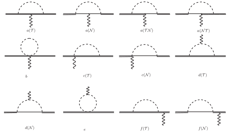
Figure 2: The one-loop diagrams where the decuplet (octet) baryon is denoted by the double (single) solid line. The dashed and wiggly lines represent the pseudoscalar meson and photon respectively. For the wave function renormalization in diagram f, only representative graphs are shown. We do not also list the adjoint graphs for diagram c.

There are twelve Feynman diagrams at one-loop level as shown in Fig. 2 and we divide them into six types (a-f) according to the structure. All the vertices in these diagrams come from Eqs. (17),(26-33). In diagram a, the meson vertex is from the strong interaction terms in Eq. (27) while the photon vertex from the $\mathcal{O}(p^{2})$ tree level magnetic moment interaction in Eqs. (29),(32),(33). In diagram b, the photon-meson-baryon vertex is also from the $\mathcal{O}(p^{2})$ tree level magnetic moment interaction in Eq. (29). In diagram c, the two vertices are from the strong interaction and seagull terms respectively. In diagram d, the meson vertex is from the strong interaction terms while the photon vertex is from the meson photon interaction term in Eq. (17). In diagram e, the meson-baryon vertex is from the second order pseudoscalar meson and baryon Lagrangian in Eq. (28) while the photon vertex is also from the meson photon interaction term. In diagram f, the meson vertex is from the strong interaction terms while the photon vertex from the $\mathcal{O}(p^{2})$ tree level magnetic moment interaction.

The diagrams a, b, e and f contribute to the tensor $e\mathcal{O}_{\rho\mu\sigma}$ at $\mathcal{O}(p^{4})$ while the diagram d contributes at $\mathcal{O}(p^{3})$. The diagram c vanishes in the heavy baryon mass limit. If the intermediate baryon is a decuplet (or octet) state, the amplitude of the diagram c is denoted as $J_{c(\mathcal{T})}$ (or $J_{c(\mathcal{N})}$). We have

$$J_{c(\mathcal{T})} \propto \int\frac{d^{d}l}{(2\pi)^{d}}\frac{i}{l^{2}-m^{2}_{\phi}+i\epsilon}\frac{g_{\mathcal{H}}(S\cdot l)}{f_{0}}\frac{-iP_{\rho\sigma}^{3/2}}{v\cdot l+i\epsilon}S_{\mu}$$

$$\propto S\cdot v=0,$$

$$J_{c(\mathcal{N})} \propto \int\frac{d^{d}l}{(2\pi)^{d}}\frac{i}{l^{2}-m^{2}_{\phi}+i\epsilon}\frac{g_{\mathcal{H}}l_{\sigma}}{f_{0}}\frac{i}{v\cdot l-\omega+i\epsilon}g_{\mu\rho}$$

$$\propto g_{\mu\rho}v_{\sigma},$$

where $P_{\rho\sigma}^{3/2}$ is the non-relativistic spin-$\frac{3}{2}$ projector. $J_{c(\mathcal{T})}$ vanishes, and $J_{c(\mathcal{N})}$ also vanishes since $v_{\sigma}u^{\sigma}=0$. In other words, this diagram does not contribute to the magnetic moments of the decuplet baryons in the leading order of the heavy baryon expansion.

For diagram c, there are two adjoint graphs in which the photon moves from the left vertex to the right one. There are also two adjoint graphs for diagram f. We include the contributions from the adjoint graphs in our results. We use diagram f to indicate the corrections from the renormalization of the external leg where Lehmann-Symanzik-Zimmermann reduction formula is used.

The leading-order loop contributions to the multipole form factors are

$$F^{(2,\rm loop)}_{1} = \sum_{\phi=\pi,K}\{\frac{\mathcal{H}^{2}\beta_{\mathcal{T}}^{\phi}}{f_{\phi}^{2}}[\frac{1}{4}q^{2}(2n^{{\rm I\!I}0}_{4\phi}+2n^{{\rm I\!I\!I}0}_{4\phi})+\frac{5}{6}n^{{\rm I\!I\!I}0}_{13\phi}+\frac{1}{3}(\frac{q^{2}}{2M_{T}})n^{{\rm I\!I}0}_{1\phi}]+\frac{\mathcal{C}^{2}\beta_{\mathcal{N}}^{\phi}}{4f_{\phi}^{2}}[2n^{{\rm I\!I\!I}}_{13\phi}+(-\frac{q^{2}}{2M_{T}})n^{{\rm I\!I}}_{1\phi}]\},$$ (47)

$$F^{(1,\rm loop)}_{2} = \sum_{\phi=\pi,K}\{\frac{\mathcal{H}^{2}\beta_{\mathcal{T}}^{\phi}}{f_{\phi}^{2}}[-\frac{M_{T}}{3}(1+\frac{q^{2}}{4M_{T}^{2}})]n^{{\rm I\!I}0}_{1\phi}+\frac{\mathcal{C}^{2}\beta_{\mathcal{N}}^{\phi}}{f_{\phi}^{2}}[-\frac{M_{T}}{2}(1-\frac{q^{2}}{4M_{T}^{2}})]n^{{\rm I\!I}}_{1\phi}\},$$ (48)

$$F^{(0,\rm loop)}_{3} = \sum_{\phi=\pi,K}\{\frac{\mathcal{H}^{2}\beta_{\mathcal{T}}^{\phi}}{f_{\phi}^{2}}\frac{-1}{3}[4M_{T}^{2}(2n^{{\rm I\!I}0}_{4\phi}+2n^{{\rm I\!I\!I}0}_{4\phi})+4M_{T}n^{{\rm I\!I}0}_{1\phi}]+\frac{\mathcal{C}^{2}\beta_{\mathcal{N}}^{\phi}}{4f_{\phi}^{2}}[4M_{T}^{2}(2n^{{\rm I\!I}}_{4\phi}+2n^{{\rm I\!I\!I}}_{4\phi})+4M_{T}n^{{\rm I\!I}}_{1\phi}]\},$$ (49)

$$F^{(-1,\rm loop)}_{4} = 0.$$ (50)

where $n^{{\rm I\!I}}_{1\phi},n^{{\rm I\!I}}_{4\phi},n^{{\rm I\!I\!I}}_{4\phi},n^{{\rm I\!I\!I}}_{13\phi}$ are $n^{{\rm I\!I}}_{1},n^{{\rm I\!I}}_{4},n^{{\rm I\!I\!I}}_{4},n^{{\rm I\!I\!I}}_{13}$, respectively, defined in the appendix A with $m=m_{\phi}$ and $\omega=\delta$. When $\omega=0$, they become $n^{{\rm I\!I}0}_{1\phi},n^{{\rm I\!I}0}_{4\phi},n^{{\rm I\!I\!I}0}_{4\phi},n^{{\rm I\!I\!I}0}_{13\phi}$. The coefficients $\beta^{\phi}_{\mathcal{T}}$ and $\beta^{\phi}_{\mathcal{N}}$ arise from the decuplet and octet intermediate states respectively. We use the number $n$ within the parenthesis in the superscript of $X^{(n,...)}$ to indicate the chiral order of $X$.

The tensor $e\mathcal{O}_{\rho\mu\sigma}$ at $\mathcal{O}(p^{3})$ should contribute to $F_{4}$ at $\mathcal{O}(p^{-1})$. However, such contribution is 0 from Eq. (50). Moreover, all the loop diagrams in Fig. 2 do not contribute to $F_{4}$ up to $\mathcal{O}(p^{0})$. Therefore, in our case $F_{4}=F_{4}^{(0,\rm tree)}\sim d_{\mathcal{O}}Q$. If one tries to obtain the next-to-leading order correction of $F_{4}$, $e\mathcal{O}_{\rho\mu\sigma}$ at $\mathcal{O}(p^{5})$ must be systematically considered.

Summing all the contributions in Fig. 2, the leading and next-to-leading order loop corrections to the decuplet magnetic moments can be expressed as

$$\mu_{\mathcal{T}}^{(2,\rm loop)} = \frac{e}{2M_{T}}\sum_{\phi=\pi,K}[-\frac{1}{3}\mathcal{H}^{2}M_{T}d_{\mathcal{T}}\frac{\beta_{\mathcal{T}}^{\phi}}{f_{\phi}^{2}}-\frac{1}{2}\mathcal{C}^{2}M_{T}\frac{\beta_{\mathcal{N}}^{\phi}}{f_{\phi}^{2}}d_{\mathcal{N}}],$$ (51)

$$\mu_{\mathcal{T}}^{(3,\rm loop)} = \frac{e}{2M_{T}}\left[\sum_{\phi=\pi,K}(\gamma_{b}^{\phi}+\gamma_{e}^{\phi})\frac{m_{\phi}^{2}}{8\pi^{2}f_{\phi}^{2}}\ln\frac{m_{\phi}}{{\lambda}}-\sum_{\phi=\pi,K,\eta}(\frac{2}{3f_{\phi}^{2}}\frac{5b\mathcal{H}^{2}}{12}a_{\mathcal{T}}\gamma_{a\mathcal{T}}^{\phi}+\frac{\mathcal{C}^{2}}{16f_{\phi}^{2}}a_{\mathcal{N}}\gamma_{a\mathcal{N}}^{\phi}-\frac{b_{2}\mathcal{C}\mathcal{H}}{3\delta f_{\phi}^{2}}a_{\mathcal{T}\mathcal{N}}\gamma^{\phi}_{a\mathcal{T}\mathcal{N}})\right]$$ (52)

$$+\sum_{\phi=\pi,K,\eta}(\frac{5\mathcal{H}^{2}}{12}\frac{\mu_{\mathcal{T}}^{(1)}}{f_{\phi}^{2}}a_{\mathcal{T}}\gamma_{f\mathcal{T}}^{\phi}-\frac{\mu_{\mathcal{T}}^{(1)}}{4f_{\phi}^{2}}\mathcal{C}^{2}a_{\mathcal{N}}\gamma_{f\mathcal{N}}^{\phi}),\quad$$

where ${\lambda}=1$ GeV is the renormalization scale. $\gamma^{\phi}_{a\mathcal{T}}$, $\gamma^{\phi}_{a\mathcal{N}}$, $\gamma^{\phi}_{a\mathcal{T}\mathcal{N}}$, $\gamma^{\phi}_{b}$, $\gamma^{\phi}_{e}$, $\gamma^{\phi}_{f\mathcal{T}}$ and $\gamma^{\phi}_{f\mathcal{N}}$ arise from the corresponding diagrams in Fig. 2. We collect their explicit expressions in Tables 5, 6, 7 in the Appendix B.

$$d_{\mathcal{T}} = \frac{m_{\phi}}{16\pi},$$ (53)

$$d_{\mathcal{N}} = \frac{1}{16\pi^{2}}\begin{cases}\displaystyle\delta\left(\log\frac{m_{\phi}^{2}}{{\lambda}^{2}}-1\right)-2\sqrt{\delta^{2}-m_{\phi}^{2}}\left({\rm arccosh}\left(\frac{-\delta}{m_{\phi}}\right)-i\pi\right)&\phi=\pi\\ \displaystyle\delta\left(\log\frac{m_{\phi}^{2}}{{\lambda}^{2}}-1\right)+2\sqrt{m_{\phi}^{2}-\delta^{2}}\arccos\left(-\frac{\delta}{m_{\phi}}\right)&\phi=K,\eta\end{cases},$$ (54)

$$a{}_{\mathcal{T}} = -\frac{m_{\phi}^{2}}{8\pi^{2}}\ln\frac{m_{\phi}}{{\lambda}},$$ (55)

$$a{}_{\mathcal{N}} = \frac{1}{16\pi^{2}}\begin{cases}\displaystyle\left(m_{\phi}^{2}-2\delta^{2}\right)\log\left(\frac{m_{\phi}^{2}}{{\lambda}^{2}}\right)+4\delta\sqrt{\delta^{2}-m_{\phi}^{2}}\left({\rm arccosh}\left(\frac{-\delta}{m_{\phi}}\right)-i\pi\right)+2\delta^{2}&\phi=\pi\\ \displaystyle\left(m_{\phi}^{2}-2\delta^{2}\right)\log\left(\frac{m_{\phi}^{2}}{{\lambda}^{2}}\right)-4\delta\sqrt{m_{\phi}^{2}-\delta^{2}}\arccos\left(-\frac{\delta}{m_{\phi}}\right)+2\delta^{2}&\phi=K,\eta\end{cases},$$ (56)

$$a_{\mathcal{T}\mathcal{N}} = \frac{1}{144\pi^{2}}\left[\left(6\delta^{3}-9m_{\phi}^{2}\delta\right)\log\left(\frac{m_{\phi}^{2}}{{\lambda}^{2}}\right)+2\left(3\pi m_{\phi}^{3}+6m_{\phi}^{2}\delta-5\delta^{3}\right)\right]$$ (57)

$$-\frac{1}{12\pi^{2}}\begin{cases}\displaystyle\left(\delta^{2}-m_{\phi}^{2}\right)^{3/2}\left({\rm arccosh}\left(\frac{-\delta}{m_{\phi}}\right)-i\pi\right)&\phi=\pi\\ \displaystyle\left(m_{\phi}^{2}-\delta^{2}\right)^{3/2}\arccos\left(-\frac{\delta}{m_{\phi}}\right)&\phi=K,\eta\end{cases}.$$

With the low energy counter terms and loop contributions (51, 52), we obtain the magnetic moments,

$$\mu_{\mathcal{T}}=\left\{\mu_{\mathcal{T}}^{(1)}\right\}+\left\{\mu_{\mathcal{T}}^{(2,\rm loop)}\right\}+\left\{\mu_{\mathcal{T}}^{(3,\rm tree)}+\mu_{\mathcal{T}}^{(3,\rm loop)}\right\}$$ (58)

where $\mu_{\mathcal{T}}^{(1)}$ and $\mu_{\mathcal{T}}^{(3,\rm tree)}$ is the tree-level magnetic moments as shown in Table 1.

IV.2 The electromagnetic form factors and the radii

From the tensor $e\mathcal{O}_{\rho\mu\sigma}$ up to $\mathcal{O}(p^{4})$, the magnetic dipole form factor with the corrections at the next-to-next-leading order is

$$G_{M1}(q^{2})=\left\{F_{2}^{(0)}\right\}+\left\{F^{(1,\rm loop)}_{2}-F^{(\rm rec,loop)}_{2}\right\}+\left\{Q\tilde{b}_{q^{2}}q^{2}+F_{2}^{(2)}+F^{(\rm rec,loop)}_{2}\right\},$$ (59)

where the terms in the first, second, and the third curly braces are $G_{M1}$ at the leading, next-to-leading, and next-to-next-leading order, respectively. Here $F_{2}^{(0)}=2M_{T}\mu_{\mathcal{T}}^{(1)}/e$, $F_{2}^{(2)}=2M_{T}(\mu_{\mathcal{T}}^{(3,\rm tree)}+\mu_{\mathcal{T}}^{(3,\rm loop)})/e$, and

$$F^{(\rm rec,loop)}_{2}=-\frac{q^{2}}{4M_{T}}\sum_{\phi=\pi,K}(\frac{\mathcal{H}^{2}\beta_{\mathcal{T}}^{\phi}}{3f_{\phi}^{2}}n^{{\rm I\!I}0}_{1\phi}-\frac{\mathcal{C}^{2}\beta_{\mathcal{N}}^{\phi}}{2f_{\phi}^{2}}n^{{\rm I\!I}}_{1\phi}).$$ (60)

The other multipole form factors are

$$G_{E0}(q^{2}) = \left\{Q\right\}+\left\{Q\tilde{c}_{r}q^{2}+F^{(2,\rm loop)}_{1}-\frac{1}{3}\tau F^{(0,\rm loop)}_{3}\right\},$$ (61)

$$G_{E2}(q^{2}) = \left\{Q\tilde{c}_{\mathbb{Q}}-\frac{1}{2}F^{(0,\rm loop)}_{3}\right\},$$ (62)

$$G_{M3}(q^{2}) = Q\tilde{d}_{\mathcal{O}}.$$ (63)

where $\tilde{b}_{q^{2}}$, $\tilde{c}_{r}$, $\tilde{c}_{\mathbb{Q}}$, and $\tilde{d}_{\mathcal{O}}$ are the linear combinations of LECs $b$, $b_{q^{2}}$, $c_{r}$, $c_{\mathbb{Q}}$, and $d_{\mathcal{O}}$. We can estimate the LECs $\tilde{b}_{q^{2}}$ and $\tilde{c}_{r}$ with the SU(3) VMD model as shown in Section V.1. However, the LECs $\tilde{c}_{\mathbb{Q}}$ and $\tilde{d}_{\mathcal{O}}$ are still unknown for the electro quadrupole and magnetic octupole form factors. Hence we do not list the loop corrections to these multipole form factors at higher order.

The charge and magnetic radii of the decuplet baryons can be expressed as

$$\langle{r_{E}^{2}}\rangle = 6\frac{dG_{E0}(q^{2})}{dq^{2}}\mid_{q^{2}=0}=\langle{r_{E}^{2}}\rangle^{\rm tree}+\langle{r_{E}^{2}}\rangle^{\rm loop}=[6Q\tilde{c}_{r}]+6[\frac{dF^{(2,\rm loop)}_{1}}{dq^{2}}\mid_{q^{2}=0}+\frac{1}{12M_{T}^{2}}F^{(0,\rm loop)}_{3}(0)],$$ (64)

$$\langle{r_{M}^{2}}\rangle = \frac{6}{G_{M1}(0)}\frac{dG_{M1}(q^{2})}{dq^{2}}=\langle{r_{M}^{2}}\rangle^{\rm tree}+\langle{r_{M}^{2}}\rangle^{\rm loop}=\frac{6}{G_{M1}(0)}Q\tilde{b}_{q^{2}}+\frac{6}{G_{M1}(0)}\frac{dF^{(1,\rm loop)}_{2}}{dq^{2}}\mid_{q^{2}=0}.$$ (65)

For the neutral decuplet baryons, we normalize the magnetic radii as

$$\langle{r_{M}^{2}}\rangle = 6\frac{dG_{M1}(q^{2})}{dq^{2}}.$$ (66)

V Estimation of the low energy constants

V.1 The vector meson dominance model and estimation of some LECs

To calculate the tree level charge radii and magnetic radii, we can use the vector meson dominance (VMD) model to estimate the short-distance contribution.

Figure 3: The contribution to tree level charge radii from the vector meson dominance model. The double-solid, the double-dashed and wiggly lines represent the decuplet baryons, the vector meson and photon respectively.

It is well-known that the charge radii of the proton and pion are dominated by the short-distance contribution, which can be estimated very well by the VMD model. In this work, we use this model to estimate the LECs $\tilde{c}_{r}$ and $\tilde{b}_{q^{2}}$ which are related to the charge and magnetic radii of the decuplet baryons, respectively. Within this framework, the virtual photon transforms into a virtual vector meson which couples to the decuplet baryons as shown in Fig. 3.

It is convenient to adopt the antisymmetric Lorentz tensor field formulation for the vector meson Ecker:1988te ; Borasoy:1995ds , which has six degrees of freedom. But we can dispose of three of them in a systematic way. For details see Ref. Ecker:1988te . The kinetic and mass term of the effective Lagrangian for the vector meson has the form Ecker:1988te ; Borasoy:1995ds

$$\mathcal{L}_{0W}=-\frac{1}{2}{\rm Tr}(\partial^{\mu}W_{\mu\nu}\partial_{\sigma}W^{\sigma\nu})+\frac{1}{4}{\rm Tr}(M_{V}^{2}W_{\mu\nu}W^{\mu\nu}),$$ (67)

where

$$W_{\mu\nu}=\left(\begin{array}[]{ccc}\frac{\rho^{0}}{\sqrt{2}}+\frac{\omega}{\sqrt{2}}&\rho^{+}&K^{*+}\\ \rho^{-}&-\frac{\rho^{0}}{\sqrt{2}}+\frac{\omega}{\sqrt{2}}&K^{*0}\\ K^{*-}&\bar{K}^{*0}&\phi\end{array}\right)_{\mu\nu}.$$ (68)

The QED gauge-invariant interaction between the photon and vector meson can be written as

$$\mathcal{L}_{W}^{(2)}=\frac{f_{V}}{2\sqrt{2}}{\rm Tr}(W^{\mu\nu}F_{\mu\nu}^{+}).$$ (69)

The vector meson and decuplet baryon interaction Lagrangian reads

$$\mathcal{L}_{W\mathcal{T}}^{(1)}=g_{V\mathcal{T}}{\rm Tr}[\bar{T}^{\alpha}(\frac{1}{M_{V}}\gamma^{\mu}\nabla^{\nu}W_{\mu\nu}-\frac{\kappa}{2}\sigma^{\mu\nu}W_{\mu\nu})T_{\alpha}].$$ (70)

Under the SU(3) symmetry, the charge form factor and charge radii of the decuplet baryons are

$$G^{\rm VMD}_{E0}(q^{2}) = Q\frac{g_{V\mathcal{T}}f_{V}}{\sqrt{2}M_{V}}\frac{q^{2}}{-q^{2}+M_{V}^{2}},$$ (71)

$$\langle r_{E}^{2}\rangle^{\rm tree} \approx \langle r_{E}^{2}\rangle^{\rm VMD}=6\frac{dG^{\rm VMD}_{E0}(q^{2})}{dq^{2}}|_{q^{2}=0}=6Q\frac{g_{V\mathcal{T}}f_{V}}{\sqrt{2}}\frac{1}{M_{V}^{3}}.$$ (72)

The magnetic-dipole form factor and magnetic radii of the decuplet baryons are

$$G^{\rm VMD}_{M1}(q^{2}) = Q\frac{g_{V\mathcal{T}}f_{V}}{\sqrt{2}M_{V}}\frac{q^{2}}{-q^{2}+M_{V}^{2}}-\sqrt{2}\kappa Qg_{V\mathcal{T}}f_{V}\frac{M_{T}}{-q^{2}+M_{V}^{2}},$$ (73)

$$\langle r_{M}^{2}\rangle^{\rm tree} \approx \langle r_{M}^{2}\rangle^{\rm VMD}=\frac{6}{G_{M1}(0)}\frac{dG^{\rm VMD}_{M1}(q^{2})}{dq^{2}}|_{q^{2}=0}=\frac{6Q}{G_{M1}(0)}[\frac{g_{V\mathcal{T}}f_{V}}{\sqrt{2}M_{V}^{3}}+\frac{G^{\rm VMD}_{M1}(0)}{M_{V}^{2}Q}].$$ (74)

Now the LECs $\tilde{c}_{r}$ and $\tilde{b}_{q^{2}}$ read

$$\tilde{c}_{r} = \frac{g_{V\mathcal{T}}f_{V}}{\sqrt{2}M_{V}^{3}},$$ (75)

$$\tilde{b}_{q^{2}} = \frac{g_{V\mathcal{T}}f_{V}}{\sqrt{2}M_{V}^{3}}+\frac{G^{\rm tree}_{M1}(0)}{M_{V}^{2}Q}.$$ (76)

In the numerical analysis, we use $M_{\rho}=770.0\pm 0.3$ MeV, $f_{\rho}=f_{V}=152.5\pm 16.5$ MeV, $g_{V\mathcal{T}}\approx g_{\rho\mathcal{N}}=4.0\pm 0.4$ Kubis:2000zd , where we have considered the quark model error around 10% in Section V.2.

V.2 Quark model and estimation of some couplings

Comparing the matrix elements at both the hadron and quark level, one can express the couplings in terms of the constituent quark masses and/or other known hadron couplings. To estimate $g_{V\mathcal{T}}$, we first consider the $\Delta^{+}\Delta^{+}\rho^{0}$ and $pp\rho^{0}$ vertices at the hadron level,

$$\mathcal{L}_{\Delta^{+}\Delta^{+}\rho^{0}} = \frac{g_{V\mathcal{T}}}{\sqrt{2}M_{V}}{\bar{\Delta^{+}}}^{\alpha}\gamma^{\mu}\partial^{\nu}\rho^{0}_{\mu\nu}\Delta^{+}_{\alpha},$$ (77)

$$\mathcal{L}_{pp\rho^{0}} = \frac{g_{\rho\mathcal{N}}}{\sqrt{2}M_{V}}{\bar{p}}\gamma^{\mu}\partial^{\nu}\rho^{0}_{\mu\nu}p.$$ (78)

At the quark level, the quark vector meson interaction reads

$$\mathcal{L}_{qq\rho^{0}}=g_{qq\rho}\bar{q}_{a}\gamma^{\mu}\partial^{\nu}\rho^{0}_{\mu\nu}q_{a}.$$ (79)

With the help of the flavor wave functions of the static $\Delta^{+}$ and $p$ states, we obtain the matrix elements at the hadron level

$$\langle\Delta^{+}\mid i\mathcal{L}_{\Delta^{+}\Delta^{+}\rho^{0}}\mid\Delta^{+};\rho^{0}\rangle = \frac{g_{V\mathcal{T}}}{\sqrt{2}M_{V}}2m_{\Delta^{+}}q_{\rho}^{\mu}\epsilon_{\mu 0},$$ (80)

$$\langle p\mid i\mathcal{L}_{pp\rho^{0}}\mid p;\rho^{0}\rangle = \frac{g_{\rho\mathcal{N}}}{\sqrt{2}M_{V}}2m_{p}q_{\rho}^{\mu}\epsilon_{\mu 0},$$ (81)

and at the quark level,

$$\langle\Delta^{+}\mid i\mathcal{L}_{qq\rho^{0}}\mid\Delta^{+};\rho^{0}\rangle = 2g_{qq\rho}(2m_{u}+m_{d})q_{\rho}^{\mu}\epsilon_{\mu 0},$$ (82)

$$\langle p\mid i\mathcal{L}_{qq\rho^{0}}\mid p;\rho^{0}\rangle = 2g_{qq\rho}(2m_{u}+m_{d})q_{\rho}^{\mu}\epsilon_{\mu 0},$$ (83)

Comparing the hadron and quark level matrix element and neglecting the mass difference between $p$ and $\Delta^{+}$, we finally obtain

$$g_{V\mathcal{T}}=g_{\rho\mathcal{N}}.$$ (84)

In the same way, one can estimate the LEC $b_{2}$ by comparing $\Sigma^{*0}\rightarrow\Lambda+\gamma$ matrix element at both the hadron and quark level with the Lagrangians

$$\mathcal{L}^{(2)}_{\Sigma^{*0}\rightarrow\Lambda+\gamma}=-\frac{b_{2}}{4M_{B}}{\bar{\Sigma}^{*0\mu}}\gamma^{\nu}\gamma_{5}\Lambda F_{\mu\nu},$$ (85)

and

$$\mathcal{L}_{\rm Im}=-\frac{e}{4}(\frac{2}{3m_{u}}\bar{u}\sigma^{\mu\nu}u-\frac{1}{3m_{d}}\bar{d}\sigma^{\mu\nu}d-\frac{1}{3m_{s}}\bar{s}\sigma^{\mu\nu}s)F_{\mu\nu}.$$ (86)

We obtain

$$b_{2}=4M_{B}\sqrt{\frac{3}{2}}(\frac{1}{3\sqrt{6}m_{u}}+\frac{1}{6\sqrt{6}m_{d}})=3.45\pm 0.35.$$ (87)

with $m_{u}=m_{d}=336\pm 34~{}{\rm MeV}$ Scadron:2006dy , where we have considered the quark model error around 10%.

VI NUMERICAL RESULTS AND DISCUSSIONS

baryons	$\mathcal{O}(p^{1})$ tree	$\mathcal{O}(p^{2})$ loop	$\mathcal{O}(p^{3})$ tree	$\mathcal{O}(p^{3})$ loop	total
$\Delta^{++}$	$\frac{4}{3}b$	$-3.54$	$-\frac{2}{3}d_{1}$	$0.49-0.50b-0.02b_{D}-0.07b_{F}-0.36g_{2}$	4.97(89)
$\Delta^{+}$	$\frac{2}{3}b$	$-1.91$	$-\frac{2}{3}d_{1}$	$0.22-0.21b-0.01b_{D}-0.04b_{F}-0.27g_{2}$	2.60(50)
$\Delta^{0}$	0	$-0.29$	$-\frac{2}{3}d_{1}$	$-0.27+0.06b+0.001b_{D}-0.001b_{F}-0.18g_{2}$	0.02(12)
$\Delta^{-}$	$-\frac{2}{3}b$	$1.34$	$-\frac{2}{3}d_{1}$	$-0.32+0.20b+0.01b_{D}+0.02b_{F}-0.14g_{2}$	-2.48(32)
$\Sigma^{*+}$	$\frac{2}{3}b$	$-1.63$	$-\frac{2}{3}d_{1}-\frac{2}{9}d_{2}+\frac{4}{9}d_{3}$	$0.17-0.50b-0.001b_{D}-0.04b_{F}-0.33g_{2}$	1.76(38)
$\Sigma^{*0}$	$0$	$0$	$-\frac{2}{3}d_{1}-\frac{2}{9}d_{2}+\frac{1}{9}d_{3}$	$-0.02-0.001b_{D}-0.24g_{2}$	-0.02(3)
$\Sigma^{*-}$	$-\frac{2}{3}b$	$1.63$	$-\frac{2}{3}d_{1}-\frac{2}{9}d_{2}-\frac{2}{9}d_{3}$	$-0.27+0.50b-0.001b_{D}+0.04b_{F}-0.15g_{2}$	-1.85(38)
$\Xi^{*0}$	$0$	$0.29$	$-\frac{2}{3}d_{1}-\frac{4}{9}d_{2}+\frac{2}{9}d_{3}$	$-0.21-0.06b+0.01b_{D}+0.001b_{F}-0.30g_{2}$	-0.42(13)
$\Xi^{*-}$	$-\frac{2}{3}b$	$1.91$	$-\frac{2}{3}d_{1}-\frac{4}{9}d_{2}-\frac{4}{9}d_{3}$	$-0.22+0.60b-0.001b_{D}+0.04b_{F}-0.21g_{2}$	-1.90(47)
$\Omega^{-}$	$-\frac{2}{3}b$	$2.20$	$-\frac{2}{3}d_{1}-\frac{2}{3}d_{2}-\frac{2}{3}d_{3}$	$0.17+0.65b+0.01b_{D}+0.02b_{F}-0.27g_{2}$	-2.02(5)

Table 1: The magnetic moments of the decuplet baryons to the next-to-next-leading order (in unit of $\mu_{N}$).

baryons	$\mathcal{O}(p^{1})$	$\mathcal{O}(p^{2})$	$\mathcal{O}(p^{3})$	PDG
$\Delta^{++}$	$4.04(10)$	$4.90(84)$	4.97(89)	5.6±1.9
$\Delta^{+}$	$2.02(5)$	$2.31(47)$	2.60(50)	2.7 ± 3.5
$\Delta^{0}$	0	$-0.29(11)$	0.02(12)
$\Delta^{-}$	$-2.02(5)$	$-2.88(27)$	-2.48(32)
$\Sigma^{*+}$	$2.02(5)$	$2.59(37)$	1.76(38)
$\Sigma^{*0}$	$0$	$0$	-0.02(3)
$\Sigma^{*-}$	$-2.02(5)$	$-2.59(37)$	-1.85(38)
$\Xi^{*0}$	$0$	$0.29(11)$	-0.42(13)
$\Xi^{*-}$	$-2.02(5)$	$-2.31(47)$	-1.90(47)
$\Omega^{-}$	$-2.02(5)$	$-2.02(5)$	-2.02(5)	-2.02 ±0.05

Table 2: The magnetic moments of the decuplet baryons when the chiral expansion is truncated at $\mathcal{O}(p^{1})$, $\mathcal{O}(p^{2})$ and $\mathcal{O}(p^{3})$ respectively (in unit of $\mu_{N}$).

We collect our numerical results of the magnetic moments of the decuplet baryons to the next-to-next-leading order in Table 1. We also compare the numerical results of the magnetic moments when the chiral expansion is truncated at orders $\mathcal{O}(p^{1})$, $\mathcal{O}(p^{2})$ and $\mathcal{O}(p^{3})$ respectively in Table 2.

At the leading order $\mathcal{O}(p^{1})$, there is only one unknown low energy constant $b$. We use the precise experimental measurement of the $\Omega^{-}$ magnetic moment $\mu_{\Omega^{-}}=(-2.02\pm 0.05)\mu_{N}$ as input to extract $b=3.03\pm 0.08$. The magnetic moments of the other decuplet baryons are given in the second column in Table 2. Notice that the $\mathcal{O}(p^{1})$ tree level magnetic moments of the neutral baryons $\Delta^{0}$, $\Sigma^{*0}$ and $\Xi^{*0}$ vanish. In the limit of the exact SU(3) flavor symmetry, there exits only one independent term for the magnetic interaction in the $\mathcal{O}(p^{2})$ Lagrangian of the decuplet baryons due to the constraint of the decuplet flavor structure. Therefore, the leading order $\mathcal{O}(p^{1})$ magnetic moments of the decuplet baryons are proportional to their charge, which is in strong contrast with the case of the octet baryons. The magnetic moments of the neutral octet baryons do not vanish at the leading order because there exist two independent magnetic interaction terms as illustrated in Refs. Jenkins:1992pi ; Meissner:1997hn .

Up to $\mathcal{O}(p^{2})$, we need include both the leading tree-level magnetic moments and the $\mathcal{O}(p^{2})$ loop corrections. At this order, all the coupling constants are well-known. There do not exist new LECs. Again, we use the experimental value of the $\Omega^{-}$ magnetic moment $\mu_{\Omega^{-}}=(-2.02\pm 0.05)\mu_{N}$ as input to extract the LEC $b=6.3\pm 0.1$. We list the numerical results in the third column in Table 2, where the errors in the brackets are dominated by the errors of the coupling constants $\mathcal{C},\mathcal{H}$ in Eq. (27).

It’s interesting to notice that the magnetic moment of $\Sigma^{*0}$ still vanishes even at $\mathcal{O}(p^{2})$. The reason is as follows. Throughout our calculation, we neglect the mass difference among different decuplet baryons in the loop and have used the same propagator $\frac{-iP_{\rho\sigma}^{3/2}}{v\cdot q+i\epsilon}$ for all the decuplet baryons. In the case of the $\Sigma^{*0}$ magnetic moment, the loop contributions from different intermediate states cancel each other. I.e., the pion loop contributions with the intermediate baryons $\Sigma^{*+}$ and $\Sigma^{*-}$, $\Sigma^{+}$ and $\Sigma^{-}$ cancel each other due to the exact SU(2) flavor symmetry. The kaon loop contributions with the intermediate baryons $\Delta^{+}$ and $\Xi^{*-}$, $p$ and $\Xi^{-}$ cancel each other due to the SU(3) flavor symmetry. Hence, the magnetic moment of $\Sigma^{*0}$ is zero to $\mathcal{O}(p^{2})$ in Table 2.

Up to $\mathcal{O}(p^{3})$, there are seven unknown LECs: $b_{D,F}$, $b$, $g_{2}$, $d_{1,2,3}$. The first two LECs were extracted in the calculation of the magnetic moments of the octet baryons in Ref. Meissner:1997hn : $b_{D}=3.9$, $b_{F}=3.0$. We use the experimental value of the $\Omega^{-}$ magnetic moment, the magnetic moments of the $\Delta$ baryons in Ref. Cloet:2003jm ($\mu_{\Delta^{++}}=4.99\pm 0.56,\mu_{\Delta^{+}}=2.49\pm 0.27,\mu_{\Delta^{0}}=0.06\pm 0.00,\mu_{\Delta^{-}}=-2.45\pm 0.27$) and $\mu_{\Sigma^{*0}}=0$ to extract the remaining five LECs: $b=6.8\pm 0.4$, $g_{2}=-13.7\pm 0.1$, $d_{1}=3.5\pm 0.1$, $d_{2}=-1.5\pm 0.1$, $d_{3}=4.3\pm 0.1$. We list the numerical results up to $\mathcal{O}(p^{3})$ in the fourth column in Table 2 after taking the uncertainties of these inputs into consideration. In the error analysis, we use the least $\chi^{2}$ fitting tool of the TMinuit software package to get the errors of fitting. To get the total errors of the $\mathcal{O}(p^{3})$ magnetic moments, we have considered the errors of the coupling constants $\mathcal{C},\mathcal{H}$, the error of coupling constant $b_{2}$ and the errors of fitting.

In order to study the convergence of the chiral expansion, we show the numerical results at each order for the decuplet magnetic moment:

$$\mu_{\Delta^{++}} = 9.0(1-0.39-0.06)=4.97,$$

$$\mu_{\Delta^{+}} = 4.5(1-0.43+0.01)=2.60,$$

$$\mu_{\Delta^{0}} = -0.29(0+1-1.06)=0.02,$$

$$\mu_{\Delta^{-}} = -4.5(1-0.30-0.15)=-2.48,$$

$$\mu_{\Sigma^{*+}} = 4.5(1-0.36-0.25)=1.76,$$

$$\mu_{\Sigma^{*0}} = 0+0-0.02,$$

$$\mu_{\Sigma^{*-}} = -4.5(1-0.36-0.23)=-1.85,$$

$$\mu_{\Xi^{*0}} = 0.29(0+1-2.44)=-0.42,$$

$$\mu_{\Xi^{*-}} = -4.5(1-0.43-0.15)=-1.90,$$

$$\mu_{\Omega^{-}} = -4.5(1-0.49-0.06)=-2.02.$$ (88)

For the neutral decuplet baryons, their magnetic moments vanish at $\mathcal{O}(p^{1})$. Their total magnetic moments arise from the loop contributions at $\mathcal{O}(p^{2,3})$ and the tree-level LECs $d_{1,2,3}$ at $\mathcal{O}(p^{3})$ which are related to the strange quark mass correction. For the charged baryons, one observes rather good convergence of the chiral expansion and the leading order term dominates in these channels.

In order to illustrate the variation of the multipole form factors with the photon momentum $q$, we show the $\tilde{q}^{2}=-q^{2}$ dependence of the electric charge and magnetic dipole form factors to $\mathcal{O}(p^{3})$ in Figs. 4-5, where we have used the SU(3) VMD model to estimate the LEC $b_{q^{2}}$ and $c_{r}$ as shown in Eqs. (29),(34).

In Fig. 4 or Fig. 5, we notice that there is not much difference between the slopes of the curves. They should be exactly the same for different decuplet baryons if only the tree-level contributions are considered. The difference arises from the loop correction.

The electric quadrupole form factors $G_{E2}(q^{2})$ contain interesting information on the deformation of decuplet baryons. $\tilde{c}_{\mathbb{Q}}$ cannot be determined because of the lack of experimental data. But the $\tilde{c}_{\mathbb{Q}}$ term does not change with $q^{2}$. We list the normalized $F^{(0,\rm loop)}_{3}(-\tilde{q}^{2})$ in Fig. 6 to indicate the variation of $G_{E2}(q^{2})$.

In Table 3 we show numerical results for the charge radii and magnetic radii of the decuplet baryons. One can check that the charge radii estimated from the VMD model are proportional to the charge $Q$ of the decuplet baryons, while the magnetic radii estimated from the VMD model are the same for different baryons. In the error analysis, the errors of VMD radii are dominated by the input parameters $M_{\rho},f_{V},g_{V\mathcal{T}}$ and their propagation. The chiral correction radii are dominated by the errors of the coupling constants $\mathcal{C},\mathcal{H}$ in Eq. (27).

$\langle r_{E}^{2}\rangle/\rm fm^{2}$	VMD	chiral correction	total value	$\langle r_{M}^{2}\rangle/\rm fm^{2}$	VMD	chiral correction	total value
$\Delta^{++}$	0.44(20)	0.16(6)	0.60(21)	$\Delta^{++}$	0.46(11)	0.15(10)	0.61(15)
$\Delta^{+}$	0.22(10)	0.07(3)	0.29(10)	$\Delta^{+}$	0.46(11)	0.18(8)	0.64(14)
$\Delta^{0}$	0	-0.02(1)	-0.02(1)	$\Delta^{0}$	0	0.07(12)	0.07(12)
$\Delta^{-}$	-0.22(10)	-0.11(5)	-0.33(11)	$\Delta^{-}$	0.46(11)	0.09(15)	0.55(19)
$\Sigma^{*+}$	0.22(10)	0.09(4)	0.31(11)	$\Sigma^{*+}$	0.46(11)	0.13(12)	0.59(16)
$\Sigma^{*0}$	0	0	0	$\Sigma^{*0}$	0	0	0
$\Sigma^{*-}$	-0.22(10)	-0.09(4)	-0.31(11)	$\Sigma^{*-}$	0.46(11)	0.13(12)	0.59(16)
$\Xi^{*0}$	0	0.02(1)	0.02(1)	$\Xi^{*0}$	0	-0.07(12)	-0.07(12)
$\Xi^{*-}$	-0.22(10)	-0.07(3)	-0.29(10)	$\Xi^{*-}$	0.46(11)	0.18(8)	0.64(14)
$\Omega^{-}$	-0.22(10)	-0.05(2)	-0.27(10)	$\Omega^{-}$	0.46(11)	0.24(4)	0.70(12)

Table 3: Charge radii and magnetic radii (in ${\rm fm^{2}}$).

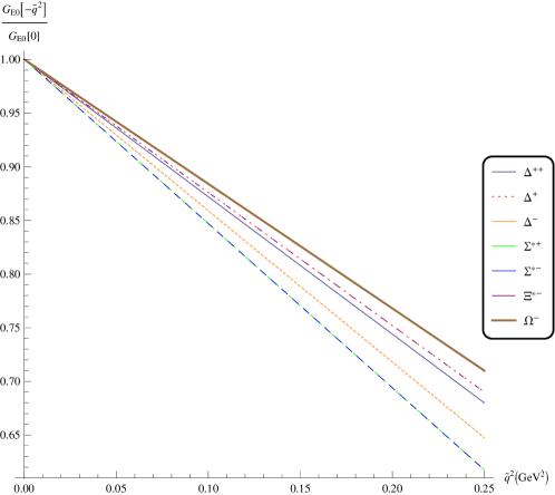
Figure 4: The variation of the normalized electric charge form factor $G_{E0}(-\tilde{q}^{2})$ with $\tilde{q}^{2}=-q^{2}>0$.

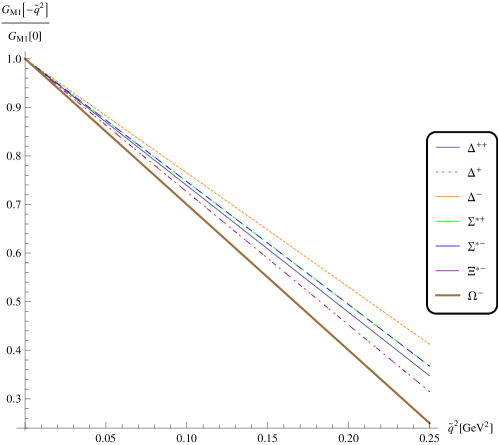
Figure 5: The variations of ${G_{M1}(-\tilde{q}^{2})\over G_{M1}(0)}$ with $\tilde{q}^{2}$.

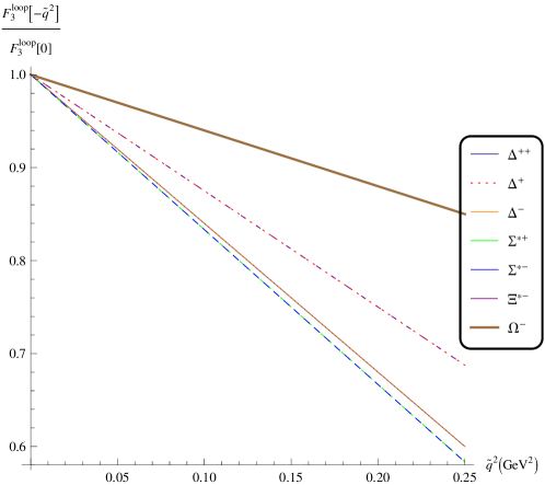
Figure 6: The variations of ${F^{(0,\rm loop)}_{3}(-\tilde{q}^{2})\over F^{(0,\rm loop)}_{3}(0)}$ with $\tilde{q}^{2}$.

VII Conclusions

In short summary, we have systematically studied the magnetic moments of the decuplet baryons up to the next-to-next-leading order in the framework of the heavy baryon chiral perturbation theory. With both the octet and decuplet baryon intermediate states in the chiral loops, we have systematically calculated the chiral corrections to the magnetic moments of the decuplet baryons order by order. The chiral expansion converges rather well for the charged channels. In Table 4, we compare our results obtained in the HBChPT with those from other model calculations such as lattice QCD Leinweber:1992hy , chiral quark model Wagner:2000ii , non relativistic quark model Hikasa:1992je , QCD sum rules  Lee:1997jk , large $N_{c}$ Luty:1994ub , covariant ChPT Geng:2009ys and next-to-leading order HBChPT Butler:1993ej . We also list the experimental values in the PDG Agashe:2014kda . One may observe the qualitatively similar features for the magnetic moments of the decuplet baryons.

Because of the SU(3) flavor symmetry, there is one independent low energy constant at the leading order. Hence, the magnetic moments of the decuplet baryons are proportional to their charge. Therefore, the magnetic moments of the neutral decuplet baryons vanish at $\mathcal{O}(p^{1})$, which differs from the case of the neutral octet baryons. There exist two independent magnetic interaction terms for the octet baryons, which ensures a large magnetic moment for the neutron at the leading order.

For the magnetic moment of the $\Sigma^{*0}$, the pion loop contributions with the $\Sigma^{*+}$ and $\Sigma^{*-}$, $\Sigma^{+}$ and $\Sigma^{-}$ intermediate states cancel each other exactly in the SU(2) symmetry limit. The kaon loop contributions with the $\Delta^{+}$ and $\Xi^{*-}$, $p$ and $\Xi^{-}$ intermediate states cancel each other exactly in the SU(3) symmetry limit. The magnetic moment of $\Sigma^{*0}$ vanishes even at $\mathcal{O}(p^{2})$ with SU(3) symmetry. The non-vanishing SU(3) breaking corrections first appear at $\mathcal{O}(p^{3})$. In other words, the SU(3) flavor symmetry demands that the magnetic moment of $\Sigma^{*0}$ be significantly smaller than those of the charged decuplet baryons.

We hope that the magnetic moments of the decuplet baryons will be measured experimentally in future experiments. Moreover, the analytical expressions derived in this work may be useful to the possible chiral extrapolation of the lattice simulations of the decuplet electromagnetic properties in the coming future.

baryons	$\Delta^{++}$	$\Delta^{+}$	$\Delta^{0}$	$\Delta^{-}$	$\Sigma^{*+}$	$\Sigma^{*0}$	$\Sigma^{*-}$	$\Xi^{*0}$	$\Xi^{*-}$	$\Omega^{-}$
LQCD Leinweber:1992hy	6.09	3.05	0	-3.05	3.16	0.329	-2.50	0.58	-2.08	-1.73
ChQM Wagner:2000ii	6.93	3.47	0	-3.47	4.12	0.53	-3.06	1.10	-2.61	-2.13
NQM Hikasa:1992je	5.56	2.73	-0.09	-2.92	3.09	0.27	-2.56	0.63	-2.2	-1.84
QCD-SR Lee:1997jk	4.1	2.07	0	-2.07	2.13	-0.32	-1.66	-0.69	-1.51	-1.49
large $N_{c}$ Luty:1994ub	5.9	2.9	—	-2.9	3.3	0.3	-2.8	0.65	-2.30	-1.94
covariant ChPT Geng:2009ys	6.04	2.84	-0.36	-3.56	3.07	0	-3.07	0.36	-2.56	-2.02
HBChPT Butler:1993ej	4.0	2.1	-0.17	-2.25	2.0	-0.07	-2.2	0.10	-2.0	-1.94
PDG Agashe:2014kda	5.6±1.9	2.7 $\pm$ 3.5	—	—	—	—	—	—	—	-2.02 $\pm$0.05
this work	4.97(89)	2.60(50)	0.02(12)	-2.48(32)	1.76(38)	-0.02(3)	-1.85(38)	-0.42(13)	-1.90(47)	-2.02(5)

Table 4: Comparison of the magnetic moments of the decuplet baryons in literature including lattice QCD(LQCD) Leinweber:1992hy , chiral quark model(ChQM) Wagner:2000ii , non relativistic quark model(NQM) Hikasa:1992je , QCD sum rules(QCD-SR) Lee:1997jk , large $N_{c}$ Luty:1994ub , covariant ChPT Geng:2009ys , next-to-leading order HBChPT Butler:1993ej and PDG Agashe:2014kda (in unit of $\mu_{N}$).

Appendix A Integrals and loop functions

We collect some common integrals and loop functions in this appendix.

A.1 The integrals with one or two meson propagators

$$\Delta = i\int\frac{d^{d}l\,{\lambda}^{4-d}}{(2\pi)^{d}}\frac{1}{l^{2}-m^{2}}=2m^{2}(L({\lambda})+\frac{1}{32\pi^{2}}\ln\frac{m^{2}}{{\lambda}^{2}}),$$ (89)

$$L({\lambda}) = \frac{{\lambda}^{d-4}}{16\pi^{2}}[\frac{1}{d-4}-\frac{1}{2}(\ln 4\pi+1+\Gamma^{\prime}(1))].$$ (90)

$$I_{0}(q^{2}) = i\int\frac{d^{d}l\,{\lambda}^{4-d}}{(2\pi)^{d}}\frac{1}{(l^{2}-m^{2}+i\epsilon)((l+q)^{2}-m^{2}+i\epsilon)}$$ (91)

$$= \begin{cases}\displaystyle-\frac{1}{16\pi^{2}}(1-\ln\frac{m^{2}}{{\lambda}^{2}}-r\ln|\frac{1+r}{1-r}|)+2L({\lambda})&\left(q^{2}<0\right)\\ \displaystyle-\frac{1}{16\pi^{2}}(1-\ln\frac{m^{2}}{{\lambda}^{2}}-2r\,\arctan\frac{1}{r})+2L({\lambda})&(0<q^{2}<4m^{2})\\ \displaystyle-\frac{1}{16\pi^{2}}(1-\ln\frac{m^{2}}{{\lambda}^{2}}-r\ln|\frac{1+r}{1-r}|+i\pi r)+2L({\lambda})&(q^{2}>4m^{2})\end{cases},$$

where $r=\sqrt{|1-4m^{2}/q^{2}|}$.

A.2 The integrals with one baryon propagator and one meson propagator

$$i\int\frac{d^{d}l\,{\lambda}^{4-d}}{(2\pi)^{d}}\frac{[1,l_{\alpha},l_{\alpha}l_{\beta}]}{(l^{2}-m^{2}+i\epsilon)(\omega+v\cdot l+i\epsilon)}=[J_{0}(\omega),v_{\alpha}J_{1}(\omega),g_{\alpha\beta}J_{2}(\omega)+v_{\alpha}v_{\beta}J_{3}(\omega)],\omega=v\cdot r+\delta$$ (92)

$$J_{0}(\omega)=\begin{cases}\displaystyle\frac{-\omega}{8\pi^{2}}(1-\ln\frac{m^{2}}{{\lambda}^{2}})+\frac{\sqrt{\omega^{2}-m^{2}}}{4\pi^{2}}({\rm arccosh}\frac{\omega}{m}-i\pi)+4\omega L({\lambda})&(\omega>m)\\ \displaystyle\frac{-\omega}{8\pi^{2}}(1-\ln\frac{m^{2}}{{\lambda}^{2}})+\frac{\sqrt{m^{2}-\omega^{2}}}{4\pi^{2}}\arccos\frac{-\omega}{m}+4\omega L({\lambda})&(\omega^{2}<m^{2})\\ \displaystyle\frac{-\omega}{8\pi^{2}}(1-\ln\frac{m^{2}}{{\lambda}^{2}})-\frac{\sqrt{\omega^{2}-m^{2}}}{4\pi^{2}}{\rm arccosh}\frac{-\omega}{m}+4\omega L({\lambda})&(\omega<-m)\end{cases}$$ (93)

$$J_{1}(\omega) = -\omega J_{0}(\omega)+\Delta$$ (94)

$$J_{2}(\omega) = \frac{1}{d-1}[(m^{2}-\omega^{2})J_{0}(\omega)+\omega\Delta]$$ (95)

$$J_{3}(\omega) = -\omega J_{1}(\omega)-J_{2}(\omega)$$ (96)

A.3 The integrals with two baryon propagators and one meson propagator

$$i\int\frac{d^{d}l\,{\lambda}^{4-d}}{(2\pi)^{d}}\frac{[1,l_{\alpha},l_{\alpha}l_{\beta}]}{(l^{2}-m^{2}+i\epsilon)(v\cdot l+i\epsilon)(\omega+v\cdot l+i\epsilon)}=[\Gamma_{0}(\omega),v_{\alpha}\Gamma_{1}(\omega),g_{\alpha\beta}\Gamma_{2}(\omega)+v_{\alpha}v_{\beta}\Gamma_{3}(\omega)]\qquad\omega\neq 0$$ (97)

$$\Gamma_{i}(\omega)=\frac{1}{\omega}[J_{i}(0)-J_{i}(\omega)]$$ (98)

$$i\int\frac{d^{d}l\,{\lambda}^{4-d}}{(2\pi)^{d}}\frac{[1,l_{\alpha},l_{\alpha}l_{\beta}]}{(l^{2}-m^{2}+i\epsilon)(\omega+v\cdot l+i\epsilon)^{2}}=-[\frac{\partial}{\partial\omega}J_{0}(\omega),v_{\alpha}\frac{\partial}{\partial\omega}J_{1}(\omega),g_{\alpha\beta}\frac{\partial}{\partial\omega}J_{2}(\omega)+v_{\alpha}v_{\beta}\frac{\partial}{\partial\omega}J_{3}(\omega)]$$ (99)

A.4 The integrals with one baryon propagator and two meson propagators

$$i\int\frac{d^{d}l\,{\lambda}^{4-d}}{(2\pi)^{d}}\frac{[1,l_{\alpha},l_{\alpha}l_{\beta},l_{\nu}l_{\alpha}l_{\beta}]}{(l^{2}-m^{2}+i\epsilon)((l+q)^{2}-m^{2}+i\epsilon)(\omega+v\cdot l+i\epsilon)} = [L_{0}(\omega),L_{\alpha},L_{\alpha\beta},L_{\nu\alpha\beta}],v\cdot q=0$$

$$L_{0}(\omega) = \begin{cases}\displaystyle\frac{-1}{8\pi^{2}}\frac{1}{\sqrt{\omega^{2}-m^{2}}}({\rm arccosh}\frac{\omega}{m}-i\pi)&(\omega>m)\\ \displaystyle\frac{1}{8\pi^{2}}\frac{1}{\sqrt{m^{2}-\omega^{2}}}\arccos\frac{-\omega}{m}&(\omega^{2}<m^{2})\\ \displaystyle\frac{1}{8\pi^{2}}\frac{1}{\sqrt{\omega^{2}-m^{2}}}{\rm arccosh}\frac{-\omega}{m}&(\omega<-m)\end{cases}.$$ (100)

$$L_{\alpha} = n^{{\rm I}}_{1}q_{\alpha}+n^{{\rm I}}_{2}v_{\alpha}$$ (101)

$$L_{\alpha\beta} = n^{{\rm I\!I}}_{1}g_{\alpha\beta}+n^{{\rm I\!I}}_{2}q_{\alpha}q_{\beta}+n^{{\rm I\!I}}_{3}v_{\alpha}v_{\beta}+n^{{\rm I\!I}}_{4}v_{\alpha}q_{\beta}+n^{{\rm I\!I}}_{5}q_{\alpha}v_{\beta}$$ (102)

$$L_{\nu\alpha\beta} = n^{{\rm I\!I\!I}}_{1}q_{\nu}q_{\alpha}q_{\beta}+n^{{\rm I\!I\!I}}_{2}q_{\nu}q_{\alpha}v_{\beta}+n^{{\rm I\!I\!I}}_{3}q_{\nu}q_{\beta}v_{\alpha}+n^{{\rm I\!I\!I}}_{4}q_{\alpha}q_{\beta}v_{\nu}+n^{{\rm I\!I\!I}}_{5}q_{\nu}g_{\alpha\beta}$$ (103)

$$+n^{{\rm I\!I\!I}}_{6}q_{\beta}g_{\nu\alpha}+n^{{\rm I\!I\!I}}_{7}q_{\alpha}g_{\nu\beta}+n^{{\rm I\!I\!I}}_{8}q_{\nu}v_{\alpha}v_{\beta}+n^{{\rm I\!I\!I}}_{9}q_{\alpha}v_{\nu}v_{\beta}+n^{{\rm I\!I\!I}}_{10}q_{\beta}v_{\nu}v_{\alpha}$$

$$+n^{{\rm I\!I\!I}}_{11}g_{\nu\beta}v_{\alpha}+n^{{\rm I\!I\!I}}_{12}g_{\nu\alpha}v_{\beta}+n^{{\rm I\!I\!I}}_{13}g_{\alpha\beta}v_{\nu}+n^{{\rm I\!I\!I}}_{14}v_{\nu}v_{\alpha}v_{\beta}$$

A.5 The explicit expressions of the scalar functions

$$n^{{\rm I}}_{1} = -\frac{L_{0}}{2}$$

$$n^{{\rm I}}_{2} = I_{0}-L_{0}\omega$$

$$n^{{\rm I\!I}}_{1} = \frac{-4I_{0}\omega-2J_{0}+q^{2}L_{0}-4L_{0}m^{2}+4L_{0}\omega^{2}}{8-4d}$$

$$n^{{\rm I\!I}}_{2} = \frac{2(d-3)J_{0}+(d-1)q^{2}L_{0}-4\left(I_{0}\omega+L_{0}m^{2}-L_{0}\omega^{2}\right)}{4(d-2)q^{2}}$$

$$n^{{\rm I\!I}}_{3} = \frac{-4\left(dI_{0}\omega-dL_{0}\omega^{2}-I_{0}\omega+L_{0}m^{2}+L\omega^{2}\right)-2J_{0}+q^{2}L_{0}}{4(d-2)}$$

$$n^{{\rm I\!I}}_{4} = n^{{\rm I\!I}}_{5}=\frac{1}{2}(L_{0}\omega-I_{0})$$

$$n^{{\rm I\!I\!I}}_{1} = -\frac{1}{8(d-2)q^{2}}[6(d-3)J_{0}+(d+1)q^{2}L_{0}-12\left(I_{0}\omega+L_{0}m^{2}-L_{0}\omega^{2}\right)]$$

$$n^{{\rm I\!I\!I}}_{2,3,4} = \frac{1}{4(d-2)(d-1)q^{2}}[d^{2}q^{2}\left(I_{0}-L_{0}\omega\right)-2\left(d^{2}-4d+3\right)\omega J_{0}$$

$$-2d\left(\Delta+I_{0}\left(q^{2}-2\omega^{2}\right)+L_{0}\omega\left(-2m^{2}+2\omega^{2}-q^{2}\right)\right)$$

$$+4\Delta+4I_{0}m^{2}-4I_{0}\omega^{2}-q^{2}L_{0}\omega-4L_{0}m^{2}\omega+4L_{0}\omega^{3}]$$

$$n^{{\rm I\!I\!I}}_{5,6,7} = \frac{1}{8(d-2)}[-4I_{0}\omega-2J_{0}+q^{2}L_{0}-4L_{0}m^{2}+4L_{0}\omega^{2}]$$

$$n^{{\rm I\!I\!I}}_{8,9,10} = \frac{1}{16-8d}[-4dI_{0}\omega+4dL_{0}\omega^{2}+4I_{0}\omega-2J_{0}+q^{2}L_{0}-4L_{0}m^{2}-4L_{0}\omega^{2}]$$

$$n^{{\rm I\!I\!I}}_{11,12,13} = \frac{1}{4(d-2)(d-1)}[4d\Delta+I_{0}\left(4\left((d-3)m^{2}-(d-1)\omega^{2}\right)-(d-2)q^{2}\right)$$

$$-2(d-1)\omega J_{0}+dq^{2}L_{0}\omega-4dL_{0}m^{2}\omega+4dL_{0}\omega^{3}-8\Delta-q^{2}L_{0}\omega+4L_{0}m^{2}\omega-4L_{0}\omega^{3}]$$

$$n^{{\rm I\!I\!I}}_{14} = \frac{1}{4(d-2)(d-1)}[2I_{0}\left(2\left(d^{2}-1\right)\omega^{2}+(d-2)q^{2}+2(7-2d)m^{2}\right)-4d^{2}L_{0}\omega^{3}$$

$$-10d\Delta+6(d-1)\omega J_{0}-3dq^{2}L_{0}\omega+12dL_{0}m^{2}\omega+20\Delta+3q^{2}L_{0}\omega-12L_{0}m^{2}\omega+4L_{0}\omega^{3}]$$

Appendix B THE COEFFICIENTS OF THE LOOP CORRECTIONS

In this appendix, we collect the explicit formulae for the chiral expansion of the decuplet baryon magnetic moments at $\mathcal{O}(p^{2})$ in Table 5 and $\mathcal{O}(p^{3})$ in Tables 6 and 7, respectively.

baryons	$\beta_{\mathcal{T}}^{\pi}$	$\beta_{\mathcal{T}}^{K}$	$\beta_{\mathcal{T}}^{\eta}$	$\beta_{\mathcal{N}}^{\pi}$	$\beta_{\mathcal{N}}^{K}$	$\beta_{\mathcal{N}}^{\eta}$
$\Delta^{++}$	$\frac{2}{3}$	$\frac{2}{3}$	0	$2$	$2$	0
$\Delta^{+}$	$\frac{2}{9}$	$\frac{4}{9}$	0	$\frac{2}{3}$	$\frac{4}{3}$	0
$\Delta^{0}$	$-\frac{2}{9}$	$\frac{2}{9}$	0	$-\frac{2}{3}$	$\frac{2}{3}$	0
$\Delta^{-}$	$-\frac{2}{3}$	0	0	$-2$	0	0
$\Sigma^{*+}$	$\frac{4}{9}$	$\frac{2}{9}$	0	$\frac{4}{3}$	$\frac{2}{3}$	0
$\Sigma^{*0}$	0	0	0	0	0	0
$\Sigma^{*-}$	$-\frac{4}{9}$	$-\frac{2}{9}$	0	$-\frac{4}{3}$	$-\frac{2}{3}$	0
$\Xi^{*0}$	$\frac{2}{9}$	$-\frac{2}{9}$	0	$\frac{2}{3}$	$-\frac{2}{3}$	0
$\Xi^{*-}$	$-\frac{2}{9}$	$-\frac{4}{9}$	0	$-\frac{2}{3}$	$-\frac{4}{3}$	0
$\Omega^{-}$	0	$-\frac{2}{3}$	0	0	-$2$	0

Table 5: The coefficients of the loop corrections to the magnetic moments of the decuplet baryons from Fig. 2(d). The subscripts “$\mathcal{T}$” and “$\mathcal{N}$” denote the decuplet and octet baryon within the loop while the superscripts denote the pseudoscalar meson.

baryons	$\gamma_{a\mathcal{T}}^{\pi}$	$\gamma_{a\mathcal{T}}^{K}$	$\gamma_{a\mathcal{T}}^{\eta}$	$\gamma_{a\mathcal{N}}^{\pi}$	$\gamma_{a\mathcal{N}}^{K}$	$\gamma_{a\mathcal{N}}^{\eta}$	$\gamma_{a\mathcal{T}\mathcal{N}}^{\pi}$	$\gamma_{a\mathcal{T}\mathcal{N}}^{K}$	$\gamma_{a\mathcal{T}\mathcal{N}}^{\eta}$
$\Delta^{++}$	$\frac{8}{3}$	$\frac{2}{3}$	$\frac{2}{3}$	$\frac{2}{3}(b_{D}+3b_{F})$	$\frac{2}{3}(b_{D}+3b_{F})$	0	$-\frac{4}{3}$	$-\frac{4}{3}$	0
$\Delta^{+}$	$\frac{13}{9}$	$\frac{2}{9}$	$\frac{1}{3}$	$\frac{4}{3}b_{F}$	$\frac{2}{3}(b_{D}+b_{F})$	0	$-\frac{4}{9}$	$-\frac{8}{9}$	$0$
$\Delta^{0}$	$\frac{2}{9}$	$\frac{-2}{9}$	0	$\frac{-2}{3}(b_{D}-b_{F})$	$\frac{2}{3}(b_{D}-b_{F})$	0	$\frac{4}{3}$	$-\frac{4}{9}$	$0$
$\Delta^{-}$	$-1$	$-\frac{2}{3}$	$-\frac{1}{3}$	$\frac{-8}{9}b_{D}$	$\frac{4}{9}(b_{D}-3b_{F})$	0	$\frac{4}{3}$	$0$	$0$
$\Sigma^{*+}$	$\frac{4}{9}$	$\frac{14}{9}$	0	$\frac{1}{9}(-b_{D}+3b_{F})$	$\frac{-2}{9}(b_{D}-3b_{F})$	$\frac{1}{3}(b_{D}+3b_{F})$	$0$	$-\frac{4}{3}$	0
$\Sigma^{*0}$	0	0	0	$-\frac{1}{9}b_{D}$	$-\frac{2}{9}b_{D}$	$\frac{1}{3}b_{D}$	$\frac{4}{9}$	$-\frac{2}{3}$	0
$\Sigma^{*-}$	$-\frac{4}{9}$	$\frac{-14}{9}$	0	$\frac{-1}{9}(b_{D}+3b_{F})$	$\frac{-2}{9}(b_{D}+3b_{F})$	$\frac{1}{3}(b_{D}-3b_{F})$	$\frac{8}{9}$	$\frac{4}{9}$	0
$\Xi^{*0}$	$\frac{-2}{9}$	$\frac{2}{9}$	0	$\frac{-2}{3}b_{F}$	$\frac{2}{3}b_{F}$	$\frac{-2}{3}b_{D}$	$\frac{2}{9}$	$\frac{4}{9}$	$\frac{2}{3}$
$\Xi^{*-}$	$-\frac{1}{9}$	$\frac{-14}{9}$	$\frac{-1}{3}$	$\frac{1}{3}(-b_{D}-b_{F})$	$\frac{-2}{3}b_{F}$	$\frac{1}{3}(b_{D}-3b_{F})$	$\frac{4}{9}$	$\frac{8}{9}$	0
$\Omega^{-}$	0	$\frac{-2}{3}$	$-\frac{4}{3}$	0	$\frac{-4}{9}(b_{D}+3b_{F})$	0	0	$-\frac{4}{3}$	0

Table 6: The coefficients of the loop corrections to the magnetic moments of the decuplet baryons from Fig. 2(a).

baryons

$\gamma_{b}^{\pi}$

$\gamma_{b}^{K}$

$\gamma_{b}^{\eta}$

$\gamma_{e}^{\pi}$

$\gamma_{e}^{K}$

$\gamma_{e}^{\eta}$

$\gamma_{f\mathcal{T}}^{\pi}$

$\gamma_{f\mathcal{T}}^{K}$

$\gamma_{f\mathcal{T}}^{\eta}$

$\gamma_{f\mathcal{N}}^{\pi}$

$\gamma_{f\mathcal{N}}^{K}$

$\gamma_{f\mathcal{N}}^{\eta}$

$\Delta^{++}$

$-b$

$-b$

0

$2g_{2}$

$2g_{2}$

0

$\frac{5}{3}$

$\frac{2}{3}$

$\frac{1}{3}$

$2$

$2$

0

$\Delta^{+}$

$-\frac{1}{3}b$

$-\frac{2}{3}b$

0

$2g_{2}$

$\frac{4}{3}g_{2}$

0

$\frac{5}{3}$

$\frac{2}{3}$

$\frac{1}{3}$

$2$

$2$

0

$\Delta^{0}$

$\frac{1}{3}b$

$-\frac{1}{3}b$

0

$2g_{2}$

$\frac{2}{3}g_{2}$

0

$\frac{5}{3}$

$\frac{2}{3}$

$\frac{1}{3}$

$2$

$2$

0

$\Delta^{-}$

$b$

$b$

0

$3g_{2}$

0

0

$\frac{5}{3}$

$\frac{2}{3}$

$\frac{1}{3}$

$2$

$2$

0

$\Sigma^{*+}$

$-\frac{2}{3}b$

$-\frac{1}{3}b$

0

$\frac{4}{3}g_{2}$

$2g_{2}$

0

$\frac{8}{9}$

$\frac{16}{9}$

0

$\frac{5}{3}$

$\frac{4}{3}$

$1$

$\Sigma^{*0}$

0

0

0

$\frac{4}{3}g_{2}$

$\frac{4}{3}g_{2}$

0

$\frac{8}{9}$

$\frac{16}{9}$

0

$\frac{5}{3}$

$\frac{4}{3}$

$1$

$\Sigma^{*-}$

$\frac{2}{3}b$

$\frac{1}{3}b$

0

$\frac{4}{3}g_{2}$

$\frac{2}{3}g_{2}$

0

$\frac{8}{9}$

$\frac{16}{9}$

0

$\frac{5}{3}$

$\frac{4}{3}$

$1$

$\Xi^{*0}$

$-\frac{1}{3}b$

$\frac{1}{3}b$

0

$\frac{2}{3}g_{2}$

$2g_{2}$

0

$\frac{1}{3}$

$2$

$\frac{1}{3}$

$1$

$2$

$1$

$\Xi^{*-}$

$\frac{1}{3}b$

$\frac{2}{3}b$

0

$\frac{2}{3}g_{2}$

$\frac{4}{3}g_{2}$

0

$\frac{1}{3}$

$2$

$\frac{1}{3}$

$1$

$2$

$1$

$\Omega^{-}$

0

$b$

0

0

$2g_{2}$

0

0

$\frac{4}{3}$

$\frac{4}{3}$

0

$4$

0

Table 7: The coefficients of the loop corrections to the magnetic moments of the decuplet baryons from Figs. 2(b), 2(e) and 2(f).

References

• (1) S. Weinberg, Physica A 96, 327 (1979).
• (2) E. E. Jenkins and A. V. Manohar, Phys. Lett. B 255, 558 (1991).
• (3) V. Bernard, N. Kaiser, J. Kambor and U. G. Meissner, Nucl. Phys. B 388, 315 (1992).
• (4) V. Bernard, N. Kaiser and U. G. Meissner, Int. J. Mod. Phys. E 4, 193 (1995).
• (5) V. Bernard, N. Kaiser and U. G. Meissner, Nucl. Phys. A 615, 483 (1997).
• (6) M. Mojzis, Eur. Phys. J. C 2, 181 (1998).
• (7) N. Fettes, U. G. Meissner and S. Steininger, Nucl. Phys. A 640, 199 (1998).
• (8) N. Fettes and U. G. Meissner, Nucl. Phys. A 693, 693 (2001).
• (9) V. Bernard, N. Kaiser and U. G. Meissner, Z. Phys. C 60, 111 (1993).
• (10) B. R. Holstein, Comments Nucl. Part. Phys.  20, 301 (1992).
• (11) P. E. Shanahan et al., Phys. Rev. D 90, 034502 (2014) .
• (12) J. Gegelia and G. Japaridze, Phys. Rev. D 60, 114038 (1999).
• (13) T. Fuchs, J. Gegelia, G. Japaridze and S. Scherer, Phys. Rev. D 68, 056005 (2003).
• (14) T. Fuchs, J. Gegelia and S. Scherer, J. Phys. G 30, 1407 (2004).
• (15) B. C. Lehnhart, J. Gegelia and S. Scherer, J. Phys. G 31, 89 (2005).
• (16) J. Martin Camalich, L. S. Geng and M. J. Vicente Vacas, Phys. Rev. D 82, 074504 (2010).
• (17) J. M. Alarcon, J. Martin Camalich and J. A. Oller, Phys. Rev. D 85, 051503 (2012).
• (18) T. Ledwig, J. Martin Camalich, L. S. Geng and M. J. Vicente Vacas, Phys. Rev. D 90, no. 5, 054502 (2014).
• (19) P. J. Ellis and H. B. Tang, Phys. Rev. C 57, 3356 (1998).
• (20) T. Becher and H. Leutwyler, Eur. Phys. J. C 9, 643 (1999).
• (21) B. Kubis and U. G. Meissner, Nucl. Phys. A 679, 698 (2001).
• (22) B. Kubis and U. G. Meissner, Eur. Phys. J. C 18, 747 (2001).
• (23) V. Bernard, T. R. Hemmert and U. G. Meissner, Phys. Lett. B 565, 137 (2003).
• (24) P. C. Bruns and U. G. Meissner, Eur. Phys. J. C 40, 97 (2005).
• (25) M. R. Schindler, J. Gegelia and S. Scherer, Phys. Lett. B 586, 258 (2004).
• (26) M. R. Schindler, J. Gegelia and S. Scherer, Eur. Phys. J. A 26, 1 (2005).
• (27) J. M. Alarcon, J. Martin Camalich, J. A. Oller and L. Alvarez-Ruso, Phys. Rev. C 83, 055205 (2011) Erratum: [Phys. Rev. C 87, no. 5, 059901 (2013)].
• (28) A. Walker-Loud, Nucl. Phys. A 747, 476 (2005).
• (29) B. C. Tiburzi and A. Walker-Loud, Nucl. Phys. A 748, 513 (2005).
• (30) P. Wang, D. B. Leinweber, A. W. Thomas and R. D. Young, Phys. Rev. D 79, 094001 (2009).
• (31) J. Martin Camalich, L. Alvarez-Ruso, L. S. Geng and M. J. Vicente Vacas, PoS EFT 09, 024 (2009).
• (32) S. N. Syritsyn et al., Phys. Rev. D 81, 034507 (2010).
• (33) G. Ahuatzin, R. Flores-Mendieta and M. A. Hernandez-Ruiz, Phys. Rev. D 89, no. 3, 034012 (2014).
• (34) T. Ledwig, J. Martin-Camalich, V. Pascalutsa and M. Vanderhaeghen, Phys. Rev. D 85, 034013 (2012).
• (35) V. Lensky and V. Pascalutsa, Eur. Phys. J. C 65, 195 (2010).
• (36) B. Long and U. van Kolck, Nucl. Phys. A 840, 39 (2010).
• (37) M. C. Birse and J. A. McGovern, Eur. Phys. J. A 48, 120 (2012).
• (38) H. Y. Cheng and C. K. Chua, Phys. Rev. D 75, 014006 (2007).
• (39) W. Detmold, C.-J. D. Lin and S. Meinel, Phys. Rev. Lett.  108, 172003 (2012).
• (40) Z. W. Liu and S. L. Zhu, Phys. Rev. D 86, 034009 (2012) Erratum: [Phys. Rev. D 93, no. 1, 019901 (2016)].
• (41) N. Jiang, X. L. Chen and S. L. Zhu, Phys. Rev. D 90, no. 7, 074011 (2014).
• (42) Z. S. Brown, W. Detmold, S. Meinel and K. Orginos, Phys. Rev. D 90, no. 9, 094507 (2014).
• (43) N. Jiang, X. L. Chen and S. L. Zhu, Phys. Rev. D 92, no. 5, 054017 (2015).
• (44) H. Y. Cheng and C. K. Chua, Phys. Rev. D 92, no. 7, 074014 (2015).
• (45) Z. F. Sun and M. J. Vicente Vacas, Phys. Rev. D 93, no. 9, 094002 (2016).
• (46) I. C. Cloet, W. Bentz and A. W. Thomas, Phys. Rev. C 90, 045202 (2014).
• (47) M. E. Carrillo-Serrano, W. Bentz, I. C. Cloet and A. W. Thomas, Phys. Lett. B 759, 178 (2016).
• (48) J. Zhang and B. Q. Ma, Phys. Rev. C 93, no. 6, 065209 (2016).
• (49) K. A. Olive et al. [Particle Data Group Collaboration], Chin. Phys. C 38, 090001 (2014).
• (50) E. E. Jenkins, M. E. Luke, A. V. Manohar and M. J. Savage, Phys. Lett. B 302, 482 (1993), [Erratum: Phys. Lett. B 388, 866 (1996)].
• (51) S. J. Puglia, M. J. Ramsey-Musolf and S. L. Zhu, Phys. Rev. D 63, 034014 (2001).
• (52) S. J. Puglia, and M. J. Ramsey-Musolf, Phys. Rev. D62 (2000) 034010.
• (53) U. G. Meissner and S. Steininger, Nucl. Phys. B 499, 349 (1997).
• (54) D. B. Leinweber, R. M. Woloshyn and T. Draper, Phys. Rev. D 43, 1659 (1991).
• (55) M. J. Savage, Nucl. Phys. A 700, 359 (2002).
• (56) M. Gockeler et al. [QCDSF Collaboration], Phys. Rev. D 71, 034508 (2005).
• (57) J. Arrington, C. D. Roberts and J. M. Zanotti, J. Phys. G 34, S23 (2007).
• (58) C. Alexandrou, G. Koutsou, J. W. Negele and A. Tsapalis, Phys. Rev. D 74, 034508 (2006).
• (59) H. W. Lin and K. Orginos, Phys. Rev. D 79, 074507 (2009).
• (60) P. E. Shanahan et al. [CSSM and QCDSF/UKQCD Collaborations], Phys. Rev. D 89, 074511 (2014).
• (61) J. M. M. Hall, D. B. Leinweber and R. D. Young, Phys. Rev. D 85, 094502 (2012).
• (62) G. S. Adkins, C. R. Nappi and E. Witten, Nucl. Phys. B 228, 552 (1983).
• (63) J. H. Kim, C. H. Lee and H. K. Lee, Nucl. Phys. A 501, 835 (1989).
• (64) T. D. Cohen and W. Broniowski, Phys. Rev. D 34, 3472 (1986).
• (65) M. I. Krivoruchenko, Sov. J. Nucl. Phys.  45, 109 (1987) [Yad. Fiz.  45, 169 (1987)].
• (66) M. I. Krivoruchenko and M. M. Giannini, Phys. Rev. D 43, 3763 (1991).
• (67) F. Schlumpf, Phys. Rev. D 48, 4478 (1993).
• (68) T. M. Aliev, A. Ozpineci and M. Savci, Nucl. Phys. A 678, 443 (2000).
• (69) F. X. Lee, Phys. Rev. D 57, 1801 (1998).
• (70) K. Azizi, Eur. Phys. J. C 61, 311 (2009).
• (71) T. M. Aliev, K. Azizi and M. Savci, Phys. Lett. B 681, 240 (2009).
• (72) M. N. Butler, M. J. Savage and R. P. Springer, Phys. Rev. D 49, 3459 (1994)
• (73) M. K. Banerjee and J. Milana, Phys. Rev. D 54, 5804 (1996).
• (74) D. Arndt and B. C. Tiburzi, Phys. Rev. D 68, 114503 (2003) [Erratum: Phys. Rev. D 69, 059904 (2004)].
• (75) C. Hacker, N. Wies, J. Gegelia and S. Scherer, Eur. Phys. J. A 28, 5 (2006).
• (76) V. Pascalutsa and M. Vanderhaeghen, Phys. Rev. Lett.  94, 102003 (2005).
• (77) V. Pascalutsa and M. Vanderhaeghen, Phys. Rev. D 77, 014027 (2008).
• (78) L. S. Geng, J. Martin Camalich and M. J. Vicente Vacas, Phys. Rev. D 80, 034027 (2009).
• (79) D. B. Leinweber, T. Draper and R. M. Woloshyn, Phys. Rev. D 46, 3067 (1992).
• (80) I. C. Cloet, D. B. Leinweber and A. W. Thomas, Phys. Lett. B 563, 157 (2003).
• (81) C. Alexandrou et al., Phys. Rev. D 79, 014507 (2009).
• (82) C. Alexandrou, T. Korzec, G. Koutsou, C. Lorce, J. W. Negele, V. Pascalutsa, A. Tsapalis and M. Vanderhaeghen, Nucl. Phys. A 825, 115 (2009).
• (83) V. Pascalutsa, M. Vanderhaeghen and S. N. Yang, Phys. Rept.  437, 125 (2007).
• (84) C. Alexandrou, T. Korzec, G. Koutsou, J. W. Negele, Y. Proestos, Phys. Rev. D 82 (2010) 034504.
• (85) S. Nozawa and D. B. Leinweber, Phys. Rev. D 42, 3567 (1990).
• (86) H. Arenhovel and H. G. Miller, Z. Phys. 266, 13 (1974).
• (87) S. Scherer, Adv. Nucl. Phys.  27, 277 (2003) .
• (88) W. Rarita and J. Schwinger, Phys. Rev.  60, 61 (1941).
• (89) M. N. Butler, M. J. Savage and R. P. Springer, Nucl. Phys. B 399, 69 (1993).
• (90) G. Ecker, Prog. Part. Nucl. Phys.  35, 1 (1995).
• (91) K. Hikasa et al. [Particle Data Group Collaboration], Phys. Rev. D 45, S1 (1992) [Erratum: Phys. Rev. D 46, 5210 (1992)].
• (92) G. Wagner, A. J. Buchmann and A. Faessler, J. Phys. G 26, 267 (2000).
• (93) M. A. Luty, J. March-Russell and M. J. White, Phys. Rev. D 51, 2332 (1995).
• (94) G. Ecker, J. Gasser, A. Pich and E. de Rafael, Nucl. Phys. B 321, 311 (1989).
• (95) B. Borasoy and U. G. Meissner, Int. J. Mod. Phys. A 11, 5183 (1996).
• (96) M. D. Scadron, R. Delbourgo and G. Rupp, J. Phys. G 32, 735 (2006) doi:10.1088/0954-3899/32/5/009 [hep-ph/0603196].
• (97) T. M. Aliev and M. Savcı, Phys. Rev. D 90, no. 11, 116006 (2014).
• (98) V. G. Baryshevsky, Phys. Lett. B 757, 426 (2016).
• (99) B. Krusche and S. Schadmand, Prog. Part. Nucl. Phys.  51, 399 (2003).
• (100) M. Kotulla et al., Phys. Rev. Lett.  89, 272001 (2002).
• (101) M. Kotulla, Prog. Part. Nucl. Phys.  61, 147 (2008).
• (102) V. Punjabi et al., Phys. Rev. C 71, 055202 (2005) Erratum: [Phys. Rev. C 71, 069902 (2005)].
• (103) A. Parreno, M. J. Savage, B. C. Tiburzi, J. Wilhelm, E. Chang, W. Detmold and K. Orginos, arXiv:1609.03985 [hep-lat].
• (104) X. L. Ren, L. Geng, J. Meng and H. Toki, Phys. Rev. D 87, no. 7, 074001 (2013).
• (105) J. Segovia, C. Chen, I. C. Cloet, C. D. Roberts, S. M. Schmidt and S. Wan, Few Body Syst.  55, 1 (2014).
• (106) A. Girdhar, H. Dahiya and M. Randhawa, Phys. Rev. D 92, no. 3, 033012 (2015).
• (107) M. D. Slaughter, Phys. Rev. D 84, 071303 (2011).