Transport of phase space densities through tetrahedral meshes using discrete flow mapping

Abstract

Discrete flow mapping was recently introduced as an efficient ray based method determining wave energy distributions in complex built up structures. Wave energy densities are transported along ray trajectories through polygonal mesh elements using a finite dimensional approximation of a ray transfer operator. In this way the method can be viewed as a smoothed ray tracing method defined over meshed surfaces. Many applications require the resolution of wave energy distributions in three-dimensional domains, such as in room acoustics, underwater acoustics and for electromagnetic cavity problems. In this work we extend discrete flow mapping to three-dimensional domains by propagating wave energy densities through tetrahedral meshes. The geometric simplicity of the tetrahedral mesh elements is utilised to efficiently compute the ray transfer operator using a mixture of analytic and spectrally accurate numerical integration. The important issue of how to choose a suitable basis approximation in phase space whilst maintaining a reasonable computational cost is addressed via low order local approximations on tetrahedral faces in the position coordinate and high order orthogonal polynomial expansions in momentum space.

1 Introduction

Predicting the response of a complex vibro-acoustic system at mid-to high frequencies is a long-standing challenge within the mechanical engineering community [1, 2]. Likewise, characterizing the propagation of electromagnetic waves through complex environments remains a formidable task, particularly with respect to electromagnetic interference (EMI) and compatibility (EMC) [3, 4]. Asymptotic approximations for high frequency waves lead to models based on geometrical optics, where wave energy transport is governed by the underlying ray dynamics and phase effects are neglected [5, 6]. Directly tracking rays or swarms of trajectories in phase space is often referred to as ray tracing, see for example [7]. Methods related to ray tracing but tracking the time-dynamics of beams or interfaces in phase space, such as moment methods and level set methods, have been developed in Refs. [8], [9] and [10] amongst others. They find applications in acoustics, seismology and computer imaging, albeit restricted to problems with few reflections; for an overview, see [5].

Ray tracing and tracking methods can become inefficient in bounded domains, or in general for problems including multiple scattering trajectories and chaotic dynamics. Here, multiple reflections of the rays and complicated folding patterns of the associated level-surfaces often lead to an exponentially increasing number of branches to be tracked. Instead of directly tracking trajectories, we approach the problem here by tracking densities of rays as they are transported along trajectories in phase space. Difficulties owing to large numbers of reflections can thus be avoided [6, 11]. More generally, high frequency wave problems considered in this way become part of a wider class of mass, particle or energy transport problems driven by an underlying velocity field. Such problems arise in fluid dynamics [12], weather forecasting [13] or in general in describing the evolution of phase space densities by a dynamical system.

The transport of phase-space densities along a trajectory flow map $\boldsymbol{\varphi}^{\tau}$ through time $\tau$ and space $\mathbb{R}^{d}$ can be formulated in terms of a linear propagator known as the Frobenius-Perron (FP) operator (see, for example, [14]). The action of this operator on a phase space density $f$ may be expressed in the form

$$\mathcal{L}^{\tau}f(\mathbf{X})=\int\delta(\mathbf{X}-\boldsymbol{\varphi}^{\tau}(\mathbf{Y}))f(\mathbf{Y})\,\mathrm{d}\mathbf{Y},$$ (1)

where $\mathbf{X}$ and $\mathbf{Y}$ are phase-space coordinates in $\mathbb{R}^{2d}$. Solving such problems when $d>1$ and for physically relevant systems is often considered computationally intractable due to both the high dimensionality and the presence of potentially complex geometries [15, 16]. The classical approach for dealing with such problems in applied dynamical systems is to subdivide the phase space into distinct cells and approximate the transition rates between these phase space regions. A relatively simple approach whereby the phase space densities in each of the cells are approximated by constants is known as Ulam’s method (see e.g. [17]). A detailed discussion of the convergence properties of Ulam’s method is given in [18] and [19]. A number of related, but more sophisticated, methods have been developed in recent years including wavelet and spectral methods for the infinitesimal FP-operator [20, 21], periodic orbit expansion techniques [14, 22] and the so-called Dynamical Energy Analysis (DEA) [11]. The modelling of many-particle dynamics, such as protein folding, has been approached using short trajectories of the full, high-dimensional molecular dynamics simulation to construct reduced Markov models [23]. The discrete ordinates method [24, 25] is a related approach with applications primarily in radiative heat transfer. This method has been extended to multiple dimensions for relatively simple geometries [25].

In the following we focus on geometrical optics/acoustics models of linear wave problems, although the methodology developed here can be used in a more general context. Such models have been applied in computer graphics since the mid-eighties [26] where the rendering equation is used to transport the spectral radiance (of light). The rendering equation has also been applied in room acoustics [16] leading to a method known as acoustic radiance transfer. However, for its general application to complex domains, simplifying assumptions are often necessary to obtain a tractable numerical solution scheme. One commonly applied simplification is the radiosity approximation, which leads to more efficient computations since the density becomes independent of the (phase space) direction coordinate. Similar techniques have been applied in the realm of high-frequency structural vibrations [27].

Going a step further and assuming ergodicity and mixing of the underlying ray dynamics, one can obtain a further simplified modelling framework. Statistical Energy Analysis (SEA) (see for example [28], [29] and [30]) is a popular method of this kind in the structural dynamics community, which is based on sub-dividing a structure into regions where the above ray-dynamical assumptions are approximately valid. The result is that the density in each subsystem is taken to be a single degree of freedom in the model, leading to greatly simplified equations based only on coupling constants between subsystems. A related method developed in the electrical engineering community is the random coupling model, which makes use of random field assumptions (see [31]). The disadvantage of these methods is that the underlying assumptions are often hard to verify a priori or are only justified when an additional averaging over ‘equivalent’ subsystems is considered. Possible generalisations and extensions of SEA have been proposed in the works of Langley and Le Bot [15, 32, 33, 34] amongst others.

In this paper we further develop the DEA methodology introduced in [11]. Like the Ulam method, this approach is based on a discrete representation of the FP operator. However, rather than discretising the phase space volume, the FP operator is reformulated as a phase-space boundary integral equation leading to an equivalent model to the rendering equation with illumination points along the entire boundary of the physical space. This boundary integral equation is then written in a weak Galerkin form with a basis approximation applied in both the position and momentum variable. In Ref. [11] the full domain is divided up into a number of SEA-type subsystems and then the boundary integral formulation is posed on this multi-domain system. In this way the level of precision in the basis approximations gives rise to an interpolation between SEA (at zeroth order) and full ray tracing (as the basis order tends to infinity). Higher order basis approximations thus relax the underlying ergodicity and quasi-equilibrium assumptions of SEA. A more computationally efficient approach using a boundary element method for the spatial approximation has been applied to both two and three dimensional problems in [6] and [35], respectively. A major advantage of DEA is that by removing the SEA requirements of diffusive wave fields (equivalent to the ergodicity assumption) and quasi-equilibrium conditions, the choice of subsystem division is no longer critical.

The modelling of three-dimensional problems using DEA was first presented in [35]. However, the combination of high dimensionality and costly quadrature routines including near singularities meant that even performing the relatively low order simulations presented in [35] required computation times too long to give a viable numerical method. In order to improve the efficiency of computing these multi-dimensional integrals, the discrete flow mapping (DFM) approach was proposed in [36, 37]. DFM provides an efficient numerical implementation of DEA on meshes and facilitates the computation of phase space densities on complex two-dimensional shell and plate-type structures by making use of the geometric simplicity of typical mesh elements. The results in the two-dimensional case have opened up the possibility of modelling of large structures with millions of degrees of freedom [38] and point to the potential for much faster algorithms in three dimensions. Preliminary work towards developing DFM for three dimensional problems was discussed in a recent conference paper [39]. In this work we detail a DFM approach for tetrahedral meshes and by extension, tetrahedralised three-dimensional structures in general.

The paper is structured as follows. In Section 2 we outline the governing operator equations for describing the evolution of a phase-space density through a flow map between the faces of a tetrahedral mesh. Section 3 details the discretisation of this operator equation, and in particular, the efficient evaluation of the discretised evolution operator using a combination of analytic and spectral numerical integration methods. In Section 4 we present numerical results for two examples; we consider one example with a regular geometry and an exact solution for verification, but which is typically unsuitable for a DFM model. The second example considered was provided by an industrial collaborator and is a tetrahedral mesh that was originally used for a finite element model of a vehicle interior.

2 Frobenius-Perron operator on a tetrahedral mesh

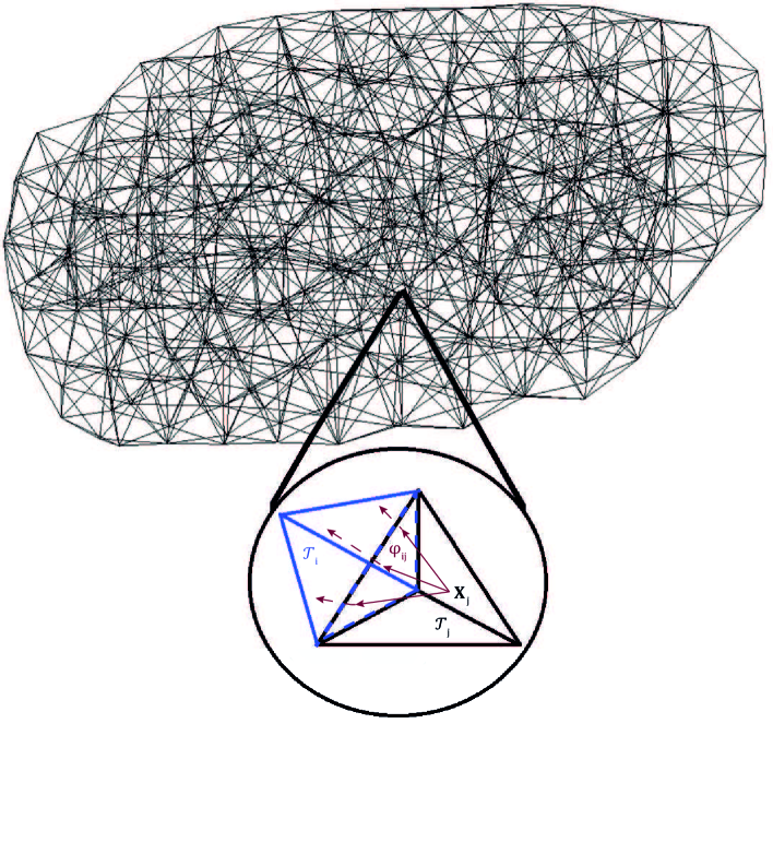
Figure 1: Discrete flow mapping on a mesh of a vehicle interior showing the boundary flow map $\boldsymbol{\varphi}_{ij}$ between the faces of a pair of adjacent tetrahedra. (Online version in colour.)

Consider the propagation of a density $f$ through a tetrahedral mesh $\mathcal{M}=\bigcup_{j=1}^{N}\mathcal{T}_{j}\subset\mathbb{R}^{3}$ consisting of $N$ tetrahedra $\mathcal{T}_{j}$, $j=1,...,N$, such as depicted in Fig. 1. Let us assume that the energy of the trajectory flow is governed by piecewise constant Hamiltonians of the form $H_{j}(\mathbf{r},\mathbf{p})=c_{j}|\mathbf{p}|=1$ in $\mathcal{T}_{j}$, where $c_{j}$ is the phase velocity for $\mathbf{r}\in\mathcal{T}_{j}$ and the momentum coordinate $\mathbf{p}$ lies on a sphere of radius $c_{j}^{-1}$. This Hamiltonian is associated with the Helmholtz equation with inhomogeneous wave velocity $c(\mathbf{r})$ (see [5]). We restrict our discussion to scalar propagation for simplicity; extensions to the vectorial wave equations arising in elasticity and electromagnetics are possible. In this case the wave propagation needs to be characterised by more than one Hamiltonian per tetrahedron.

Denote the phase space on the boundary of the tetrahedron $\mathcal{T}_{j}$ as $Q_{j}=\partial\mathcal{T}_{j}\times D_{1/c_{j}}$, where the notation $D_{R}$ refers to the open disk of radius $R$ and centre at the origin. Then the associated coordinates are given by $\mathbf{X}_{j}=[\mathbf{s}_{j},\mathbf{p}_{j}]\in Q_{j}$ with $\mathbf{s}_{j}\in\mathbb{R}^{2}$ parameterising $\partial\mathcal{T}_{j}$, the boundary of the $j$th tetrahedron, and $\mathbf{p}_{j}\in D_{1/c_{j}}$ parameterising the component of the inward momentum (or slowness) vector tangential to $\partial\mathcal{T}_{j}$. Next we define $\boldsymbol{\varphi}_{ij}:Q_{j}\rightarrow Q_{i}$ to be the boundary flow map, which takes a vector in $Q_{j}$ and maps it along the Hamiltonian flow given by $H_{j}$ to a vector in $Q_{i}$, see Fig. 1. Note that $\boldsymbol{\varphi}_{ij}$ is generally only defined on a subset of $\partial\mathcal{T}_{j}$ and only maps to a subset of $D_{1/c_{i}}$. The propagation of a density $f$ along the boundary flow map $\boldsymbol{\varphi}_{ij}$ is therefore given by the FP operator acting on this map as follows

$$\mathcal{L}f(\mathbf{X}_{i})=\sum_{j}\int_{Q_{j}}\delta(\mathbf{X}_{i}-\boldsymbol{\varphi}_{ij}(\mathbf{X}_{j}))f(\mathbf{X}_{j})\,\mathrm{d}\mathbf{X}_{j}.$$ (2)

The operator $\mathcal{L}$ describes propagation of $f$ along a trajectory with endpoint on the boundary of tetrahedron $\mathcal{T}_{i}$ and start point on the boundary of each neighbouring or coincident tetrahedron $\mathcal{T}_{j}$. In cases where a tetrahedral face is shared by the tetrahedra $\mathcal{T}_{i}$ and $\mathcal{T}_{j}$ with $i\neq j$, then a reflection/transmission law should be applied to specify the probability that the trajectory endpoint lies in each of $\partial\mathcal{T}_{i}$ and $\partial\mathcal{T}_{j}$. In order to include reflection/transmission along with other physics such as dissipation (or mode conversion for vectorial equations) we add a weighting function $w_{i,j}(\mathbf{X}_{j})$, see Eq. (4) below.

The stationary density $\rho(\mathbf{X}_{i})$ on $Q_{i}$, $i=1,...,N$, due to an initial boundary distribution $\rho_{0}$ on $Q_{j}$, $j=1,...,N$, is the density accumulated in the long time (many reflection) limit. That is

$$\rho(\mathbf{X}_{i})=\sum_{n=0}^{\infty}\mathcal{B}^{n}\rho_{0}(\mathbf{X}_{i}),$$ (3)

where $\mathcal{B}^{n}$ describes the transport of the initial density $\rho_{0}$ through $n$ reflections. Explicitly, $\mathcal{B}^{n}$ is the $n$th iterate of the operator $\mathcal{B}$ given by

$$\mathcal{B}f(\mathbf{X}_{i})=\sum_{j}\int_{Q_{j}}w_{i,j}(\mathbf{X}_{j})\delta(\mathbf{X}_{i}-\boldsymbol{\varphi}_{ij}(\mathbf{X}_{j}))f(\mathbf{X}_{j})\,\mathrm{d}\mathbf{X}_{j}.$$ (4)

In this work we consider only the case of deterministic propagation operators. Stochastic propagation may be described by replacing the $\delta$-distribution in (4) with a finite-width kernel (see for example Ref. [40]). If $w_{i,j}=1$, or more generally, if there are no dissipative terms and the initial phase space density is conserved, that is,

$$\sum_{i}\int_{Q_{i}}\left[\mathcal{B}^{n}\rho_{0}\right](\mathbf{X}_{i})\,\mathrm{d}\mathbf{X}_{i}\,=\sum_{i}\int_{Q_{i}}\rho_{0}(\mathbf{X}_{i})\,\mathrm{d}\mathbf{X}_{i}\,\quad\forall n,$$

then the operator $\mathcal{B}$ defined in (4) is of Frobenius-Perron type as in (2) with a maximum eigenvalue of 1. To obtain convergence of the sum in Eq. (3), a dissipative factor needs to be added; typically we apply an absorption factor of the form $\exp(-\mu_{j}L)$, where $L$ is the length of the trajectory and $\mu_{j}>0$ is the damping coefficient in tetrahedron $\mathcal{T}_{j}$. We also consider an example where the dissipative contribution is instead provided by an open boundary region.

In the case where the sum in Eq. (3) converges, then from the standard Neumann series result we have that the stationary density $\rho(\mathbf{X}_{i})$ may be computed by solving the following phase space boundary integral equation

$$(I-\mathcal{B})\rho(\mathbf{X}_{i})=\rho_{0}(\mathbf{X}_{i}).$$ (5)

Note that since the trajectory flow only maps to neighbouring tetrahedra, a matrix representation of $\mathcal{B}$ over the whole of $\bigcup_{i=1}^{N}Q_{i}$ is in general sparse. In the next section we design a discretisation strategy for efficiently computing such a matrix representation of $\mathcal{B}$ and hence numerically solving Eq. (5).

3 Discretisation

In this section we describe a finite basis approximation of the stationary density $\rho$ and the linear integral operator $\mathcal{B}$ defined in (4). We provide an algorithm for computing the entries of the resulting matrix representation $B$ of the operator $\mathcal{B}$. Furthermore, we describe a fast semi-analytic and semi-spectral integration strategy for computing the integrals arising in the definition of the entries in $B$.

3.1 Finite basis approximation

We consider a finite dimensional approximation of the stationary boundary density $\rho$ on $Q_{j}$ using a (product) basis expansion of the form

$$\rho(\mathbf{s}_{j},\mathbf{p}_{j})=\sum_{l=1}^{N_{j}}\sum_{n=0}^{N_{p}}\sum_{m=-n}^{n}\rho_{(j,l,n,m)}b_{l}(\mathbf{s}_{j})\tilde{Z}_{n}^{m}(\mathbf{p}_{j}),$$ (6)

where $N_{j}$ is the number of boundary elements on the tetrahedron $\mathcal{T}_{j}$. For simplicity, we assume that each triangular face forms a single element only and thus $N_{j}=4$ for all $j=1,\dots,N$. We note however that the precision of the spatial approximation may be improved by further sub-dividing the tetrahedral boundary faces. Also, $N_{p}$ is the order of the basis expansion in the direction coordinate $\mathbf{p}_{j}$. We apply orthonormal piecewise-constant basis functions $b_{l}$ in the space coordinate $\mathbf{s}_{j}$, with support only on $\bigtriangleup_{j,l}\subset\partial{\mathcal{T}_{j}}$, the $l^{\text{th}}$ boundary element on $\mathcal{T}_{j}$. Hence

$$b_{l}(\mathbf{s}_{j})=\frac{1}{\sqrt{|\bigtriangleup_{j,l}|}}$$

if $\mathbf{s}_{j}\in\bigtriangleup_{j,l}$ and is zero otherwise, where we use $|\bigtriangleup_{j,l}|$ to denote the area of $\bigtriangleup_{j,l}$. The functions $\tilde{Z}_{n}^{m}$ form an orthonormal basis in the direction coordinate $\mathbf{p}_{j}\in D_{1/c_{j}}$ and are given by

$$\tilde{Z}_{n}^{m}(\mathbf{p}_{j})=c_{j}Z_{n}^{m}(\tilde{\mathbf{p}}_{j}),$$ (7)

where $Z_{n}^{m}$ are the Zernike polynomials and $\tilde{\mathbf{p}}_{j}:=(\varrho_{j},\phi_{j})\in[0,1)\times[0,2\pi)$ is a re-scaling of $\mathbf{p}_{j}=(c_{j}^{-1}\varrho_{j},\phi_{j})$ to the unit disk.

In fact, there are many possible candidates for an orthogonal basis on a disc as outlined in Ref. [41]. The main advantages for the choice of Zernike polynomials here are their spectral convergence for interpolating analytic functions and their relative tractability in comparison with, for example, the Logan-Shepp ridge polynomials [41]. In addition, only half as many degrees of freedom are required to represent a complicated function on the disk compared with a Chebyshev- Fourier basis [41]. The latter property results from the fact that the inner sum in (6) only runs over the index values of the sum to $N_{p}$, and that $Z_{n}^{m}\equiv 0$ for $n-m$ odd.

The Zernike polynomials are defined as

$$Z_{n}^{m}(\tilde{\mathbf{p}}_{j}) =R_{n}^{m}(\varrho_{j})\cos(m\phi_{j}),\quad m\in\mathbb{Z}_{0}^{+},$$

$$Z_{n}^{m}(\tilde{\mathbf{p}}_{j}) =R_{n}^{|m|}(\varrho_{j})\sin(|m|\phi_{j}),\quad m\in\mathbb{Z}^{-},$$

where $n\in\mathbb{Z}_{0}^{+}$ and $R_{n}^{m}$ are polynomials of the radial coordinate only. Note that $R_{n}^{m}\equiv 0$ for $n-m$ odd, leading to the corresponding property for $Z_{n}^{m}$ described above. The relative tractability of the Zernike polynomials stems from the fact that their radial and angular dependence is separable into terms that can be easily calculated. The radial part is defined recursively via

$$R_{n}^{m}(\varrho)=\varrho\left(R_{n-1}^{|m-1|}(\varrho)+R_{n-1}^{m+1}(\varrho)\right)-R_{n-2}^{m}(\varrho),\quad R_{0}^{0}(\varrho)=1,\quad R_{1}^{1}(\varrho)=\varrho,$$

for any $\varrho\in[0,1]$ and the angular part is simply a trigonometric function. For completeness, note that the orthogonality property of Zernike polynomials (for $n-m$ even) is given by

$$\int_{0}^{2\pi}\int_{0}^{1}Z_{n}^{m}(\tilde{\mathbf{p}}_{j})Z_{n^{\prime}}^{m^{\prime}}(\tilde{\mathbf{p}}_{j})\,\varrho_{j}\mathrm{d}\varrho_{j}\mathrm{d}\phi_{j}=\frac{\epsilon_{m^{\prime}}\pi}{2n^{\prime}+2}\delta_{n,n^{\prime}}\delta_{m,m^{\prime}},$$

where $\epsilon_{m^{\prime}}=1$ for all $m^{\prime}\neq 0$ and $\epsilon_{0}=2$.

3.2 Discretisation of the integral operator $\mathcal{B}$

We apply a Galerkin projection of the operator $\mathcal{B}$ (4) onto the finite basis described above, which leads to a matrix representation $B$ with entries

$$B_{I,J}=\frac{2n^{\prime}+2}{\epsilon_{m^{\prime}}\pi}\int_{Q_{j}}w_{i,j}(\mathbf{X}_{j})\tilde{Z}_{n^{\prime}}^{m^{\prime}}(\boldsymbol{\varphi}_{p}(\mathbf{X}_{j}))b_{l^{\prime}}(\boldsymbol{\varphi}_{s}(\mathbf{X}_{j}))\tilde{Z}_{n}^{m}(\mathbf{p}_{j})b_{l}(\mathbf{s}_{j})\,\mathrm{d}\mathbf{X}_{j},$$ (8)

where the subscripts $I$ and $J$ denote multi-indices $I=(i,l^{\prime},n^{\prime},m^{\prime})$ and $J=(j,l,n,m)$, respectively. The boundary map $\boldsymbol{\varphi}_{i,j}=(\boldsymbol{\varphi}_{s},\boldsymbol{\varphi}_{p})$ is separated into spatial and directional components and the weight function $w_{i,j}$ contains absorption and reflection/transmission factors, as before. Once the entries of $B$ given in (8) have been computed, the approximation of the stationary boundary density $\rho$ is obtained by solving the linear system corresponding to the discrete form of equation (5) for the expansion coefficients $\rho_{(j,l,n,m)}$ in (6).

In order to write the entries of $B$ more explicitly in the form we compute them, we substitute (7) into (8) and perform a change of variables $\varrho_{j}=\sin(\theta_{j})$, where $\theta_{j}\in[0,\pi/2)$ is the angle of the trajectory with respect to the normal vector on $\bigtriangleup_{j,l}$. Furthermore, we write out fully the factors in the weight $w_{i,j}$ and separate the four integrals into two pairs to emphasise the relative simplicity of the spatial integrand as follows:

$$\begin{split}B_{I,J}=\frac{2n^{\prime}+2}{\epsilon_{m^{\prime}}\pi\sqrt{|\bigtriangleup_{j,l}||\bigtriangleup_{i,l^{\prime}}|}}\int_{0}^{2\pi}\int_{0}^{\pi/2}\lambda_{i,j}(\theta_{j},\phi_{j})Z_{n^{\prime}}^{m^{\prime}}(\tilde{\mathbf{p}}_{i}^{\prime})Z_{n}^{m}(\tilde{\mathbf{p}}_{j})\\ \left[\iint\limits_{\bigtriangledown_{j,l}}e^{-\mu_{j}L(\mathbf{s}_{j},\mathbf{s}^{\prime}_{i})}\,\mathrm{d}\mathbf{s}_{j}\right]\frac{\sin(2\theta_{j})}{2}\,\mathrm{d}\theta_{j}\,\mathrm{d}\phi_{j}.\end{split}$$ (9)

Here we have written $\boldsymbol{\varphi}_{i,j}(\mathbf{X}_{j})=[\boldsymbol{\varphi}_{s}(\mathbf{X}_{j}),\boldsymbol{\varphi}_{p}(\mathbf{X}_{j})]=[\mathbf{s}_{i}^{\prime},\mathbf{p}_{i}^{\prime}]$ for brevity and $L(\mathbf{s}_{j},\mathbf{s}^{\prime}_{i})$ is the Euclidean length of the trajectory connecting $\mathbf{s}_{j}$ and $\mathbf{s}_{i}^{\prime}$. Note that $\tilde{\mathbf{p}}_{i}^{\prime}$ is simply $\mathbf{p}_{i}^{\prime}$ after re-scaling to the unit disc. Furthermore, $\bigtriangledown_{j,l}\subseteq\bigtriangleup_{j,l}$ is the triangular subset of points in $\bigtriangleup_{j,l}$ that are mapped to $\bigtriangleup_{i,l^{\prime}}$ by $\boldsymbol{\varphi}_{ij}(\mathbf{X}_{j})$. Note that this subset depends on the direction of propagation $(\theta_{j},\phi_{j})$. The restriction of the spatial integration to $\bigtriangledown_{j,l}$ results from the basis function $b_{l^{\prime}}$ in (8) setting the integrand to zero for trajectories where $\mathbf{s}_{i}^{\prime}\notin\bigtriangleup_{i,{l^{\prime}}}$. In addition, we have separated the weight function into the product of the reflection/transmission probability $\lambda_{i,j}(\theta_{j},\phi_{j})$ and the absorption factor $\exp(-\mu_{j}L)$.

In the case of flat-faced polyhedra, the Euclidean length $L(\mathbf{s}_{j},\mathbf{s}^{\prime}_{i})$ is a linear function of $\mathbf{s}_{j}$ and hence the spatial integral over $\bigtriangledown_{j,l}$ can be computed analytically. We are then left with an integral over the unit disc to compute numerically. The strategy for performing the exact integration over the tetrahedral mesh element faces provides information about the regularity of the remaining integrand as a function of the direction coordinates. We describe this strategy in the next section and use it to motivate the design of a spectrally converging quadrature scheme for the outer integrals.

3.3 Computation of the matrix entries $B_{I,J}$

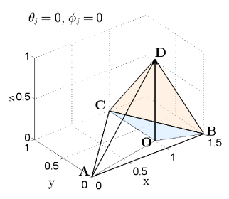
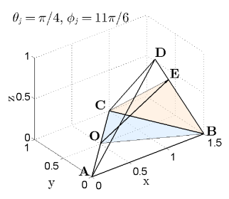
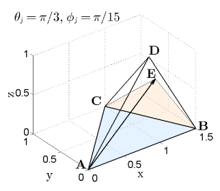
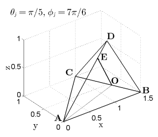
Figure 2: Tetrahedron with vertices $\mathbf{A}$, $\mathbf{B}$, $\mathbf{C}$ and $\mathbf{D}$. The shaded sub-regions show the admissible sets of start and end points for rays starting from face $ABC$ and arriving in face $CBD$. The set of admissible start points within triangle $ABC$ is equal to the spatial integration domain $\bigtriangledown_{j,l}$. Each of the four sub-plots shows these regions for a different fixed outgoing ray direction $(\theta_{j},\phi_{j})$. The trajectory of maximum length $L_{max}$ is indicated by the black arrow. Upper left: the set of admissible trajectory end-points is equal to the whole of $CBD$. Upper right: the sets of admissible start and end points are subsets of $ABC$ and $CBD$, respectively. Lower left: the set of admissible trajectory start points is equal to the whole of $ABC$. Lower right: the sets of admissible start and end points are both empty. (Online version in colour.)

In this section we describe the necessary steps for computing the four-dimensional integrals given in (9). For the purposes of illustration, consider a single tetrahedron with vertices $\mathbf{A}$, $\mathbf{B}$, $\mathbf{C}$ and $\mathbf{D}$ as shown in Fig. 2. The figure shows the admissible sets of start and end points for rays travelling in a specified fixed direction from face $ABC$ to face $CBD$. Each tetrahedral face has a prescribed local coordinate system with origin at one of the vertices (vertex $A$ in Fig. 2). The local $x$-axis is taken to be aligned with one of the edges (edge $AB$ in Fig. 2) and the local $z$-axis is taken parallel to the inward normal vector of the face. We rotate and translate each tetrahedron in the mesh, together with its neighbouring tetrahedra, such that the local face coordinates used for the spatial integration variables coincide with the global Cartesian coordinates as shown in Fig. 2.

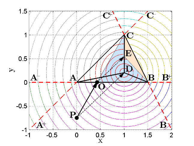
Figure 3: Tetrahedron with vertices $\mathbf{A}$, $\mathbf{B}$, $\mathbf{C}$ and $\mathbf{D}=({D}_{1},{D}_{2},{D}_{3})$ viewed from above. The dashed lines ${A^{-}B^{+}}$, ${B^{-}C^{+}}$ and ${C^{-}A^{+}}$ extend the three edges of triangle $ABC$ and demonstrate the subdivision of the $xy$-plane into seven sub-regions. For given direction $(\theta_{j},\phi_{j})$, the point $\mathbf{P}$ connects the $xy$-plane with vertex $\mathbf{D}$. If $\mathbf{P}$ lies outside the triangle $ABC$, then the point $\mathbf{O}$ is obtained by projecting $\mathbf{P}$ onto the boundary of $ABC$. Such points $\mathbf{P}$ span the $xy$-plane via circles of radius $D_{3}\tan(\theta_{j})$ and origin $(D_{1},D_{2})$. (Online version in colour.)

We first find the triangular region $\bigtriangledown_{j,l}\subseteq\bigtriangleup_{j,l}$ over which the spatial integration takes place, for a given direction $(\theta_{j},\phi_{j})$. Consider the upper left plot of Fig. 2, where the outgoing direction is parallel to the normal vector, that is, $\theta_{j}=0$. Here the point $\mathbf{O}$ forms the triangle $\bigtriangledown_{j,l}=OBC\subset ABC$ over which to perform the spatial integration. Outside this region ($OBC$) rays parallel to the normal direction $\mathbf{OD}$ will not approach face $BCD$, but instead approach one of the other two faces, $ABD$ or $CAD$. However, the point $\mathbf{O}$ may not be located inside the triangle $ABC$, but rather on the boundary of $ABC$ as shown in the other three plots of Fig. 2. The region $\bigtriangledown_{j,l}$ is therefore determined by finding the location of the point $\mathbf{O}$. In order to do this, first consider the point $\mathbf{P}$ in the local $xy$-plane such that the vector $\mathbf{PD}$ coincides with the direction vector specified by $(\theta_{j},\phi_{j})$, as illustrated in Fig. 3; this figure shows the tetrahedron from Fig. 2 viewed from above. We see that each direction value $(\theta_{j},\phi_{j})$ specifies a unique point $\mathbf{P}\in\mathbb{R}^{2}$. For example, when the angle $\theta_{j}$ is fixed but the angle $\phi_{j}$ varies from zero to $2\pi$, the points $\mathbf{P}$ lie on circles of radius $D_{3}\tan(\theta_{j})$ and have origin $(D_{1},D_{2})$, where $(D_{1},D_{2},D_{3})$ are the local coordinates of the point $\mathbf{D}$. We extend the three edges of $ABC$ as illustrated by the dashed lines in Fig. 3 and indicate the end-point limits of these infinitely extended dashed lines by $\mathbf{A}^{\pm}$, $\mathbf{B}^{\pm}$ and $\mathbf{C}^{\pm}$. The lines ${A^{-}B^{+}}$, ${B^{-}C^{+}}$ and ${C^{-}A^{+}}$ divide $\mathbb{R}^{2}$ into seven regions, and the region in which the point $\mathbf{P}$ lies prescribes one of seven possible locations for the point $\mathbf{O}$; the point $\mathbf{O}$ can be located either inside the triangle $ABC$, or on one of its three vertices, or along one of its three sides (not including the vertices).

In the simplest case, the point $\mathbf{P}$ already lies on or within the triangle $ABC$ and then $\mathbf{O}=\mathbf{P}$. On the other hand, if $\mathbf{P}$ lies in one of the three triangular areas, ${A^{-}AA^{+}}$, ${B^{-}BB^{+}}$ or ${C^{-}CC^{+}}$, then the point $\mathbf{O}$ is obtained by projecting $\mathbf{P}$ onto the vertex shared with triangle $ABC$. If the point $\mathbf{P}$ lies in one of the three quadrilateral areas, e.g. ${A^{+}ABB^{-}}$, then the point $\mathbf{O}$ is obtained by projecting the point $\mathbf{P}$ onto the edge shared with triangle $ABC$. This projection is taken along the line connecting the point $\mathbf{P}$ to the vertex of triangle $ABC$ not on the shared edge. In the illustrative example shown in Fig. 3, the point $\mathbf{O}$ is defined by the intersection of the lines $AB$ and $PC$.

In addition to finding the domain $\bigtriangledown_{j,l}$ for the spatial integrals in (9), we also need to find the maximal ray length between the two faces under consideration for a prescribed fixed direction $(\theta_{j},\phi_{j})$. In other words, we find

$$L_{max}=\max\left\{L(\mathbf{s}_{j},\mathbf{s}^{\prime}_{i})\right\},$$

where the distance function $L$ is expressed in the local coordinate system of $\bigtriangledown_{j,l}$. For example, consider the tetrahedron $ABCD$ in the upper-left plot of Fig. 2. Here, $L_{max}=D_{3}$ and we place the origin of the local coordinate system of triangle $OBC=\bigtriangledown_{j,l}$ at the vertex $\mathbf{B}$ such that the $x$-axis coincides with edge $BC$. More generally, when the point $\mathbf{O}$ lies inside the triangle $ABC$, then the ray of maximum length $L_{max}$ (indicated by a black arrow in Fig. 2) will intersect the vertex $\mathbf{D}$. If instead the point $\mathbf{O}$ lies on an edge of $ABC$ that is not on the destination face $CBD$, then the ray of maximum length will approach one of the edges of the destination face not on $ABC$ as depicted in the upper right plot of Fig. 2. When the point $\mathbf{O}$ coincides with the vertex $A$ of $ABC$ (not on the destination face $CBD$) as shown in the lower left plot of Fig. 2, then the longest ray will approach a point $\mathbf{E}$ inside the destination face and the spatial integration domain $\bigtriangledown_{j,l}=\bigtriangleup_{j,l}$. Finally, if the point $\mathbf{O}$ lies on an edge or vertex of the receiving face $CBD$, the region $\bigtriangledown_{j,l}=\emptyset$ and there is no need to compute $L_{max}$ since the corresponding contribution to the matrix entry $B_{I,J}$ is zero. Note therefore that the direction coordinate space is also divided into seven distinct sub-regions according to the seven possible locations for the point $\mathbf{O}$ on triangle $ABC$. For three of these sub-regions, the corresponding spatial integral will be zero as in the latter case described above.

Once we have obtained the integration domain $\bigtriangledown_{j,l}$ and the maximal ray length $L_{max}$, we can proceed with the analytical evaluation of the spatial integrals appearing in (9). These integrals have a relatively simple form since the distance function $L(\mathbf{s}_{j},\mathbf{s}^{\prime}_{i})$ is a linear function of the local coordinates of triangle $\bigtriangledown_{j,l}$. Considering again the tetrahedron $ABCD$ in the upper-left plot of Fig. 2 and taking $h$ to be the minimum distance from the point $\mathbf{O}$ to the edge $BC$, then in this case the spatial double-integral is given by

$$\iint\limits_{OBC}e^{-\mu_{j}L(\mathbf{s}_{j},\mathbf{s}^{\prime}_{i})}\,\mathrm{d}\mathbf{s}_{j}=\frac{h|\mathbf{BC}|}{(\mu_{j}L_{max})^{2}}\left(\mu_{j}L_{max}-1+e^{-\mu_{j}L_{max}}\right),\quad\mu_{j}>0.$$

In the case $\mu_{j}=0$, the integrand simplifies to unity and the integral is simply the area of the domain $\bigtriangledown_{j,l}$.

In order to complete the evaluation of the matrix entries $B_{I,J}$ in (9), we need to find the reflected/transmitted ray directions $\tilde{\mathbf{p}}_{i}^{\prime}=(\sin(\theta^{\prime}_{i}),\phi^{\prime}_{i})$ and compute the reflection/transmission probabilities $\lambda_{i,j}(\theta_{j},\phi_{j})$, before (numerically) integrating over $(\theta_{j},\phi_{j})$. We apply Snell’s Law to relate the reflection angle $\theta_{r}\in[0,\pi/2)$ to the transmission angle $\theta_{t}\in[0,\pi/2)$ via

$$\sin(\theta_{t})=\frac{c_{i}}{c_{j}}\sin(\theta_{r}).$$

The reflection angle $\theta_{r}$ corresponds to a specular reflection of the incoming ray. If $i=j$ then $\theta^{\prime}_{i}=\theta_{r}$, otherwise we have $\theta^{\prime}_{i}=\theta_{t}$. Once we have found $\theta^{\prime}_{i}$, then the azimuthal angle $\phi^{\prime}_{i}$ must be represented in the local coordinates of each face of the tetrahedral mesh using linear transformations of the incoming ray direction. We find that the reflection/transmission probability function is dependent only on reflection/transmission angles $\theta_{r}$ and $\theta_{t}$. For acoustic waves the transmission probability is given by

$$\lambda_{t}(\theta_{j},\phi_{j})=\frac{4z_{i}z_{j}\cos(\theta_{r})\cos(\theta_{t})}{(z_{i}\cos(\theta_{r})+z_{j}\cos(\theta_{t}))^{2}},$$

where the specific acoustic impedance $z_{j}=\rho^{f}_{j}c_{j}$ is the product of the fluid density $\rho_{j}^{f}$ and the propagation speed $c_{j}$ in tetrahedron $\mathcal{T}_{j}$. Then we have $\lambda_{i,j}=\lambda_{t}$ if $i\neq{j}$ and $\lambda_{i,i}=1-\lambda_{t}$.

Consider a quadrature rule for the integration over the direction coordinates $(\theta_{j},\phi_{j})$. For each pair $(\theta_{j},\phi_{j})$ specified by the quadrature rule, we carry out the following five steps:

1. Determine the triangular region $\bigtriangledown_{j,l}$.

2. Compute the maximal length of rays travelling from face $\bigtriangleup_{j,l}$ to face $\bigtriangleup_{i,{l^{\prime}}}$.

3. Compute the spatial (double) integral over the triangular area $\bigtriangledown_{j,l}$ analytically.

4. Find the reflection/transmission angles $(\theta^{\prime}_{i},\phi^{\prime}_{i})$ in the local face coordinates of $\mathcal{T}_{i}$.

5. Compute the Zernike polynomials $Z_{n}^{m}(\tilde{\mathbf{p}}_{j})$ and $Z_{n^{\prime}}^{m^{\prime}}(\tilde{\mathbf{p}}_{i}^{\prime})$, and the reflection/transmission function $\lambda_{i,j}(\theta_{j},\phi_{j})$.

The numerical integration strategy is further detailed in the next section.

3.4 Subdivision and parametrisation for the spectral quadrature scheme

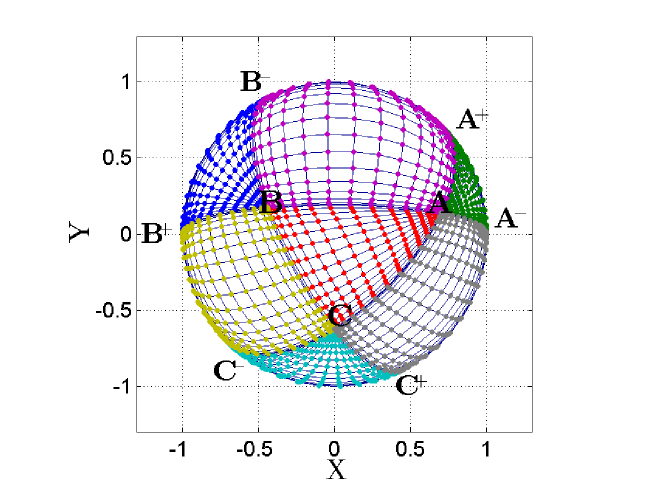
Figure 4: Seven subregions of the direction coordinate over the unit disc associated to the tetrahedron $ABCD$ presented in Figures 2 and 3. (Online version in colour.)

In this section we describe a subdivision and parametrisation of the direction space $(\theta_{j},\phi_{j})\in[0,\pi/2)\times[0,2\pi)$ in order to obtain a spectrally convergent quadrature scheme for the integrals with respect to $(\theta_{j},\phi_{j})$ appearing in Eq. (9). As described in the previous section, the seven regions in the local $xy$-plane indicated in Fig. 3 are associated with seven regions in the direction space on the unit disc as shown in Fig. 4, where the labelled points correspond to the points with the same labels shown in Fig. 3. Note that the lines ${A^{-}B^{+}}$, ${B^{-}C^{+}}$ and ${C^{-}A^{+}}$, which divide the seven regions, are great circles of the unit sphere depicted in Fig. 4. The spatial integral (as the function of direction) is smooth inside each of these subregions, but is only continuous along the lines dividing the subregions. This property serves as a good motivation for subdividing the integration in the direction coordinate into seven subregions as indicated in Fig. 4.

We now describe a suitable mapping and parameterisation for any of the seven subregions of the direction space illustrated in Fig. 4. The parametrisation of any triangular or rectangular region on the upper hemisphere can be achieved using a map of the form

$$\mathbf{f}(\xi,\eta)=\mathbf{a}+\mathbf{b}\xi+\mathbf{c}\eta+\mathbf{d}\xi\eta\in\mathbb{R}^{3},\quad(\xi,\eta)\in[-1,1]^{2},$$ (10)

with

$$\mathbf{a} =\frac{1}{4}(\mathbf{v}_{1}+\mathbf{v}_{2}+\mathbf{v}_{3}+\mathbf{v}_{4}),$$

$$\mathbf{b} =\frac{1}{4}(\mathbf{v}_{2}-\mathbf{v}_{1}+\mathbf{v}_{3}-\mathbf{v}_{4}),$$

$$\mathbf{c} =\frac{1}{4}(\mathbf{v}_{3}+\mathbf{v}_{4}-\mathbf{v}_{1}-\mathbf{v}_{2}),$$

$$\mathbf{d} =\frac{1}{4}(\mathbf{v}_{3}-\mathbf{v}_{4}+\mathbf{v}_{1}-\mathbf{v}_{2}),$$

and where $\mathbf{v}_{1}$, $\mathbf{v}_{2}$, $\mathbf{v}_{3}$ and $\mathbf{v}_{4}$ are four vertices on the upper-hemisphere. For a triangular region with vertices $\mathbf{v}_{1}$, $\mathbf{v}_{2}$ and $\mathbf{v}_{3}$, we simply set $\mathbf{v}_{4}=\mathbf{v}_{1}$. Then we map $\mathbf{f}(\xi,\eta)$ onto the upper-hemisphere using [42]

$$\mathbf{g}(\xi,\eta)=\frac{\mathbf{f}(\xi,\eta)}{|\mathbf{f}(\xi,\eta)|}.$$

Writing the entries of vectors $\mathbf{f}=(f_{1},f_{2},f_{3})^{T}$ and $\mathbf{g}=(g_{1},g_{2},g_{3})^{T}$, then we compute the direction $(\theta_{j},\phi_{j})$ as functions of $(\xi,\eta)$ via the standard relations for spherical coordinates:

$$\begin{split}\theta_{j}(\xi,\eta)&=\arccos(g_{3}(\xi,\eta)),\\ \phi_{j}(\xi,\eta)&=\mbox{mod}\left(\arctan\left(\frac{f_{2}(\xi,\eta)}{f_{1}(\xi,\eta)}\right),2\pi\right).\end{split}$$ (11)

In addition, the Jacobian of this transformation including the $\sin(2\theta_{j})/2$ factor appearing in (9) is given by

$${J}(\xi,\eta)=\frac{f_{3}}{|\mathbf{f}|^{4}}\>\mathrm{det}\left[\mathbf{f}\hskip 5.69054pt\frac{\partial\mathbf{f}}{\partial\xi}\hskip 5.69054pt\frac{\partial\mathbf{f}}{\partial\eta}\right].$$

Thus all sub-regions of direction space are reduced to two dimensional integrals over the square $[-1,1]^{2}$ and, in principle, any quadrature method can be applied. In our computations we consider a 2D adaptive Clenshaw-Curtis method. Clenshaw-Curtis quadrature converges spectrally if the integrand is sufficiently smooth. The splitting into seven sub-regions described above is however, not always sufficient to ensure this smoothness. If there is a change in propagation speed so that $c_{i}\neq c_{j}$ then the integration variable should be changed to the transmission direction in order to preserve the smoothness [43]. Another reason that a loss of regularity of the integrand may occur is that the spherical coordinate relation (11) leads to singularities in the $\phi_{j}$-dependent terms of the derivatives of the integrand in (9) when $\theta_{j}=0$. However, for sufficiently regular tetrahedral meshes, we observe spectral convergence of the Clenshaw-Curtis quadrature despite the singular behaviour near $\theta_{j}=0$. This is due to the fact that the Zernike polynomials $Z_{n}^{m}(\varrho_{j},\phi_{j})$ are equal to zero at $\theta_{j}=0$ for any $m\neq 0$ (recall $\varrho_{j}=\sin(\theta_{j})$). Furthermore, $Z_{n}^{0}(0,\phi_{j})=(-1)^{n/2}$ and is thus independent of $\phi_{j}$. For irregular tetrahedral meshes containing long slender tetrahedra, the singularity may still cause numerical issues. In this case, a change of variables using functions that are flat at $\theta_{j}=0$ (that is, their derivatives vanish at $\theta_{j}=0$) can be introduced to remove the singularity in higher derivatives of integrand [44].

4 Numerical results

In this section we present results for two numerical examples. Firstly, we consider one-dimensional trajectory propagation in a cuboid, since here we can compare our result with both an exact geometric solution and an averaged wave solution. Secondly, we simulate the high frequency response of a vehicle cavity to a point source excitation. Through both numerical results we demonstrate the efficiency of DFM on tetrahedral meshes and the convergent behaviour of the solution as the Zernike polynomial direction basis order is increased.

4.1 Verification for a cuboid cavity

As a first example we consider a density distribution inside a cuboid $(x,y,z)\in(0,\ell)\times(-0.5,0.5)\times(-0.5,0.5)$. We prescribe a constant ray density along the boundary surface of the cuboid at $x=0$ with a fixed inward direction taken along the normal direction $(1,0,0)$. At all other boundaries of the cuboid we prescribe a homogeneous Neumann (or sound hard) boundary condition. This leads to a one-dimensional solution along the $x$-axis, which is independent of $y$ and $z$. Due to the geometric simplicity, this example possesses both an exact geometrical optics solution and an exact wave equation solution that we will compare against the numerical DFM solutions for different orders of Zernike polynomial basis approximation.

The exact solution $u$ for the associated wave problem is given by solving a two-point Neumann boundary value problem for the Helmholtz equation with complex wavenumber $k=\omega/c+i\mu/2$. Here $\omega$ is the angular frequency, $c$ is the wave speed and $\mu=\eta\omega/(2c)$ is a frequency-dependent dissipation rate with (hysteretic) loss factor $\eta$. It is reasonably straightforward to show that the solution with a unit Neumann condition at $x=0$ and a homogeneous (Neumann) condition at $x=\ell$ is given by a sum of left and right travelling plane waves as

$$u(x;\omega)=\frac{1}{2k\sin(k\ell)}(e^{ik(x-\ell)}+e^{ik(\ell-x)}).$$ (12)

Assuming that $u$ defines a velocity potential in a fluid of density $\rho^{f}$, then the acoustic energy density is given by $\rho^{f}\omega^{2}|u|^{2}/c^{2}$ and the averaged acoustic energy density over a frequency band $[\omega-\Delta\omega/2,\omega+\Delta\omega/2]$ can be calculated via

$$\rho_{\omega}(x)=\frac{\rho^{f}}{c^{2}\Delta\omega\,}\int_{\omega-\Delta\omega/2}^{\omega+\Delta\omega/2}q^{2}|u(x;q)|^{2}\,\mathrm{d}q.$$ (13)

The corresponding ray tracing model arises by transporting a source density $\tilde{\rho}_{0}$ from $x=0$ towards $x=\ell$, where it is reflected back towards $x=0$. After being transported though $n$ reflections at both $x=\ell$ and $x=0$ (after returning), the ray density travelling from left to right is given by

$$\rho_{+}^{n}(x)=e^{-\mu(2\ell n+x)}\tilde{\rho}_{0},\quad n=0,1,2\dots$$

Likewise, the ray density travelling from right to left at the point $x$ after $n$ reflections at $x=\ell$ is given by

$$\rho_{-}^{n}(x)=e^{-\mu(2\ell n-x)}\tilde{\rho}_{0},\quad n=1,2\dots$$

The final stationary density $\rho^{*}(x)$ is accumulated from the contributions from both directions after each reflection and leads to a geometric series solution of the form

$$\rho^{*}(x)=\sum_{n=0}^{\infty}\rho_{+}^{n}(x)+\sum_{n=1}^{\infty}\rho_{-}^{n}(x)=\frac{e^{-\mu x}+e^{-\mu(2\ell-x)}}{1-e^{-2\mu\ell}}\tilde{\rho}_{0}.$$ (14)

A source density $\tilde{\rho}_{0}$ corresponding to the boundary condition for the averaged wave solution (13) can be found by setting $\rho^{*}(0)=\rho_{\omega}(0)$. Applying this condition and combining (13) and (14) at $x=0$ leads to

$$\tilde{\rho}_{0}=\tanh(\mu\ell)\rho_{\omega}(0).$$

Note that for large $\omega$ and hence large $\mu$, $\tanh(\mu\ell)\sim 1$ and we have simply that $\tilde{\rho}_{0}\sim\rho_{\omega}(0)$. Physically, this corresponds to the solution being dominated by the initial plane wave travelling from left to right, since the high damping leads to a negligible contribution from the returning reflected waves. In this high frequency limit, one can also derive a frequency independent source density as

$$\rho_{\omega}(0)\sim\frac{\rho^{f}}{1+\eta^{2}/16}.$$

In the 3D DFM simulations we prescribe a constant initial density value $\tilde{\rho}_{0}$ across the face of the cuboid at $x=0$ with fixed direction parallel to the surface normal, that is we lift $\tilde{\rho}_{0}$ to phase space via

$$\rho_{0}=\tilde{\rho}_{0}\frac{\delta(\varrho_{j})}{2\pi\varrho_{j}}.$$ (15)

Recall $\varrho_{j}=\sin(\theta_{j})$ and note that the delta distribution has been normalised for polar coordinates so that

$$\int_{0}^{2\pi}\int_{0}^{1}\frac{\delta(\varrho_{j})}{2\pi\varrho_{j}}\varrho_{j}\,\mathrm{d}\varrho_{j}\,\mathrm{d}\phi_{j}=1.$$

The initial density (15) is then projected onto the finite basis approximation (6) in order to perform the numerical simulations.

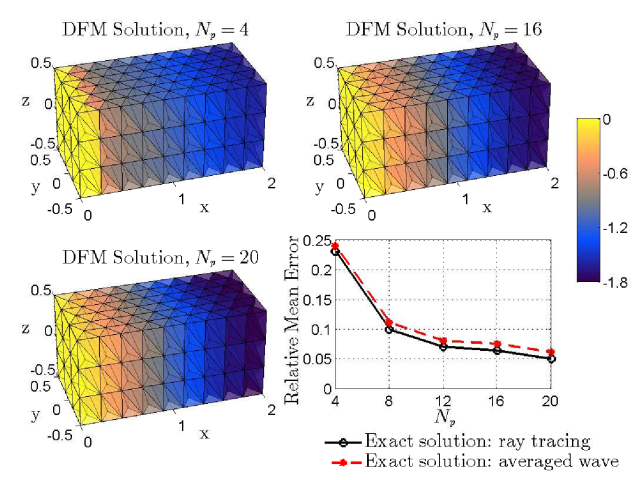
Figure 5: The interior density $\rho_{\mathcal{T}}$ (see Eq. (16)) in a cuboid mesh with parameter values $N=972$, $\omega=200\pi$, $\eta=0.004$, $\rho_{j}^{f}=1$ and $c_{j}=1$ for all $j=1,\ldots,N$. The first three plots show the DFM simulation results for $\log(\rho_{\mathcal{T}}(\mathbf{r}))$ with $\mathbf{r}$ chosen as the centroid of each tetrahedron and with Zernike polynomial direction basis order $N_{p}=4$ (upper left), $N_{p}=16$ (upper right) and $N_{p}=20$ (lower left). The lower right plot shows the relative mean error of DFM simulations for different approximation orders where the exact solution is given by either the exact ray density solution (14) or the averaged exact wave solution (13). (Online version in colour.)

The numerical results for a cuboid with $\ell=2$ are shown in Fig. 5. We employ a tetrahedral mesh with $N=972$ elements and choose the fluid density and the propagation speed to be $\rho^{f}_{j}=c_{j}=1$ for all $j=1,\ldots,N$. We also take $\omega=200\pi$ and apply a loss factor of $\eta=0.004$. The numerical integrals are evaluated using a spectrally convergent Clenshaw-Curtis rule on appropriately defined sub-regions. Figure 5 shows the interior stationary density $\rho_{\mathcal{T}}$ plotted on a logarithmic scale. This interior density may be computed at $\mathbf{r}\in\mathcal{T}_{j}$ by projecting the stationary boundary density $\rho$ onto the interior position space via

$$\rho_{\mathcal{T}}(\mathbf{r})=\frac{1}{c_{j}^{3}}\sum_{l=1}^{4}\int_{\bigtriangleup_{j,l}}\rho(\mathbf{s}_{j},\mathbf{p}_{j})\frac{\cos(\vartheta(\mathbf{s}_{j},\mathbf{r}))}{|\mathbf{r}-\mathbf{r}_{s_{j}}|^{2}}e^{-\mu_{j}|\mathbf{r}-\mathbf{r}_{s_{j}}|}\,\mathrm{d}\mathbf{s}_{j}.$$ (16)

Here $\mathbf{r}_{s_{j}}\in\mathbb{R}^{3}$ are the Cartesian coordinates of the point $\mathbf{s}_{j}\in\partial\mathcal{T}_{j}$ and $\vartheta(\mathbf{s}_{j},\mathbf{r})\in[0,\pi/2)$ is the angle between the normal vector to $\bigtriangleup_{j,l}$ (pointing into $\mathcal{T}_{j}$) and the direction vector $\mathbf{r}-\mathbf{r}_{s_{j}}$.

The first three plots of Fig. 5 show the interior density results computed at the centroid of each tetrahedron. The DFM result with $N_{p}=4$ shown in the upper-left plot clearly differs from the two higher order computations shown in the upper-right and lower-left plots. The discrepancy is most clear towards the right of the cavity where the energy density has not decayed to the level shown in the other plots. The plots with $N_{p}=16$ and $N_{p}=20$ are very similar suggesting that the solution is reasonably well converged on this particular mesh. The lower-right plot shows the relative mean error, that is, the mean absolute error divided by the mean of the exact solution taken over all tetrahedra in the mesh. The errors are plotted for various approximation orders from $N_{p}=4$ to $N_{p}=20$ and suggest convergence towards a solution with around $5\%$ error compared to the exact ray density solution (14) and around $6\%$ error with reference to the averaged exact wave solution (13). The exact solutions themselves are not plotted in Fig. 5, since they have a very similar appearance to the higher order DFM results. The averaged exact wave solution was calculated using a frequency band of $\Delta\omega=20\pi$ and the larger error in this case can be attributed to the geometrical optics approximation of the wave problem. The fact that the errors in both cases are fairly similar suggests that a ray-based model is appropriate for this problem.

The results presented could be improved by using a finer tetrahedral mesh and increasing the Zernike polynomial approximation order until the error appears to be saturating as above. Alternatively, one could consider subdividing the tetrahedral faces and applying the piecewise constant spatial basis over smaller boundary elements of the tetrahedral boundary as discussed in Sect. 3.1, or employing higher order basis approximations in space as discussed for two-dimensional problems in Ref. [43]. We also note that a relatively low damping level with loss factor $\eta=0.004$ has been applied and that for larger damping values the solution would decay more quickly from left to right. In this case a finer spatial approximation using one of the methods described above would be required to achieve the accuracy level shown in Fig. 5. Using an error tolerance of $10^{-4}$ for the numerically evaluated integrals, the computational times for the results presented above are around 90s for the $N_{p}=4$ result, 100 minutes for $N_{p}=16$ and 300 minutes for $N_{p}=20$.

The cuboid example considered in this section is highly directional with propagation only along the $x$–direction and thus poses a great challenge for modelling with DFM, which approximates the whole direction space using a smooth basis. In fact, DFM is particularly suited to modelling complex structures with many reflections where the dependence of the solution on the direction of propagation will be far smoother. Such an example will be considered in the next section. Despite its limitations for such highly directive problems, we note that DFM was able to reproduce the qualitative solution behaviour to a reasonable level of accuracy.

4.2 Application to a tetrahedral mesh of a vehicle cavity

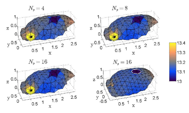
Figure 6: The DFM results for the interior density $\rho_{\mathcal{T}}$ in a vehicle cavity mesh with parameter values $N=1300$, $\omega=200\pi$, $\rho^{f}_{j}=1$, $c_{j}=1$ and $\mu_{j}=0$ for all $j=1,\ldots,N$. The plotted quantity is $\log(\rho_{\mathcal{T}}(\mathbf{r}))$ with $\mathbf{r}$ chosen as the centroid of each tetrahedron. The boundary of an opening in the upper part of the cavity is indicated in white on the lower right plot. The other three plots all show the cavity sliced approximately through the centre; only tetrahedra with centroids in the half-space $y>0$ are plotted. The source point at $r_{0}=(0.56467,0.024773,0.28073)$ is therefore visible in these three plots and is indicated by a black spot. The results are shown with Zernike polynomial direction basis order $N_{p}=4$ (upper left), $N_{p}=8$ (upper right) and $N_{p}=16$ (both lower plots). (Online version in colour.)

In this section we present the results of DFM simulations in a vehicle cavity discretised by $N=1300$ tetrahedral mesh elements as shown in Fig. 6. The cavity is excited with an interior point source and is assumed to have a specularly reflecting (outer) boundary where energy is conserved, except for a small open region in the roof through which energy is lost. We place the source point $\mathbf{r}_{0}$ at one of the mesh vertices $\mathbf{r}_{0}=(0.56467,0.024773,0.28073)$, which is located towards the front of the vehicle cavity. The point source velocity potential gives rise to an acoustic energy density on the boundary of any neighboring tetrahedra $\mathcal{T}_{j}$ of the form

$$\rho_{0}(\mathbf{s}_{j},\mathbf{p}_{j};\mathbf{r}_{0})=\frac{\rho^{f}_{j}\omega^{2}\cos(\vartheta(\mathbf{s}_{j},\mathbf{r}_{0}))\delta(\mathbf{p}_{j}-\mathbf{p}_{0}(\mathbf{s}_{j},\mathbf{r}_{0}))}{16\pi^{2}c_{j}|\mathbf{r}_{0}-\mathbf{r}_{s_{j}}|^{2}}e^{-\mu_{j}|\mathbf{r}_{0}-\mathbf{r}_{s_{j}}|},$$ (17)

where $\mathbf{r}_{s_{j}}\in\mathbb{R}^{3}$ are the Cartesian coordinates of $\mathbf{s}_{j}\in\partial\mathcal{T}_{j}$ as before and $\mathbf{p}_{0}(\mathbf{s}_{j},\mathbf{r}_{0})\in D_{1/c_{j}}$ is the tangential part of the momentum vector with direction $\mathbf{r}_{0}-\mathbf{r}_{s_{j}}$. In this example we set $\mu_{j}=0$ for all $j=1,\ldots,N$; note that the dissipation required for the sum in Eq. (3) to converge is provided via the losses through the open boundary region instead. The boundary of the opening is illustrated in white in the lower right plot of Fig. 6.

In order to perform the DFM computation, we project the source boundary density (17) onto the finite basis approximation (6). We fix $\rho^{f}_{j}=c_{j}=1$, and compute all numerical integrals to single precision using spectrally convergent Clenshaw-Curtis quadrature. We consider Zernike polynomial basis orders $N_{p}=4,8$ and $16$. A cross-section of the cavity with the source point indicated by a black spot is shown in the first three plots of Fig. 6, while the final plot (lower-right) illustrates the whole cavity. In the first three plots the cavity is sliced approximately through the centre in the $y$-direction, and only tetrahedra whose centroids are located in the half-space $y>0$ are plotted. The interior density is computed at the centroid of each tetrahedron and plotted on a logarithmic scale as before. The computational results for approximation orders $N_{p}=8$ and $N_{p}=16$ are very similar and illustrate the convergence of the DFM result on this particular mesh. These higher order computations indicate a stronger shadowing effect underneath the open boundary region, compared with the result for $N_{p}=4$. Increasing the order of the approximation in direction space therefore better captures the loss of energy through the non-reflecting region, causing less energy to propagate into the cavity immediately underneath to the opening.

We note that the 3D DFM simulations presented here are vastly more computationally efficient than the 3D DEA simulations presented in [35]. The largest computation presented in this section ($N_{p}=16$) took approximately $10$ hours to run using a MATLAB implementation of the code. A similar computation on a simpler cavity using only a second order basis approximation in momentum took several weeks using the 3D DEA method reported in [35]. It should be noted that DFM is also easily parallelisable using a simple parameter sweep over the tetrahedra $j=1,\ldots,N$ and hence the computational time could be improved further by performing parallelised computations within a high performance programming language. We also note that although the problems modelled in this work have used conforming tetrahedral meshes, an extension to non-conforming meshes would simply be a case of ensuring that the trajectory flows are associated to the appropriate destination tetrahedra. Furthermore, the feasibility of the exact spatial integration method relies only on linearity and not on the tetrahedral geometry itself; extensions to general convex polyhedra would be possible but more complicated to implement.

5 Conclusions

We have extended the DFM approach described in [36] to model wave energy densities in three-dimensional domains. In DFM, the densities to be computed are transported along ray trajectories through tetrahedral mesh elements using a finite dimensional approximation of a ray transfer operator. The relative geometric simplicity of the tetrahedral mesh elements has been exploited to efficiently compute the entries in the matrix representation of the discretised ray transfer operator. In particular, each matrix entry requires the evaluation of a four-dimensional integral; two integrals have been evaluated analytically, and the other two have been computed using spectrally convergent quadrature methods. Numerical results have been presented to verify the methodology, and to demonstrate its convergence and efficiency in practice for a full-scale vehicle cavity mesh provided by an industrial collaborator.

References

- [1] A. Sestieri and A. Carcaterra, “Vibroacoustic: The challenges of a mission impossible?,” Mech. Syst. Signal Pr., vol. 34, no. 1–2, pp. 1–18, 2013.
- [2] G. Tanner, “The future of high-frequency vibro-acoustic simulation methods in engineering applications,” in Proceedings of NOVEM 2015, (Dubrovnik, Croatia), April 2015.
- [3] G. Gradoni, S. C. Creagh, G. Tanner, C. Smartt, and D. W. P. Thomas, “A phase-space approach for propagating field-field correlation functions,” New J. Phys., vol. 17, no. 9, p. 093027, 2015.
- [4] M. I. Montrose, EMC and the Printed Circuit Board: Design, Theory, and Layout Made Simple. Chichester: John Wiley and Sons, 1998.
- [5] O. Runborg, “Mathematical models and numerical methods for high frequency waves,” Comm. Comp. Phys., vol. 2, no. 5, pp. 827–880, 2007.
- [6] D. J. Chappell and G. Tanner, “Solving the stationary Liouville equation via a boundary element method,” J. Comp. Phys., vol. 234, pp. 487–498, 2013.
- [7] V. Červený, Seismic Ray Theory. Cambridge: Cambridge University Press, 2001.
- [8] S. Osher and R. P. Fedkiw, “Level set methods: An overview and some recent results,” J. Comp. Phys., vol. 169, no. 2, pp. 463–502, 2001.
- [9] B. Engquist and O. Runborg, “Computational high frequency wave propagation,” Acta Numerica, vol. 12, pp. 181–266, 5 2003.
- [10] L. Ying and E. J. Candés, “The phase flow method,” J. Comp. Phys., vol. 220, no. 1, pp. 184–215, 2006.
- [11] G. Tanner, “Dynamical energy analysis – determining wave energy distributions in vibro-acoustical structures in the high-frequency regime,” J. Sound Vib., vol. 320, no. 4–5, pp. 1023–1038, 2009.
- [12] A. Celani, M. Cencini, A. Mazzino, and M. Vergassola, “Active and passive fields face to face,” New J. Phys., vol. 6, no. 1, p. 72, 2004.
- [13] M. Sommer and S. Reich, “Phase space volume conservation under space and time discretization schemes for the shallow-water equations,” Mon. Weather Rev., vol. 138, pp. 4229–4236, 2010.
- [14] P. Cvitanović, R. Artuso, R. Mainieri, G. Tanner, and G. Vattay, Chaos: Classical and Quantum. Copenhagen: Niels Bohr Institute, 2012. http://ChaosBook.org.
- [15] A. L. Bot, “Energy transfer for high frequencies in built-up structures,” J. Sound Vib., vol. 250, no. 2, pp. 247–275, 2002.
- [16] S. Siltanen, T. Lokki, S. Kiminki, and L. Savioja, “The room acoustic rendering equation,” J. Acoust. Soc. Amer., vol. 122, pp. 1624–1635, 2007.
- [17] J. Ding and A. Zhou, “Finite approximations of Frobenius-Perron operators. a solution of Ulam’s conjecture to multi-dimensional transformations,” Physica D, vol. 92, no. 1-2, pp. 61–68, 1996.
- [18] C. Bose and R. Murray, “The exact rate of approximation in Ulam’s method,” Discrete Continuous Dyn. Syst., vol. 7, no. 1, pp. 219–235, 2001.
- [19] M. Blank, G. Keller, and C. Liverani, “Ruelle-Perron-Frobenius spectrum for anosov maps,” Nonlinearity, vol. 15, no. 6, p. 1905, 2002.
- [20] O. Junge and P. Koltai, “Discretization of the Frobenius-Perron operator using a sparse Haar tensor basis: The sparse Ulam method,” SIAM J. Numer. Anal., vol. 47, no. 5, pp. 3464–3485, 2009.
- [21] G. Froyland, O. Junge, and P. Koltai, “Estimating long term behavior of flows without trajectory integration: the infinitesimal generator approach,” SIAM J. Numer. Anal., vol. 51, no. 1, pp. 223–247, 2013.
- [22] D. Lippolis and P. Cvitanović, “How well can one resolve the state space of a chaotic map?,” Phys. Rev. Lett., vol. 104, p. 014101, Jan 2010.
- [23] F. Noé, C. Schütte, E. Vanden-Eijnden, L. Reich, and T. R. Weikl, “Constructing the equilibrium ensemble of folding pathways from short off-equilibrium simulations,” Proc. Nat. Acad. Sci. USA, vol. 106, pp. 19011–19016, 2009.
- [24] S. Chandrasekhar, Radiative transfer. New York: Dover, 1960.
- [25] S. T. Thynell, “Discrete-ordinates method in radiative heat transfer,” Int. J. Eng. Sci., vol. 36, no. 12–14, pp. 1651–1675, 1998.
- [26] J. T. Kayija, “The rendering equation,” in Proceedings of SIGGRAPH 1986, vol. 20, pp. 143–150, 1986.
- [27] A. L. Bot, “A vibroacoustic model for high frequency analysis,” J. Sound Vib., vol. 211, no. 4, pp. 537–554, 1998.
- [28] R. Lyon, “Statistical analysis of power injection and response in structures and rooms,” J. Acoust. Soc. Amer., vol. 45, pp. 545–565, 1969.
- [29] R. Lyon and R. DeJong, Theory and Application of Statistical Energy Analysis. Boston: Butterworth-Heinemann, 1995.
- [30] T. Lafont, N. Totaro, and A. Le Bot, “Review of statistical energy analysis hypotheses in vibroacoustics,” Proc. Roy. Soc. A, vol. 470, no. 2162, 2013.
- [31] G. Gradoni, J.-H. Yeh, B. Xiao, T. M. Antonsen, S. M. Anlage, and E. Ott, “Predicting the statistics of wave transport through chaotic cavities by the random coupling model: A review and recent progress,” Wave Motion, vol. 51, no. 4, pp. 606–621, 2014. Innovations in Wave Modelling.
- [32] R. S. Langley, “A wave intensity technique for the analysis of high frequency vibrations,” J. Sound Vib., vol. 159, no. 3, pp. 483–502, 1992.
- [33] R. S. Langley and A. N. Bercin, “Wave intensity analysis of high frequency vibrations,” Phil. Trans. Roy. Soc. A, vol. 346, no. 1681, pp. 489–499, 1994.
- [34] A. L. Bot, “Energy exchange in uncorrelated ray fields of vibroacoustics,” J. Acoust. Soc. Amer., vol. 120, no. 3, pp. 1194–1208, 2006.
- [35] D. J. Chappell, G. Tanner, and S. Giani, “Boundary element dynamical energy analysis: A versatile method for solving two or three dimensional wave problems in the high frequency limit,” J. Comp. Phys., vol. 231, no. 18, pp. 6181–6191, 2012.
- [36] D. J. Chappell, G. Tanner, D. Löchel, and N. Søndergaard, “Discrete flow mapping: transport of phase space densities on triangulated surfaces,” Proc. Roy. Soc. A, vol. 469, no. 2155, 2013.
- [37] D. J. Chappell, D. Löchel, N. Søndergaard, and G. Tanner, “Dynamical energy analysis on mesh grids: A new tool for describing the vibro-acoustic response of complex mechanical structures,” Wave Motion, vol. 51, no. 4, pp. 589–597, 2014. Innovations in Wave Modelling.
- [38] G. Tanner and D. Chappell, “Discrete flow mapping - extending DEA towards an efficient mesh based simulation tool for high-frequency vibro-acoustics,” in Proceedings of ISMA2014 - USD2014, (Leuven, Belgium), pp. 2373–2382, September 2014.
- [39] J. Bajars, D. Chappell, N. Søndergaard, and G. Tanner, “Computing high-frequency wave energy distributions in two and three dimensions using discrete flow mapping,” in Proceedings of the 22nd International Congress on Sound and Vibration (ICSV22), (Florence, Italy), July 2015.
- [40] D. Chappell and G. Tanner, “A boundary integral formalism for stochastic ray tracing in billiards,” Chaos, vol. 24, no. 4, p. 043137, 2014.
- [41] J. P. Boyd and F. Yu, “Comparing seven spectral methods for interpolation and for solving the Poisson equation in a disk: Zernike polynomials, Logan-Shepp ridge polynomials, Chebyshev-Fourier series, cylindrical Robert functions, Bessel-Fourier expansions, square-to-disk conformal mapping and radial basis functions,” J. Comp. Phys., vol. 230, no. 4, pp. 1408–1438, 2011.
- [42] N. Boal, V. Dominguez, and F.-J. Sayas, “Asymptotic properties of some triangulations of the sphere,” J. Comp. Appl. Math., vol. 211, no. 1, pp. 11–22, 2008.
- [43] J. Bajars, D. Chappell, T. Hartmann, and G. Tanner, “High order approximation of phase-space densities on triangulated domains using discrete flow mapping,” Submitted, 2016.
- [44] P. Davis and P. Rabinowitz, Methods of Numerical Integration. Mineola, NY: Dover, 2nd ed., 1984.