Resilience of $\mathcal{PT}$ symmetry against stochasticity in a gain-loss balanced oscillator

Abstract

We investigate the effects of dichotomous noise added to a classical harmonic oscillator in the form of stochastic time-dependent gain and loss states, whose durations are sampled from two distinct exponential waiting time distributions. Despite the stochasticity, stability criteria can be formulated when averaging over many realizations in the asymptotic time limit and serve to determine the boundary line in parameter space that separates regions of growing amplitudes from those of decaying ones. Furthermore, the concept of $\mathcal{PT}$ symmetry remains applicable for such a stochastic oscillator and we use it to distinguish between an underdamped symmetric phase and an overdamped asymmetric phase. In the former case, the limit of stability is marked by the same average duration for the gain and loss states, whilst in the the latter case, a higher duration of the loss state is necessary to keep the system stable. The overdamped phase has an ordered structure imposing a position-velocity ratio locking and is viewed as a phase transition from the underdamped phase, which instead displays a broad and more disordered, but nevertheless, $\mathcal{PT}$ symmetric structure. We also address the short time limit and the dynamics of the moments of the position and the velocity with the aim of revealing the extremely rich dynamics offered by this apparently quite simple mechanical system. The notions established so far may be extended and applied in the stabilization of light propagation in metamaterials and optical fibres with randomly distributed regions of asymmetric active and passive media.

• August 2016

Keywords: Stochastic oscillators, Dichotomous noise, PT-symmetry, Phase transition.

1 Introduction

Given that physical systems are in general not conservative but rather tend to dissipate energy, some external forces are always necessary in order to reactivate their dynamics. There exist many systems, such as the simple pendulum, a motor engine or electric circuit that undergo transitions between states in which energy is gained and dissipated. If the gain is tunable enough in order to compensate the loss, then the resulting device simulates perfectly a conservative system and thus preserves the time reversal symmetry ${\mathcal{T}}$ but for many reasons, mostly technical (regulation or automatism), the compensation is not always perfect so that the loss and gain have to be treated separately.

However, even an imperfect control of the energy balance can result in extraordinary new properties. Indeed, let us consider a system that switches between two possible states, one in which energy is gained and the other where energy is lost. It is clear that such a system breaks the time reversal invariance ${\mathcal{T}}$ and looses its nice property of energy conservation. What is more obvious is that it is not invariant under the operation ${\mathcal{P}}$ which consists in a swap between the loss and gain states. Yet, in order to preserve some symmetry, one idea is to combine the two operations and impose on the non-conservative system a weaker requirement of invariance under the $\mathcal{PT}$ transformation.

Works involving $\mathcal{PT}$ symmetry have been initiated in the context of quantum mechanics using non Hermitian Hamiltonians [1] in which ${\mathcal{P}}$ refers to the parity operator, which reverses the position. The investigation of a generic class of $\mathcal{PT}$ symmetric Hamiltonians has shown that their energy spectrum remains real below a critical point but becomes imaginary beyond it, manifesting a transition to new ’exotic’ quantum states. Subsequent works [1, 2, 3, 4] have led to a reformulation of the use of these concepts in the framework of a non-Hermitian model involving only two quantum states for which the parity operator corresponds to the swap operation between the two states.

Since these seminal works [1, 2, 5, 6, 7], this new field has emerged in other contexts such as classical optics and electrical circuits in order to better understand the interplay between active and passive transmission, but also in tight binding systems [8, 9, 10]. In optical fibers, the simultaneous use of active and passive components displays very interesting properties such as transient wave amplification in an array of coupled waveguides with an arbitrary space distribution of gain and loss [11]. Furthermore, there are experiments which demonstrated that $\mathcal{PT}$ symmetric materials can exhibit power oscillations, non-reciprocal light propagation and tailored energy flow [6, 7, 12]. In addition, the existence of giant amplifications is predicted, meaning that a passive medium may be helpful to enhance the gain effect of an active medium [13]. Similar problems were studied in another experiment with a pair of coupled oscillators in the form of an $LRC$ circuit [12]. Instead of considering a single oscillator that switches between gain and loss states, the authors of [12] examined an electronic dimer made of two coupled oscillators, one with gain and the other with loss. The experiment succeeds in displaying all the phenomena encountered in systems with generalized $\mathcal{PT}$-symmetries.

In order to understand the basics of a $\mathcal{PT}$-symmetric gain and loss process, a very simple one-dimensional harmonic oscillator was considered. The prototype model consisted of two separate states of frictional and gain forces linearly proportional to the velocity that alternate periodically in time [14]. This model contains only the oscillator frequency, the damping coefficient and the alternating period as parameters. Quite remarkably, it provides a complete analysis with a phase diagram that distinguishes the stable from the unstable regimes according to the parameter values.

However, as the dynamics might be even less controllable in the presence of randomness, a natural question arises on how it affects, or rather breaks the $\mathcal{PT}$-symmetries. In this paper, we investigate how an effective ${\mathcal{P}T}$ symmetry persists in the presence of dichotomous noise introduced by replacing the fixed time periods with random intervals in the simple generic model developed in [14]. More precisely, the oscillator switches randomly in time between a damping state in which energy is dissipated or lost and an anti-damping state in which energy is accumulated or gained. This oscillator can represent one electromagnetic mode in a cavity that is amplified randomly in order to compensate the losses.

There exist earlier studies of the effects of random damping on the stability of harmonic oscillators [15, 16]. The stabilities of the first two moments of the oscillator position and velocity have been analyzed, but only for uncorrelated Gaussian and colored noise and not for dichotomous noise. In this context, we also mention the work on the ${\mathcal{P}T}$ symmetric coupler in [17] with Gaussian white noise, where amplification occurs despite the perfect balance of gain and loss. In contrast to these previous works, besides determining the moments, we are also able to characterize in the asymptotic limit the exact nature of the probability distribution generated by the random noise and thus predict the oscillator energy distribution. Furthermore, we also introduce an alternative notion of stability based on the energy logarithm of the system which we motivate through the properties of the probability density function of the state of the system. In addition to the ${\mathcal{P}T}$ symmetric states, we also found regimes in which this symmetry is broken even though the average durations for the loss and gain states were equal. This observation confirms the known statement that energy amplification occurs even when the system is predominantly dissipative over time [11, 17] and can be formally established using a mathematical framework based on the master equation. Finally, we succeed in pointing out the analogy with phase transitions in thermodynamics, in which beyond a certain critical value, the stochastic oscillator breaks its ${\mathcal{P}T}$ symmetry towards an ordered phase.

This paper is organized as follows. In section 2, we formulate the stochastic oscillator problem in terms of the master equation and define an asymptotic stability criterion. In section 3, we present the results for both simulations and analytics and show how they can be related to a phase transition. Section 4 concerns a more restricted stability criterion involving the position and velocity averages. We discuss the short time behaviour and stability involving higher order moments of the velocity in the limit of zero frequency oscillation in section 5 before ending with the conclusion in section 6.

2 Stochastic harmonic oscillator

2.1 General consideration

We consider a simple harmonic oscillator that randomly switches between a damping and anti-damping phase. The equation of motion of such an oscillator with natural angular frequency $\omega$ has the form

$$\ddot{x}+2\theta(t)\dot{x}+\omega^{2}x=0,$$ (1)

with a time-dependent damping coefficient $\theta(t)$ that can take only two constant values, either $+\gamma$ or $-\gamma$, i.e. $\theta(t)$ is a piece-wise constant function in the form of dichotomous noise (see figure 1). In the former case, the oscillator undergoes damping and therefore loses energy (loss state) whilst in the latter case it gains energy (gain state). We introduce stochasticity through the damping coefficient so that the system fluctuates between the gain ($g$) and loss ($l$) phases with residence times $\tau$. For the gain or loss phase the residence time is sampled from a distinct exponential distribution of the form $\tau_{g/l}^{-1}\exp(-\tau/\tau_{g/l})$. The two phases are therefore characterized by well defined average residence times, $\tau_{g}$ in the case of gain and $\tau_{l}$ in the case of loss.

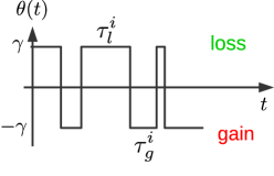
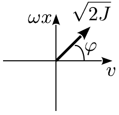
Figure 1: LEFT: The time dependence of the damping function $\theta(t)$. When $\theta=\gamma$ the oscillator undergoes damping (loss) and when $\theta=-\gamma$, the oscillator undergoes anti-damping (gain). The amount of time spent in the gain/loss state before switching is $\tau_{g/l}$. RIGHT: Change of variables.

2.2 Master equation

In order to deal with the stochastic system, we begin by examining the time evolution of $p(x,v,t)$, the probability to find the oscillator in position $x$ with velocity $v=\dot{x}$ at time $t$. To this end we write down the master equation of such a system, keeping in mind that the oscillator can also be in any of the two states $g$ or $l$. Therefore, we have the following system of coupled partial differential equations:

$$[\partial_{t}+v\partial_{x}-\omega^{2}x\partial_{v}]p_{g/l}(x,v,t)\pm 2\gamma\partial_{v}(vp_{g/l}(x,v,t))=\\ \mp(p_{g}(x,v,t)/\tau_{g}-p_{l}(x,v,t)/\tau_{l}),$$ (2)

such that $P_{g/l}(t)=\int_{-\infty}^{\infty}\int_{-\infty}^{\infty}dx\;dv\;p_{g/l}(x,v,t)$ is the probability for the oscillator to be in the gain/loss state at time $t$. Furthermore, the probability is conserved so that $P_{g}(t)+P_{l}(t)=1$. The first term on the left-hand-side of (2) is the deterministic Liouville term, whilst the second one is the gain/loss term that arises from the non-conservative nature of equation (1). The term on the right-hand-side describes the stochastic switching rate of the oscillator between the gain and loss phases.

In as such, one would have to solve the coupled pair of equations in (2) for $p_{g}(x,v,t)$ and $p_{l}(x,v,t)$ in order to completely characterize the stochastic system. However, such a task is extremely heavy and unnecessary for our purpose. As mentioned in the introduction, we are interested in the stability of the stochastic oscillator and a reliable criterion for it. A first simplification arises by noticing that the action-angle variables

$$J=\frac{1}{2}\left(v^{2}+\omega^{2}x^{2}\right)\quad\text{and}\quad\varphi=\arctan(\omega x/v),$$ (3)

are more suitable for handling the master equation. These polar-type coordinates lead to a separation of variables in the master equation in (2) (see A.5 for details). In the optics terminology, $J$ and $\varphi$ correspond respectively to the amplitude and phase while $x$ and $v$ correspond to the quadrature components.

Subsequent Laplace and Mellin transforms allow us to eliminate the time and $J$ derivatives in the resulting master equation. Indeed, these transformations defined respectively as

$$\hat{f}(s)=\int_{0}^{\infty}e^{-st}f(t)\;dt\quad\text{and}\quad\hat{f}(k)=\int_{0}^{\infty}J^{k}f(J)\;dJ.$$ (4)

simplify the master equation into:

$$\left[\frac{d}{d\varphi}(\omega\mp\gamma\sin 2\varphi)+s\mp 4\gamma k\cos^{2}\varphi\right]\hat{p}_{g/l}(k,\varphi,s)=\\ \mp\left(\frac{\hat{p}_{g/l}(k,\varphi,s)}{\tau_{g}}-\frac{\hat{p}_{g/l}(k,\varphi,s)}{\tau_{l}}\right)+\hat{p}_{g/l}(k,\varphi,t_{0}),$$ (5)

where $p_{g/l}(J,\varphi,t_{0})$ is the starting distribution (initial condition), which we assume to be a delta function. Still however, the last form cannot be solved analytically exactly. Nevertheless, essential information can be derived about the asymptotic time limit of the solution (see A.1 and A.2). For large times, we deduce indeed that the variable $\ln J$ follows a normal distribution by showing that any moment of the cumulant expansion of $\ln J$ scales linearly with time (see A.3). As a consequence, the average value $\langle\ln J\rangle$ depends linearly on time and the relative square root variance has the scaling $\sqrt{\langle\delta^{2}\ln J\rangle}/\langle\ln J\rangle\rightarrow 1/\sqrt{t}$ so that asymptotically $\ln J$ becomes a deterministic variable (see A.4). On the other hand, the angle $\varphi$ remains generally distributed over a broad value range. The numerical simulations of the evolution of an ensemble of stochastic oscillators confirm these theoretical results: Figure 2 shows the linear time dependence for the average around which the square root variance remains small in comparison; figure 3 shows the histogram of the distribution of $\ln J$, which converges to a Gaussian in the asymptotic time limit.

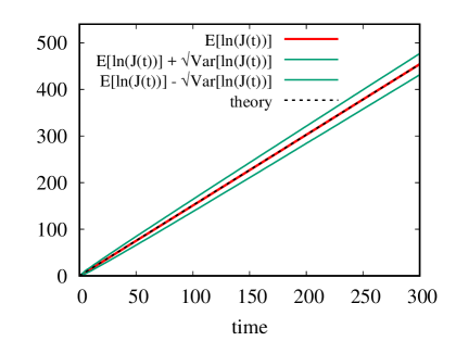
Figure 2: Time evolution of the average of $\bm{\ln J(t)}$ together with its dispersion. In this particular example $\omega=1$, $\gamma=0.9$, $\tau_{g}=5$ and $\tau_{l}=1$. The average is taken over an ensemble of $10^{4}$ oscillators, each with the initial condition $(x_{0},v_{0})=(1,1)$ at $t=0$. The positive slope of $\ln J(t)$ for those particular parameter values implies that the system is unstable in the asymptotic limit. The dashed black line, whose slope was obtained from (6), corresponds to the theoretical result.

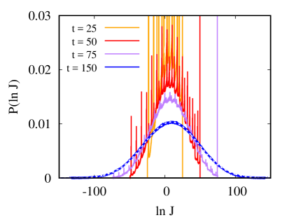
Figure 3: Probability distribution of $\bm{\ln J(t)}$ for $\bm{\tau_{g}=\tau_{l}}$. The different curves show the evolution of the probability distribution over different times $t$. For all the examples shown in the figure, $\omega=1$, $\gamma=0.5$ and $\tau_{g/l}=10$. The white dashed line is the Gaussian fit to the simulation result in blue. The fit parameters correspond to $\mu$ = 9.1 for the average and $\sigma$ = 38.8 for the standard deviation . An ensemble of $10^{8}$ oscillators was used to create both distributions, each oscillator having the initial condition $(x_{0},v_{0})=(1,1)$ at $t=0$.

2.3 The stability criterion

In order to assess the stability of the dynamics of the stochastic oscillator, we can use the following results established in A.4. If the asymptotic marginal distribution $P_{g/l}(\varphi)=\lim_{t\rightarrow\infty}\int_{0}^{\infty}p_{g/l}(J,\varphi,t)\;dJ$ exists, then the asymptotic constant $\eta$ associated to the linear evolution of the first moment is given by:

$$\eta=\lim_{t\rightarrow\infty}\frac{d}{dt}\langle\ln J\rangle(t)=\frac{\int_{-\pi/2}^{\pi/2}4\gamma\cos^{2}\varphi\;\left(P_{g}(\varphi)-P_{l}(\varphi)\right)d\varphi}{\int_{-\pi/2}^{\pi/2}\left(P_{g}(\varphi)+P_{l}(\varphi)\right)d\varphi},$$ (6)

This real-valued constant is the basis of the stability criterion that we shall employ in the next section. A positive $\eta$ corresponds to a diverging first moment of $\ln J$ implying that the system is unstable while a negative $\eta$ corresponds to a stable system. In order to apply the stability criterion defined in (6), we need to determine $P_{g}(\varphi)$ and $P_{l}(\varphi)$ asymptotically.

3 Stability results of the stochastic oscillator in the asymptotic limit

3.1 Simulated results compared with the theory

We used numerical simulations of the evolution of an ensemble of stochastic oscillators from which we extract the asymptotic first moment of $\ln J(t)$ and thus determine $\eta$. The results are plotted in figure 4. The green area corresponds to negative values of the slope of the ensemble average of $\ln J$ whilst the red corresponds to positive ones. For $\gamma<\omega$, the two regions are separated by the line of symmetry $\tau_{g}=\tau_{l}$. This result corresponds to what one might expect - if the amount of time spent in the gain state is on average longer than in the loss state, then the average value of the energy diverges over time. On the other hand, if the system on average spends more time in a loss state, then its average energy decays to zero over time. What comes as a surprise is that when $\gamma>\omega$ the system energy can diverge even when $\tau_{l}>\tau_{g}$. In order to see this better it is worth theoretically studying the dependence of $\eta$ in terms of $\gamma$.

In the limit of large $\tau_{g}$ and $\tau_{l}$, we calculate explicitly the formula (6) using the expressions for $P_{g/l}(\varphi)$ derived in A.5 and A.6 to obtain the simple analytic forms:

$$\eta=\left\{\begin{aligned} &2\gamma\frac{\tau_{g}-\tau_{l}}{\tau_{g}+\tau_{l}},&\quad\gamma<\omega\\ &2\gamma\left(\frac{\tau_{g}-\tau_{l}}{\tau_{g}+\tau_{l}}+\sqrt{1-\left(\omega/\gamma\right)^{2}}\right),&\quad\gamma>\omega.\end{aligned}\right.$$ (7)

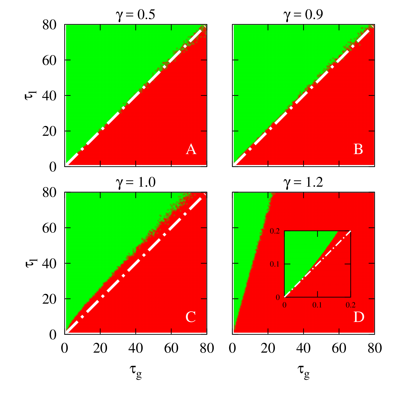
Figure 4: Stability of the stochastic oscillator. The figure shows the stability analysis done using numerical simulations according to the criterion defined in (6). The green color indicates the stable region, where the average of $\ln J$ is negative and the red color indicates the unstable region, where it is positive. Panels A and B: In this case $\gamma<\omega$. It can be seen that the line of symmetry $\tau_{g}=\tau_{l}$ separates the stable region from the unstable. Panel C: This is the critical case where $\omega=\gamma$. Since the system is not in the asymptotic regime, the symmetry line $\tau_{g}=\tau_{l}$ does not separate the two regions perfectly. Panel D: An example of the case where $\gamma>\omega$. It shows that the symmetry line $\tau_{g}=\tau_{l}$ is well below the line that separates the two regions. Consequently there exist cases where $\tau_{g}$ is well below $\tau_{l}$ and yet the system is still unstable. The inset shows that for small values of $\tau_{g}$ and $\tau_{l}$ symmetry is regained, as discussed at the end of A.6. In all four cases an ensemble of 1000 oscillators that evolved up to $t=300$ were used, each oscillator having the initial condition $(x_{0},v_{0})=(1,1)$ at $t=0$.

From (7), a necessary condition for stability is that $\tau_{g}<\tau_{l}$, independent of the values of $\omega$ and $\gamma$. Furthermore for $\gamma<\omega$, the asymptotic expression is in good agreement with the simulation results, whereby the oscillator is at the edge of stability for $\tau_{g}=\tau_{l}$. Asymptotically, the energy logarithm $\ln J$ can be considered as a deterministic quantity, which does not decay nor diverge when there is a perfect balance between gain and loss, when $\tau_{g}=\tau_{l}$. On the other hand, when $\gamma>\omega$ a gain-loss balance ($\tau_{g}=\tau_{l}$) does not induce stability in the system. On the contrary, the system can remain active with a growing or constant energy even when the loss states dominate over the gain states, i.e. when $\tau_{l}>\tau_{g}$. This is illustrated by the green curve in figure 5; there is a value of $\gamma$ above which the system’s energy diverges no matter how large $\tau_{l}$ becomes compared to $\tau_{g}$.

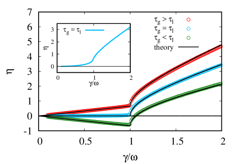
Figure 5: Stability analysis of the stochastic oscillator as a function of $\bm{\gamma}$. The colored circles correspond to values of the stability parameter $\eta$ in the large $\tau_{l},\tau_{g}$ limit, determined numerically from simulations. RED: Predominant gain where $\tau_{g}=100$ and $\tau_{l}=50$. BLUE: Balanced state where $\tau_{g}=\tau_{l}=50$. GREEN: Predominant loss where $\tau_{g}=50$ and $\tau_{l}=100$. The BLACK curves correspond to the theoretical result displayed in (7). The INSET shows the dependence of $\eta$ on $\gamma$ in the intermediate $\tau_{g},\tau_{l}$ limit. The blue curve is the result of a simulation with $\tau_{l}=\tau_{g}=5$. In this limit, symmetry is broken even for $\gamma<\omega$. In all simulations an ensemble of $10^{5}$ oscillators evolving up to $t=300$ were used, each oscillator having the initial condition $(x_{0},v_{0})=(1,1)$ at $t=0$.

3.2 The effective transition to a broken $\mathcal{PT}$ symmetry phase

We can more precisely formalize what was said above by investigating further the system by analyzing the symmetry properties of the probability density functions $p_{g}$ and $p_{l}$. We define the space reflection, or parity operator $\mathcal{P}$ as the exchange between the gain and loss probability densities of $\varphi$. In other words, $\mathcal{P}$ has the effect of swapping $g$ and $l$ so that we have the exchange $P_{g}\leftrightarrow P_{l}$. A similar definition is encountered in [2, 3] where for simplicity the real space is represented by a two-valued position (let us say $\pm 1$) and the parity operation represent the exchange between $+1$ and $-1$. This redefined operation has been used as a swap operation between two quantum states and subsequently for the swap between the gain and loss states in [14]. We can also include the time-reversal operation $\mathcal{T}$, where $t\rightarrow-t$, $v\rightarrow-v$ and $x\rightarrow x$ so that $\varphi\rightarrow-\varphi$. If we apply both operations at the same time, the distributions $P_{l}(\varphi)$ and $P_{g}(\varphi)$ remain invariant so that the ${\cal PT}$ symmetry is fulfilled.

The ensemble of stochastic oscillators is effectively $\mathcal{PT}$-symmetric in the so-called underdamped regime when $\gamma<\omega$ and under the condition that $\tau_{g}=\tau_{l}$, although neither the stochastic equation (1) nor the master equation (2) obey such a symmetry. Indeed, the phase probability densities $P_{g}(\varphi)$ and $P_{l}(\varphi)$ obtained by simulation and represented in the first graph of figure 6 have a mirror symmetry with respect to the origin ($\varphi\rightarrow-\varphi$). For comparison, the analytic expression for $P_{g/l}(\varphi)$ is obtained by solving the master equation in (2) in the large time limit (numerical integration and asymptotic expression in the large $\tau_{g/l}$ limit in A.6).

However, this symmetry is only effective if we compare values of $\ln J$ up to its square root variance given that $\ln J$ keeps diffusing normally. But if we compare the square root variance relatively to any non trivial average of $\ln J$, it shrinks to zero in the large time limit. Therefore these considerations have only a strict sense in the asymptotic limit viewed here as the analog of the thermodynamic limit where the concept of a large particle number of a thermodynamic system is replaced by one of large time, and where the so-called normal quantities are the average and the variance of $\ln J$ that both scale linearly with time (see A.3 and A.4).

The mirror symmetry of $P_{g/l}(\varphi)$ is maintained only for $\gamma<\omega$. Once this condition is no longer satisfied, the distribution of $\varphi$ initially broadly distributed in the symmetric case condenses by forming two delta-like peaks. It is in this sense that the system becomes deterministic once $\gamma$ is greater than $\omega$. At the same time, however, the mirror symmetry of the probability densities is broken as can be seen in the second graph of figure 6 leading to a ${\cal PT}$-symmetry violation. In the limit of large $\tau_{g}$ and $\tau_{l}$ we are able to calculate a simple expression that determines the values $\varphi_{g/l}$ at which the two peaks in $P_{g/l}(\varphi)$ occur (see A.6 for details):

$$\tan\varphi_{g/l}=\omega\frac{x_{g/l}}{v_{g/l}}=\pm\frac{\gamma}{\omega}-\sqrt{\left(\frac{\gamma}{\omega}\right)^{2}-1}.$$ (8)

The new ”phase” obtained is ordered in the sense that it corresponds to a ratio locking of the velocity over the position with different fixed values for the gain state and the loss state. This result may also been obtained more intuitively by noticing that for $\gamma\geq\omega$ the oscillator is damped with no oscillations. It corresponds to the overdamped regime as opposed to the underdamped regime where oscillations persist. We can indeed solve (1) using the ansatz $x(t)=e^{\lambda t}x(0)$ and find that $\lambda=\pm\gamma\pm\sqrt{\gamma^{2}-\omega^{2}}$ is real only in the overdamped regime. Hence, in the large time limit only one eigenvalue is dominant and therefore using $\omega x(t)/v(t)=\omega/\lambda$ for the dominant eigenvalue, we recover (8) accordingly. Such a relation could not have been used in the underdamped regime since the phase of oscillations would have randomized the trajectories.

We interpret this observation as a phase transition from a disordered state to an ordered state with symmetry breaking in analogy to what happens in phase transition phenomena in thermodynamics. It can therefore be concluded that the ${\cal PT}$-symmetry breaking occurs at the point of critical damping ($\gamma=\omega$). In analogy to the Ising model [18], we start from a symmetric state with no ordering above a critical point, the broad angle distribution in our case (or the spin distribution in the magnet), and go towards a broken symmetry state with a well defined order with two possible opposite angle values e.g. ratio locking (or a well defined value of spin).

We end this section by adding that the symmetry breaking established in the limit of large $\tau_{l,g}$ is essentially valid also in the intermediate regime, despite a little bias ($\tau_{l}>\tau_{g}$) for $\gamma$ around $\omega$ shown in panel C of figure 4 and in the inset of figure 5. The symmetry is totally restored, however, in the limit of small $\tau_{l,g}$ whatever the value of $\gamma$ as can been seen from the inset in figure 4.

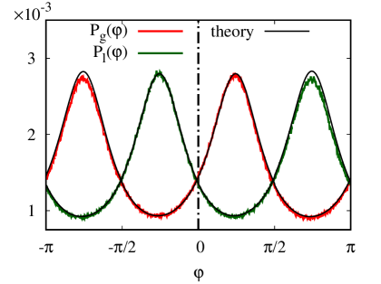
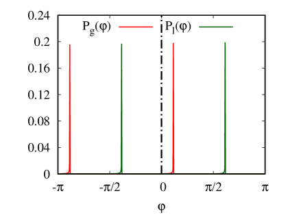
Figure 6: The distribution of the phases $\bm{P_{g}(\varphi)}$ and $\bm{P_{l}(\varphi)}$. TOP: The system exhibits mirror symmetry and dispersed phases in the case where $\gamma<\omega$ and $\tau_{g}=\tau_{L}$. In this example $\gamma=0.5$, $\omega=1$ and $\tau_{g/l}=20$. An ensemble of $10^{6}$ oscillators was allowed to evolve up to $t=1500$. The black curve corresponds to the numerical solution of the analytical result in (46). BOTTOM: The symmetry is broken when $\gamma>\omega$ and the phases become localized. When $\gamma$ becomes larger than $\omega$ a transition occurs from a disordered to an ordered phase with a velocity-position ratio locking. In this example $\gamma=0.5$, $\omega=1.5$ and $\tau_{g/l}=10$. An ensemble of $10^{6}$ oscillators was allowed to evolve up to $t=300$, each oscillator having the initial condition $(x_{0},v_{0})=(1,1)$ at $t=0$.

4 Stability of the first moments

4.1 Dynamic equations for the position and velocity average

The stability criterion obtained in the previous section does not mean that all physical quantities of interest are stable. This statement can be illustrated by considering the evolution of the first moments of $p_{g}$ and $p_{l}$. The fact that $\ln J$ is stable does not necessarily mean that averages involving position and speed average are stable. Indeed, if $f(\varphi)$ is a function to average, from the Feymann-Gibbs inequality, we deduce:

$$\langle\alpha f(\varphi)\ln J\rangle\leq\ln\langle J^{\alpha}\exp(\alpha f(\varphi))\rangle$$ (9)

On the contrary, the stability of position and velocity averages implies stability of $\ln J$. Therefore, there exist additional requirements that enhance the stability of the stochastic oscillators, adding to the richness of their dynamics.

By multiplying both equations in (2) by $x$ and $v$ and integrating over the entire space and all the velocities, we obtain a system of coupled first order differential equations:

$$\frac{d}{dt}\langle x\rangle_{l} =\langle v\rangle_{l}-\frac{\langle x\rangle_{l}}{\tau_{l}}+\frac{\langle x\rangle_{g}}{\tau_{g}}$$ (10)

$$\frac{d}{dt}\langle v\rangle_{l} =-\omega^{2}\langle x\rangle_{l}-2\gamma\langle v\rangle_{l}-\frac{\langle v\rangle_{l}}{\tau_{l}}+\frac{\langle v\rangle_{g}}{\tau_{g}}$$

$$\frac{d}{dt}\langle x\rangle_{g} =\langle v\rangle_{g}+\frac{\langle x\rangle_{l}}{\tau_{l}}-\frac{\langle x\rangle_{g}}{\tau_{g}}$$

$$\frac{d}{dt}\langle v\rangle_{g} =-\omega^{2}\langle x\rangle_{g}+2\gamma\langle v\rangle_{g}+\frac{\langle v\rangle_{l}}{\tau_{l}}-\frac{\langle v\rangle_{g}}{\tau_{g}}$$

where

$$\langle x\rangle_{g/l}=\int_{-\infty}^{\infty}dx\int_{-\infty}^{\infty}dv\;x\;p_{g/l}(x,v,t)\quad\text{and}\quad\langle v\rangle_{g/l}=\int_{-\infty}^{\infty}dx\int_{-\infty}^{\infty}dv\;v\;p_{g/l}(x,v,t).$$ (11)

The linear dynamical system described here is of the form $\bm{\dot{z}=M\cdot z}$ and therefore an asymptotically stable condition is verified when all of the real parts of the roots of the characteristic polynomial associated with $\bm{M}$ are negative. It is straightforward to determine the four eigenvalues which we shall denote as $\bm{\lambda}=(\lambda_{1},\lambda_{2},\lambda_{3},\lambda_{4})$ (see B for details). Consequently the stability is also asymptotic in time.

In a way similar to what was presented in the previous sections, the dynamical system governing the first moments can be separated into two regimes, namely, the case where $\gamma<\omega$ and $\gamma>\omega$. We proceed by examining the stability conditions for such a system and without loss of generality we assume that $\omega=1$. We show that in this case also, depending on the value of $\gamma$, it is possible to have a situation in which the average quantities we studied diverge even though the system, on average, spends more time in the loss state than in the gain state. In contrast to the results obtained regarding the stability of $\ln J$ in the previous section, the average values in (10) diverge when $\tau_{l}=\tau_{g}$ since there exists at least one eigenvalue that is positive for any combination of the other parameters (see B for details).

4.2 Underdamped case: $\gamma<\omega$

In this case, all four eigenvalues $\lambda_{i}$ are complex and they come in conjugate pairs (see B). The real parts of two of them are equal, $Re\lambda_{1}=Re\lambda_{2}$, and negative for all combinations of $(\tau_{g}$,$\tau_{l})$ whilst the real parts of the other two, which are also equal ($Re\lambda_{3}=Re\lambda_{4}$), can be either positive or negative. Since the imaginary parts of all four eigenvalues are always non-zero, all the solutions of the system (10) are oscillatory, whether they decay or grow, for any value of $\tau_{l}$ and $\tau_{g}$. For a fixed $\gamma$ we numerically determine the regions in the $\tau_{l}-\tau_{g}$ parameter space for which every eigenvalue of the system has a negative real part. This corresponds to the stable region and is indicated in green in panels A and B of figure 7. Moreover, the relation $\lim_{\tau_{l}\rightarrow\infty}\lambda_{i}=\gamma-1/\tau_{g}$ for $i=3,4$ derived using 58 imposes the critical value $\tau_{g}^{*}=1/\gamma$ beyond which stability is never attained no matter how large the value of $\tau_{l}$ is.

4.3 Overdamped case: $\gamma\geq\omega$

Once the stochastic oscillator is overdamped, more of the eigenvalues can attain positive real parts, rendering the dynamics more elaborate. In particular, in contrast to the underdamped case, $Re\lambda_{2}$ can also be positive, depending on the values of $\tau_{g}$ and $\tau_{l}$. Nevertheless, the stability does not differ qualitatively from the underdamped case. The boundary that separates the stable from the unstable region continues to shift towards lower values of $\tau_{g}$ when $\gamma$ increases further. Another interesting property deduced from the eigenvalues is that in the overdamped case there exist oscillatory solutions to (10) in contrast to the simple damped harmonic oscillator that is monotonically damped under those conditions. These oscillations occur when at least one of the eigenvalues has a non-zero imaginary part. This is the case for values of $(\tau_{l},\tau_{g})$ for which $|Im\lambda_{1}|+|Im\lambda_{2}|+|Im\lambda_{3}|+|Im\lambda_{4}|\neq 0$. These results are presented in panels C and D of figure 7 where, although the monotonic motion is predominant in the overdamped case, there persists a region in the $\tau_{g}-\tau_{l}$ plane for which the solutions are oscillatory.

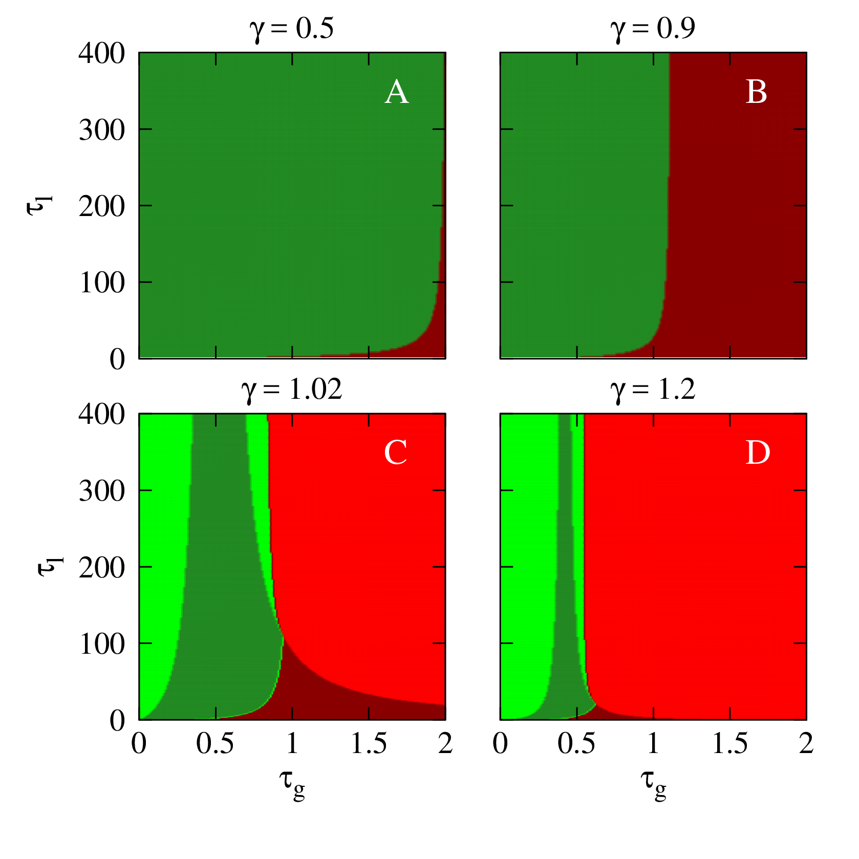
Figure 7: Stability analysis for the evolution of the first moments. The stable regions in parameter space for which all four eigenvalues have negative real parts are colored green while the unstable regions are in red. Each panel in the figure was made by evaluating directly the real parts of the eigenvalues in (58) belonging to the dynamical system (10). In all cases $\omega=1$ and each oscillator was with the initial condition $(x_{0},v_{0})=(1,1)$ at $t=0$. In the underdamped regime, the comparison between PANELS A and B show a stable region that decreases with growing $\gamma$. PANELS C and D show two examples of the overdamped regime for different values of $\gamma$. The dark green and dark red colors denote the set of values $(\tau_{g},\tau_{l})$ for which the solutions of the dynamical system are oscillatory (in the underdamped regime, all solutions are oscillatory). In this case also, both the stable and oscillatory regions diminish in size with increasing $\gamma$.

5 Full time analysis at zero frequency

Until now, we have analyzed the asymptotic behavior of the oscillator in the large time limit and also the first moment of the position and the velocity. For the sake of completeness, it remains in principle to discuss about the short and intermediate time regimes and the stability of the higher order moments. A full analysis is beyond the scope of this paper but we can address the particular case of $\omega=0$, so that the problem reduces to the simpler dynamical equation in which the position coordinate is eliminated:

$$\frac{dv(t)}{dt}=\pm 2\gamma v(t)$$ (12)

This dynamical equation describes the evolution of a wave function that is amplified or undergoes loss randomly. A similar study where the frequency takes randomly two possible values has been shown useful in the context of superconducting qubits [19]. This type of model has already been used to determine the first passage time at which, for instance, the speed exceeds a critical value [20, 21, 22, 23]. The interest here is to illustrate how the exact solution complements the results obtained so far.

We start from the initial condition: $p_{g/l}(v,t=0)=p_{g/l}\delta(v-v_{0})$ and solve this equation using the variable change: $r=\ln(v/v_{0})/(2\gamma)$ (see C). The short time analysis differs from the asymptotic analysis because the distribution is not normal anymore. If we start with a well defined speed $v_{0}$ and study its subsequent evolution for short time ($t\ll\tau_{g/l}$), we obtain the spread of the velocity distribution but confined within a cone:

$$p_{g/l}(v,t\simeq 0)=\frac{1}{v}\left[p_{g/l}\delta(r-t)(1-\frac{t}{\tau_{g/l}})+\frac{p_{l/g}}{2\tau_{l/g}}1^{+}(t^{2}-r^{2})\right],$$ (13)

where $1^{+}(x)$ is the Heaviside function. The short time behavior is characterized by a propagation of a delta distribution along this cone inside which the probability densities develop. In the opposite case for large time ($t\gg\tau_{g/l}$), we find a normal distribution for the variable $r$ with average and variance:

$$\langle\ln\left(\frac{v(t)}{v_{0}}\right)\rangle=\frac{\tau_{g}-\tau_{l}}{\tau_{g}+\tau_{l}}2\gamma t,\quad\sigma^{2}(t)=\langle\delta^{2}\ln\left(\frac{v(t)}{v_{0}}\right)\rangle=\frac{(2\gamma)^{2}8\tau_{l}^{2}\tau_{g}^{2}}{(\tau_{g}+\tau_{l})^{3}}t$$ (14)

Thus, the stability of the average is satisfied for $\tau_{l}\geq\tau_{g}$ in contrast to the previous statements in (7), which always predict instability. The apparent contradiction is resolved by remembering that according to (9) the stability of $r$ does not imply the stability of any moment of the velocity and/or any moment of the position. Indeed for the $n^{th}$ moment, we determine the following more restrictive stability criterion:

$$n\leq\frac{\tau_{l}-\tau_{g}}{2\gamma\tau_{g}\tau_{l}}$$ (15)

Therefore, there always exists an order $n$ above which the stability criterion is not satisfied in accordance with the variance in (14), which always increases. However, if we restrict to the $v$ variable only without the position $x$ then the simplified system becomes effectively always ${\cal PT}$ symmetric when $\tau_{l}=\tau_{g}$.

6 Conclusions and perspectives

We have studied the dynamic evolution of stochastic oscillators subject to dichotomous noise made of alternating gain and loss states random in time and we have unveiled an intimate connection of this non conservative system with ${\cal PT}$ symmetry. We established a useful criterion that fixes the boundary line between a stable regime with a likely decaying amplitude and an unstable regime with a likely growing one. Although the oscillator evolution becomes more stochastic with time, it is nevertheless possible to effectively define the useful concept of ${\cal PT}$ symmetry in the asymptotic time limit. In other words, despite the breaking of time reversal invariance due to noise, the oscillator can still remain resilient so as to preserve at least the ${\cal PT}$ symmetry. Application of this invariance property allows to distinguish between different regimes or phases: a) an underdamped regime (or weakly damping-amplifying oscillator ) for which the boundary lines between stable and unstable regions satisfy this symmetry; b) an overdamped regime (or strongly damping-amplifying oscillator) for which this boundary line becomes asymmetric. We interpret these results in analogy to thermodynamics as a phase transition from a symmetric disordered state consisting of a broad distribution to an ordered state with a restricted distribution imposing a ratio locking of the position over the velocity separately for both the gain and loss states.

To complete the panorama, we also examined the time evolution of the position and velocity averages of the oscillator. We showed that the stability of the oscillator does not necessarily imply bounded dynamics of these averages. It appears indeed that the stability diagrams are more elaborate, illustrating the much richer structure of this apparently very simple system. For instance, despite the absence of oscillations in the deterministic case, in the overdamped regime the presence of a random gain can re-stimulate them. Higher order moment analysis together with a study of the short and intermediate time limits confirm this broad range of different regimes with different physics such as the cone-like propagation of the velocity distribution.

The formalism developed here in the particular case of a stochastic oscillator is quite general and may be applied to other situations where dichotomous noise is present such as the stabilization of light propagation in metamaterials and optical fibres with random regions of asymmetric active and passive media [7].

Appendix A Asymptotic solution of the master equation

A.1 Dominant eigenvalue

After reducing the master equation (2) to a pair of coupled ordinary differential equations by means of integral transforms, we write the master equation (5) under a matrix form with $p_{g/l}(J,\varphi,t_{0})$ as the initial distribution:

$$\mathcal{M}\cdot\hat{p}=-s\hat{p}+\hat{p}(k,\varphi,t_{0}),$$ (16)

where

$$\mathcal{M}=\mathcal{M}^{(0)}+k\mathcal{M}^{(1)}=\left[\begin{pmatrix}\mathcal{L}_{g}^{(0)}&-1/\tau_{l}\\ -1/\tau_{g}&\mathcal{L}_{l}^{(0)}\end{pmatrix}+k\begin{pmatrix}-4\gamma\cos^{2}\varphi&0\\ 0&4\gamma\cos^{2}\varphi\end{pmatrix}\right]$$ (17)

in which

$$\mathcal{L}^{(0)}_{g/l}=\frac{d}{d\varphi}(\omega\mp\gamma\sin 2\varphi)+\frac{1}{\tau_{g/l}}.$$ (18)

and where

$$\hat{p}=\left(\begin{array}[]{c}\hat{p}_{g}\\ \hat{p}_{l}\end{array}\right)\quad\quad\hat{p}(k,\varphi,t_{0})=\left(\begin{array}[]{c}\hat{p}_{g}(k,\varphi,t_{0})\\ \hat{p}_{l}(k,\varphi,t_{0})\end{array}\right).$$ (19)

Note that because of the inversion symmetry $x\rightarrow-x$ and $v\rightarrow-v$, the stochastic oscillator is invariant under the transformation $\varphi\rightarrow\varphi+\pi$. Therefore, we can restrict the angle to the interval $\varphi\in]-\pi/2,\pi/2]$. Writing the solution $\hat{p}(k,\varphi,s)$ as a linear combination of the eigenfunctions $\hat{p}_{i}(k,\varphi)$ of $\mathcal{M}$ with eigenvalue $-s_{i}$ we obtain

$$\hat{p}(k,\varphi,s)=\sum_{i}c_{i}(s)\hat{p}_{i}(k,\varphi).$$ (20)

In that case, the master equation becomes

$$\sum_{i}(s+s_{i})c_{i}(s)\hat{p}_{i}(k,\varphi)=\hat{p}(k,\varphi,t_{0}).$$ (21)

Multiplying from the left with the eigenfunction $\tilde{p}_{j}^{\dagger}(k,\varphi)$ of the adjoint problem with eigenvalue $s_{j}$ and using the bi-orthogonality property

$$\int_{-\pi/2}^{\pi/2}\tilde{p}_{i}^{\dagger}\cdot\hat{p}_{j}\;d\varphi=0\quad\quad i\not=j,$$ (22)

we obtain

$$c_{j}(s)=\frac{\int_{-\pi/2}^{\pi/2}\tilde{p}_{j}^{\dagger}(k,\varphi)\cdot\hat{p}(k,\varphi,t_{0})\;d\varphi}{(s+s_{j})\int_{-\pi/2}^{\pi/2}\tilde{p}_{j}^{\dagger}(k,\varphi)\cdot\hat{p}_{j}(k,\varphi)\;d\varphi}=\frac{A_{j}(k)}{s+s_{j}}.$$ (23)

Taking the inverse Laplace transform, we arrive at

$$c_{j}(t)=\exp\left[-s_{j}t\right]A_{j}(k).$$ (24)

Therefore, the inverse Laplace transform of (20) gives

$$\hat{p}(k,\varphi,t)=\sum_{i}\exp[-s_{j}t]A_{j}(k)\hat{p}_{i}(k,\varphi).$$ (25)

In the asymptotic time limit where $t\rightarrow\infty$, assuming that $s_{0}$ is the dominant eigenvalue in the sense that the real component ${\rm Re}\,s_{0}$ has the lowest value among all eigenvalues, we simplify the dynamics into:

$$\hat{p}(k,\varphi,t\rightarrow\infty)=\exp[-s_{0}t]A_{0}(k)\hat{p}_{0}(k,\varphi).$$ (26)

A.2 Perturbation theory

We progress further using the perturbation expansion applied to the eigenvalue problem:

$$\mathcal{M}\cdot\hat{p}_{i}=(\mathcal{M}^{(0)}+k\mathcal{M}^{(1)})\cdot\hat{p}_{i}=-s_{i}\hat{p}_{i}$$ (27)

where $\hat{p}_{i}=(\hat{p}_{i,g}\;\hat{p}_{i,l})^{T}$ is a spinor and where the matrix operator $\mathcal{M}$ is the sum of the principle part $\mathcal{M}^{(0)}$ and a perturbation part $\mathcal{M}^{(1)}$ whose matrix elements can be deduced directly from (17). In order to solve the eigenvalue problem for the operator (17), we expand the $i^{th}$ eigenvalue, $s_{i}$, of the operator $\mathcal{M}$ in powers of the perturbation parameter $k$ so that

$$s_{i}=s_{i}^{(0)}+ks_{i}^{(1)}+k^{2}s_{i}^{(2)}/2!+\ldots\;.$$ (28)

In the leading order, $s_{i}^{(0)}$ is equal to the eigenvalue of the unperturbed operator $\mathcal{M}^{(0)}$ while, in the first order, we find using (22) the first correction:

$$s_{i}^{(1)}=-\frac{\int_{-\pi/2}^{\pi/2}\tilde{p}_{i}^{\dagger(0)}\cdot\mathcal{M}^{(1)}\cdot\hat{p}_{i}^{(0)}d\varphi}{\int_{-\pi/2}^{\pi/2}\tilde{p}_{i}^{\dagger(0)}\cdot\hat{p}_{i}^{(0)}d\varphi},$$ (29)

where $\hat{p}_{i}^{(0)}=(\hat{p}_{i,g}^{(0)}\;\hat{p}_{i,l}^{(0)})^{T}$ is the solution to the unperturbed eigenvalue problem ($i^{(th)}$ eigenvector) that involves only $\mathcal{M}^{(0)}$. Since the operator is not self-adjoint, we must use $\tilde{p}_{i}^{(0)}$, which is the solution to the zeroth order adjoint problem defined by

$$\mathcal{M}^{\dagger(0)}\cdot\tilde{p}^{(0)}_{i}=\begin{pmatrix}\mathcal{L}^{\dagger(0)}_{g}&-1/\tau_{g}\\ -1/\tau_{l}&\mathcal{L}^{\dagger(0)}_{l}\end{pmatrix}\cdot\left(\begin{array}[]{c}\tilde{p}_{i,g}^{(0)}\\ \tilde{p}_{i,l}^{(0)}\end{array}\right)=-s^{(0)}_{i}\left(\begin{array}[]{c}\tilde{p}_{i,g}^{(0)}\\ \tilde{p}_{i,l}^{(0)}\end{array}\right),$$ (30)

where the adjoint operator has the form

$$\mathcal{L}_{g/l}^{\dagger(0)}=-(\omega\mp\gamma\sin 2\varphi)\frac{d}{d\varphi}+\frac{1}{\tau_{g/l}}.$$ (31)

It is easily verified that in the unperturbed case, the adjoint problem has the trivial solution $\tilde{p}_{0}^{(0)}=(1\;1)^{T}$ with the eigenvalue $s_{0}^{(0)}=0$. This trivial eigenvalue is the most dominant because an eigenvalue with a real positive value would lead to a probability that is not conserved in time. In fact, this eigenvalue is precisely associated to the probability conservation. Therefore, up to first order in $k$, the dominant solution of the eigenvalue problem (29) is rewritten using (17) more simply as:

$$s_{0}=s_{0}^{(0)}+ks_{0}^{(1)}=-k\frac{\int_{-\pi/2}^{\pi/2}4\gamma\cos^{2}\varphi\;\left(\hat{p}_{g}(0,\varphi,0)-\hat{p}_{l}(0,\varphi,0)\right)d\varphi}{\int_{-\pi/2}^{\pi/2}\left(\hat{p}_{g}(0,\varphi,0)+\hat{p}_{l}(0,\varphi,0)\right)d\varphi}.$$ (32)

A.3 Evolution of the central moments of $\ln J$

We start with the Mellin transform shown in (4) and write it down as a characteristic function of the total probability for the variable $\ln J$:

$$M_{\ln J}(k,t) = \int_{-\pi/2}^{\pi/2}\!\!\hat{p}_{g}(k,\varphi,t)+\hat{p}_{l}(k,\varphi,t)\;d\varphi$$ (33)

$$= \int_{-\pi/2}^{\pi/2}\int_{0}^{\infty}\!\!e^{k\ln J}(p_{g}(J,\varphi,t)+p_{l}(J,\varphi,t))\;dJd\varphi.$$

If we write down the exponential as a power series and integrate over $\varphi$, we obtain an expression with the moment generating function of $\ln J$ on the right-hand-side:

$$M_{\ln J}(k,t)=\sum_{n=0}^{\infty}\frac{k^{n}}{n!}\langle(\ln J)^{n}\rangle(t).$$ (34)

Therefore, in order to obtain the evolution in time of the $n^{\rm th}$ central moment of $\ln J$, we take the $n^{\rm th}$ derivative of the logarithm of the moment-generating function above (i.e. derive the cumulant generating function) with respect to $k$ [24],

$$\langle(\ln J-\langle\ln J\rangle)^{n}\rangle=\left.\frac{d^{n}}{dk^{n}}\right|_{k=0}\ln M_{\ln J}(k,t).$$ (35)

According to perturbation theory, we can expand the dominant eigenvalue $s_{0}$ in powers of $k$. By substituting this expansion into the Mellin-transformed probability distribution obtained in the asymptotic time limit in equation (26) we obtain:

$$\ln M_{\ln J}(k,t) \stackrel{{\scriptstyle t\rightarrow\infty}}{{=}} -s_{0}^{(0)}t-ks_{0}^{(1)}t-k^{2}s_{0}^{(2)}t/2!-\ldots+\ln A_{0}(k)$$ (36)

$$+ \ln\left(\int_{-\pi/2}^{\pi/2}\hat{p}_{0,g}(k,\varphi)+\hat{p}_{0,l}(k,\varphi)\;d\varphi\right).$$

Finally, for the $n^{th}$ central moment with respect to the quantity $\ln J$, we identify simply in the asymptotic time limit:

$$\langle(\ln J-\langle\ln J\rangle)^{n}\rangle\stackrel{{\scriptstyle t\rightarrow\infty}}{{=}}-s_{0}^{(n)}t.$$ (37)

where $s_{0}^{(n)}$ is the $n^{th}$ expansion coefficient in $k$ of the eigenvalue $s_{0}=\sum_{n=0}^{\infty}{s_{0}^{(n)}k^{n}}/{n!}$. Note that the asymptotic result does not depend anymore on the initial condition through $A_{0}(k)$.

A.4 Stability criterion

As already mentioned in A.2, the master equation can be treated as a perturbed eigenvalue problem with $k$ as the perturbation parameter and $s$ as the eigenvalue to be determined. Given that the dominant eigenvalue for the unperturbed problem is $s^{(0)}_{0}=0$ (see A.1), so that $s_{0}=ks_{0}^{(1)}$ up to first order, we can substitute the time derivative of the first moment in (37) into (32) to obtain finally the stability criterion defined in section 2.3:

$$\frac{d}{dt}\langle\ln J\rangle(t)\stackrel{{\scriptstyle t\rightarrow\infty}}{{=}}-s_{0}^{(1)}=\frac{\int_{-\pi/2}^{\pi/2}4\gamma\cos^{2}\varphi\;\left(\hat{p}_{g}(0,\varphi,0)-\hat{p}_{l}(0,\varphi,0)\right)d\varphi}{\int_{-\pi/2}^{\pi/2}\left(\hat{p}_{g}(0,\varphi,0)+\hat{p}_{l}(0,\varphi,0)\right)d\varphi}.$$ (38)

The linear growth of the first two central moments means that the relative square root variance or the square root variance-to-mean ratio shrinks to zero asymptotically, i.e.,

$$\frac{\sqrt{Var[\ln J]}}{\langle\ln J\rangle}\stackrel{{\scriptstyle t\rightarrow\infty}}{{=}}\frac{\sqrt{s_{0}^{(2)}}}{s_{0}^{(1)}}\frac{1}{\sqrt{t}}\rightarrow 0,$$ (39)

provided $\langle\ln J\rangle\not=0$. This result leads us to conclude that $\ln J$ is in general a well defined statistical variable and can be viewed as a deterministic one in the asymptotic sense (see figure 2). Strictly speaking, only the case $\langle\ln J\rangle=0$ has to be considered non deterministic but distributed within the interval of the square root variance.

A.5 Solution to the unperturbed eigenvalue problem

Setting $s=k=0$ in (5), we notice that the functions:

$$X_{1}\equiv\omega(\hat{p}_{g}+\hat{p}_{l})-\gamma\sin(2\phi)(\hat{p}_{g}-\hat{p}_{l})$$ (40)

and

$$X_{2}\equiv-\gamma\sin(2\phi)(\hat{p}_{g}+\hat{p}_{l})+\omega(\hat{p}_{g}-\hat{p}_{l}).$$ (41)

satisfy a much simpler system of linear first order differential equations:

$$\frac{dX_{1}}{d\varphi}=0\quad\text{and}\quad\frac{dX_{2}}{d\varphi}+A_{+}(\varphi)X_{2}=-A_{-}(\varphi)X_{1},$$ (42)

where,

$$A_{\pm}(\varphi)=\dfrac{\tau_{l}(\omega+\gamma\sin 2\varphi)\pm\tau_{g}(\omega-\gamma\sin 2\varphi)}{\tau_{g}\tau_{l}(\omega^{2}-\gamma^{2}\sin^{2}(2\varphi))}.$$ (43)

The first equation, for $X_{1}$, is trivial whose solution is a constant. The second equation, for $X_{2}$, can be solved exactly with the formal solution:

$$X_{2}(\varphi)=\exp\left[-\int_{-\frac{\pi}{2}}^{\varphi}A_{+}(\varphi^{\prime})d\varphi^{\prime}\right]\cdot\int_{-\frac{\pi}{2}}^{\varphi}-A_{-}(\varphi^{\prime})X_{1}\exp\left[\int_{-\frac{\pi}{2}}^{\varphi^{\prime}}A_{+}(\varphi^{\prime\prime})d\varphi^{\prime\prime}\right]d\varphi^{\prime}\\ +C\exp\left[-\int_{-\frac{\pi}{2}}^{\varphi}A_{+}(\varphi^{\prime})d\varphi^{\prime}\right],$$ (44)

The arbitrary constant of integration $C$ is determined from the condition of a periodic solution, i.e. $X_{2}(\varphi)=X_{2}(\varphi+\pi)$ so that we find:

$$C=\frac{\int_{-\frac{\pi}{2}}^{\frac{\pi}{2}}-A_{-}(\varphi^{\prime})X_{1}\exp\left[\int_{-\frac{\pi}{2}}^{\varphi^{\prime}}A_{+}(\varphi^{\prime\prime})d\varphi^{\prime\prime}\right]d\varphi^{\prime}}{\exp\left[\int_{-\frac{\pi}{2}}^{\frac{\pi}{2}}A_{+}(\varphi^{\prime})d\varphi^{\prime}\right]-1}.$$ (45)

Reversing the relations (40) and (41) in terms of $\hat{p}_{g}$ and $\hat{p}_{l}$ and inserting the results into (38), we obtain a simpler expression for the stability criterion:

$$\frac{d}{dt}\langle\ln J(t)\rangle\stackrel{{\scriptstyle t\rightarrow\infty}}{{=}}\frac{4\gamma\omega\int_{-\pi/2}^{\pi/2}\cos^{2}\varphi\left(\omega^{2}-\gamma^{2}\sin^{2}2\varphi\right)^{-1}X_{2}(\varphi)\;d\varphi}{X_{1}\pi(\omega^{2}-\gamma^{2})^{-1/2}+\gamma\int_{-\pi/2}^{\pi/2}\sin 2\varphi\left(\omega^{2}-\gamma^{2}\sin^{2}2\varphi\right)^{-1}X_{2}(\varphi)\;d\varphi}.$$ (46)

A.6 Large $\tau_{l}$, $\tau_{g}$ limit

We can simplify further and solve (38) in some particular but relevant cases. In the large $\tau_{l}$, $\tau_{g}$ limit, but keeping the ratio $\tau_{l}/\tau_{g}$ constant, the asymptotic solution developed in A.5 can be integrated exactly. We have the two cases:

1) Underdamped case: $\gamma\leq\omega$

In this limit the exponential terms inside (44) and (45) reduce to unity and the solution simplifies to a constant:

$$X_{2}(\varphi)=C=-\frac{\int_{-\frac{\pi}{2}}^{\frac{\pi}{2}}A_{-}(\varphi^{\prime})X_{1}d\varphi^{\prime}}{\int_{-\frac{\pi}{2}}^{\frac{\pi}{2}}A_{+}(\varphi^{\prime})d\varphi^{\prime}}=\frac{\tau_{g}-\tau_{l}}{\tau_{g}+\tau_{l}}.$$ (47)

where the last line results from integration over $\varphi^{\prime}$. Inserting this result into (46), we obtain after integration the stability criterion:

$$\eta=2\gamma\frac{\tau_{g}-\tau_{l}}{\tau_{g}+\tau_{l}}.$$ (48)

After some straightforward algebra, we find the angle probability distribution:

$$\hat{p}_{g}=\frac{\tau_{g}X_{1}}{\omega-\sin(2\varphi)\gamma}\quad{\rm and}\quad\hat{p}_{l}=\frac{\tau_{l}X_{1}}{\omega+\sin(2\varphi)\gamma}.$$ (49)

We immediately see that these expressions are $\mathcal{PT}$ symmetric when $\tau_{l}=\tau_{g}$. Normalizing these expressions to unity, we fix the constant to

$$X_{1}=\frac{\sqrt{\omega^{2}-\gamma^{2}}}{2\pi(\tau_{g}+\tau_{l})}.$$ (50)

2) Overdamped case: $\gamma\geq\omega$

In this case $X_{2}$ is also a constant except at the singularities $\varphi_{0}$, which are the zeroes of $\omega=\pm\gamma\sin(2\varphi_{0})$. Some of these singularities are dominant in the sense that their weights are much greater than than those of the others. Let us focus our analysis on the interval $\varphi\in]-\pi/2,\pi/2]$. In order to determine their importance, we notice that around these singularities, the master equation in (5) decouples so that we can make the approximation:

$$\left[(\omega\mp\gamma\sin 2\varphi)\frac{d}{d\varphi}\mp 2\gamma\cos 2\varphi+1/\tau_{g/l}\right]\hat{p}_{g/l}(\varphi)\simeq 0,$$ (51)

We can expand this equation locally around the singularity $\varphi_{0}$ to obtain more simply:

$$\left[\mp 2\gamma\cos 2\varphi_{0}\left((\varphi-\varphi_{0})\frac{d}{d\varphi}+1\right)+1/\tau_{g/l}\right]\hat{p}_{g/l}(\varphi)\simeq 0,$$ (52)

The solution is then

$$\hat{p}_{g/l}(\varphi)\sim|\varphi-\varphi_{0}|^{-1\mp(2\gamma\cos(2\varphi_{0})\tau_{g/l})^{-1}}$$ (53)

so that the dominant singularities appear for the highest negative power fixed by the condition: $\pm\cos(2\varphi_{0})>0$. After a little algebra, we find that these singularities impose the ratio locking condition:

$$\tan\varphi_{g/l}=\omega\frac{x_{g/l}}{v_{g/l}}=\pm\frac{\gamma}{\omega}-\sqrt{\left(\frac{\gamma}{\omega}\right)^{2}-1}.$$ (54)

Therefore we deduce for the probability distribution:

$$\hat{p}_{g}=\frac{\tau_{g}}{\tau_{g}+\tau_{l}}\delta(\varphi-\varphi_{g})\quad{\rm and}\quad\hat{p}_{l}=\frac{\tau_{l}}{\tau_{g}+\tau_{l}}\delta(\varphi-\varphi_{l}).$$ (55)

The relative weight between the two probabilities is determined by noticing that the total probabilities for the gain and loss states should satisfy $P_{g}(t)/P_{l}(t)\stackrel{{\scriptstyle t\rightarrow\infty}}{{=}}\tau_{g}/\tau_{l}$. Contrary to the underdamped case, these probability expressions are not $\mathcal{PT}$ symmetric, no matter the parameter values chosen. Inserting these last results into (38), we find after integration

$$\eta=2\gamma\left(\frac{\tau_{g}-\tau_{l}}{\tau_{g}+\tau_{l}}+\sqrt{1-\left(\omega/\gamma\right)^{2}}\right).$$ (56)

Note that a similar reasoning can be done in the small $\tau_{l}$, $\tau_{g}$ limit keeping the ratio $\tau_{l}/\tau_{g}$ constant. In that case, we would recover (48) provided $\tau_{g}$ is not too far from $\tau_{l}$.

Appendix B Eigenvalues for the first moment

The eigenvalues of the system of equations in (10) is calculated directly from the matrix

$$\bm{M}=\begin{pmatrix}-1/\tau_{l}&1&1/\tau_{g}&0\\ -\omega^{2}&-1/\tau_{l}-2\gamma&0&1/\tau_{g}\\ 1/\tau_{l}&0&-1/\tau_{g}&1\\ 0&1/\tau_{l}&-\omega^{2}&-1/\tau_{g}+2\gamma\end{pmatrix}$$ (57)

whose four eigenvalues are given by the expression

$$\lambda_{i}=-\frac{\tau_{g}+\tau_{l}\pm\sqrt{A\pm 4\tau_{g}\tau_{l}\sqrt{B}}}{2\tau_{g}\tau_{l}}\quad i=1,2,3,4,$$ (58)

where

$$A =\tau_{l}^{2}+2\tau_{g}\tau_{l}(1-2\gamma\tau_{l})+\tau_{g}^{2}(1+4\gamma\tau_{l}+\tau_{l}^{2}(8\gamma^{2}-4\omega^{2}))$$

$$B =\tau_{l}^{2}(\gamma^{2}-\omega^{2})+(\tau_{g}+2\gamma\tau_{g}\tau_{l})^{2}(\gamma^{2}-\omega^{2})-2\tau_{g}\tau_{l}(\gamma^{2}+2\gamma^{3}\tau_{l}+\omega^{2}-2\gamma\omega^{2}\tau_{l}).$$

In the symmetric case, where $\tau_{l}=\tau_{g}=\tau$, the system is never stable since there exists at least one eigenvalue that is positive for any combinations of $\gamma$ and $\tau$. Precisely,

$$\lambda_{4}=\frac{-1+\sqrt{1+\tau^{2}(2\gamma^{2}-1)+2\sqrt{\gamma^{2}(\gamma^{2}-1)\tau^{4}-\tau^{2}}}}{\tau}.$$ (59)

If we assume that $\lambda_{4}=\alpha+i\beta$ and make the substitution $\sqrt{\gamma^{2}(\gamma^{2}-1)\tau^{4}-\tau^{2}}=\alpha^{\prime}+i\beta^{\prime}$, then by solving for $\alpha$, it is straightforward to show that $Re\lambda_{4}>0$ for every positive $\gamma$ and $\tau$. Note that $\gamma$ and $\tau$ are real so that $\alpha^{\prime}$ and $\beta^{\prime}$ cannot be non-zero at the same time.

Appendix C Exact solution for $\omega=0$

The probability equations associated to (12) are:

$$(\partial_{t}\pm 2\gamma\partial_{v}v)p_{g/l}(v,t)=\mp\left(\frac{p_{g}(v,t)}{\tau_{g}}-\frac{p_{e}(v,t)}{\tau_{l}}\right).$$ (60)

We start with the initial condition: $p_{g/l}(v,t=0)=p_{g/l}\delta(v-v_{0})$ and use the variable change: $r=\ln(v/v_{0})/(2\gamma)$. We make also the transformation

$$p_{g/l}(v,t)=\left(\frac{\tau_{g/l}}{\tau_{l/g}}\right)^{1/4}\frac{1}{v}\exp\left(-\frac{r+t}{2\tau_{g}}-\frac{t-r}{2\tau_{l}}\right)\psi_{g/l}(r,t).$$ (61)

The new function solves the 1+1 Dirac equation with complex mass $m=i/\sqrt{\tau_{l}\tau_{g}}$ :

$$(\partial_{t}\pm\partial_{r})\psi_{g/l}(r,t)=\psi_{g/l}(r,t)/\sqrt{\tau_{g}\tau_{l}}.$$ (62)

Using the Laplace and Fourier transforms:

$$\psi_{g/l}(k,s)=\int_{0}^{\infty}dt\int_{-\infty}^{\infty}dre^{-st-ikr}\psi_{g/l}(r,t),$$ (63)

we solve (62) to obtain the solution

$$\psi_{g/l}(r,t) = \int_{i\delta-\infty}^{i\delta+\infty}\frac{ds}{2\pi i}\int_{-\infty}^{\infty}\frac{dr}{2\pi}\exp({st+ikr})$$ (64)

$$\times\frac{\left(\frac{\tau_{g/l}}{\tau_{l/g}}\right)^{1/4}\frac{p_{l/g}}{\sqrt{\tau_{g}\tau_{l}}}+(s\mp ik)\left(\frac{\tau_{l/g}}{\tau_{g/l}}\right)^{1/4}p_{g/l}}{s^{2}+k^{2}-1/\sqrt{\tau_{g}\tau_{l}}},$$

where $\delta$ has to be chosen such as to leave the poles on the left in the complex plane. Note the dispersion relation $\omega=is=\pm\sqrt{k^{2}-1/\sqrt{\tau_{g}\tau_{l}}}$ of the relativistic particle with negative mass. After calculation we obtain for the probability:

$$p_{g/l}(v,t) = \frac{1}{v}\exp\left(-\frac{r+t}{2\tau_{g}}-\frac{t-r}{2\tau_{l}}\right)$$ (65)

$$\times(p_{g/l}\partial_{t\mp r}+\frac{p_{l/g}}{2\tau_{l/g}})1^{+}(t^{2}-r^{2})I_{0}\left(\sqrt{\frac{t^{2}-r^{2}}{\tau_{l}\tau_{g}}}\right),$$

where we define the modified Bessel function $I_{0}(x)=\sum_{n=0}^{\infty}\frac{x^{2n}}{(n!)^{2}2^{2n}}\stackrel{{\scriptstyle x\rightarrow\infty}}{{=}}\exp(x)/\sqrt{2\pi x}$. Quite generally, we find a distribution confined inside the light cone $r=\pm t$. In the short time limit, we recover (13). In the asymptotic limit of large time $t\gg r$ we find instead a normal distribution

$$p_{g/l}(v,t\rightarrow\infty)=\frac{\tau_{g/l}}{\tau_{g}+\tau_{l}}\frac{1}{\sqrt{2\pi}\sigma(t)v}\exp[-(2\gamma)^{2}(r-r_{0}(t))^{2}/2\sigma^{2}(t)]$$ (66)

where we recover the average trajectory $r_{0}=\langle\ln(v/v_{0})\rangle/(2\gamma)$ and the variance, both given by (14). The large time solution allows us to conclude that the increase of the velocity logarithm occurs on average for $\tau_{g}>\tau_{l}$ and decrease in the contrary case. On the other hand, the stochastic aspect induces always a normal diffusion of this quantity with a relative variance that scales like $1/\sqrt{t}$. Again let us note that the asymptotic limit is independent of the chosen weight $p_{g/l}$ at $t=0$ and depends only on the initial speed. Finally, we derive also the useful asymptotic characteristic function:

$$\ln\langle e^{\alpha r}\rangle\stackrel{{\scriptstyle t\rightarrow\infty}}{{=}}\left(\sqrt{\left(\frac{1}{\tau_{g}}+\frac{1}{\tau_{l}}\right)^{2}+4\alpha^{2}-4\alpha\left(\frac{1}{\tau_{g}}-\frac{1}{\tau_{l}}\right)}-\frac{1}{\tau_{g}}-\frac{1}{\tau_{l}}\right)\frac{t}{2}.$$ (67)

It shows that the distribution follows the central limit theorem for large time. This is verified by showing that all cumulants scale like $t$. In the particular case where $\alpha=2\gamma n$, we deduce the $n$-moment average $\langle v^{n}\rangle$ from which we recover the stability criterion (15).

References

References

- [1] Carl M Bender and Stefan Boettcher. Real spectra in non-hermitian hamiltonians having p t symmetry. Physical Review Letters, 80(24):5243, 1998.
- [2] Carl M Bender, MV Berry, and Aikaterini Mandilara. Generalized pt symmetry and real spectra. Journal of Physics A: Mathematical and General, 35(31):L467, 2002.
- [3] Carl M Bender, Dorje C Brody, and Hugh F Jones. Must a hamiltonian be hermitian? American Journal of Physics, 71(11):1095–1102, 2003.
- [4] Carl M Bender. Making sense of non-hermitian hamiltonians. Reports on Progress in Physics, 70(6):947, 2007.
- [5] K. G. Makris, R. El-Ganainy, D. N. Christodoulides, and Z. H. Musslimani. Beam dynamics in symmetric optical lattices. Phys. Rev. Lett., 100:103904, Mar 2008.
- [6] A. Guo, G. J. Salamo, D. Duchesne, R. Morandotti, M. Volatier-Ravat, V. Aimez, G. A. Siviloglou, and D. N. Christodoulides. Observation of -symmetry breaking in complex optical potentials. Phys. Rev. Lett., 103:093902, Aug 2009.
- [7] Christian E Rüter, Konstantinos G Makris, Ramy El-Ganainy, Demetrios N Christodoulides, Mordechai Segev, and Detlef Kip. Observation of parity–time symmetry in optics. Nature Physics, 6(3):192–195, 2010.
- [8] Giuseppe Della Valle and Stefano Longhi. Spectral and transport properties of time-periodic -symmetric tight-binding lattices. Phys. Rev. A, 87:022119, Feb 2013.
- [9] Yogesh N Joglekar, Derek Scott, Mark Babbey, and Avadh Saxena. Robust and fragile pt-symmetric phases in a tight-binding chain. Physical Review A, 82(3):030103, 2010.
- [10] Yogesh N Joglekar and Avadh Saxena. Robust p t-symmetric chain and properties of its hermitian counterpart. Physical Review A, 83(5):050101, 2011.
- [11] Konstantinos G Makris, Li Ge, and HE Türeci. Anomalous transient amplification of waves in non-normal photonic media. Physical Review X, 4(4):041044, 2014.
- [12] Joseph Schindler, Ang Li, Mei C Zheng, Fred M Ellis, and Tsampikos Kottos. Experimental study of active lrc circuits with pt symmetries. Physical Review A, 84(4):040101, 2011.
- [13] Vladimir V Konotop, Shchesnovich Valery S., and Dmitry A Zezyulin. Giant amplification of modes in parity-time symmetric waveguides. Physics letters A, 376:2750–2753, 2012.
- [14] GP Tsironis and N Lazarides. -symmetric nonlinear metamaterials and zero-dimensional systems. Applied Physics A, 115(2):449–458, 2014.
- [15] M. Gitterman. Harmonic oscillator with fluctuating damping parameter. Phys. Rev. E, 69:041101, 2004.
- [16] Vicenç Méndez, Werner Horsthemke, Pau Mestres, and Daniel Campos. Instabilities of the harmonic oscillator with fluctuating damping. Physical Review E, 84(4):041137, 2011.
- [17] Vladimir V Konotop and Dmitry A Zezyulin. Stochastic parity-time-symmetric coupler. Optics letters, 39(5):1223–1226, 2014.
- [18] Morikazu Toda, Ryogo Kubo, and Nobuhiko Saitô. Statistical Physics I: Equilibrium Statistical Mechanics. Springer, 1992.
- [19] Jian Li, M.P. Silveri, K.S. Kumar, J.-M. Pirkkalainen, A. Vepsäläinen, W.C. Chien, J. Tuorila, M.A. Sillanpää, P.J. Hakonen, E.V Thuneberg, and G.S. Paraoanu. Motional averaging in a superconducting qubit. Nature Communications, 4:1420, 2013.
- [20] George P. Tsironis and Christian Van den Broeck. First passage times for nonlinear evolution in presence of dichotomic noise. Physical Review A, 38(8):4362, 1988.
- [21] J. Masoliver, Katja Lindenberg, and Bruce J. West. First passage times for non-markovian process: Correlated impacts on a free process. Physical Review A, 34(2):1481, 1986.
- [22] J. Masoliver, Katja Lindenberg, and Bruce J. West. First passage times for non-markovian process: Correlated impacts on bound process. Physical Review A, 34(3):2351, 1986.
- [23] George H. Weiss, Jaume Masoliver, Katja Lindenberg, and Bruce J. West. First passage times for non-markovian process: Multivalued noise. Physical Review A, 36(3):1435, 1987.
- [24] Nicolaas Godfried Van Kampen. Stochastic processes in physics and chemistry. Elsevier, third edition, 2007.