A note on the Green’s function for the transient random walk without killing on the half lattice, orthant and strip

Abstract

In this note we derive an exact formula for the Green’s function of the random walk on different subspaces of the discrete lattice (orthants, including the half space, and the strip) without killing on the boundary in terms of the Green’s function of the simple random walk on $\operatorname{\mathbb{Z}}^{d}$, $d\geq 3$.

1 Introduction

The literature encompassing random walks on subgraphs of the square lattice is very rich, spanning not only probability theory, but also combinatorics, queueing theory, and algebraic geometry (Bostan et al. (2014), Bousquet-Mélou and Schaeffer (2002), Denisov and Wachtel (2015), Fayolle et al. (1991), Kurkova and Malyshev (1998), Raschel (2012), Uchiyama (2010) to mention only a few). In this short note we focus on one particular observable of the random walk, the Green’s function, which measures the local time of the walk (Lawler and Limic, 2010, Chapter 4). In this short note we answer the natural question of whether this quantity is directly related to the Green’s function $g(\cdot,\,\cdot)$ of the simple random walk on the whole lattice $\operatorname{\mathbb{Z}}^{d}$. We will be concerned with the transient case, that is, when $g$ is finite, although our formulas can be derived in the recurrent setting adding an extra killing to the walk. To the best of the authors’ knowledge, explicit formulas for the Green’s function were obtained only in the case when a killing is imposed on the boundary of the graph, for example on the axes (Lawler and Limic (2010, Chapter 8)) or for walks with Neumann and reflected boundary conditions (Ganguly and Peres (2015) study for example the scaling limit of reflected random walks in a planar domain). We obtain a closed formula for the Green’s function in any subspace which is the intersection of $m$ hyperplanes, $m\leq d$ in $d\geq 3$, and for the strip of fixed width in $d\geq 4$. Using a simple “folding” technique, we fold $\operatorname{\mathbb{Z}}^{d}$ onto each of these subgraphs, and by electric networks reduction we deduce a representation formula exclusively in terms of $g$, which enables also to approximate numerically the Green’s function in each of these subgraphs by means of Bessel functions.

Structure of the paper

After introducing some notation in Section 2, we give the explicit formulas for the Green’s function of the half space in Section 3, the strip in Section 4, and of the orthant in Section 5.

2 General setup

Let $\mathcal{G}=(V,E)$ be a connected graph of bounded degree with vertex set $V$ and edge set $E$. We will write $x\sim y$ if $\{x,y\}\in E$. We endow each edge $\{x,y\}\in E$ with a positive and finite conductance $c_{\mathcal{G}}(x,y)$ and for each $x\in V$ we write $\pi_{\mathcal{G}}(x):=\sum_{y\sim x}c_{\mathcal{G}}(x,y)$.

Let $(S_{n})_{n\in\operatorname{\mathbb{N}}_{0}}$ be a discrete time random walk on $\mathcal{G}$ with transition probability

$$\mathsf{P}(S_{n+1}=y|S_{n}=x)=\frac{c_{\mathcal{G}}(x,y)}{\pi_{\mathcal{G}}(x)}.$$

Then $S_{n}$ is a reversible, irreducible Markov chain on $\mathcal{G}$ with stationary measure given by $\pi_{\mathcal{G}}$. If the random walk is transient, then we can define the Green’s function

$$G_{\mathcal{G}}(x,y)=\frac{1}{\pi_{\mathcal{G}}(y)}\mathbb{E}_{x}\left[\sum_{m\geq 0}\mathbbm{1}_{\left\{S_{m}=y\right\}}\right],\quad x,\,y\in V,$$ (2.1)

where $\mathbb{E}_{x}$ is the expectation with respect to the random walk $(S_{n})_{n\in\operatorname{\mathbb{N}}_{0}}$ started at $x\in V$. It is easy to see that $G_{\mathcal{G}}(x,y)=G_{\mathcal{G}}(y,x)$, being the walk $S_{n}$ reversible with respect to $\pi_{\mathcal{G}}$.

We will adopt a special notation when the graph has vertex set $\operatorname{\mathbb{Z}}^{d}$, edge set $\{\{x,y\}:\|x-y\|=1\}$ and unitary conductances. In this case we are just looking at the classical simple random on $\operatorname{\mathbb{Z}}^{d}$ which is transient for $d\geq 3$. We will denote its Green’s function simply by $g(x,y)$, $x,y\in\operatorname{\mathbb{Z}}^{d}$. Notice that using (2.1) $g(x,y)$ differs for a normalization constant of value $2d$ from the more classical definition $\widetilde{g}(x,y):=\mathbb{E}_{x}[\sum_{m\geq 0}\mathbbm{1}_{\left\{S_{m}=y\right\}}]$.

Notation.

Let $\left(\mathbf{e}_{(i)}\right)_{i=1,\,\ldots,\,d}$ denote the canonical basis of $\operatorname{\mathbb{R}}^{d}$. For a vector $v\in\operatorname{\mathbb{R}}^{d}$ we use also the notation $v=\left(v_{i}\right)_{i=1}^{d}$ to specify its components and for a vector-valued process $X$ we specify its components with $(X_{n})_{n\geq 0}=(X_{n}^{(1)},\,\ldots,\,X_{n}^{(d)})_{n\geq 0}$ . We denote $\operatorname{\mathbb{N}}=\{1,2,\dots\}$ and $\operatorname{\mathbb{N}}_{0}=\{0\}\cup\operatorname{\mathbb{N}}$.

3 Green’s function on the half lattice

The half lattice $\mathcal{H}$ is the graph with vertex set $H:=\{x\in\operatorname{\mathbb{Z}}^{d}:x_{1}\geq 0\}$ and edge set $E:=\{\{x,y\}:\|x-y\|=1,\,x,\,y\in H\}$. We set all the conductances equal to one, so that $\pi_{\mathcal{H}}(x)=\mathrm{deg}(x)$. The Green’s function of the simple random walk $(S_{m})_{m\geq 0}$ on $\mathcal{H}=(H,E)$ is simply given, by means of (2.1), by

$$G_{\mathcal{H}}(x,\,y):=\frac{1}{\pi_{\mathcal{H}}(y)}\mathbb{E}_{x}\left[\sum_{m\geq 0}\mathbbm{1}_{\left\{S_{m}=y\right\}}\right],\quad x,y\in H.$$

In the case in which one considers a random walk on $\mathcal{H}$ with killing on $\{0\}\times\operatorname{\mathbb{Z}}^{d-1}$, the Green’s function has the form

$$g(x,y)-g(x,\overline{y})\quad x,\,y\in H,$$

where $\overline{\cdot}$ is the map which takes $y=\left(y_{1},\,y_{2},\,\ldots,\,y_{d}\right)\in\operatorname{\mathbb{Z}}^{d}$ to $\overline{y}:=(-y_{1},\,y_{2},\,\ldots,\,y_{d})$ (see Lawler and Limic (2010, Proposition 8.1.1)). We compare this formula with our result that considers the case without killing.

Proposition 1 (Green’s function on the half-space).

We have, for all $x,\,y\in H,$ that

$$G_{\mathcal{H}}(x,\,y)=g(x,\,y)+g\left(x,\,\overline{y}-\mathbf{e}_{(1)}\right).$$ (3.1)

Proof.

We will work in several steps by reducing our problem from considering a random walk on the half space to one on $\operatorname{\mathbb{Z}}^{d}$. The idea is basically to fold $\operatorname{\mathbb{Z}}^{d}$ on itself along the line $\{x:\,x_{1}=-\nicefrac{{1}}{{2}}\}$ to obtain a graph which looks like the half lattice plus some additional lateral “combteeth”, and thus obtain a half space with reflection across the vertical axis. We will explain this now in mathematical terms.

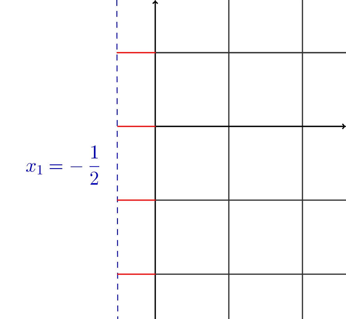
Figure 1: A portion of $\mathcal{H}^{\prime}$ with in red the conductances with value $2$.

Let us begin by adding to $\mathcal{H}$ all the bonds $\{z,z-\nicefrac{{1}}{{2}}\,\mathbf{e}_{(1)}\}$ for all $z\in\{0\}\times\operatorname{\mathbb{Z}}^{d-1}$. Call this new graph $\mathcal{H}^{\prime}$. Let us put for each edge a conductance

$$c_{\mathcal{H}^{\prime}}(x,\,y):=\begin{cases}2&\left\|x-y\right\|=\nicefrac{{1}}{{2}}\\ 1&\mathrm{otherwise}\end{cases}.$$

(see Figure 1 for a two-dimensional example). It is easy to see that $G_{\mathcal{H}^{\prime}}(x,y)=G_{\mathcal{H}}(x,y)$ for all $x,y\in H$ as there is no current flowing through the new bonds and the old ones are unchanged. Also denote by $(L_{n})_{n\geq 0}$ the random walk on $\mathcal{H}^{\prime}$ with transition probabilities given by $p_{xy}:=c_{\mathcal{H}^{\prime}}(x,y)/\pi_{\mathcal{H}^{\prime}}(x)$.

Consider further the graph obtained from $\operatorname{\mathbb{Z}}^{d}$ by splitting the conductance on the bond $\{z-\mathbf{e}_{(1)},z\}$ with $z\in\{0\}\times\operatorname{\mathbb{Z}}^{d-1}$ into two conductances in series on the bonds $\{z-\mathbf{e}_{(1)},z-\nicefrac{{1}}{{2}}\,\mathbf{e}_{(1)}\}$ and $\{z-\nicefrac{{1}}{{2}}\,\mathbf{e}_{(1)},z\}$. More precisely on this new graph, which we call $\mathcal{Q}$, put the following conductances:

$$c_{\mathcal{Q}}(x,\,y):=\begin{cases}2&\left\|x-y\right\|=\nicefrac{{1}}{{2}}\\ 1&\mathrm{otherwise}\end{cases},\quad x,\,y\in\operatorname{\mathbb{Z}}^{d}\cup\left(\{-\nicefrac{{1}}{{2}}\}\times\operatorname{\mathbb{Z}}^{d-1}\right).$$

By Ohm’s law of conductances in series, this ensures that the new graph obtained is equivalent to $\operatorname{\mathbb{Z}}^{d}$. More precisely $g(x,y)=G_{\mathcal{Q}}(x,y)$ for all $x,y\in\operatorname{\mathbb{Z}}^{d}$.

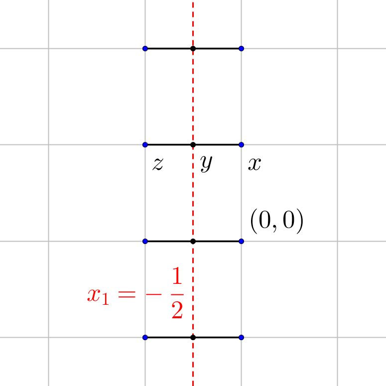
Figure 2: A portion of $\mathcal{Q}.$ Starting from $\operatorname{\mathbb{Z}}^{d}$ (light gray lines), we split the conductance $\{x,z\}$ which has value one in the two conductances $\{x,\,y\}$ and $\{y,\,z\}$ with value two.

Consider the simple random walk $W=(W_{n})_{n\geq 0}$ on $\mathcal{Q}$ with transition probabilities given by $q_{xy}:=c_{\mathcal{Q}}(x,\,y)/\pi_{\mathcal{Q}}(x)$ and started in $H$. Write $W_{n}=\left(U_{n},\,V_{n}\right)$ with $U_{n}$ being the projection of $W_{n}$ on the first coordinate direction and $V_{n}$ the projection of $W_{n}$ on the remaining $d-1$ components. Finally, consider $W^{\prime}=(W^{\prime}_{n})_{n\geq 0}$ which is the reflection of $W$ with respect to the hyperplane $\left\{x\in\operatorname{\mathbb{R}}^{d}:\,x_{1}=-\nicefrac{{1}}{{2}}\right\}$. In other words, $W^{\prime}_{0}=W_{0}$ and $W^{\prime}_{n}=\left(-U_{n}-1,\,V_{n}\right)\mathbbm{1}_{\left\{U_{n}\leq-\nicefrac{{1}}{{2}}\right\}}+(U_{n},\,V_{n})\mathbbm{1}_{\left\{U_{n}>-\nicefrac{{1}}{{2}}\right\}}$.

As we have already mentioned, by electric network reduction (Lyons and Peres, 2016, Section 2.3), we are able to say that $G_{\mathcal{Q}}(x,\,y)=g(x,\,y)$ for all $x,\,y$ and $G_{\mathcal{H}}(x,\,y)=G_{\mathcal{H}^{\prime}}(x,\,y)$ for all $x,y\in H$. Moreover by construction $\pi_{\mathcal{H}^{\prime}}\equiv\pi_{\mathcal{Q}}$ on $H$ and by checking the first step transition probabilities it is easy to notice that $W^{\prime}\stackrel{{\scriptstyle d}}{{=}}\stackrel{{\scriptstyle}}{{L}}$. Therefore, for all $x,\,y\in H$ it holds that

$$G_{\mathcal{H}}(x,\,y) =G_{\mathcal{H}^{\prime}}(x,\,y)=\frac{1}{\pi_{\mathcal{H}^{\prime}}(y)}\mathbb{E}_{x}\left[\sum_{n\geq 0}\mathbbm{1}_{\left\{L_{n}=y\right\}}\right]=\frac{1}{\pi_{\mathcal{Q}}(y)}\mathbb{E}_{x}\left[\sum_{n\geq 0}\mathbbm{1}_{\left\{W_{n}^{\prime}=y\right\}}\right]$$

$$=\frac{1}{\pi_{\mathcal{Q}}(y)}\mathbb{E}_{x}\left[\sum_{n\geq 0}\mathbbm{1}_{\left\{W_{n}=y\right\}}\right]+\frac{1}{\pi_{\mathcal{Q}}(y)}\mathbb{E}_{x}\left[\sum_{n\geq 0}\mathbbm{1}_{\left\{W_{n}=\overline{y}-\mathbf{e}_{(1)}\right\}}\right]$$

$$=G_{\mathcal{Q}}\left(x,\,y\right)+G_{\mathcal{Q}}\left(x,\,\overline{y}-\mathbf{e}_{(1)}\right)$$

where the second equality uses that $W^{\prime}\stackrel{{\scriptstyle d}}{{=}}L.$ The conclusion follows immediately after using that $G_{\mathcal{Q}}(x,\,y)=g(x,\,y)$ for all $x,\,y\in\operatorname{\mathbb{Z}}^{d}$. ∎

Remark 2.

Let $N\in\operatorname{\mathbb{N}}$ and consider the set $C_{N}:=([0,N]\times[-N,N]^{d-1})\cap H$. Let

$$G_{C_{N}}(x,y):=\frac{1}{\pi_{\mathcal{H}}(y)}\mathbb{E}_{x}\left[\sum_{m=0}^{\tau_{C_{N}}}\mathbbm{1}_{\left\{S_{m}=y\right\}}\right],\quad x,\,y\in H,$$

where $\tau_{C_{N}}:=\inf\{m\geq 0:\,S_{m}\notin C_{N}\}.$ In fact we are looking at the Green’s function of a random walk on $H$ which is killed when leaving $C_{N}$. Then by the arguments of Proposition 1 one can guess that

$$G_{C_{N}}(x,y):=g_{K_{N}}(x,\,y)+g_{K_{N}}(x,\,\overline{y}-\mathbf{e}_{(1)})$$ (3.2)

where $K_{N}:=([-N-1,N]\times[-N,N]^{d-1})\cap\operatorname{\mathbb{Z}}^{d}=C_{N}\cup(\overline{C_{N}}-\mathbf{e}_{(1)})$ and $g_{K_{N}}$ is the Green’s function of the simple random walk on $\operatorname{\mathbb{Z}}^{d}$ which is killed when leaving $K_{N}$. Having this guess it is straightforward to verify that this is the right choice since $G_{C_{N}}(\cdot,\,y)$, $y\in H$, is the unique solution to

$$\begin{cases}\sum_{z\sim x,\,z\in H}c_{\mathcal{H}}(z,x)(G_{C_{N}}(z,\,y)-G_{C_{N}}(x,\,y))=-\delta_{x}(z),&x\in C_{N},\\ G_{C_{N}}(x,\,y)=0,&x\notin C_{N}\end{cases}$$

(Lawler and Limic, 2010, Proposition 6.2.2). Notice finally that sending $N\to+\infty$ we get back (3.1) as $g_{K_{N}}(\cdot,\,\cdot)\to g(\cdot,\cdot)$. This approach offers a concise alternative to prove Proposition 1, but is of course based on the “educated guess” (3.2).

Remark 3.

Another natural case which is worth comparing with (3.1) is the Green’s function of the process $(S_{n})_{n\geq 0}=(|S^{(1)}_{n}|,\,S^{(2)}_{n},\dots,\,S^{(d)}_{n})_{n\geq 0}$, where $(S^{(1)}_{n},\,S^{(2)}_{n},\dots,\,S^{(d)}_{n})_{n\geq 0}$ is the simple random walk on $\operatorname{\mathbb{Z}}^{d}$. It is easy to see that $S_{n}$ has the same law of a random walk on $H$ with conductances $c(x,y)$ equal to $\nicefrac{{1}}{{2}}$ if $x_{1}=y_{1}=0$ and equal to one otherwise. Its Green’s function equals

$$g(x,y)+g(x,\overline{y}),\quad x,y\in H.$$

Remark 4.

The Green’s function $G_{\mathcal{H}}$ is not translation invariant and the maximum of $G_{\mathcal{H}}(x,x)$ is on the hyperplane $\{x\in\operatorname{\mathbb{Z}}^{d}:\,x_{1}=0\}$. More precisely it follows from (3.1) that

$$g(0,\,0)=\inf_{x\in H}G_{\mathcal{H}}(x,\,x)<\sup_{x\in H}G_{\mathcal{H}}(x,\,x)=G_{\mathcal{H}}(0,\,0),$$ (3.3)

and that $\lim_{x_{1}\to+\infty}G_{\mathcal{H}}(x,x)=g(0,0)$. Notice that even though we could have proven that $\sup_{x\in H}G_{\mathcal{H}}(x,\,x)=G_{\mathcal{H}}(0,\,0)$ with Rayleigh’s monotonicity law, we could not employ such a technique to obtain the strict inequality (3.3).

4 Green’s function for the strip

The same idea of folding $\operatorname{\mathbb{Z}}^{d}$ on itself allows us to obtain a closed formula for the strip $\mathcal{S}_{L}:=[0,\,L-1]\times\operatorname{\mathbb{Z}}^{d-1}$ for $L\in\{2,\,3,\,\ldots\}$, $d\geq 4$ and nearest-neighbour bonds. The conductances are set to be $c_{\mathcal{S}_{L}}\equiv 1$ for all the bonds.

Proposition 5.

With the above notation one has

$$G_{\mathcal{S}_{L}}(x,\,y)=\sum_{k=-\infty}^{+\infty}\left[g(x,\,(kL+L-1)\mathbf{e}_{(1)}+\overline{y})\mathbbm{1}_{\left\{k\in 2\operatorname{\mathbb{N}}+1\right\}}+g(x,\,kL\mathbf{e}_{(1)}+y)\mathbbm{1}_{\left\{k\in 2\operatorname{\mathbb{N}}\right\}}\right].$$ (4.1)

Proof.

The idea is to apply a so-called "mountain-and-valley" fold to $\operatorname{\mathbb{Z}}^{d}$. We are splitting each of the conductances connecting the points in $L\operatorname{\mathbb{Z}}\times\operatorname{\mathbb{Z}}^{d-1}$ and $L\operatorname{\mathbb{Z}}\times\operatorname{\mathbb{Z}}^{d-1}-\mathbf{e}_{(1)}$, which have value one, into two conductances in series with value two, then we fold $\operatorname{\mathbb{Z}}^{d}$ along the lines $\{x_{1}=kL-\nicefrac{{1}}{{2}}\}$, $k\in\operatorname{\mathbb{Z}}$, as described in Figure 3. This operation will translate a point $A_{0}\in\mathcal{S}_{L}$ into a family of points $\left\{A_{k}\right\}_{k\in\operatorname{\mathbb{Z}}}$, where

$$A_{k}:=\begin{cases}(kL+L-1)\mathbf{e}_{(1)}+\overline{A_{0}}&k\in 2\operatorname{\mathbb{N}}+1\\ kL\mathbf{e}_{(1)}+A_{0}&k\in 2\operatorname{\mathbb{N}}\end{cases}.$$

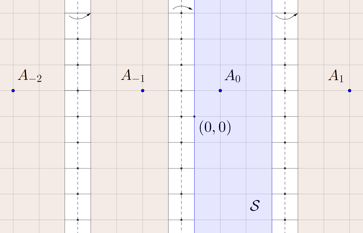
Figure 3: Following traditional origami notation, we are folding the strip and its translates in a mountain (dot dashed) and valley (dashed) fashion. The points $A_{-2},\,A_{-1},\,A_{1}$ are (a few of) the translates of $A_{0}$.

By comparing the random walk on the strip and the projection of the simple random walk onto the strip under the above mentioned folding, one gets (4.1). ∎

Remark 6 (Transience on the strip).

This makes one understand that the Green’s function is constant along hyperplanes of the form $\{x\in\operatorname{\mathbb{Z}}^{d}:\,x_{1}=a\}$, $a=0,\,\ldots,\,L-1$. Note also that our formula combined with the estimate for the transient simple random walk (cf. Lawler and Limic (2010, Theorem 4.3.1))

$$\max\left\{1,\,c_{\ell}\left\|x-y\right\|^{2-d}\right\}\leq g(x,\,y)\leq\max\left\{1,\,c_{r}\left\|x-y\right\|^{2-d}\right\},\quad c_{\ell,}\,c_{r}>0,\;x,\,y\in\operatorname{\mathbb{Z}}^{d}$$ (4.2)

implies that the Green’s function is finite on the diagonal in $d\geq 4$, that is, the random walk is transient on $\mathcal{S}_{L}$.

5 Green’s function on the orthant

Let $\mathcal{O}$ be the subgraph of the $d$-dimensional lattice with vertex set

$$O:=\left\{x\in\operatorname{\mathbb{Z}}^{d}:\,\forall\,i=1,\dots,d:\,x_{i}\geq 0\right\}=\operatorname{\mathbb{N}}_{0}^{d}$$

and nearest-neighbor bonds. This graph is also known with the name of discrete orthant (called “octant” in $d=3$). We set the bonds of $\mathcal{O}$ to have $c_{\mathcal{O}}\equiv 1$.

For $d\geq 3$, the Green’s function of a random walk $(S_{n})_{n\geq 0}$ on $\mathcal{O}$ is given by

$$G_{\mathcal{O}}(x,\,y):=\frac{1}{\pi_{\mathcal{O}}(y)}\mathbb{E}_{x}\left[\sum_{n\geq 0}\mathbbm{1}_{\left\{S_{n}=y\right\}}\right],\quad x,y\in\mathcal{O},$$

where $\pi_{\mathcal{O}}(x):=\sum_{y\sim x}c_{\mathcal{O}}(x,y)$ as usual.

We wish to prove a closed formula for the Green’s function not only for the orthant, but also for more general subgraphs of the lattice in which $m$ components are non-negative. We denote by $\mathcal{U}_{m}$ the graph with vertex set $\operatorname{\mathbb{N}}_{0}^{m}\times\operatorname{\mathbb{Z}}^{d-m}$ and with nearest-neighbor unitary conductances. We call their Green’s function $G_{m}$ in place of $G_{\mathcal{U}_{m}}$ to ease the notation. Also notice that $G_{0}(\cdot,\,\cdot)\equiv g(\cdot,\,\cdot)$ and $G_{d}(\cdot,\,\cdot)\equiv G_{\mathcal{O}}(\cdot,\,\cdot)$.

Proposition 7 (Green’s function on the orthant).

For all $x,\,y\in\mathcal{U}_{m}$

$$G_{m}(x,\,y)=\sum_{v\in\left\{0,\,1\right\}^{m}\times\left\{0\right\}^{d-m}}g\left(x,\,\left((-1)^{v_{i}}\left(y_{i}+\nicefrac{{1}}{{2}}\right)-\nicefrac{{1}}{{2}}\right)_{i=1}^{d}\right).$$ (5.1)

In particular, for all $x,\,y\in\mathcal{\mathcal{O}},$

$$G_{\mathcal{O}}(x,\,y)=\sum_{v\in\left\{0,\,1\right\}^{d}}g\left(x,\,\left((-1)^{v_{i}}\left(y_{i}+\nicefrac{{1}}{{2}}\right)-\nicefrac{{1}}{{2}}\right)_{i=1}^{d}\right).$$ (5.2)

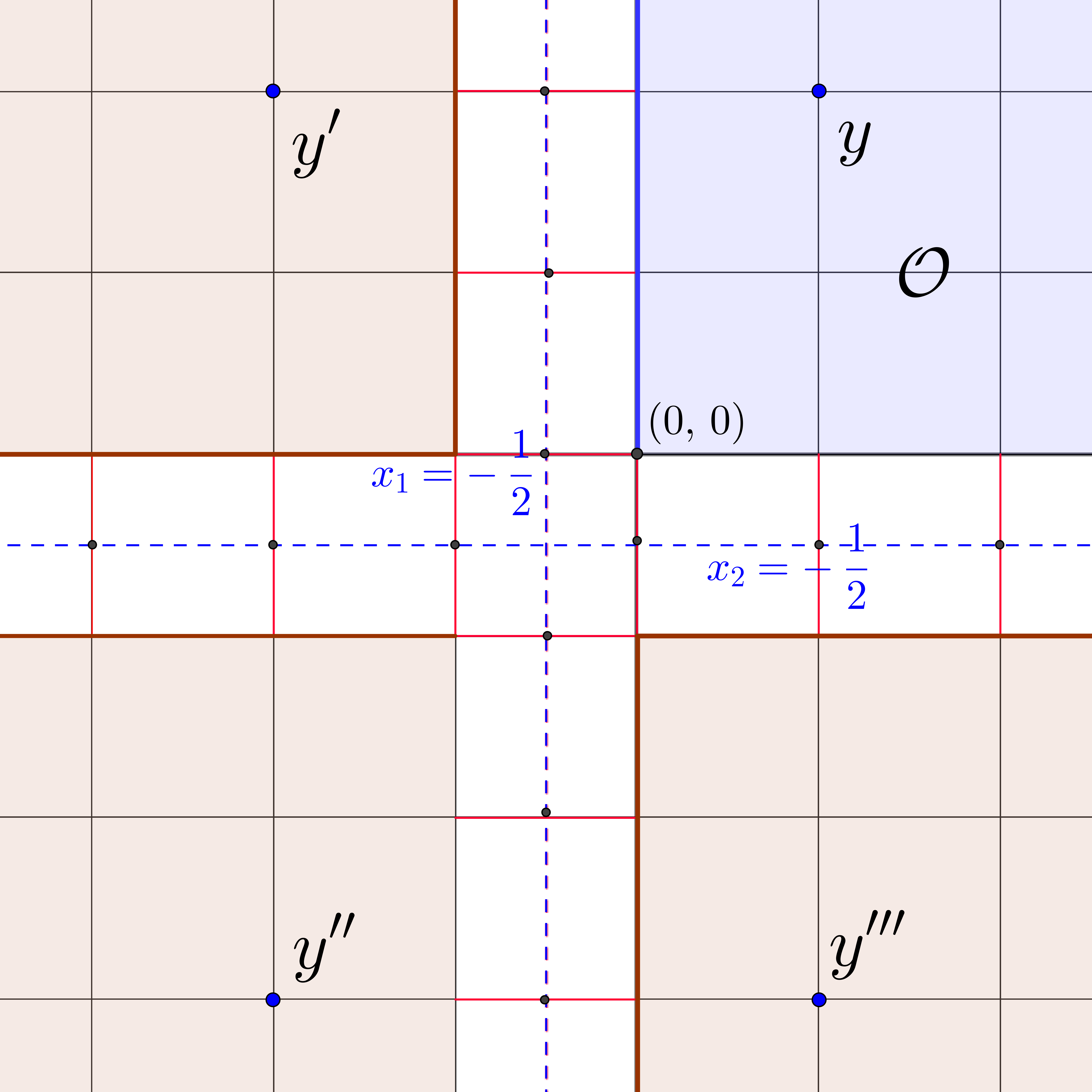
Figure 4: For $y\in\mathcal{O}$, $\left\{\left((-1)^{v_{i}}\left(y_{i}+\nicefrac{{1}}{{2}}\right)-\nicefrac{{1}}{{2}}\right)_{i=1}^{2}:\,v\in\left\{0,\,1\right\}^{2}\right\}=\{y,\,y^{\prime},\,y^{\prime\prime},\,y^{\prime\prime\prime}\}$, in this two-dimensional example.

Proof.

Before we begin, we want to stress that the apparently complicated formulas (5.1) and (5.2) are nothing but a sum over all the reflections of the point $y$ about $m$ axes of the form $\left\{x\in\operatorname{\mathbb{R}}^{d}:\,x_{j}=-\nicefrac{{1}}{{2}}\right\}$ for some $1\leq j\leq d$. Figure 4 clarifies this in the case $m=d$.

The proof is similar to that of Proposition 1 so we will only sketch it here. The notation we adopt is also similar to stress we are essentially going over the same argumentation. Since the orthant is a special case of intersections of $d$ half spaces, we will work directly for a subspace $\mathcal{U}_{m}$ and $m\geq 1$, being $\mathcal{U}_{0}=\operatorname{\mathbb{Z}}^{d}$ trivial.

To $\mathcal{U}_{m}$, we add all the bonds of length $\nicefrac{{1}}{{2}}$ that connect the “face” $\mathcal{F}_{j}:=\left\{x\in\mathcal{U}_{m}:\,x_{j}=0\right\}$ to the shifted “face” $\mathcal{F}_{j}-\nicefrac{{1}}{{2}}\mathbf{e}_{(j)}$ for all $1\leq j\leq m$ and we put on each newly added edge a conductance equal to $2$. Call this new graph $\mathcal{U}_{m}^{\prime}$ and its Green’s function $G^{\prime}_{m}$. Clearly $G^{\prime}_{m}(x,y)=G_{m}(x,y)$ for all $x,y\in\mathcal{U}_{m}$. Denote by $L$ be the random walk on $\mathcal{U}_{m}^{\prime}$ driven by such conductances.

At this point we modify the discrete lattice in a similar way as in Proposition 1. Essentially for all $1\leq j\leq m$ we replace each conductance which connects the hyperplanes $\mathcal{I}_{j}:=\{x\in\operatorname{\mathbb{Z}}^{d}\,:\,x_{j}=0\}$ and $\mathcal{I}_{j}-\mathbf{e}_{(j)}$ by two conductances in series and value two (these are the red bonds in Figure 4). These new conductances have length $\nicefrac{{1}}{{2}}$ and connect $\mathcal{I}_{j}-\nicefrac{{1}}{{2}}\mathbf{e}_{(j)}$ to either $\mathcal{I}_{j}$ or $\mathcal{I}_{j}-\mathbf{e}_{(j)}$ for some $1\leq j\leq m$. Call this new graph $\mathcal{Q}$.

Let $X=(X_{n})_{n\geq 0}=(X^{(1)}_{n},\,\ldots,\,X_{n}^{(d)})_{n\geq 0}$ be the random walk on $\mathcal{Q}$ starting in $\mathcal{U}_{m}$ and $G_{\mathcal{Q}}(\cdot,\,\cdot)$ its Green’s function. Let $Y$ be the reflection of $X$ on the hyperplanes given by $\left\{x\in\operatorname{\mathbb{R}}^{d}:\,x_{j}=-\nicefrac{{1}}{{2}}\,\mathbf{e}_{(j)}\right\}$, $1\leq j\leq m$, that is, $Y_{0}=X_{0}$ and $Y_{n}=(Y_{n}^{(1)},\,\ldots,\,Y_{n}^{(d)})$ with

$$Y_{n}^{(k)}:=\begin{cases}(-X_{n}^{(k)}-1)\mathbbm{1}_{\left\{X^{(k)}_{n}\leq-\nicefrac{{1}}{{2}}\right\}}+X_{n}^{(k)}\,\mathbbm{1}_{\left\{X_{n}^{(k)}>-\nicefrac{{1}}{{2}}\right\}}&1\leq k\leq m,\\ X_{n}^{(k)}&\mbox{otherwise}\end{cases}.$$

We can now use the fact that $G_{m}\equiv G^{\prime}_{m}$ on $\mathcal{U}_{m}\times\mathcal{U}_{m}$, that $G_{\mathcal{Q}}\equiv g$ on $\operatorname{\mathbb{Z}}^{d}\times\operatorname{\mathbb{Z}}^{d}$ and the equivalence of the laws of the random walks $L$ and $Y$ to show that for all $x,y\in\mathcal{U}_{m}$

$$G_{m}(x,\,y) =\sum_{v\in\left\{0,\,1\right\}^{m}\times\left\{0\right\}^{d-m}}g\left(x,\,\left((-1)^{v_{i}}\left(y_{i}+\nicefrac{{1}}{{2}}\right)-\nicefrac{{1}}{{2}}\right)_{i=1}^{d}\right).$$ (5.3)

∎

We are interested now in monotonicity properties of Green’s functions. We could not find in the literature a reference to the next Lemma, so we decided to give a short proof for it. Let $x,\,y\in\operatorname{\mathbb{Z}}^{d}$ and define the partial relation $x\succeq y$ if and only if $|x_{i}|\geq|y_{i}|$ for all $1\leq i\leq d$. This is also known as product order.

Lemma 8 (Monotonicity of $g(0,\,\cdot)$ with respect to the product order).

If $x,\,y\in\operatorname{\mathbb{Z}}^{d}$ and $x\succeq y$, then $g(0,\,x)\leq g(0,\,y)$.

Proof.

We have, from Montroll (1956, Eq. (2.10)), that

$$2dg(0,\,x)=\int_{0}^{+\infty}\mathrm{e}^{-t}\prod_{i=1}^{d}I_{x_{i}}\left(\frac{t}{d}\right)\operatorname{d}t.$$

For $j,\,j^{\prime}\in\operatorname{\mathbb{N}}_{0},$ one has $I_{j}(t)\geq I_{j^{\prime}}(t)$ for all $t\in[0,\,+\infty)$ if $j^{\prime}\geq j$ . Considering also that $I_{-m}=I_{m}$ for $m\in\operatorname{\mathbb{Z}}$ (Abramowitz and Stegun, 1964, Eq. 9.6.6), the product order yields the desired conclusion. ∎

Corollary 9.

$G_{m}(x,\,\cdot)$ is monotone decreasing with respect to the product order for all $x\in\mathcal{U}_{m}$.

Proof.

The result follows combining Proposition 7 with Lemma 8. ∎

Remark 10.

From (5.3) and Lemma 8 above one obtains the location of the maximum of the Green’s function:

$$\sup_{x\in\mathcal{U}_{m}}G_{m}(x,\,x)=G_{m}(0,\,0),\quad 0\leq m\leq d.$$ (5.4)

Another consequence of (5.3) is the following chain of strict inequalities:

$$g(x,\,y)<G_{1}(x,\,y)<\ldots<G_{d}(x,\,y),\quad x,\,y\in\mathcal{O}.$$

More precisely $G_{j}(x,\,y)<G_{j+1}(x,\,y)$ for all $x,y\in\mathcal{U}_{j+1}$ and $0\leq j\leq d-1$.

5.1 A useful formula at the origin

An interesting consequence of our analysis is that we can explicitly calculate (5.3) in the case $x=y=0.$ Namely we show

Lemma 11.

Let $I_{k}(\cdot)$ be the modified Bessel function of the first kind of order $k\in\operatorname{\mathbb{N}}_{0}$. For all $0\leq m\leq d$,

$$G_{m}(0,\,0)=\frac{1}{2d}\int_{0}^{+\infty}\mathrm{e}^{-x}\left(I_{1}\left(\frac{x}{d}\right)+I_{0}\left(\frac{x}{d}\right)\right)^{m}I_{0}\left(\frac{x}{d}\right)^{d-m}\operatorname{d}x.$$ (5.5)

Proof.

Let $\gamma_{j}:=\sum_{k=1}^{j}\mathbf{e}_{(k)}$ for $1\leq j\leq d.$ The formula (5.1) is telling us that, to compute $G_{m}(0,0)$ we have to choose, for each $j\in\{0,...,m\}$, $j$ hyperplanes out of $m$ about which to reflect the point $0$, and then compute the sum of terms of the form $g(0,z)$, where $z$ is one reflection of the origin about these hyperplanes. However, the value of $g(0,z)$ is independent of the $j$ hyperplanes chosen, due to the fact that $g(x,\,y)$ depends only on $\|x-y\|$. This yields

$$G_{m}(0,\,0)=\sum_{j=0}^{m}\binom{m}{j}g\left(0,\,\gamma_{j}\right).$$

As a consequence of Montroll (1956, Eq. (2.11b)) we obtain

$$g\left(0,\,\gamma_{j}\right)=\frac{1}{2d}\int_{0}^{+\infty}\mathrm{e}^{-x}I_{1}\left(\frac{x}{d}\right)^{j}I_{0}\left(\frac{x}{d}\right)^{m-j}I_{0}\left(\frac{x}{d}\right)^{d-m}\operatorname{d}x,\quad j=0,\,\ldots,\,m$$

whence (5.5). ∎

One can use the above formula as a starting point to show asymptotic expansions of $G_{\mathcal{O}}$ for large values of $d$. Furthermore, it appears to be useful to get statements pointwise in the dimension. The corollary below provides a simple example.

Corollary 12.

$2dG_{\mathcal{O}}(0,\,0)$ is decreasing in $d$ for all $d\geq 3$.

Proof.

This is an immediate consequence of Lemma 11. Indeed for $d^{\prime}\geq d$, Abramowitz and Stegun (1964, Eq. 9.6.19) gives that

$$\left(I_{0}\left(\frac{x}{d}\right)+I_{1}\left(\frac{x}{d}\right)\right)^{d}= \left(\int_{0}^{\pi}\mathrm{e}^{\frac{x}{d}\cos\vartheta}\frac{\left(\cos\vartheta+1\right)}{\pi}\operatorname{d}\vartheta\right)^{d}$$

$$\geq\left(\int_{0}^{\pi}\mathrm{e}^{\frac{x}{d^{\prime}}\cos\vartheta}\frac{\left(\cos\vartheta+1\right)}{\pi}\operatorname{d}\vartheta\right)^{d^{\prime}}=\left(I_{0}\left(\frac{x}{d^{\prime}}\right)+I_{1}\left(\frac{x}{d^{\prime}}\right)\right)^{d^{\prime}}$$

where the second line follows from Jensen’s inequality and the fact that the measure $\pi^{-1}\left(\cos\vartheta+1\right)\operatorname{d}\vartheta$ has mass $1$. Plugging this into (5.5) with $m=d$, we can conclude. ∎

References

- Abramowitz and Stegun [1964] M. Abramowitz and I. A. Stegun. Handbook of mathematical functions with formulas, graphs, and mathematical tables, volume 55 of National Bureau of Standards Applied Mathematics Series. For sale by the Superintendent of Documents, U.S. Government Printing Office, Washington, D.C., 1964.
- Bostan et al. [2014] A. Bostan, M. Bousquet-Mélou, M. Kauers, and S. Melczer. On 3-dimensional lattice walks confined to the positive octant. arXiv preprint arXiv:1409.3669, 2014.
- Bousquet-Mélou and Schaeffer [2002] M. Bousquet-Mélou and G. Schaeffer. Walks on the slit plane. Probability Theory and Related Fields, 124(3):305–344, 2002. ISSN 1432-2064. 10.1007/s004400200205. URL http://dx.doi.org/10.1007/s004400200205.
- Denisov and Wachtel [2015] D. Denisov and V. Wachtel. Random walks in cones. Ann. Probab., 43(3):992–1044, 2015. ISSN 0091-1798. 10.1214/13-AOP867. URL http://dx.doi.org/10.1214/13-AOP867.
- Fayolle et al. [1991] G. Fayolle, I. Ignatyuk, V. A. Malyshev, and M. Menshikov. Random walks in two-dimensional complexes. Queueing Systems, 9(3):269–300, 1991.
- Ganguly and Peres [2015] S. Ganguly and Y. Peres. Convergence of discrete Green functions with Neumann boundary conditions. ArXiv e-prints, Mar. 2015. URL http://arxiv.org/abs/1503.06948.
- Kurkova and Malyshev [1998] I. Kurkova and V. Malyshev. Martin boundary and elliptic curves. Markov Process. Related Fields, 4(2):203–272, 1998.
- Lawler and Limic [2010] G. Lawler and V. Limic. Random walk: a modern introduction. Cambridge University Press, Cambridge, 2010.
- Lyons and Peres [2016] R. Lyons and Y. Peres. Probability on Trees and Networks. Cambridge University Press, 2016. Available at http://pages.iu.edu/~rdlyons/.
- Montroll [1956] E. W. Montroll. Random walks in multidimensional spaces, especially on periodic lattices. Journal of the Society for Industrial and Applied Mathematics, 4(4):241–260, 1956. 10.1137/0104014. URL http://dx.doi.org/10.1137/0104014.
- Raschel [2012] K. Raschel. Counting walks in a quadrant: a unified approach via boundary value problems. Journal of the European Mathematical Society, 14:749–777, 2012.
- Uchiyama [2010] K. Uchiyama. The green functions of two dimensional random walks killed on a line and their higher dimensional analogues. Electron. J. Probab., 15:1161–1189, 2010. 10.1214/EJP.v15-793. URL http://dx.doi.org/10.1214/EJP.v15-793.