Exact probability distribution functions for Parrondo’s games

Abstract

We consider discrete time Brownian ratchet models: Parrondo’s games. Using the Fourier transform, we calculate the exact probability distribution functions for both the capital dependent and history dependent Parrondo’s games. We find that in some cases there are oscillations near the maximum of the probability distribution, and after many rounds there are two limiting distributions, for the odd and even total number of rounds of gambling. We assume that the solution of the aforementioned models can be applied to portfolio optimization.

The Parrondo’s games pa96 -ab10 , related to the Brownian ratchets pr92 -ch14 are interesting phenomena at the intersection of game theory, econophysics and statistical physics, see ab10 for the inter-disiplinary applications. In case of Brownian ratchets the particle moves in a potential, which randomly changes between 2 versions. For each there is a detailed balance condition. On average there is a motion due to the random switches between two potentials. The phenomenon is certainly related to portfolio optimization so11 ,so15 . In the related situation in economics, one is using the “volatility pumping” strategy in portfolio optimization, for two asset portfolios, keeping one half of the capital in the first asset, the other half in the second asset with high volatility vo .

J. M. R. Parrondo invented his game following Brownian ratchets for the discrete time case pa96 , to model gambling. An agent uses two biased coins for the gambling, and both strategies are loosing. In some cases a random combination of two loosing games is a winning game. It is interesting that the opposite situation is also possible, a random combination of two winning games can give a loosing game.

Parrondo’s games have been considered either on the one dimensional axis with some periodic potential, or by looking at the time dependent version of the game parameters.

For the first case the state of the system is characterized by the current value of the money $X$, and the choice of the strategy. There is a period $M$ defining the rules, how capital $X$ can move up or down. The rules of the game depend on Mod$(X,M)$, where $M$ is the period of the “potential”. Originally $M=3$ games were considered, then $M=2$ versions of Parrondo’s games were constructed ab02 , as05 . For the history dependent versions of the game the current rules of the game depend on the past, whether there was a growth of capital in the previous rounds or not.

Later many modifications of the games were invented, i.e. different integers $M$ for both games sz14 , the Allison mixture ab14 , where the random mixing of two random sequences creates some autocorrelation ad09a , and two envelope game problems ad10a . Especially intriguing is the recent finding of a Parrondo’s effect-like phenomenon in a Bayesian approach to the modelling of the work of a jury gu16 : the unanimous decision of its members has a low confidence. All the mentioned works consider the situation with random walks, when there are random choices between different strategies during any step, yielding a qualitatively different result than in case of a fixed strategy. In gu16 we have a single choice between the strategies during all the rounds.

In our recent work sa16 we calculated the variance for the history independent case, as the variance of the distributions (volatilities) is important in economics. Now we apply a Fourier transform technique to solve exactly the probability distribution function. The complete distributions are useful to obtain the unknown parameters of the models, describing the data. We apply this method to the random walks on a strip of the chains sa12 , which is the case of the capital dependent Parrondo’s model. We calculate the entire probability distribution for the capital, then solve the same problem for the history dependent game case.

A biased discrete space and time random walk.

As an illustration let us consider the discrete time random walk on the 1-$d$ axis, where the probability of right and left jumps are $p$ and $q$, respectively. We can write the master equation for probability $P(n,t)$ at position $n$ after $t$ steps:

$$P(n,t+1)=$$ (1)

$$pP(n-1,t)+qP(n+1,t)+(1-p-q)P(n,t).$$

We have $P(n,0)=\delta_{n,0}$.

For the motion on the infinite axis we can always write a Fourier transform

$$P(n,t) = \int_{-\pi}^{\pi}dke^{ikn}\bar{P}(k,t),$$

$$\bar{P}(k,t) = \frac{1}{2\pi}\sum_{n}P(n,t)e^{-ikn}$$ (2)

Let the particle start at $n=0$, thus $\bar{P}(k,0)={1}/{2\pi}$.

Eq. (1) transforms into

$$\bar{P}(k,t+1)=\left[pe^{-ik}+qe^{ik}+(1-p-q)\right]\bar{P}(k,t).$$ (3)

We obtain a solution

$$\bar{P}(k,t)=\lambda^{t}(k)\cdot\bar{P}(k,0)$$

$$\lambda(k)=\left[pe^{-ik}+qe^{ik}+(1-p-q)\right]$$ (4)

As $\lambda$ is a linear polynomial in $e^{ik}$ and $e^{-ik}$, $\lambda^{t}$ is a polynomial with powers from $e^{-tik}$ to $e^{tik}$.

We can write the solution as

$$P(n,t)=\int_{-\pi}^{\pi}dke^{tV(ik)+ikn}\bar{P}(k,0),$$

$$V(\kappa):=\ln\left[pe^{-\kappa}+qe^{\kappa}+(1-p-q)\right],$$ (5)

where we defined the function $V(\kappa)$. Using that $\lambda^{t}$ has a finite expansion in powers of $e^{ik}$ we obtain for $\bar{P}(k,0)={1}/{2\pi}$

$$P(n,t)=\frac{1}{2t}\sum_{m=1}^{2t}e^{tV(im\pi/t)+imn\pi/t}$$ (6)

While looking at more involved models, we will use both presentations Eqs. (5),(6).

Note that eqs. (5) and (6) are exact for any $t$ and $n$. By use of the saddle point approximation we derive the large $t$ and $n=xt$ asymptotics. We are allowed to move the integration contour because of the analytic dependence of the integrand on $k$ resulting in ($\kappa=ik$)

$$P(n,t)=\frac{\exp[tu(x)]}{\sqrt{2\pi tV^{\prime\prime}(\kappa)}},$$

$$x=-V^{\prime}(\kappa),u(x)=V(\kappa)+\kappa x$$ (7)

As $u(x)$ is the Legendre transform of $-V(\kappa)$, we also have $V^{\prime\prime}(k)=-1/u^{\prime\prime}(x)$ and hence

$$P(n,t)=\frac{1}{\sqrt{2\pi t}}\exp\left[tu(x)+1/2\log|u^{\prime\prime}(x)|\right],$$

Let us assume an expansion for $V(\kappa)$

$$V(\kappa)=r\kappa+K\kappa^{2}/2$$ (8)

It then follows that

$$<n>=rt,$$

$$<(n-<n>)^{2}>=Kt$$ (9)

The case of several chains

Consider the case of a random walk on the one dimensional axis, using some rules with period $M$.

We divide the entire $x$ axis in intervals of length $M$, $[(n-1)M,nM],n\geq 1$, considering $l=\rm{Mod}(X,M)$. We represent the sets of $p_{X}$ (the discrete probability distribution of the capital value) as $P_{l}(n,t),0\leq l<M$. An integer $t$ represents the time.

One can write the following master equation mo00

$$P_{l}(n,t+1) = A_{l_{-}}P_{l_{-}}(\hat{n},t)+B_{l_{+}}P_{l_{+}}(\bar{n},t)$$ (10)

$$+(1-A_{l}-B_{l})P_{l}(n,t)$$

where $l_{-}={\rm Mod}(l-1,M),{l_{+}={\rm Mod}(l+1,M)}$, $\hat{n}=n$ for $l-1\geq 0$ and $\hat{n}=n-1$ for $l-1<0$; $\bar{n}=n$ for $l+1<M$ and $\bar{n}=n+1$ for $l+1>M$. Thus the model is characterized by the parameters $A_{l},B_{l}$, where $A_{l}$ and $B_{l}$ are the probabilities to win and lose for the capital $X$ with $l=\rm{Mod}(X,M)$.

We again consider the Fourier transform

$$P_{l}(n,t)=\int_{-\pi}^{\pi}dke^{ikn}\bar{P}_{l}(k,t)$$ (11)

Then we obtain

$$\bar{P}_{l}(k,t+1) = A_{l_{-}}e^{ik(\hat{n}-n)}\bar{P}_{l_{-}}(k,t)+B_{l_{+}}e^{ik(\bar{n}-n)}v_{l_{+}}$$ (12)

$$+(1-(A_{l}+B_{l}))\bar{P}_{l}(k,t)$$

$$\equiv \sum_{m=0}^{M-1}\hat{Q}_{lm}(ik)\bar{P}_{m}(k,t)$$

Using the eigenvalues and eigenvectors $\lambda_{m}(\kappa),v_{ml}(\kappa)$ ($m=0,...,M-1$), of the matrix $Q(\kappa)$, we find

$$\bar{P}_{l}(n,t)=\int_{-\pi}^{\pi}dke^{ikn}\sum_{m}c_{m}\exp[tV_{m}]v_{ml},$$ (13)

where $V_{m}(\kappa):=\ln(\lambda_{m}(\kappa))$ and $c_{m}(\kappa)$ are factors determined by the initial distribution. While using Eq. (7), we choose as $V(\kappa)$ the eigenvalue function $V_{m}(\kappa)$ yielding the maximal value of $u(x)$. Close to the maximum of the distribution of $u(x)$ there is a single choice, later we see a possibility for different sub-phases in our model, related to the existence of M different eigenvalues. The large deviation (decoding error) probability in optimal coding theory gal is similar to our case and has several sub-phases. To compare our results for the rate with the formulas in ab02 we have to multiply the rate in Eq. (9) with a factor $M$, as one step in $n$ in our approach equals $M$ ordinary steps. We deduced Eqs. (8),(9) for the mean growth of capital, i.e. for the case of the random walk on the strip.

The eigenvalues $\pm 1$

Next we investigate more closely the case $A_{l}+B_{l}=1$ for all $l$ in (12).

Consider first the case of odd $M$: $Q(0)$ has one eigenvalue +1 with left eigenstate $(1,1,1,1...)$, and $Q(\pi i)$ has one eigenvalue -1 with left eigenstate $(1,-1,1,-1...)$ and the two “wavenumbers” $\kappa=0$ and $\kappa=\pi i$ contribute in the Fourier representation to the stationary state.

Let us now consider the matrices $Q(\kappa)$ and $Q(\kappa+\pi i)$ for arbitrary $\kappa$. It is easy to see that the spectra are simply related. Let $(x_{0},x_{1},x_{2},...)^{T}$ be a right eigenvector of $Q(\kappa)$ with eigenvalue $\lambda(\kappa)$, then $(x_{0},-x_{1},x_{2},...)^{T}$ is a right eigenvector of $Q(\kappa+\pi i)$ with eigenvalue $-\lambda(\kappa)$.

Let as assume an expansion like Eq. (8) for the leading $V(\kappa)$ near $\kappa=0$, then

$$V(\pi+\kappa)=\pi i+r\kappa+K\kappa^{2}/2$$ (14)

Let $v^{+}$ and $v^{-}$ the right eigenstates of $Q(0)$ and $Q(\pi i)$ with eigenvalues $+1$ and $-1$. There are constants $\alpha$ and $\beta$ such that

$$P_{l}(n,t)=\frac{\alpha v_{l}^{+}+(-1)^{n+t}\beta v^{-}_{l}}{\sqrt{2Kt\pi}}e^{-\frac{(n-rt)^{2}}{2Kt}}$$ (15)

We see oscillations caused by the rapid sign change of the second term. The coefficients $\alpha$ and $\beta$ are determined by the initial probability distribution. If this has been concentrated in $n=l=0$ then $\alpha=\beta$ (with $v^{+}$ and $v^{-}$ related as pointed out above). In this case $P_{l}(n,t)$ is non-zero (zero) for even (odd) $l+n+t$.

Consider now the case of even $M$. Here, $\hat{Q}(0)$ has one eigenvalue 1 with left eigenstate $(1,1,1,1...)$ and one eigenvalue -1 with left eigenstate $(1,-1,1,-1...)$. Hence, only the “wavenumber” $\kappa=0$ contributes in the Fourier representation to the stationary state, but with two eigenvalues. Let $(x_{0},x_{1},x_{2},...)^{T}$ be a right eigenvector of $Q(\kappa)$ with eigenvalue $\lambda(\kappa)$, then $(x_{0},-x_{1},x_{2},...)^{T}$ is also a right eigenvector of $Q(\kappa)$, but with eigenvalue $-\lambda(\kappa)$. Now we find similar to the case above

$$P_{l}(n,t)=\frac{\alpha v_{l}^{+}+(-1)^{t}\beta v^{-}_{l}}{\sqrt{2Kt\pi}}e^{-\frac{(n-rt)^{2}}{2Kt}}.$$ (16)

Note that the oscillating factor does not depend on $n$. For a probability initially concentrated in $n=l=0$ we find $P_{l}(n,t)$ is non-zero (zero) for even (odd) $l+t$.

The findings in both cases, odd $M$ and even $M$, can however be summarized: $P_{l}(n,t)$ is non-zero (zero) for even (odd) $l+nM+t$.

It is quite interesting to consider the quantity

$$\hat{P}(n,t)=\sum_{l=0}^{M-1}P_{l}(n,t)$$ (17)

It shows non-zero oscillations in dependence on $n$ and $t$ for odd $M$. Such oscillations do not exist for even $M$. The reason for this is easily understood: $(1,-1,1,-1...)$ and $(x_{0},x_{1},x_{2},...)^{T}$ are left and right eigenvector of $Q(0)$ with eigenvalues $-1$ and $+1$. Hence their product must be zero. This product, however, is equal to the term entering $P(n,t)$ with a $(-1)^{t}$ factor.

Two expressions for the capital growth rates Consider capital depending Parrondo’s game with $p_{1},...,p_{M}$ for the winning probabilities for the corresponding Mod$(X,M)$. We have a corresponding Matrix

$$Q(\kappa)=\begin{pmatrix}0&p_{1}&...&p_{M}e^{-\kappa}\\ .&.&.&.\\ .&.&.&.\\ q_{1}e^{\kappa}&p_{1}&...&0\end{pmatrix}$$ (18)

Applying the method of ab02 gives

$$r=\frac{\sum_{i}(p_{i}-q_{i})x_{i}}{\sum_{i}x_{i}}$$ (19)

We prove that Eqs. (8,Exact probability distribution functions for Parrondo’s games) give the same result. Let us denote by $\lambda(\kappa)$ the largest eigenvalue of $Q(\kappa)$ with left and right eigenstates $\langle y(\kappa)|$ and $|x(\kappa)\rangle$. For $\kappa=0$ we have $\lambda(0)=1$ and $\vec{y}=(1,1,...,1)$. The growth rate $r$ is the first derivative of of $\log\lambda(\kappa)$ at $\kappa=0$. As $\lambda(0)=1$ we find $r=\lambda^{\prime}(0)$, hence

$$r=\frac{\partial}{\partial\kappa}\frac{\langle y(\kappa)|Q(\kappa)|x(\kappa)\rangle}{\langle y(\kappa)|x(\kappa)\rangle}=\frac{\langle y(0)|Q^{\prime}(0)|x(0)\rangle}{\langle y(0)|x(0)\rangle}$$ (20)

where the last equality follows from the Hellmann-Feynman theorem. Using the explicit form of the matrix $Q(\kappa)$, $\langle y(0)|=(1,1,...,1)$, and $|x(0)\rangle=(x_{1},x_{2},...,x_{M})^{T}$ we find

$$r=\frac{p_{M}x_{M}-q_{1}x_{1}}{\sum_{i}x_{i}}$$ (21)

Now we prove the equivalence of Eq. (19) and Eq. (21). The eigenvalue equation for the right eigenstate $(x_{1},x_{2},...,x_{M})^{T}$ of Q(0) for eigenvalue 1 is

$$p_{i-1}x_{i-1}+q_{i+1}x_{i+1}=x_{i}$$ (22)

for all $i$. From this we derive

$$p_{i-1}x_{i-1}-q_{i}x_{i}=x_{i}-q_{i+1}x_{i+1}-q_{i}x_{i}=p_{i}x_{i}-q_{i+1}x_{i+1}$$

where the first equality is simply (22) and the second equality is due to $q_{i+1}=1-p_{i+1}$. Hence $p_{i-1}x_{i-1}-q_{i}x_{i}$ is independent of $i$ and the sum over this term for all $i$ is simply $M$ times the first term for $i=1$. The sum over all terms can be written like

$$\sum_{i}(p_{i}-q_{i})x_{i}=M(p_{0}x_{0}-q_{1}x_{1})=M(p_{M}x_{M}-q_{1}x_{1})$$ (23)

where we used cyclic “boundary condition” $x_{0}=x_{M}$. This completes the proof.

The M=3 Parrondo’s games. Let us apply the theory of the previous subsection to the concrete case of $M=3$ Parrondo’s game. We have two games. The first game is a random walk on the 1-d axis with probability $h$ for the right jumps and probability $(1-h)$ for the left jumps. For the second game the jump parameters depend on the capital value. The probability for the right jumps is $r$ for mod$(X,3)\neq 0$ and $s$ for the case mod$(X,3)=0$. We randomly choose the game every round.

We solve the master equation (10) for calculating the probability distribution after $t$ rounds. The results of iterative numerics are given in Figures (1), (2).

We see that after $t=50$ there is an oscillation near the maximum, then as time passes the number of oscillations grows.

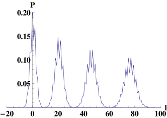
Figure 1: The probability distribution for the capital growth $\hat{P}(n,t)$ (see Eq. (17)) for $t=50,150,200$ for the $M=3$ Parrondo’s model with the $p=0.5-ep,p_{1}=0.75-ep,p_{2}=0.1-ep,ep=0.005$, see Eq. (27). We moved the distributions horizontally for the proper illustration. Our analytical results by Eq.(6) are identical to the results of numerics.

Let us derive this distribution analytically.

We obtain for the matrix $\hat{Q}(\kappa)$

$$\left(\begin{array}[]{ccc}0&(1-p_{1})&p_{2}e^{-\kappa}\\ p_{1}&0&(1-p_{2})\\ (1-p_{1})e^{\kappa}&p_{1}&0\end{array}\right)$$ (27)

For a random choice of the game we have $p_{1}=(h+s)/2,p_{2}=(h+r)/2$. Then Eqs. (12), (13) provide an exact solution.

The $M=3$ game with zero probability for holding the capital at the current value, has peculiar properties: the probability distribution is nonzero for odd differences in the capital after an odd number of time steps, and for even differences after even time steps.

We checked that there are smooth limiting distributions for the even and odd $n$’s, see Fig. 2.

Figure 2: a) $p(x)=\hat{P}(n,t),x=n/t-r,t=1000$ for even $l$ for the $M=3$ Parrondo’s game with the same parameters as for Fig. 1. b) $p(x)=\hat{P}(n,t)$ for odd $l$. The smooth lines are derived according to our asymptotic formulas and Eq. (15), the dashed lines correspond to the numerics.

It is important to find the possibility of transition between different subphases.

Consider the $M=2$ game. For this game we have the right jump probabilities $p_{1},p_{2}$ and left jump probabilities $q_{1},q_{2}$. For a second game on a single axis we have the corresponding probabilities $h,1-h$.

We obtain for the matrix $\hat{Q}(\kappa)$

$$\left(\begin{array}[]{cc}1-(p_{1}+q_{1})&q_{2}+p_{2}e^{-\kappa}\\ p_{1}+q_{1}e^{\kappa}&1-(p_{2}+q_{2})\end{array}\right)$$ (30)

We give the characteristic equation to define the function $V(k)$ in the appendix.

Consider the case of random walks with memory. We denote the up motion as +, down as -. Then the parameters of the motion depend on $\alpha_{1},\alpha_{2}$. We define the current state as $X,\alpha_{1},\alpha_{2}$. Then we get

$$P(X,+,\alpha,t+1) = P(X-1,\alpha,\beta,t)p_{\alpha,\beta}$$

$$P(X,-,\alpha,t+1) = P(X+1,\alpha,\beta,t)(1-p_{\alpha,\beta})$$ (31)

Let us introduce $w(X,t),y(X,t),z(X,t),h(X,t)$ for $(-,-),(-,+),(+,-),(+,+)$ cases, with corresponding probabilities of the right jumps $p_{1},p_{2},p_{3},p_{4}$.

Then we have the master equations

$$w(X,t+1) = w(X+1,t)(1-p_{1})+z(X+1,t)(1-p_{3})$$

$$y(X,t+1) = w(X-1,t)p_{1}+z(X-1,t)p_{3}$$

$$z(X,t+1) = y(X+1,t)(1-p_{2})+h(X+1,t)(1-p_{4})$$

$$h(X,t+1) = y(X-1,t)p_{2}+h(X-1,t)p_{4}$$

Performing a Fourier transformation we get

$$w(X,t)=v_{1}\exp[tu(X/t)],y(X,t)=v_{2}\exp[tu(X/t)]$$

$$z(X,t)=v_{3}\exp[tu(X/t)],h(X,t)=v_{4}\exp[tu(X/t)]$$ (33)

Finally, we obtain a system of equations

$$v_{1}\lambda = v_{1}(1-p_{1})e^{\kappa}+v_{3}(1-p_{3})e^{\kappa}$$

$$v_{2}\lambda = v_{1}p_{1}e^{-\kappa}+v_{3}p_{3}e^{-\kappa}$$

$$v_{3}\lambda = v_{2}(1-p_{2})e^{\kappa}+v_{4}(1-p_{4})e^{\kappa}$$

$$v_{4}\lambda = v_{2}p_{2}e^{-\kappa}+v_{4}p_{4}e^{-\kappa}$$ (34)

In conclusion, we considered the general version of Parrondo’s games. The Parrondo’s games, discovered 2 decades ago, describe a counter-intuitive phenomenon in financial mathematics. Later the model found many inter-disciplinary applications, when a random mixture of two bad strategies gives a good strategy, also conversely too many good witnesses result in low confidence. For most applications it is critical to find the capital growth rate, to find the variance of the distribution. We calculated not only these characteristics of the models, also we found an exact distribution function. The tail of the distribution is interesting for the applications. We calculated also the asymptotics of the distribution for large $t$. The u(x) function satisfies a highly non-linear differential equation, but has an explicit expression as the Legendre transform of an explicitly known ($M=1$) resp. more or less explicitly known function $(M>1)$ of the momentum. For $M>1$ we have to do an eigenvalue analysis. An interesting finding is the existence of oscillations in the probability distribution of the capital after some rounds of gambling and the existence of two limiting distributions. This is a typical situation with the real data of stock fluctuations in financial market, and it is nice that our toy model describes the phenomenon. We see also that different sub-phases are possible while looking the large deviations from the mean values, i.e. the case in optimal coding gal . How realistic is the Parrondo’s phenomenon? As we underlined, it assumes a possibility to use a simple switch (degree of the mixing between several strategies), either strengthening the system or attenuating it. As we discussed in sa05 , the latter situation with the possibility of anti-resonance, is typical for the complex enough living systems.

We thank Bernard Derrida for discussions. DBS thanks MOST 104-2811-M-001-102. grant, as well as Academia Sinica for the support.

References

- (1) J. M. R. Parrondo, How to cheat a bad mathematician, in EEC HC&M Network on Complexity and Chaos (# ERBCHRX-CT940546), ISI, Torino, Italy (1996), Unpublished.
- (2) G. P. Harmer and D. Abbott, Stat. Sci. 14, 206 (1999).
- (3) G. P. Harmer and D. Abbott, Nature 402, 864 (1999).
- (4) J. M. R. Parrondo, G. P. Harmer, D. Abbott, Phys. Rev. Lett., 85, 5226(2000).
- (5) H. Moraal 2000 J. Phys. A: Math. Gen. 33, L203(2000).
- (6) G. P. Harmer, D. Abbott, P. G. Taylor, J. M. R. Parrondo Journal Chaos, 11,705(2001).
- (7) G. P. Harmer and D. Abbott, Fluctuation and Noise Letters 2, R71 (2002).
- (8) D. Abbott Fluctuation and Noise Letters 9, 129(2010).
- (9) A. Ajdari and J. Prost, C. R. Acad. Sci. Paris 315, 1635 (1992).
- (10) R. D. Astumian and M. Bier, Phys. Rev. Lett. 72, 1766 (1994).
- (11) R. D. Astumian, Science, 276,917(1997).
- (12) H. Qian Phys. Rev. Lett. 81, 3063(1998).
- (13) A. Gnoli, A. Petri, F. Dalton,et al Phys. Rev. Lett. 110, 120601 (2013).
- (14) P. Amengual, A. Allison, R. Toral, D. Abbott Proceedings of the Royal Society of London. Series A: 460,2269 (2004).
- (15) Y. Chen and W. Just Phys. Rev. E 90 042102 (2014)
- (16) W.-X. Zhou, G.-H. Mu, W. Chen, D. Sornette,PLoS ONE, 6, e24391(2011).
- (17) Z. Forr , R. Woodard, and D. Sornette, Phys. Rev. E (2015).
- (18) Luenberger, David G., 1997, Investment Science Oxford University Press, New York.
- (19) R. D. Astumian, American journal of physics, 73,178(2005).
- (20) D. Wu and K. Y. Szeto Phys. Rev. E 89, 022142(2014).
- (21) L. J. Gunn, A. Allison and D. Abbott, International Journal of Modern Physics: Conference Series 331460360 (2014).
- (22) D. Abbott, Applications of Nonlinear Dynamics, eds. V. P. Longhini and A. Palacios (Springer-Verlag, Berlin, 2009), p. 307.
- (23) D. Abbott, B.R. Davis, J.M. R. Parrondo, Fluctuation and Noise Letters 9:1 (2010).
- (24) L. J. Gunn, Proc. R. Soc. A 472: 20150748 (2016).
- (25) D.B. Saakian, JSTAT/2016/043213.
- (26) H. Touchette, Phys. Reports, 478,1 (2009).
- (27) V. Galstyan and D. B. Saakian: Phys. Rev. E. 86 (2012) 011125.
- (28) D.B.Saakian, Phys.Rev.E 71, 016126(2005).
- (29) R. G. Gallager, Information Theory and Reliable Communication, (1968), Wiley.