A class of multi-marginal $c$-cyclically monotone sets
with explicit $c$-splitting potentials

Abstract

Multi-marginal optimal transport plans are concentrated on $c$-splitting sets. It is known that, similar to the two-marginal case, $c$-splitting sets are $c$-cyclically monotone. Within a suitable framework, the converse implication was very recently established by Griessler. However, for an arbitrary cost $c$, given a multi-marginal $c$-cyclically monotone set, the question whether there exists an analogous explicit construction to the one from the two-marginal case of $c$-splitting potentials is still open. When the margins are one-dimensional and the cost belongs to a certain class, Carlier proved that the two-marginal projections of a $c$-splitting set are monotone. For arbitrary products of sets equipped with cost functions which are sums of two-marginal costs, we show that the two-marginal monotonicity condition is a sufficient condition which does give rise to an explicit construction of $c$-splitting potentials. Our condition is, in principle, easier to verify than the one of multi-marginal $c$-cyclic monotonicity. Various examples illustrate our results. We show that, in general, our condition is sufficient; however, it is not necessary. On the other hand, we conclude that when the margins are one-dimensional equipped with classical cost functions, our condition is a characterization of $c$-splitting sets and extends classical convex analysis.

2010 Mathematics Subject Classification: Primary 49K30, 49N15; Secondary 26B25, 47H05, 52A01, 91B68.

Keywords: $c$-convex, $c$-monotone, $c$-splitting functions, $c$-splitting set, cyclically monotone, Monge-Kantorovich, multi-marginal, optimal transport.

1 Introduction

In the past decade multi-marginal optimal transport has attracted considerable attention and is now a rapidly growing field of research. Applications can be found in mathematical finance, economics, image processing, tomography, statistics, decoupling of PDEs, mathematical physics and more. Unified and detailed accounts of multi-marginal optimal transport theory, and recent developments and applications, can be found in the surveys [10, 21] and references therein. Naturally, considerable effort is being invested into generalizing the much better understood and established optimal transport theory in the two-marginal case. We focus our attention on an issue of this flavour which underlies the very basic structure of optimal transport. Let $(X_{1},\mu_{1}),\ldots,(X_{N},\mu_{N})$ be Borel probability spaces. We set $X=X_{1}\times\cdots\times X_{N}$ and we denote by $\Pi(X)$ the set of all Borel probability measures $\pi$ on $X$ such that the marginals of $\pi$ are the $\mu_{i}$’s. Let $c:X\to\mathbb{R}$ be a cost function. A cornerstone of multi-marginal optimal transport theory is Kellerer’s [16] generalization of the Kantorovich duality theorem to the multi-marginal case (recent generalizations of Kellerer’s duality theorem are accounted in the surveys mentioned above). Kellerer’s duality theorem asserts that, in a suitable framework,

$$\min_{\pi\in\Pi(X)}\int_{X}c(x)d\pi(x)=\max_{\begin{array}[]{c}u_{i}\in L_{1}({\mu_{i}}),\\ \sum_{1\leq i\leq N}u_{i}\ \leq\ c\end{array}}\ \ \sum_{1\leq i\leq N}\int_{X_{i}}u_{i}(x_{i})d\mu_{i}(x_{i}).$$ (1)

Furthermore, if $\pi$ is a solution of the left-hand side of (1) and $(u_{1},\ldots,u_{N})$ is a solution of the right-hand side of (1), then $\pi$ is concentrated on the subset $\Gamma$ of $X$ where the equality $c=\sum_{1\leq i\leq N}u_{i}$ holds. In recent publications (see [17, 15, 19]) such subsets $\Gamma$ of $X$ are referred to as $c$-splitting sets (see also Definition 2.2 below). It was observed (see, for example, [18, 17]) that $c$-splitting sets are, in fact, $c$-cyclically monotone sets in the multi-marginal sense (see the explicit Definition 2.1 and Fact 2.3 below). Recent studies and applications of multi marginal $c$-cyclic monotonicity and related concepts in the framework of multi-marginal optimal transport include [13, 14, 21, 9, 4]. In the two-marginal case it is well known that a subset $\Gamma$ of $X$ is a $c$-splitting set if and only if $\Gamma$ is $c$-cyclically monotone. Furthermore, given a $c$-cyclically monotone set $\Gamma$, an explicit construction of $c$-splitting potentials $(u_{1},u_{2})$, a generalization of Rockafellar’s explicit construction from classical convex analysis (see Definition 2.5 and Fact 2.6 below) is also well known. In this case $(u_{1},u_{2})$ is a solution of the right hand side of (1). In fact, this construction holds within the most general framework of $c$-convexity theory and applies for general sets $X_{1},\ X_{2}$ and a general coupling (cost) function $c$. Given additional properties of $\Gamma$ and $c$, in the two-marginal case, other explicit techniques, such as integration in $\mathbb{R}^{d}$, can sometimes be applied in order to produce a $c$-splitting solution $(u_{1},u_{2})$. In the multi-marginal case $N\geq 3$, for general sets $X_{1}\ldots,X_{N}$ and a general cost function $c:X\to\mathbb{R}$, given a $c$-cyclically monotone set $\Gamma\subseteq X$, it is an interesting open question whether there exist $c$-splitting potentials $(u_{1},\ldots,u_{N})$ of $\Gamma$. Very recently, within a reasonable framework, existence was established by Griessler [15] using topological arguments. However, even when existence is known, an explicit construction is still not available and there is no multi-marginal counterpart of the construction in Definition 2.5.

In this paper we focus our attention on a fairly general and extensively studied class of cost functions $c$ (see (8) below) which are sums of two-marginal coupling functions. We introduce a class of subsets $\Gamma$ of $X$ by imposing a $c$-cyclical monotonicity condition on their two-marginal projections (see (3) below). In the case where $X_{i}=\mathbb{R}$ for each $i$, for a certain class of cost functions $c$, Carlier [6] established (see also Pass [21]) that the monotonicity of the two-marginal projections of the set $\Gamma\subseteq X$ is a necessary condition on $\Gamma$ in order that it is a $c$-splitting set. For arbitrary sets $X_{i}$ equipped with a cost function from the class of our subject matter, we show that, in fact, this condition is sufficient for $\Gamma$ in order to be a $c$-splitting set. This enables us to employ existing two-marginal solutions in order to explicitly construct solutions to the multi-marginal problem of finding $c$-splitting tuples $(u_{i},\ldots,u_{N})$ for a given set $\Gamma$ satisfying our condition. Another advantage of our approach is that, in principle, it is easier to verify that a given set $\Gamma$ satisfies our condition than verifying that $\Gamma$ satisfies the more general condition of multi-marginal $c$-cyclic monotonicity (see Remark 2.8 below). We then focus our attention on classical cost functions (see Definition 3.1 below). We provide several examples of our construction and show that our condition on a given set $\Gamma$ is sufficient, however, it is not necessary in order to ensure that $\Gamma$ is $c$-cyclically monotone. More explicitly, we present a $c$-cyclically monotone set $\Gamma$ with an explicit $c$-splitting tuple $(u_{1},\ldots,u_{N})$ of $\Gamma$ which does not satisfy our condition. On the other hand, when we focus our attention further on classical cost functions with one-dimensional margins, by combining our discussion with the known results regarding the necessity of the two-marginal condition, we conclude a characterization of $c$-splitting sets. Thus, in this case, given any $c$-cyclically monotone set, using our technique, one can construct an explicit $c$-splitting tuple.

The rest of the paper is organized as follows: In the reminder of this section we collect necessary notations and conventions. In Section 2, we discuss multi-marginal $c$-cyclically monotonicity for products of arbitrary sets and present our more particular class of $c$-cyclically monotone sets along with an explicit construction of $c$-splitting tuples. In Section 3 we review classical cost functions and present examples of our construction and of $c$-cyclically monotone sets which do not fit within our framework. Finally, in Section 4 we focus on classical cost functions with one-dimensional marginals and show that in this case our class of sets is precisely the class of $c$-cyclically monotone sets and generalize other characterizations from the two-marginal case.

Let $Y$ and $Z$ be sets. Given a function $f:Y\to\,\left]-\infty,+\infty\right]$, we say that $f$ is proper if $f\not\equiv+\infty$. Given a multivalued mapping $M:Y\rightrightarrows Z$, we denote by $\operatorname{gra}(M)$ the graph of $M$, that is, $\operatorname{gra}(M)=\{(y,z)\in Y\times Z\ |\ z\in M(y)\}$. We will denote the identity mapping on a given set by $\operatorname{Id}$. Let $S$ be a subset of $Y$. The indicator function of $S$ is the function $\iota_{S}:Y\to\,\left]-\infty,+\infty\right]$ defined by

$$\iota_{S}(y)=\begin{cases}0,&\text{if $y\in S$;}\\ +\infty,&\text{if $y\notin S$.}\end{cases}$$

Throughout our discussion, $N\geq 2$ is a natural number and $I=\{1,\ldots,N\}$ is an index set. Unless mentioned otherwise, $X_{1},\ldots,X_{N}$ are arbitrary nonempty sets, $X=X_{1}\times\cdots\times X_{N}$ and $c:X\to\mathbb{R}$ is a function. Set $P_{i}\colon X\to X_{i}\colon(x_{1},\ldots,x_{N})\mapsto x_{i}$ and $P_{i,j}\colon X\to X_{i}\times X_{j}\colon(x_{1},\ldots,x_{N})\mapsto(x_{i},x_{j})$ for $i$ and $j$ in $\{1,\ldots,N\}$ and when $i<j$. Given a subset $\Gamma$ of $X$, we set

$$\Gamma_{i}=P_{i}(\Gamma)$$ (2)

and

$$\Gamma_{i,j}=P_{i,j}(\Gamma).$$ (3)

Suppose momentarily that $N=2$. Given a function $f_{1}:X_{1}\to[-\infty,+\infty]$, its $c$-conjugate function $f_{1}^{c}:X_{2}\to[-\infty,+\infty]$ is defined by

$$f_{1}^{c}(x_{2})=\sup_{x_{1}\in X_{1}}\ \big{(}c(x_{1},x_{2})-f_{1}(x_{1})\big{)},\ \ \ x_{2}\in X_{2}.$$

Similarly, the $c$-conjugate of $f_{2}:X_{2}\to[-\infty,+\infty]$ is the function $f_{2}^{c}:X_{1}\to[-\infty,+\infty]$ defined by

$$f_{2}^{c}(x_{1})=\sup_{x_{2}\in X_{2}}\ \big{(}c(x_{1},x_{2})-f_{2}(x_{2})\big{)},\ \ \ x_{1}\in X_{1}.$$

Clearly, for any function $f:X_{1}\to\,\left]-\infty,+\infty\right]$,

$$c(x_{1},x_{2})\leq f(x_{1})+f^{c}(x_{2})\ \ \ \mathrm{for\ all}\ (x_{1},x_{2})\in X.$$ (4)

When $N\geq 3$, $c$-conjugation is also widely used in the multi-marginal optimal transport literature mentioned above; however, this will not be a part of our discussion. The case of equality in (4) is captured in the definition of the $c$-subdifferential: Let $f:X_{1}\to\,\left]-\infty,+\infty\right]$ be a proper function. The $c$-subdifferential of $f$ is the mapping $\partial_{c}f:X_{1}\rightrightarrows X_{2}$ defined by

$$\partial_{c}f(x_{1})=\ \big{\{}x_{2}\in X_{2}\ \big{|}\ f(x_{1})+c(x^{\prime}_{1},x_{2})\leq f(x^{\prime}_{1})+c(x_{1},x_{2})\ \ \forall x^{\prime}_{1}\in X_{1}\big{\}}$$

$$=\ \big{\{}x_{2}\in X_{2}\ \big{|}\ f(x_{1})+f^{c}(x_{2})=c(x_{1},x_{2})\big{\}}.$$ (5)

When $M:X_{1}\rightrightarrows X_{2}$ and $\operatorname{gra}(M)\subseteq\operatorname{gra}(\partial_{c}f)$, we say that $f$ is a $c$-antiderivative of $M$. In classical settings, say, when $X_{1}=X_{2}=H$ is a real Hilbert space and $c=\langle{{\cdot},{\cdot}}\rangle$ is the inner product on $X$, $f^{c}=f^{*}$ is the classical Fenchel conjugate function of $f$ and $\partial_{c}f=\partial f$ is the classical subdifferential of $f$. Let $A:H\to H$ be linear and bounded. The quadratic form of $A$ is the function $q_{A}:H\to\mathbb{R}$ defined by $q_{A}(x)=\frac{1}{2}\langle{{x},{Ax}}\rangle,\ x\in H$. When $A=\operatorname{Id}$ is the identity on $H$ we will simply write $q=q_{\operatorname{Id}}=\frac{1}{2}\|\cdot\|^{2}$. Let $n$ be an integer. Then $S_{n}$ denotes the group of permutations on $n$ elements.

Finally, a remark regarding our conventions is in order. For convenience, we choose to work with notions, such as $c$-cyclic monotonicity, $c$-splitting set etc., which are compatible with classical two-marginal convex analysis. However, these conventions are not compatible with minimizing the total cost of transportation but, rather, with maximizing it. To make our discussion compatible with optimal transport theory some standard modifications are needed. For example, to make optimal transport compatible with our discussion, one should exchange min for max in the left-hand side of (1), exchange the max for min in the right-hand side of (1) and, finally, exchange the constraint $\sum_{i}u_{i}\leq c$ in the right-hand side of (1) with the constraint $c\leq\sum_{i}u_{i}$.

2 Multi-marginal c-cyclically monotone sets and sets with $c$-cyclically 2-marginal projections

We begin this section by recalling the notions of $c$-cyclically monotone sets, the notion of $c$-splitting sets and the relations between them for general cost functions $c$ in the multi-marginal case.

Definition 2.1

The subset $\Gamma$ of $X$ is said to be $c$-cyclically monotone of order $n$, $n$-$c$-monotone for short, if for all $n$ tuples $(x^{1}_{1},\dots,x_{N}^{1}),\dots,(x_{1}^{n},\dots,x_{N}^{n})$ in $\Gamma$ and every $N$ permutations $\sigma_{1},\dots,\sigma_{N}$ in $S_{n}$,

$$\sum_{j=1}^{n}c(x_{1}^{\sigma_{1}(j)},\dots,x_{N}^{\sigma_{N}(j)})\leq\sum_{j=1}^{n}c(x_{1}^{j},\dots,x_{N}^{j});$$ (6)

$\Gamma$ is said to $c$-cyclically monotone if it is $n$-$c$-monotone for every $n\in\{2,3,\dots\}$; and $\Gamma$ is said to be $c$-monotone if it is $2$-$c$-monotone.

Definition 2.2

The subset $\Gamma$ of $X$ is said to be a $c$-splitting set if for each $i\in I$ there exists a function $u_{i}:X_{i}\to\,\left]-\infty,+\infty\right]$ such that

$$c(x_{1},\ldots,x_{N})\leq\sum_{i=1}^{N}u_{i}(x_{i})\ \ \ \ \ \ \ \ \ \ \ \ \ \ \ \forall(x_{1},\ldots,x_{N})\in X$$

and

$$c(x_{1},\ldots,x_{N})=\sum_{i=1}^{N}u_{i}(x_{i})\ \ \ \ \ \ \ \ \ \ \ \ \ \ \ \forall(x_{1},\ldots,x_{N})\in\Gamma.$$

In this case we say that $(u_{1},\ldots,u_{N})$ is a $c$-splitting tuple of $\Gamma$.

In the case $N=2$ it is well known that $c$-splitting sets are $c$-cyclically monotone. It was observed that this fact holds for any $N\geq 2$ as well (see, for example, [18, 17, 15]). For completeness of our discussion and for the reader’s convenience we include a proof of this fact.

Fact 2.3

Let $\Gamma$ be a $c$-splitting subset of $X$. Then $\Gamma$ is a $c$-cyclically monotone set.

Proof. Let $(u_{1}\,\ldots,u_{N})$ be a $c$-splitting tuple of $\Gamma$, let $(x^{1}_{1},\dots,x_{N}^{1}),\dots,(x_{1}^{n},\dots,x_{N}^{n})$ be points in $\Gamma$ and let $\sigma_{1},\dots,\sigma_{N}$ be permutations in $S_{n}$. Then

$$\sum_{j=1}^{n}c(x_{1}^{\sigma_{1}(j)},\dots,x_{N}^{\sigma_{N}(j)})\leq\sum_{j=1}^{n}\sum_{i=1}^{N}u_{i}(x_{i}^{\sigma_{i}(j)})=\sum_{i=1}^{N}\sum_{j=1}^{n}u_{i}(x_{i}^{\sigma_{i}(j)})$$

$$= \sum_{i=1}^{N}\sum_{j=1}^{n}u_{i}(x_{i}^{j})=\sum_{j=1}^{n}\sum_{i=1}^{N}u_{i}(x_{i}^{j})=\sum_{j=1}^{n}c(x_{1}^{j},\dots,x_{N}^{j}),$$

as required. $\quad\hfill\blacksquare$

Remark 2.4

The following known and elementary facts follow immediately: If $h:X\to\mathbb{R}$ is a separable function, then there is equality in the definition of $h$-cyclic monotonicity on all of $X$. More explicitly, if $h(x_{1},\ldots,x_{N})=h_{1}(x_{1})+\cdots+h_{N}(x_{N})$, then for any $n$ tuples $(x^{1}_{1},\dots,x_{N}^{1}),\dots,(x_{1}^{n},\dots,x_{N}^{n})$ in $X$ and any $N$ permutations $\sigma_{1},\dots,\sigma_{N}$ in $S_{n}$,

$$\sum_{j=1}^{n}h(x_{1}^{\sigma_{1}(j)},\dots,x_{N}^{\sigma_{N}(j)})=\sum_{j=1}^{n}h_{1}(x_{1}^{\sigma_{1}(j)})+\cdots+\sum_{j=1}^{n}h_{N}(x_{N}^{\sigma_{N}(j)})$$

$$= \sum_{j=1}^{n}h_{1}(x_{1}^{j})+\cdots+\sum_{j=1}^{n}h_{N}(x_{N}^{j})=\sum_{j=1}^{n}h(x_{1}^{j},\dots,x_{N}^{j}).$$

Consequently, a subset $\Gamma$ of $X$ is $c$-cyclically monotone if and only if it is $(c+h)$-cyclically monotone for any separable function $h:X\to\mathbb{R}$. Furthermore, $(u_{1},\ldots,u_{n})$ is a $c$-splitting tuple of $\Gamma$ if and only if $(u_{1}+h_{1},\ldots,u_{N}+h_{N})$ is a $(c+h)$-splitting tuple of $\Gamma$. Because of the marginal condition plans $\pi\in\Pi$ must satisfy, $\pi$ is an optimal plan for the optimal transport problem with cost $c$ if and only if $\pi$ is optimal for the problem with cost $c+h$.

In the case $N=2$, the converse implication to the one in Fact 2.3 is well known, i.e., a subset $\Gamma$ of $X$ is $c$-cyclically monotone if and only if $\Gamma$ is a $c$-splitting set. Indeed, this follows from the following generalization of Rockafellar’s explicit construction [24] from classical convex analysis:

Definition 2.5

Suppose that $N=2$, let $\Gamma$ be a nonempty subset of $X$, and let $s_{1}\in\Gamma_{1}$. With the function $c$, the set $\Gamma$ and the point $s_{1}$, we associate the function $R_{[c,\Gamma,s_{1}]}:X_{1}\to\,\left]-\infty,+\infty\right]$, defined by

$$R_{[c,\Gamma,s_{1}]}(x_{1})=\sup_{\begin{array}[]{c}n\in\mathbb{N},\\[3.0pt] x_{1}^{1}=s_{1},\ x_{1}^{n+1}=x_{1},\\[3.0pt] \big{\{}(x_{1}^{j},x_{2}^{j})\big{\}}_{j=1}^{n}\subseteq\Gamma\end{array}}\ \ \sum_{j=1}^{n}\big{(}c(x_{1}^{j+1},x_{2}^{j})-c(x_{1}^{j},x_{2}^{j})\big{)}.$$ (7)

Fact 2.6

Suppose that $N=2$, let $\Gamma$ be a nonempty subset of $X$, and let $M:X_{1}\rightrightarrows X_{2}$ be the mapping defined via $\operatorname{gra}(M)=\Gamma$. Then $\Gamma$ is $c$-cyclically monotone if and only if $M$ has a proper $c$-antiderivative. In this case, for any $s_{1}\in\Gamma_{1}$, the function $R_{[c,\Gamma,s_{1}]}$ is a proper (and $c$-convex) $c$-antiderivative of $M$ which satisfies $R_{[c,\Gamma,s_{1}]}(s_{1})=0$. In fact, $R_{[c,\Gamma,s_{1}]}$ is proper if and only if $\Gamma$ is $c$-cyclically monotone.

Thus, given a $c$-cyclically monotone subset $\Gamma$ of $X$, by combining Fact 2.6 with (4) and (5), we conclude that $(u_{1},u_{2})=(R_{[c,\Gamma,s_{1}]},R^{c}_{[c,\Gamma,s_{1}]})$ is a $c$-splitting tuple of $\Gamma$.

Even though many authors in the optimal transport literature attribute the above generalization (Fact 2.6) of Rockafellar’s characterization of cyclic monotonicity to the generality of $c$-convexity theory to [25], it is known by now that such generalized constructions were available outside classical convex analysis and within the context of optimal transport a decade earlier, independently, in [5] and in [23].

Finer properties of $R_{[c,\Gamma,s_{1}]}$ were studied and employed in order to construct constrained optimal $c$-antiderivatives in [1] and in the context of optimal transport in [2].

In the case when $N\geq 3$, even though existence of a $c$-splitting tuple for a given $c$-cyclically monotone set is now known in a fairly general framework (see [15]), an analogous construction to the one of $R_{[c,\Gamma,s_{1}]}$ for an arbitrary cost function $c$ on arbitrary sets $X_{i}$ is currently unavailable. We now study a class of cases which allows us to apply two-marginal $c$-splitting tuples in order to construct multi-marginal ones. To this end, from now on we focus our attention on the class of cost functions $c$ of the following form: Suppose that for each $1\leq i<j\leq N$ we are given a two-marginal cost function (or coupling function) $c_{i,j}:X_{i}\times X_{j}\to\mathbb{R}$. Then we study the cost function $c:X\to\mathbb{R}$ defined by

$$c(x_{1},\ldots,x_{N})=\sum_{1\leq i<j\leq N}c_{i,j}(x_{i},x_{j}).$$ (8)

In our main abstract result (Theorem 2.7 below), we impose a $c_{i,j}$-cyclic monotonicity condition on the $\Gamma_{i,j}$’s. By doing so, we may use solutions from the two-marginal case in the multi-marginal case.

Theorem 2.7

Let $\Gamma$ be a nonempty subset of $X$. Suppose that for each $1\leq i<j\leq N$ the set $\Gamma_{i,j}$ is $c_{i,j}$-cyclically monotone. Then $\Gamma$ is $c$-cyclically monotone. Furthermore, there exist functions $f_{i,j}:X_{i}\to\,\left]-\infty,+\infty\right]$ such that $\Gamma_{i,j}\subseteq\operatorname{gra}(\partial_{c_{i,j}}f_{i,j})$ for each $1\leq i<j\leq N$. In particular, given $(s_{1},\ldots,s_{N})\in{\Gamma}$, one can take $f_{i,j}=R_{[c_{i,j},\Gamma_{i,j},s_{i}]}$. Consequently, the functions $u_{i}:X_{i}\to\,\left]-\infty,+\infty\right]$ defined by

$$u_{i}(x_{i})=\sum_{i<k\leq N}f_{i,k}(x_{i})+\sum_{1\leq k<i}f_{k,i}^{c_{k,i}}(x_{i})$$ (9)

form a $c$-splitting tuple of $\Gamma$, that is

$$c(x_{1},\ldots,x_{N})\leq\sum_{i=1}^{N}u(x_{i})\ \ \ \ \ \ \ \ \ \ \ \ \ \forall(x_{1},\ldots,x_{N})\in X,$$ (10)

and equality in (10) holds for every $(x_{1},\ldots,x_{N})\in\Gamma$. Furthermore, if

$$\Gamma_{i,j}=\operatorname{gra}(\partial_{c_{i,j}}f_{i,j})\ \ \ \ \text{for each}\ \ 1\leq i<j\leq N\ \ \ \ \ \ \ \text{and}\ \ \ \ \ \ \ \ \Gamma=\bigcap_{i<j}P_{i,j}^{-1}(\Gamma_{i,j}),$$ (11)

then equality in (10) holds if and only if $(x_{1},\ldots,x_{N})\in\Gamma$.

Proof. Let $(x_{1},\ldots,x_{N})\in X$. By applying (4) for each $1\leq i<j\leq N$ we see that

$$c_{i,j}(x_{i},x_{j})\leq f_{i,j}(x_{i})+f_{i,j}^{c_{i,j}}(x_{j}).$$ (12)

Summing up, we arrive at

$$c(x_{1},\ldots,x_{N}) =\sum_{1\leq i\leq N}\sum_{i<j\leq N}c_{i,j}(x_{i},x_{j})\leq\sum_{1\leq i\leq N}\sum_{i<j\leq N}f_{i,j}(x_{i})+f_{i,j}^{c_{i,j}}(x_{j})$$ (13)

$$=\sum_{1\leq i\leq N}\Bigg{(}\sum_{i<k\leq N}f_{i,k}(x_{i})+\sum_{1\leq k<i}f_{k,i}^{c_{k,i}}(x_{i})\Bigg{)}=\sum_{1\leq i\leq N}u_{i}(x_{i}).$$

Furthermore, for $(x_{1},\ldots,x_{N})\in\bigcap_{i<j}P_{i,j}^{-1}(\Gamma_{i,j})$, for each $1\leq i<j\leq N$, since $(x_{i},x_{j})\in\Gamma_{i,j}\subseteq\operatorname{gra}\partial_{c}f_{i,j}$, we have equality in (12), which, in turn, implies equality in (13). Thus, since $\Gamma\subseteq\bigcap_{i<j}P_{i,j}^{-1}(\Gamma_{i,j})$, we see that $(u_{1},\ldots,u_{N})$ is a $c$-splitting tuple of $\Gamma$. As a consequence, $c$-cyclic monotonicity of $\Gamma$ now follows from Fact 2.3. Finally, if $\Gamma_{i,j}=\operatorname{gra}(\partial_{c_{i,j}}f_{i,j})$ for each $1\leq i<j\leq N$ and $\Gamma=\bigcap_{i<j}P_{i,j}^{-1}(\Gamma_{i,j})$, then by applying (5), we see that there is equality in (12) if and only if $(x_{i},x_{j})\in\Gamma_{i,j}$. Consequently, we see that there is equality in (13) if and only if $(x_{1},\ldots,x_{N})\in\bigcap_{i<j}P_{i,j}^{-1}(\Gamma_{i,j})=\Gamma$, which completes the proof. $\quad\hfill\blacksquare$

We end this section by making the following observation regarding the applicability of Theorem 2.7.

Remark 2.8

In the next section we shall see that the class of sets $\Gamma$ with $c_{i,j}$-cyclically monotone $\Gamma_{i,j}$’s is, in general, a proper subset of the class of $c$-cyclically monotone sets. Nevertheless, we now claim that verifying the $c_{i,j}$-cyclic monotonicity of the $\Gamma_{i,j}$’s is, in principle, a simpler verification than the one of the more general condition of $c$-cyclic monotonicity of $\Gamma$. Indeed, in the case $N=2$, according to Definition 2.1, we need to check that given any $n$ points $(x_{1}^{1},x_{2}^{1}),\ldots,(x_{1}^{n},x_{2}^{n})$ in $\Gamma$ and any permutations $\sigma_{1}$ and $\sigma_{2}$ in $S_{n}$,

$$\sum_{1\leq j\leq n}c(x_{1}^{\sigma_{1}(j)},x_{2}^{\sigma_{2}(j)})\leq\sum_{1\leq j\leq n}c(x_{1}^{j},x_{2}^{j}).$$ (14)

However, it is well known (see, for example, [27]) that in the case $N=2$, verifying  (14) for any $\sigma_{1}$ and $\sigma_{2}$ in $S_{n}$ is equivalent to verifying (14) for the specific permutations $\sigma_{1}=\operatorname{Id}$ and $\sigma_{2}(j)=(j+1)\mod n,\ 1\leq j\leq n$. For $N\geq 3$, running this verification for all the $\Gamma_{i,j}$’s, is, in principle, simpler than running the verification over all $\sigma_{1},\ldots,\sigma_{N}\in S_{n}$ (or, equivalently, over all $\sigma_{1},\ldots,\sigma_{N}\in S_{n}$ with $\sigma_{1}=\operatorname{Id}$) in order to verify the $c$-cyclic monotonicity of $\Gamma$. Furthermore, as we shall see in our examples, for specific cost functions we sometimes have even simpler criteria in order to determine the $c_{i,j}$-cyclic monotonicity of the $\Gamma_{i,j}$’s.

3 Classical cost functions and examples of $c$-cyclically monotone sets with and without $c_{i,j}$-cyclically monotone 2-marginal projections

Let $H$ be a real Hilbert space. In the case where $X_{i}=H$ for each $1\leq i\leq N$, a natural way to generalize the cost function $\langle{{\cdot},{\cdot}}\rangle$, the inner product on $H$, from the case $N=2$ to the case $N\geq 2$ is to consider $c_{i,j}=\langle{{\cdot},{\cdot}}\rangle$ for each $1\leq i<j\leq N$ in (8), that is, the function $c_{1}$ given by (15) below. An early study of multi-marginal $c$-cyclic monotonicity for classical cost functions is [18]. This was followed by an extensive study of multi-marginal optimal transport for these costs in [12]. Similar to the situation in the two-marginal case, by now, the classical cost functions are probably the most studied ones in the multi-marginal optimal transport literature as well. Let $d\in\{3,4,\ldots\}$. In the case $X_{i}=\mathbb{R}^{d}$ for each $1\leq i\leq N$ and $N=d$, a natural cost function which is not of the form (8) is $c(x_{1},\ldots,x_{N})=\det(x_{1},\ldots,x_{d}),\ (x_{1},\ldots,x_{d})\in\mathbb{R}^{d\times d}$ which was studied in [7]. However, we now focus our discussion on the cost functions $c_{1},c_{2}$ and $c_{3}$ in the following definition.

Definition 3.1

For each $1\leq i\leq N$, set $X_{i}=H$. We let $c_{1}:X\to\mathbb{R}$ be the function

$$c_{1}(x_{1},\dots,x_{N})=\sum_{1\leq i<j\leq N}\langle{{x_{i}},{x_{j}}}\rangle,$$ (15)

we let $c_{2}:X\to\mathbb{R}$ be the function

$$c_{2}(x_{1},\dots,x_{N})=\sum_{1\leq i<j\leq N}\tfrac{1}{2}\|x_{i}-x_{j}\|^{2},$$ (16)

and, finally, we let $c_{3}:X\to\mathbb{R}$ be the function

$$c_{3}(x_{1},\dots,x_{N})=\tfrac{1}{2}\bigg{\|}\sum_{i=1}^{N}x_{i}\bigg{\|}^{2}.$$ (17)

In the case $N=2$, the notion of $n-c_{i}$-monotonicity for $1\leq i\leq 3$ is the classical notion of $n$-monotonicity. In this case we omit $c$ from the notion and simply say “monotone”, or “$n$-monotone”. Two elementary and known (see, for example, [18]) properties of $c_{1},c_{2}$ and $c_{3}$ we shall employ are:

Fact 3.2

Let $\Gamma$ be a subset of $X$, and let $n\in\{2,3,\dots\}$. Then the following assertions are equivalent:

1. $\Gamma$ is $n$-$c_{1}$-monotone.

2. $\Gamma$ is $n$-$(-c_{2})$-monotone.

3. $\Gamma$ is $n$-$c_{3}$-monotone.

Proof. (i) $\Leftrightarrow$ (ii) follows from the fact that $c_{2}(x_{1},\dots,x_{N})=-c_{1}(x_{1},\dots,x_{N})+(N-1)\sum_{1\leq i\leq N}q(x_{i})$ for all $(x_{1},\dots,x_{N})\in X$ and by letting $h_{i}=(N-1)q$ in Remark 2.4. Similarly, (i) $\Leftrightarrow$ (iii) follows from the fact that $c_{3}(x_{1},\dots,x_{N})=c_{1}(x_{1},\dots,x_{N})+\sum_{1\leq i\leq N}q(x_{i})$ for all $(x_{1},\dots,x_{N})\in X$ and by letting $h_{i}=q$ in Remark 2.4. $\quad\hfill\blacksquare$

Fact 3.3

Let $c\in\{c_{1},c_{2},c_{3}\}$ and let $z=(z_{1},\ldots,z_{N})\in X$. If the subset $\Gamma$ of $X$ is $n$-$c$-cyclically monotone, then so is $\Gamma+z$.

Proof. In view of Fact 3.2, we may assume, without the loss of generality, that $c=c_{3}$. We set $w=\sum_{1\leq i\leq N}z_{i}$. Then $c_{3}(x_{1}+z_{1},\dots,x_{N}+z_{N})=c_{3}(x_{1},\dots,x_{N})+\sum_{1\leq i\leq N}\langle{{x_{i}},{w}}\rangle+q(w)$. Consequently, the proof follows by letting $h_{i}=\langle{{\cdot},{w}}\rangle+\frac{q}{N}$ in Remark 2.4. $\quad\hfill\blacksquare$

We now present two examples. The first example demonstrates the advantages of our approach, such as described in Remark 2.8, in identifying particular $c$-cyclically monotone sets which are the subject of matter and in explicitly computing $c$-splitting tuples.

Example 3.4

Let $Q_{1}\in\mathbb{R}^{d\times d}$ and $Q_{2}\in\mathbb{R}^{d\times d}$ be symmetric and positive definite. We recall that if $Q_{1}$ and $Q_{2}$ commute, then $Q_{1}Q_{2}$ is symmetric and positive definite (see, for example, [8, Theorem 4.6.9] or [22, Chapter VII]). Furthermore, in this case, since $Q_{1}$ and $Q_{2}^{-1}$ also commute, then $Q_{1}Q_{2}^{-1}$ is symmetric and positive definite. These facts give rise to the following example: For each $1\leq i\leq N$, set $X_{i}=\mathbb{R}^{d}$ and let $Q_{i}\in\mathbb{R}^{d\times d}$ be symmetric, positive definite, and pairwise commuting. Set

$$\Gamma=\big{\{}(Q_{1}v,\ldots,Q_{N}v)\ \big{|}\ v\in\mathbb{R}^{d}\big{\}}.$$

Then, for each $1\leq i<j\leq N$, we have

$$\Gamma_{i,j}=\big{\{}(Q_{i}v,Q_{j}v)\ \big{|}\ v\in\mathbb{R}^{d}\big{\}}=\big{\{}(w,Q_{j}Q_{i}^{-1}w)\ \big{|}\ w\in\mathbb{R}^{d}\big{\}}\ \ \ \ \ \ \text{and}\ \ \ \ \ \ \ \Gamma=\bigcap_{i<j}P_{i,j}^{-1}(\Gamma_{i,j}).$$

Since $Q_{j}Q_{i}^{-1}$ is symmetric and positive definite, we see that $\Gamma_{i,j}$ is monotone. We now explain how Theorem 2.7 is applicable. To this end, we set $f_{i,j}=q_{Q_{j}Q_{i}^{-1}}$. Then

$$\partial f_{i,j}=\nabla f_{i,j}=P_{j}P_{i}^{-1}\ \ \ \ \ \ \text{and}\ \ \ \ \ \ \ \operatorname{gra}(\partial f_{i,j})=\Gamma_{i,j}.$$

Furthermore,

$$f_{i,j}^{*}=q^{*}_{Q_{j}Q_{i}^{-1}}=q_{(Q_{j}Q_{i}^{-1})^{-1}}=q_{Q_{i}Q_{j}^{-1}}=f_{j,i}.$$

We also set

$$u_{i}=\sum_{i<k\leq N}f_{i,k}+\sum_{1\leq k<i}f_{k,i}^{*}=\sum_{k\neq i}f_{i,k}=\sum_{k\neq i}q_{Q_{k}Q^{-1}_{i}}=q_{\sum_{k\neq i}Q_{k}Q^{-1}_{i}}=q_{M_{i}}.$$

where $M_{i}\in\mathbb{R}^{d\times d}$ is defined by

$$M_{i}=\Big{(}\sum_{k\neq i}Q_{k}\Big{)}Q_{i}^{-1}.$$

Finally, since (11) holds, by applying Theorem 2.7, we see that

$$c_{1}(x_{1},\ldots,x_{N})=\sum_{1\leq i<j\leq N}\langle{{x_{i}},{x_{j}}}\rangle\leq\sum_{1\leq i\leq N}q_{M_{i}}(x_{i})\ \ \ \ \ \ \ \ \ \ \ \text{for all}\ \ (x_{1},\ldots,x_{N})\in X$$

and equality holds if and only if $(x_{1},\ldots,x_{N})\in\Gamma$. If we set $G_{i}=\operatorname{Id}+M_{i}=\Big{(}\sum_{1\leq k\leq N}Q_{k}\Big{)}Q_{i}^{-1}$, we can write, equivalently,

$$c_{3}(x_{1},\ldots,x_{N})=\bigg{\|}\sum_{1\leq i\leq N}x_{i}\bigg{\|}^{2}\leq\sum_{1\leq i\leq N}q_{G_{i}}(x_{i})\ \ \ \ \ \ \ \ \ \ \ \text{for all}\ \ (x_{1},\ldots,x_{N})\in X$$

and equality holds if and only if $(x_{1},\ldots,x_{N})\in\Gamma$.

In the following example we demonstrate that the $\Gamma_{i,j}$’s being $c_{i,j}$-cyclically monotone is a sufficient condition, however, it is not necessary in order that $\Gamma$ be $c$-cyclically monotone and a $c$-splitting set.

Example 3.5

Suppose that $N=3$ and that $X_{1}=X_{2}=X_{3}=\mathbb{R}^{2}$. We set

$$A_{1}=2\begin{pmatrix}1&0\\ 0&0\end{pmatrix},\ \ \ \ A_{2}=2\begin{pmatrix}1&0\\ 0&1\end{pmatrix},\ \ \ \ A_{3}=\frac{1}{7}\begin{pmatrix}8&3\\ 3&2\end{pmatrix}$$

and

$$\Delta=\big{\{}(a,a)\ \big{|}\ a\in\mathbb{R}\big{\}}\subseteq\mathbb{R}^{2}.$$

Furthermore, set

$$u_{1}=\iota_{\mathbb{R}\times\{0\}}+q_{A_{1}},\ \ \ \ \ \ \ u_{2}=\iota_{\Delta}+q_{A_{2}}=\iota_{\Delta}+2q,\ \ \ \ \ \ \ \ \ \text{and}\ \ \ \ \ \ \ \ \ u_{3}=q_{A_{3}}.$$

Our aim is to study the $c$-cyclic monotonicity properties of the subset $\Gamma$ of $X$ defined by:

$$\Gamma=\Big{\{}(x_{1},x_{2},x_{3})\in\big{(}\mathbb{R}^{2}\big{)}^{3}\ \Big{|}\ \langle{{x_{1}},{x_{2}}}\rangle+\langle{{x_{2}},{x_{3}}}\rangle+\langle{{x_{3}},{x_{1}}}\rangle=u_{1}(x_{1})+u_{2}(x_{2})+u_{3}(x_{3})\ \Big{\}}.$$ (18)

To this end, we claim the following:

1. $\langle{{x_{1}},{x_{2}}}\rangle+\langle{{x_{2}},{x_{3}}}\rangle+\langle{{x_{3}},{x_{1}}}\rangle\leq u_{1}(x_{1})+u_{2}(x_{2})+u_{3}(x_{3})\ \ \$ for all $(x_{1},x_{2},x_{3})\in\big{(}\mathbb{R}^{2}\big{)}^{3}$;
   

2. Let $v_{1}=\big{(}(0,0),(-1,-1),(1,-5)\big{)}$ and $v_{2}=\big{(}(1,0),(2,2),(0,7)\big{)}$. Then $\Gamma=\operatorname{span}\{v_{1},v_{2}\}$;
   

3. $\Gamma_{1,2},\Gamma_{1,3}$ and $\Gamma_{2,3}$ are not monotone.

Before we prove these claims, let us discuss their consequences: By combining (18) with (i) we see that $(u_{1},u_{2},u_{3})$ is a $c_{1}$-splitting tuple of $\Gamma$. Consequently, Fact 2.3 now implies that $\Gamma$ is $c_{1}$-cyclically monotone. On the other hand, (iii) implies that the $\Gamma_{i,j}$’s are not monotone. In summary, $\Gamma$ is a $c$-cyclically monotone set (with the explicit splitting tuple $(u_{1},u_{2},u_{3})$) such that all of its 2-marginal projections $\Gamma_{1,2}$, $\Gamma_{1,3}$ and $\Gamma_{2,3}$ are nonmonotone. We therefore conclude that the condition requiring the $\Gamma_{i,j}$’s to be $c_{i,j}$-cyclically monotone for all $1\leq i<j\leq N$ is only a sufficient condition implying that $\Gamma$ is a $c$-splitting (and $c$-cyclically monotone) set; however, it is not a necessary condition.

We now turn to proving (i)–(iii):

Proof. We set $x_{1}=(a_{1},b_{1}),\ x_{2}=(a_{2},b_{2})$ and $x_{3}=(a_{3},b_{3})$, and we will prove that

$$u_{1}(x_{1})+u_{2}(x_{2})+u_{3}(x_{3})-\langle{{x_{1}},{x_{2}}}\rangle-\langle{{x_{2}},{x_{3}}}\rangle-\langle{{x_{3}},{x_{1}}}\rangle\geq 0.$$ (19)

Since $u_{1}(a_{1},b_{1})=\infty$ whenever $b_{1}\neq 0$ and since $u_{2}(a_{2},b_{2})=\infty$ whenever $a_{2}\neq b_{2}$, it is enough to prove (19) in the case $b_{1}=0$ and $b_{2}=a_{2}$, which we assume from now on. Then

$$u_{1}(x_{1})+u_{2}(x_{2})+u_{3}(x_{3})-\langle{{x_{1}},{x_{2}}}\rangle-\langle{{x_{2}},{x_{3}}}\rangle-\langle{{x_{3}},{x_{1}}}\rangle$$

$$=\ u_{1}(a_{1},0)+u_{2}(a_{2},a_{2})+u_{3}(a_{3},b_{3})-\langle{{(a_{1},0)},{(a_{2},a_{2})}}\rangle-\langle{{(a_{2},a_{2})},{(a_{3},b_{3})}}\rangle-\langle{{(a_{3},b_{3})},{(a_{1},0)}}\rangle$$

$$=\ a_{1}^{2}+2a_{2}^{2}+\tfrac{1}{7}(4a_{3}^{2}+3a_{3}b_{3}+b_{3}^{2})-a_{1}a_{2}-a_{2}a_{3}-a_{2}b_{3}-a_{1}a_{3}=\langle{{x},{Mx}}\rangle=\langle{{x},{\operatorname{sym}(M)x}}\rangle$$

where $x\in\mathbb{R}^{4}$ is given by $x=(a_{1},a_{2},a_{3},b_{3})$, $M\in\mathbb{R}^{4\times 4}$ is the matrix given by

$$M=\begin{pmatrix}1&-1&-1&0\\[11.0pt] 0&2&-1&-1\\[11.0pt] 0&0&\dfrac{4}{7}&\dfrac{3}{7}\\[11.0pt] 0&0&0&\dfrac{1}{7}\end{pmatrix}\ \ \ \ \ \ \ \ \ \text{and}\ \ \ \ \ \operatorname{sym}(M)=\frac{1}{2}(M+M^{T})=\begin{pmatrix}1&-\dfrac{1}{2}&-\dfrac{1}{2}&0\\[11.0pt] -\dfrac{1}{2}&2&-\dfrac{1}{2}&-\dfrac{1}{2}\\[11.0pt] -\dfrac{1}{2}&-\dfrac{1}{2}&\dfrac{4}{7}&\dfrac{3}{14}\\[11.0pt] 0&-\dfrac{1}{2}&\dfrac{3}{14}&\dfrac{1}{7}\end{pmatrix}.$$

The characteristic polynomial of $\operatorname{sym}(M)$ is

$$\frac{1}{28}z^{2}(z^{2}-104z+89)=z^{2}\Big{(}z-\frac{26-\sqrt{53}}{14}\Big{)}\Big{(}z-\frac{26+\sqrt{53}}{14}\Big{)}.$$

We see that the eigenvalues of $\operatorname{sym}(M)$ are nonnegative. Consequently, $\operatorname{sym}(M)$ is positive semidefinite, which completes the proof of (i). Furthermore,

$$\ker\big{(}\operatorname{sym}(M)\big{)}=\operatorname{span}\big{\{}(0,-1,1,-5),(1,2,0,7)\big{\}}.$$

By recalling that $b_{1}=0$ and $a_{2}=b_{2}$ we arrive at (ii). Thus, we now see that $(0,0,0)\in\Gamma$ and that for any $\lambda\in\mathbb{R}$,

$$\big{(}(x_{1}(\lambda),x_{2}(\lambda),x_{3}(\lambda)\big{)}=\big{(}(1,0),(2-\lambda,2-\lambda),(\lambda,7-5\lambda)\big{)}=\lambda v_{1}+v_{2}\in\Gamma.$$

Consequently,

$$\langle{{x_{1}(\lambda)-0},{x_{2}(\lambda)-0}}\rangle=2-\lambda<0\ \ \ \ \ \Leftrightarrow\ \ \ \ \ \ 2<\lambda;$$ (20)

$$\langle{{x_{1}(\lambda)-0},{x_{3}(\lambda)-0}}\rangle=\lambda<0\ \ \ \ \ \Leftrightarrow\ \ \ \ \ \ \lambda<0;$$ (21)

$$\langle{{x_{2}(\lambda)-0},{x_{3}(\lambda)-0}}\rangle=(2-\lambda)(7-4\lambda)<0\ \ \ \ \ \Leftrightarrow\ \ \ \ \ \ \frac{7}{4}<\lambda<2.$$ (22)

(20) implies that $\Gamma_{1,2}$ is not monotone, (21) implies that $\Gamma_{1,3}$ is not monotone and, finally, (22) implies that $\Gamma_{2,3}$ is not monotone which completes the proof. $\quad\hfill\blacksquare$

Our discussion thus far raises the following natural, currently unsolved, questions: ➀ For which cost functions $c$ of the form (8), $c$-cyclic monotonicity of a set $\Gamma$ implies the $c_{i,j}$-cyclic monotonicity of its $\Gamma_{i,j}$’s? ➁ Given a cost function $c$, for which sets $\Gamma$, $c$-cyclic monotonicity of a set $\Gamma$ implies the $c_{i,j}$-cyclic monotonicity of its $\Gamma_{i,j}$’s?

4 Multi-marginal classical cost functions in the one-dimensional case

In this section, we focus our attention to the case where $X_{i}=\mathbb{R}$ for each $1\leq i\leq N$ and $c:X\to\mathbb{R}$ is given by $c=c_{1}$, that is,

$$c(x_{1},\ldots,x_{N})=\sum_{1\leq i<j\leq N}x_{i}x_{j}.$$ (23)

(Equivalently, we may consider $c=c_{2}$ or $c=c_{3}$.) For a more general class of costs it was established in [6] that if $\Gamma\subseteq X$ is a $c$-splitting set then 2-marginal projections $\Gamma_{i,j}$ are monotone in $\mathbb{R}^{2}$. A more elementary proof of this fact was provided in [21]. We thank an anonymous referee for pointing out these connections. For the sake of completeness of our discussion and for the convenience of the reader we include below a proof of this fact in the spirit of [21] for the cost $c$ in (23). We then combine this fact with our discussion in the previous sections, and obtain characterizations of $c$-splitting sets. Thus, our aim is to show that $\Gamma$ being $c$-cyclically monotone is, in fact, equivalent to the $\Gamma_{i,j}$’s being cyclically monotone. Furthermore, for $N=2$, it is well known that $\Gamma$ is monotone if and only if it is cyclically monotone and that in this case $\Gamma$ is a splitting set. We will conclude that these elementary facts from classical convex function theory on the real line hold in the multi-marginal case as well. To this end we will make use of the following lemma which, geometrically, asserts the following: In the case $N=2$, the set $\Gamma$ is monotone if and only if for any point $(z_{1},z_{2})\in\Gamma$, the translated set $\Gamma-(z_{1},z_{2})$ is contained in the first and third quarters of the plane, that is, in $\mathbb{R}_{+}^{2}\cup\mathbb{R}_{-}^{2}$, where $\mathbb{R}_{+}=\big{\{}{x\in\mathbb{R}}\mid{x\geq 0}\big{\}}$ and $\mathbb{R}_{-}=\big{\{}{x\in\mathbb{R}}\mid{x\leq 0}\big{\}}$. The following lemma asserts that for any $N\geq 2$, the set $\Gamma$ is $c_{1}$-monotone if and only if for any point $(z_{1},\ldots,z_{N})\in\Gamma$ the set $\Gamma-(z_{1},\ldots,z_{N})$ is contained in $\mathbb{R}_{+}^{N}\cup\mathbb{R}_{-}^{N}$.

Lemma 4.1

Let $X_{i}=\mathbb{R}$ for each $1\leq i\leq N$ and set $c=c_{1}$. If $(t_{1},\ldots,t_{N})\in X$ is in $c$-monotone relations with $(0,\ldots,0)$ (that is, the set $\{(t_{1},\ldots,t_{N}),\ (0,\ldots,0)\}$ is $c$-monotone), then all of the $t_{i}$’s have the same sign, that is, $(t_{1},\ldots,t_{N})\in\mathbb{R}_{+}^{N}\cup\mathbb{R}_{-}^{N}$.

Proof. We argue by contradiction. Thus, we assume to the contrary that $(t_{1},\ldots,t_{N})$ is $c$-monotonically related to $(0,\ldots,0)$ and that not all of the $t_{i}$’s have the same sign. We define a partition of the index set $I=\{1,\ldots,N\}$ by $I_{+}=\{i\in I\ |\ t_{i}\geq 0\}$ and $I_{-}=\{i\in I\ |\ t_{i}<0\ \}$. Consequently,

$$\bigg{(}\sum_{i\in I_{+}}t_{i}\bigg{)}\bigg{(}\sum_{i\in I_{-}}t_{i}\bigg{)}<0.$$

For each $1\leq i\leq N$, we define

$$t_{i}^{+}=\begin{cases}t_{i},&\text{if $i\in I_{+}$;}\\ 0,&\text{if $i\in I_{-}$}\end{cases}\qquad\text{and}\qquad t_{i}^{-}=\begin{cases}0,&\text{if $i\in I_{+}$;}\\ t_{i}&\text{if $i\in I_{-}$.}\end{cases}$$

Finally, by employing the definition of $c$-monotonicity and our notation above we arrive —after some algebraic manipulations—at

$$0 \leq c(t_{1},\ldots,t_{N})+c(0,\ldots,0)-c(t_{1}^{+},\ldots,t_{N}^{+})-c(t_{1}^{-},\ldots,t_{N}^{-})$$

$$=\sum_{i,j\in I,\ i<j}t_{i}t_{j}\ \ \ \ \ \ +0\ \ \ \ \ \ -\sum_{i,j\in I,\ i<j}t_{i}^{+}t_{j}^{+}-\sum_{i,j\in I,\ i<j}t_{i}^{-}t_{j}^{-}$$

$$=\sum_{i,j\in I,\ i<j}t_{i}t_{j}-\sum_{i,j\in I^{+},\ i<j}t_{i}t_{j}-\sum_{i,j\in I^{-},\ i<j}t_{i}t_{j}=\Big{(}\sum_{i\in I_{+}}t_{i}\Big{)}\Big{(}\sum_{i\in I_{-}}t_{i}\Big{)}<0,$$

which is the desired contradiction. $\quad\hfill\blacksquare$

Theorem 4.2

Let $X_{i}=\mathbb{R}$ for each $1\leq i\leq N$, and set $c=c_{1}$ (equivalently, $c=-c_{2}$ or $c=c_{3}$). For a subset $\Gamma$ of $X=\mathbb{R}^{N}$, the following assertions are equivalent:

1. $\Gamma$ is $c$-cyclically monotone in $\mathbb{R}^{N}$.

2. $\Gamma$ is $c$-monotone in $\mathbb{R}^{N}$.

3. $\Gamma_{i,j}$ is cyclically monotone in $\mathbb{R}^{2}$ for each $1\leq i<j\leq N$.

4. $\Gamma_{i,j}$ is monotone in $\mathbb{R}^{2}$ for each $1\leq i<j\leq N$.

5. For each $1\leq i\leq N$, there exist a proper, convex and lower semicontinuous function $u_{i}:\mathbb{R}\to\,\left]-\infty,+\infty\right]$ such that $(u_{1},\ldots,u_{N})$ is a $c$-splitting tuple of $\Gamma$.

6. For each $1\leq i<j\leq N$ there exist a proper, convex and lower semicontinuous function $f_{i,j}:\mathbb{R}\to\,\left]-\infty,+\infty\right]$ such that $\Gamma_{i,j}\subseteq\operatorname{gra}(\partial f_{i,j})$.

In this case, for each $1\leq i\leq N$, one can take

$$u_{i}(x_{i})=\sum_{i<k}f_{i,k}(x_{i})+\sum_{k<i}f_{k,i}^{*}(x_{i}).$$ (24)

Proof. The equivalence (iii) $\Leftrightarrow$ (iv) of monotonicity and cyclic monotonicity in the two-marginal case on the real line is well known (see, for example, [3, Theorem 22.18]). The equivalence (iii) $\Leftrightarrow$ (vi) follows from Fact 2.6. The implication (v) $\Rightarrow$ (i) is a consequence of Fact 2.3. The implications (iii) $\Rightarrow$ (i) and (iii) $\Rightarrow$ (v) via (vi) combined with (24) is a consequence of Theorem 2.7. (i) $\Rightarrow$ (ii) is trivial. Thus, in order to complete the proof it is enough to prove the implication (ii) $\Rightarrow$ (iv). To this end let $1\leq k<j\leq N$ and let $(x_{k},x_{j}),(y_{k},y_{j})\in\Gamma_{kj}$. We need to prove that $(x_{k}-y_{k})(x_{j}-y_{j})\geq 0$. Since $(x_{k},x_{j}),(y_{k},y_{j})\in\Gamma_{kj}$, there exist $x=(x_{1},\ldots,x_{k},\ldots,x_{j},\ldots,x_{N})\in\Gamma$ and $y=(y_{1},\ldots,y_{k},\ldots,y_{j},\ldots,y_{N})\in\Gamma$. By combining our assumption that $\Gamma$ is $c$-monotone with Proposition 3.3 we see that $\Gamma-y$ is $c$-monotone, that is, $x-y$ is $c$-monotonically related to $(0,\ldots,0)$. Finally, we invoke Lemma 4.1 with $t_{i}=x_{i}-y_{i}$ for each $1\leq i\leq N$ in order to conclude that $t_{k}$ and $t_{j}$ have the same sign, that is, $(x_{k}-y_{k})(x_{j}-y_{j})=t_{k}t_{j}\geq 0$. $\quad\hfill\blacksquare$

In the following example we discuss the class of all (according to Theorem 4.2) $c_{1}$-monotone (continuous with onto projections on the axis) curves in $\mathbb{R}^{N}$. Our discussion can be generalized; however, for clearness of our presentation, we impose a continuity assumption.

Example 4.3

For each $1\leq i\leq N$ let $\alpha_{i}:\mathbb{R}\to\mathbb{R}$ be a continuous, strictly increasing and onto function with $\alpha_{i}(0)=0$. We consider the curve $\Gamma$ in $\mathbb{R}^{N}$ defined by

$$\Gamma=\Big{\{}\big{(}\alpha_{1}(t),\ldots,\alpha_{N}(t)\big{)}\ \Big{|}\ t\in\mathbb{R}\Big{\}}.$$

Then for each $1\leq i<j\leq N$ the set $\Gamma_{i,j}=\Big{\{}\big{(}\alpha_{i}(t),\alpha_{j}(t)\big{)}\ |\ t\in\mathbb{R}\Big{\}}$ is clearly a monotone set and $\Gamma=\bigcap_{i<j}P_{i,j}^{-1}(\Gamma_{i,j})$. Consequently, $\Gamma$ is a $c$-monotone set where $c=c_{1}$. We define $f_{i,j}:\mathbb{R}\to\mathbb{R}$ by

$$f_{i,j}(x_{i})=\int_{0}^{x_{i}}\alpha_{j}\big{(}\alpha^{-1}_{i}(t)\big{)}dt.$$ (25)

Then $f_{i,j}$ is convex, differentiable and

$$\operatorname{gra}(\partial f_{i,j})=\operatorname{gra}(f^{\prime})=\Big{\{}\big{(}x_{i},\alpha_{j}(\alpha^{-1}_{i}(x_{i})\big{)}\ \Big{|}\ x_{i}\in\mathbb{R}\Big{\}}=\Gamma_{i,j}.$$

Furthermore,

$$f_{i,j}^{*}(x_{j})=\int_{0}^{x_{j}}\alpha_{i}\big{(}\alpha^{-1}_{j}(t)\big{)}dt=f_{j,i}(x_{j}).$$ (26)

Thus, after plugging (25) and (26) into (24), we arrive at

$$u_{i}(x_{i})=\int_{0}^{x_{i}}\bigg{(}\sum_{k\neq i}\alpha_{k}\big{(}\alpha^{-1}_{i}(t)\big{)}\bigg{)}dt.$$ (27)

In summary, since (11) holds, by recalling Definition 2.2, Theorem 2.7 and Theorem 4.2, we conclude that

$$\sum_{1\leq i<j\leq N}x_{i}x_{j}\leq\sum_{i=1}^{N}\int_{0}^{x_{i}}\bigg{(}\sum_{k\neq i}\alpha_{k}\big{(}\alpha^{-1}_{i}(t)\big{)}\bigg{)}dt\ \ \ \ \ \ \ \ \ \ \ \ \ \forall(x_{1},\ldots,x_{N})\in\mathbb{R}^{N}$$ (28)

and that equality in (28) holds if and only if $x_{j}=\alpha_{j}\big{(}\alpha_{i}^{-1}(x_{i})\big{)}$ for every $1\leq i<j\leq N$. In the case $N=2$, we set $g=\alpha_{2}\circ\alpha_{1}^{-1}$, $a=x_{1}$ and $b=x_{2}$. Then the latter reduces to the well-known version of Young’s inequality

$$ab\leq\int_{0}^{a}g(t)dt+\int_{0}^{b}g^{-1}(t)dt\ \ \ \ \ \ \ \ \ \ \ \ \ \ \ \ \ \forall a,b$$

with equality if and only if $b=g(a)$.

We conclude with a demonstration of the computational advantages of our approach by elaborating on one of the earliest examples in the literature.

Example 4.4

In [18], Knott and Smith considered the setting: Set $N=3$, $X_{i}=\mathbb{R}$ for $1\leq i\leq 3$, and $\Gamma=\big{\{}(t,t^{3},t^{5})\ |\ t\in\mathbb{R}\big{\}}$. Then $t=\varphi(w)$ was defined to be the inverse function of $t+t^{3}+t^{5}=w$ and also the following functions were defined

$$\alpha(v) =\int_{0}^{v}\varphi(w)dw,$$

$$\beta(v) =\int_{0}^{v}\varphi^{3}(w)dw,$$

$$\gamma(v) =\int_{0}^{v}\varphi^{5}(w)dw.$$

It was then concluded that

$$\tfrac{1}{2}|x_{1}+x_{2}+x_{3}|^{2}\leq\alpha^{*}(x_{1})+\beta^{*}(x_{2})+\gamma^{*}(x_{3}),$$ (29)

with equality for $(x_{1},x_{2},x_{3})\in\Gamma$. We now address this example using our approach and construct $\alpha^{*},\beta^{*},\gamma^{*}$ explicitly. Using our notation, we set $\alpha_{1}(t)=t,\ \alpha_{2}(t)=t^{3}$ and $\alpha_{3}(t)=t^{5}$. Then by combining $\alpha_{1}^{-1}(t)=t,\ \alpha_{2}^{-1}(t)=t^{\frac{1}{3}},\ \alpha_{3}^{-1}(t)=t^{\frac{1}{5}}$ with (27) we conclude that the functions

$$u_{1}(x_{1}) =\int_{0}^{x_{1}}\Big{(}\alpha_{2}\big{(}\alpha_{1}^{-1}(t)\big{)}+\alpha_{3}\big{(}\alpha_{1}^{-1}(t)\big{)}\Big{)}dt=\int_{0}^{x_{1}}\big{(}t^{3}+t^{5}\big{)}dt=\tfrac{1}{4}{x_{1}^{4}}+\tfrac{1}{6}{x_{1}^{6}},$$

$$u_{2}(x_{2}) =\int_{0}^{x_{2}}\Big{(}\alpha_{1}\big{(}\alpha_{2}^{-1}(t)\big{)}+\alpha_{3}\big{(}\alpha_{2}^{-1}(t)\big{)}\Big{)}dt=\int_{0}^{x_{2}}\big{(}t^{\frac{1}{3}}+t^{\frac{5}{3}}\big{)}dt=\tfrac{3}{4}x_{2}^{{4}/{3}}+\tfrac{3}{8}x_{2}^{{8}/{3}},$$

$$u_{3}(x_{3}) =\int_{0}^{x_{3}}\Big{(}\alpha_{1}\big{(}\alpha_{3}^{-1}(t)\big{)}+\alpha_{2}\big{(}\alpha_{3}^{-1}(t)\big{)}\Big{)}dt=\int_{0}^{x_{3}}\big{(}t^{\frac{1}{5}}+t^{\frac{3}{5}}\big{)}dt=\tfrac{5}{6}x_{3}^{{6}/{5}}+\tfrac{5}{8}x_{3}^{{8}/{5}}$$

satisfy

$$x_{1}x_{2}+x_{2}x_{3}+x_{3}x_{1}\leq u_{1}(x_{1})+u_{2}(x_{2})+u_{3}(x_{3})\ \ \ \ \ \ \ \forall(x_{1},x_{2},x_{3})\in\mathbb{R}^{3},$$

with equality if and only if $(x_{1},x_{2},x_{3})\in\Gamma$. It follows that

$$\tfrac{1}{2}|x_{1}+x_{2}+x_{3}|^{2}\leq(u_{1}+q)(x_{1})+(u_{2}+q)(x_{2})+(u_{3}+q)(x_{3})\ \ \ \ \ \ \ \forall(x_{1},x_{2},x_{3})\in\mathbb{R}^{3},$$

with equality if and only if $(x_{1},x_{2},x_{3})\in\Gamma$. Finally, relating our discussion back to the discussion of Knott and Smith, it is not hard to verify that $u_{1}+q=\alpha^{*},\ u_{2}+q=\beta^{*}$ and $u_{3}+q=\gamma^{*}$. Furthermore, the case of equality in (29) is now characterized. Finally, in Figure 1, we depict $\Gamma$ and its three planar projections.

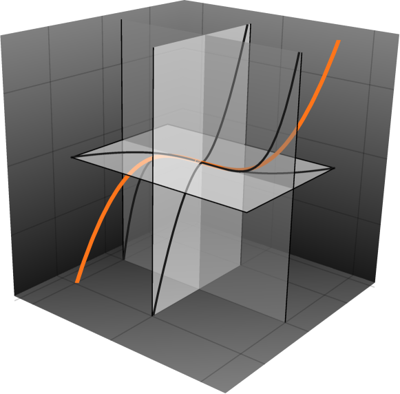
Figure 1: The curve $\Gamma$ of Example 4.4 together with its planar projections $\Gamma_{1,2}$, $\Gamma_{2,3}$, and $\Gamma_{1,3}$.

References

• [1] S. Bartz and S. Reich, Abstract convex optimal antiderivatives, Annales de l’Institut Henri Poincare (C) Non Linear Analysis 29 (2012), 435–454.
• [2] S. Bartz and S. Reich, Optimal pricing for optimal transport, Set-Valued and Variational Analysis 22 (2014), 467–481.
• [3] H.H. Bauschke and P.L. Combettes, Convex Analysis and Monotone Operator Theory in Hilbert Spaces, Springer, 2011.
• [4] M. Beiglböck and C. Griessler, An optimality principle with applications in optimal transport, arXiv preprint, arXiv:1404.7054 (2014).
• [5] H. Brezis, Liquid crystals and energy estimates for $S^{2}$-valued maps, Theory and Applications of Liquid Crystals (Minneapolis, Minn., 1985), The IMA Volumes in Mathematics and its Applications Volume 5, Springer, (1987), 31–52.
• [6] G. Carlier, On a class of multidimensional optimal transportation problems, Journal of Convex Analysis 10 (2003), 517–529.
• [7] G. Carlier and B. Nazaret, Optimal transportation for the determinant, ESAIM: Control, Optimisation and Calculus of Variations 14 (2008), 678–698.
• [8] L. Debnath and P. Mikusiński, Introduction to Hilbert Spaces with Applications, 3rd edition, Academic Press, 2005.
• [9] S. Di Marino, L. De Pascale and M. Colombo, Multimarginal optimal transport maps for 1-dimensional repulsive costs, Canadian Journal of Mathematics 67 (2015), 350–368.
• [10] S. Di Marino, A. Gerolin and L. Nenna, Optimal transportation theory with repulsive costs, arXiv preprint (2015), arXiv:1506.04565.
• [11] W. Gangbo and R. McCann, The geometry of optimal transportation, Acta Mathematica 177 (1996), 113–161.
• [12] W. Gangbo and A. Swiech, Optimal maps for the multidimensional Monge-Kantorovich problem, Communications on Pure and Applied Mathematics 51 (1998), 23–45.
• [13] N. Ghoussoub and B. Maurey, Remarks on multi-marginal symmetric Monge-Kantorovich problems, Discrete and Continuous Dynamical Systems 34 (2013), 1465–1480.
• [14] N. Ghoussoub and A. Moameni, Symmetric Monge-Kantorovich problems and polar decompositions of vector fields, Geometric and Functional Analysis 24 (2014), 1129–1166.
• [15] C. Griessler, $c$-cyclical monotonicity as a sufficient criterion for optimality in the multi-marginal Monge-Kantorovich problem, arXiv preprint (2016), arXiv:1601.05608.
• [16] H.G. Kellerer, Duality theorems for marginal problems, Zeitschrift für Wahrscheinlichkeitstheorie und Verwandte Gebiete 67 (1984), 399–432.
• [17] Y.-H. Kim and B. Pass, A general condition for Monge solutions in the multi-marginal optimal transport problem, SIAM Journal on Mathematical Analysis 46 (2014), 1538–1550.
• [18] M. Knott and C.S. Smith, On a generalization of cyclic monotonicity and distances among random vectors, Linear Algebra and its Applications 199 (1994), 363–371.
• [19] A. Moameni and B. Pass, Solutions to multi-marginal optimal transport problems concentrated on several graphs, ESAIM: Control, Optimization and Calculus of Variations (2015), in press.
• [20] B. Pass, On the local structure of optimal measures in the multi-marginal optimal transportation problem, Calculus of Variations and Partial Differential Equations 43 (2012), 529–536.
• [21] B. Pass, Multi-marginal optimal transport: theory and applications, ESAIM: Mathematical Modelling and Numerical Analysis 49 (2015), 1771–1790.
• [22] F. Riesz and B. Sz.-Nagy, Leçons d’Analyse Fonctionnelle, cinquième, Gauthier-Villars, 1968.
• [23] J.-C. Rochet, A necessary and sufficient condition for rationalizability in a quasilinear context, Journal of Mathematical Economics 16 (1987), 191–200.
• [24] R.T. Rockafellar, Characterization of the subdifferentials of convex functions, Pacific Journal of Mathematics 17 (1966), 497–510.
• [25] L. Rüschendorf, On $c$-optimal random variables, Statistics and Probability Letters 27 (1996), 267–270.
• [26] F. Santambrogio, Optimal Transport for Applied Mathematicians, Birkhäuser, 2015.
• [27] C. Villani, Optimal Transport: Old and New, Springer, 2009.