UTTG-14-16, KCL-PH-TH/2016-53
Robustness of Inflation to Inhomogeneous Initial Conditions
Abstract
We consider the effects of inhomogeneous initial conditions in both the scalar field profile and the extrinsic curvature on different inflationary models. In particular, we compare the robustness of small field inflation to that of large field inflation, using numerical simulations with Einstein gravity in 3+1 dimensions. We find that small field inflation can fail in the presence of subdominant gradient energies, suggesting that it is much less robust to inhomogeneities than large field inflation, which withstands dominant gradient energies. However, we also show that small field inflation can be successful even if some regions of spacetime start out in the region of the potential that does not support inflation. In the large field case, we confirm previous results that inflation is robust if the inflaton occupies the inflationary part of the potential. Furthermore, we show that increasing initial scalar gradients will not form sufficiently massive inflation-ending black holes if the initial hypersurface is approximately flat. Finally, we consider the large field case with a varying extrinsic curvature , such that some regions are initially collapsing. We find that this may again lead to local black holes, but overall the spacetime remains inflationary if the spacetime is open, which confirms previous theoretical studies.
I Introduction
Cosmic Inflation Guth (1981); Linde (1982); Albrecht and Steinhardt (1982); Starobinsky (1980) is thought to provide a solution to several problems in standard Big Bang theory by dynamically driving a “generic” initial state to a flat, homogeneous and isotropic Universe, while generating a nearly scale-invariant power spectrum of primordial perturbations which is consistent with observations. The question of what constitutes a “generic” initial state is a difficult one, and can only be understood in the context of a quantum theory of gravity. However, regardless of the nature of quantum gravity, a random realisation from the set of all possible initial conditions will not look like an inflationary spacetime, and one should expect the initial conditions from which inflation begins to contain some measure of inhomogeneity.
Inhomogeneities do not necessarily prevent inflation in models of chaotic inflation Linde (1983) where inflation may naturally begin near the Planck scale Linde (1984, 1985, 2015). However, the simplest models of chaotic inflation in which inflation can start at the Planck scale are under pressure from recent observations of the cosmic microwave background Ade et al. (2016). The data does not exclude scenarios in which inflation begins near the Planck scale Mukhanov (2013); Kallosh et al. (2014), but it motivates a study of the effects of inhomogeneities on scenarios in which the potential energy density is always sub-Planckian. While inflation in this class of models may start naturally if the topology of the spatial slices of our universe is non-trivial Linde (2004), or if the cores of topological defects serve as seeds Linde (1994); Vilenkin (1994); Linde and Linde (1994), the effects of inhomogeneities on the onset of inflation in these models in general is less understood and will be the focus of this work.
The issue of initial conditions for inflation and the stability of de Sitter and inflationary spacetimes have been under investigation for as long as inflation itself Linde (1983, 1985), and there are many analytic and semi-analytic Gibbons and Hawking (1977); Hawking and Moss (1982); Wald (1983); Starobinsky (1983); Barrow and Stein-Schabes (1984); Albrecht and Brandenberger (1985); Barrow and Tipler (1985); Gibbons et al. (1987); Jensen and Stein-Schabes (1987); Hawking and Page (1988); Penrose (1989); Muller et al. (1990); Kitada and Maeda (1992, 1993); Bruni et al. (1995); Maleknejad and Sheikh-Jabbari (2012); Gibbons and Turok (2008); Boucher and Gibbons (2011); Bruni et al. (2002); Muller et al. (1988); Barrow and Goetz (1989); Bicak and Podolsky (1997); Capozziello et al. (1998); Vachaspati and Trodden (1999); Barrow (1987, 1986); Polyakov (2010); Marolf and Morrison (2011); Tsamis and Woodard (1993); Brandenberger (2002); Geshnizjani and Brandenberger (2005); Marozzi et al. (2013); Brandenberger and Kung (1990); Carroll and Tam (2010); Corichi and Karami (2011); Schiffrin and Wald (2012); Remmen and Carroll (2013); Corichi and Sloan (2014); Mukhanov (2015); Remmen and Carroll (2014); Berezhiani and Trodden (2015); Kleban and Senatore (2016) as well as numerical studies Albrecht et al. (1985, 1987); Kurki-Suonio et al. (1987); Feldman and Brandenberger (1989); Brandenberger and Feldman (1989); Goldwirth and Piran (1990, 1989); Brandenberger et al. (1991); Laguna et al. (1991); Goldwirth and Piran (1992); Kurki-Suonio et al. (1993); Easther et al. (2014); East et al. (2016); Braden et al. (2016); Alho and Mena (2011, 2014) (see Brandenberger (2016) for a short review). Goldwirth and Piran Goldwirth and Piran (1990, 1989, 1992) were the first to study the robustness of inflation to spherically symmetric perturbations using general relativistic 1+1D simulations.111An earlier pioneering work Albrecht et al. (1985) showed that inhomogeneous scalar fields will homogenise in a fixed FRW background. See also Easther et al. (2014) for a recent follow up work in this direction. In modern terminology, their conclusion was that large field models, in which the inflaton traverses more than a Planck mass during the inflationary period, , are more robust than small field models, . Their results are often taken to imply that inflation requires a homogenous patch of size roughly to begin. This work was later followed by 3+1D numerical simulations in Refs. Kurki-Suonio et al. (1993); Laguna et al. (1991) showing large field inflation to be robust to simple inhomogeneous (and anisotropic) initial conditions with large initial gradient energies in situations in which the field is initially confined to the part of the potential that supports inflation. This was confirmed recently in Ref. East et al. (2016), which demonstrated that large field inflation is robust even if where is the vacuum energy density, at least if the universe initially expands at the same rate everywhere. Furthermore, East et al. (2016) first presented simulations in which inflation succeeded even for certain initial conditions that lead to the formation of black holes.
In this paper, we continue this line of research and test the robustness of inflation to a slightly more general but still very simple class of inhomogeneous initial conditions both in the scalar field profile and the extrinsic curvature. We use the numerical relativity package Clough et al. (2015), setting up the machinery that will allow us to study more general classes of initial conditions in the future. Since the degree of robustness to inhomogeneities depends on the exact model of inflation, this provides us with an approach to checking model viability. According to the Lyth bound Lyth (1997); Turner (1997), inflation occurs at high energies and involves large field excursions in models that produce observable amounts of primordial gravitational waves, whereas the energy scale and field excursion are small in models that do not. Our results are summarized as follows:
- •
-
•
Small field inflation is less robust than large field inflation. It can fail even when the energy density in gradients is subdominant . We show that small field inflation fails when a large enough local fluctuation ends inflation early in that particular region, with the gradients quickly dragging the rest of the spacetime from the inflating part of the potential. However, the size of local fluctuation required to end inflation must be large enough to explore the boundary of inflationary regime of the potential, making small field inflation somewhat more robust than might be expected.
-
•
Large inhomogeneities do not form dominant black hole spacetimes. In the large field case, the potential is sufficiently wide to support inhomogeneities which result in collapse to form black holes. However, in the case where the initial spacetime is flat on average, increasing gradient energy implies an increase in average initial expansion. This expansion prevents the formation of inflation-ending black hole spacetimes. We found that there exists a maximum black hole mass which is subdominant to the inflationary spacetime, which we derived both analytically and numerically.
-
•
We show that for initial spacetimes containing both expanding and collapsing regions local regions may collapse into black holes. However, inflation will occur as long as the spacetime is on average initially expanding. This is consistent with the theoretical expectations of Barrow and Tipler (1985) and Kleban and Senatore (2016).
This paper is organised as follows. In Section II we present the theory and methodology of our approach. In Sections III and IV, we present the numerical results, and discuss their implications for the small field and large field cases respectively. We conclude in Section V.
Movies of several of the simulations described in this paper can be accessed via the website at http://grchombo.org.
II Theory and Methodology
We consider single-field inflation with canonical kinetic term
| (1) |
For a spatially homogeneous configuration, inflation occurs if and the slow-roll parameters satisfy
| (2) |
with . In this case the field is slowly rolling and acts as a cosmological constant resulting in an inflating spacetime. The second condition is required to ensure that inflation occurs for the sufficient amount of e-foldings.
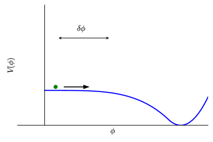
In the large-field models, the region of the potential where this occurs is super-Planckian, i.e. the field needs to roll for sufficient inflation, while in the small field model the field traverses a sub-Planckian distance in field space . This is illustrated in Figure 1. In the context of single field inflation, the Lyth bound Lyth (1997) implies that high/low-scale inflation is associated with large/small field inflation.
II.1 Initial Conditions
We impose very simple inhomogeneous initial conditions similar to those in East et al. (2016) by specifying the initial condition for the scalar field as follows
| (3) |
and
| (4) |
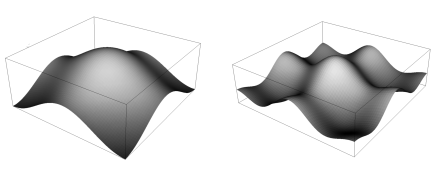
where is the spatial coordinate of a foliation labeled by the time coordinate , and is the amplitude of the initial inhomogeneities. The value is chosen such that we have 100 e-folds of inflation in the absence of any inhomogeneities. Since there are three modes each with amplitude , the maximal total amplitude of the fluctuations about is . We chose not to include random phases in this work as we have found that random phases do not materially change the overall results. Note that we have normalised the total by the number of modes – this means that the average gradient energy is slightly higher for larger , but that the maximum traverse from towards the inflationary minimum is the same. See Figure 2 for an illustration of the cases and .
We set to be the length of the simulation domain, and use periodic boundary conditions to simulate a space composed of periodic fluctuations of this length and amplitude. is chosen to be the Hubble length in the absence of inhomogeneities (), that is
| (5) |
Hence, our model of initial inhomogeneities depends on the integer , the amplitude of inhomogeneities , and the potential . The potential sets the inflationary Hubble scale, the integer sets the wavelength of the shortest perturbations relative to this scale, and sets the amplitude of the inhomogeneities. In this work we focus on of order unity and leave a more systematic study of the space of initial conditions for future work. In large field inflation we use a single mode, i.e. , and vary . In the limit in which the gradient energy dominates, i.e. , changing is equivalent to changing the wavelength of the mode relative to the actual Hubble length (including the energy density from fluctuations). For and a Euclidean metric on the initial slice the wave number satisfies
| (6) |
In small field inflation, we consider the two cases , and , a superposition of two modes, in addition to the variation of . We will see that already small prevent successful inflation in the small field case so that we are not in the regime .
We use the ADM metric, following the conventions of Clough et al. (2015),
| (7) |
where and are the lapse and shift parameters as usual. In the BSSN formalism of numerical relativity Baumgarte and Shapiro (1999); Shibata and Nakamura (1995), these parameters are specified on the initial hypersurface and then allowed to evolve using gauge-driver equations. We choose and on the initial hypersurface, and hence the initial gradient energy on this hypersurface is
| (8) |
It is convenient to introduce the conformal metric such that , the corresponding Christoffel-symbols , as well as the short-hand notation . We can then write the equations we use to evolve the lapse and shift in the moving puncture gauge van Meter et al. (2006); Campanelli et al. (2006), which allows us to stably form and evolve black holes in the spacetime, as
| (9) | |||||
| (10) | |||||
| (11) |
The exact values of and are chosen to improve stability in any particular numerical simulation.
Next, we have to specify the initial conditions for the metric and extrinsic curvature . Their values need to satisfy both the Hamiltonian and momentum constraints on the initial hypersurface. Decomposing the extrinsic curvature as
| (12) |
and introducing the notation for the kinetic term
| (13) |
so that the energy density at any point in the hypersurface is
| (14) |
the constraint equations become
| (15) |
and
| (16) |
is the local expansion rate of spacetime, and in the special case of the Friedmann-Robertson-Walker metric, where is the Hubble constant.222Note that we have chosen convention such that denotes positive expansion.
This is a set of coupled elliptic equations and is non-trivial to solve in general. Throughout this work, we will make the simplifying assumption that the metric is conformally flat and the traceless part of the extrinsic curvature is zero everywhere on the initial slice
| (17) |
and
| (18) |
In this special class of initial conditions, we consider two possible solutions, that of uniform initial expansion , and one with spatially varying .
II.1.1 uniform initial expansion
For spatially varying , the momentum constraint Eqn. (16) is trivially satisfied for and const. is in principle a free parameter, corresponding to a uniform local expansion rate across the initial hypersurface. However, in order to satisfy periodic boundary conditions for and the Hamiltonian constraint, needs to lie close to the average initial energy density for the hypersurface. For simplicity, we choose it to be equal to the average initial energy density, approximating the metric to be Euclidean
| (19) |
with
| (20) |
where indicates the average over the spatial volume of the quantity . Once is chosen, the initial field profile and the Hamiltonian constraint then fully determine the conformal factor (which we solve for using numerical relaxation).
In cases where the gradient energy dominates i.e. , the initial expansion rate is large compared to the Hubble rate associated with inflation. This large initial uniform expansion means that we are stacking the deck against ending inflation. In general, we should expect the local expansion rate to be a function of spatial position that can be both initially expanding or collapsing. To study the general case will require relaxing some combination of the conformal condition Eqn. (17), the condition on , Eqn. (18), and the condition of zero initial scalar field velocity, . We reserve the general case for future work, but there exists a second solution consistent with equations (17) and (18), given our assumptions, from imposing , which gives non-uniform initial expansion. We turn to this solution next.
II.1.2 expanding/contracting initial condition
For constant initial scalar velocity
| (21) |
with some constant, the momentum constraint Eqn. (16) relates the extrinsic curvature to the initial scalar field profile
| (22) |
where is an integration constant. This initial condition means that a constant initial scalar velocity and a varying field will lead to a spatially varying . If is chosen to be approximately the average value of , the spacetime will be locally initially expanding or contracting depending on its position. We can then again solve the Hamiltonian constraint for the conformal factor in order to complete the specification of the initial conditions.
II.2 Numerical Set-up
We rescale our simulations (by choosing the geometrized mass unit to represent some convenient fraction of ) such that the size of our physical domain is covered by . We turn on ’s adaptive mesh refinement, using the gradients of and as refinement threshold conditions, with a coarsest level grid size of , allowing up to 6 of levels of refinement with a refinement ratio of per level. We check convergence approximately in this case by checking that the same results are obtained when starting from a coarsest grid of , increasing the number of grids by one and using a more aggressive regridding condition (approximately halving the thresholds). It was found that the difference in the results was small – for example, the number of -folds at failure in the small field cases were different by .
We can track inflationary simulations for around 23 -folds. After this point numerical error begins to dominate as the conformal factor (equal to the inverse of the square of the scale factor) falls below working precision.
III Small Field Inflation
As discussed in the Introduction, the inflating plateau of the small field potential can be relatively narrow, with . The reason is as follows. The scalar power spectrum for single field inflation is given by
| (23) |
For low scale inflation is small, which means that must be small to achieve sufficient amplification of the observed scalar power. This means that the inflaton has to be roll very slowly (when compared to the large field case). The number of e-folds , is given by
| (24) |
Assuming and constant, we estimate the field range with the help of equation (23)
| (25) |
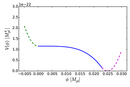
For a typical low scale inflation , we see that so is sub-Planckian as we argued. A typical small field inflation model is shown in Fig. 3, where the inflating domain is around the inflection point of the potential.
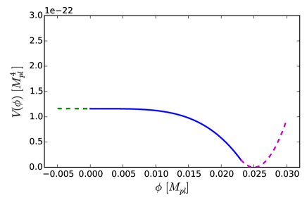
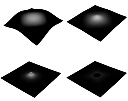
Inflation could occur for much longer than 60 -folds. Therefore the inflection point could be quite broad, while still accommodating the small field requirement, so the potential could instead look like Figure 4, with a wider plateau. In the context of inhomogeneous inflation, this distinction is important – the presence of large gradients means that the scalar field can now sample a large domain of the potential, which could include the non-inflating “cliff” on the left side of the potential in Figure 3. The additional potential energy in such regions is converted to scalar kinetic energy as the field rolls down the hill towards the inflection point, which can disrupt slow roll sufficiently to end inflation.
In this section, we will explore and compare the two cases, a potential with an extended flat direction, and one with a steeper rise. Note that we do not consider the effect of varying on small field inflation. This is because a profile for which covers both negative and positive values (i.e. with both expanding and contracting regions), requires the addition of a relatively large kinetic energy term , which immediately pushes the field into the minimum, ending inflation. Thus the case where is constant represents a best case scenario – adding variation in will only end inflation sooner. This is consistent with initial kinetic energy being the most important failure mode, as shown by Goldwirth and Piran.
III.1 Small Field model with extended flat direction
In this section, we will investigate the robustness of small field inflation for the case depicted in Figure 4.
We model the inflationary potential as
| (26) |
with , , and . The Hubble rate during inflation for this choice of parameters is .
For a homogeneous initial value of the field of , these values would result in 100 e-folds of inflation, and for modes that exit the horizon 60 -folds before the end of inflation. We find the end of the inflationary plateau, the point at which the potential is no longer “slow roll”, to be at approximately , with all but the last -fold taking place for .
The length scale for the fluctuations , set to the Hubble length in the absence of fluctuations, is then , and the value of is constant across the grid as described in section II. This satisfies the Hamiltonian constraint, assuming that the initial value of the conformal factor of the metric, , is approximately of order 1. In our simulations, we set this constant value of across the grid and then relax the value of from a value of 1 everywhere to satisfy the Hamiltonian constraint exactly.333Although in the small field case remains very close to 1 as the fluctuations are small, and the space is approximately flat.
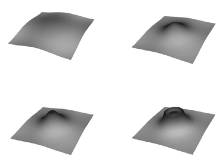
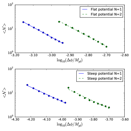
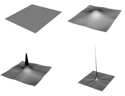
We then evolve the initial conditions forward in time until inflation ends, or we reach the maximum number of -folds we can simulate. We define the end of inflation as being the point at which a single point in the space falls to the minimum of the potential, that is, when the value of somewhere on the grid. The rest of the space will subsequently be pulled in by gradients, as illustrated in Figure 5, and as we will discuss in more detail in the next section. The average number of -folds is measured on this time slice.444While the remaining spacetime can achieve several more e-folds before falling to the minimum, we treat this point as having ended inflation for measurement purposes. Allowing the simulations to run until the whole spacetime has fallen to the minimum and fully ceased inflating would displace the lines in Figure 6 vertically, but the trends would be the same. The actual values of are, in any case, model specific. We do this for a range of . The results are shown in Figure 6 for the cases and .
For we find that inflation ends with less than 20 e-folds (which we call “failure” for our purposes) for initial amplitudes of around . These values of correspond to .555This implies that we are in a very different regime in our simulations of small-field models from East et al. (2016) where the gradient energy density dominated the potential energy density in both the large- and small-field case. We find that already subdominant energy density in gradients can significantly impede or prevent inflation. Hence the gradient energy is still sub-dominant to the length scale . This is highly “homogenous”. Note that the density contrast in inflationary primordial perturbations are expected to be of order which is only an order of magnitude smaller than this. However, the perturbations here are concentrated in one or two modes and it is the field excursions that should be compared. The typical displacement due to quantum fluctuations is . We will explore the robustness of inflation to initial perturbations with more general power spectra in future work.
For we find failure when . It can be seen that adding the additional mode makes inflation more robust. Recall from the definition Eqn. (3) that we have normalised to the total number of modes so adding modes adds to the gradient energy but not to the maximum field value – this suggests that inflationary failure scenarios are more dependent on single long wavelength inhomogeneities rather than multiple short wavelength ones. The number of -folds decreases with an approximate relationship of in both the and cases.
III.2 Pull back effects in small field inflation
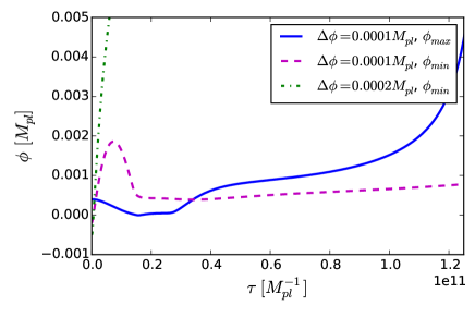
As was mentioned above, once one part of the field falls into the minimum, it quickly “drags down” the remaining spacetime, as shown in Figure 5. It is instructive to consider the scalar field dynamics which leads to the failure as the naive expectation that the part of the field which has the maximum initial value (and hence is closer to the point where inflation ends) is that which falls to the minimum first is not always correct. There is some initial resistance from gradient pressure which, for a range of , pulls the field back up the hill away from the minimum, “saving” inflation and making it more robust to inflation than one might expect. See Figure 7.
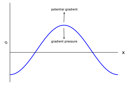
Using the Klein-Gordon equation, we can show that local gradient pressure should temporarily “save” inflation up to some critical value, above which the field will fall directly to the minimum. The critical value for where this happens can be approximated quite accurately as follows. Consider the Klein-Gordon equation,
| (27) |
where we have ignored the friction term, and let
| (28) |
Initially, and . For this point, and assuming that we are still in the concave part of the potential, the field value should fall initially towards the minimum if
| (29) |
For the initial conditions and the potential we consider, this is the case (assuming ) for
| (30) |
Using the relation Eqn. (5), , and for our small field case this becomes
| (31) |
which simplifies to
| (32) |
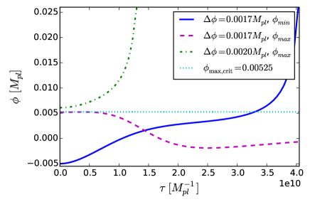
The critical value for our chosen values and is , which corresponds to , beyond the part of the potential that supports an extended period of inflation. Small field inflation is thus more robust than on might naively expect because local excursions towards the edge of the inflationary plateau are pulled back onto it.
The results of several simulations are illustrated in Figure 8. We see that the predicted critical value for at which immediate failure occurs is approximately correct. In fact the field can even resist some initial movement towards the minimum at the maximum point, before being pulled back up the potential hill.
III.3 Small Field model without extended flat direction
In this section, we will investigate the robustness of small field inflation in the case in which the negative direction is a “cliff”. We model the potential as
| (33) |
with the same parameters and initial conditions as in Section III.1. The is illustrated in Figure 3.
For the case, we find failure for initial amplitudes of , which corresponds to . Note that inflation now fails for amplitudes roughly an order of magnitude smaller than in the case of the extended flat region, showing that small field inflation is highly sensitive to changes in the potential around the flat region. Although the energy density in these fluctuations is now smaller than those expected from inflationary primordial perturbations, recall that it is concentrated in one mode, rather than being a scale invariant spectrum. In particular, the typical displacement due to quantum fluctuations for a given mode is still significantly smaller than the fluctuations considered here .
The results are shown in Figure 6 for the cases and , below those for the case with the flatter potential. Again it can be seen that adding the additional mode makes inflation slightly more robust. The number of -folds decreases as a power law with an approximate relationship of .
In this case the dynamics of the failure is driven by the most positive point. One might expect the most negative point to rapidly gain kinetic energy and overshoot the inflationary plateau, but this is only observed for higher values of and for small the field is “pulled back” by the gradients in the field. The most positive point in this case gets pulled back as before, but then hits the steep “wall” and proceeds to roll off the plateau. This is illustrated in Figure 9.
Again thinking solely about the scalar field dynamics of the extremal points, one can estimate at which point the most negative point will fail directly. Consider the most negative value of initially, . We can see that it will fail if, having oscillated through , the point at which it would be brought to rest by gradient pressure exceeds the critical point derived in the previous section of . If the potential were flat in this region, this value would be the same as (since it is effectively in simple harmonic motion). However, the initial slope in gives it an extra “push”, which we can equate to having started with a larger value of . Considering the initial energy density at the minimum point, relative to the point
| (34) |
then by making the approximations and , this becomes
| (35) |
and we can find an “effective” initial value of , which would have the same initial energy density
| (36) |
Setting this equal to gives a rough estimate for the initial value of leading to immediate failure at the minimum point, which using our specific values gives . As shown in Figure 9, this value is consistent with our findings, although failure will occur slightly below this value, due to the various assumptions made, in particular that the potential is flat after , when it is in fact sloped downwards.
IV Large Field Inflation
In large field inflation the inflationary part of the potential is . It thus supports larger fluctuations in the field while still keeping the entire space within the inflationary regime.
Work to test the robustness of inflation in large field inflation was done in Kurki-Suonio et al. (1993), and more recently by East et al. (2016) who found that large field inflation with uniformly expanding initial conditions is very robust to large inhomogeneities of up to . In this section we broadly reproduce their results, before extending the work to consider the limit of very large fluctuations and non-uniform initial expansion rates which include initially contracting regions.
We use inflation as a generic model for large scale inflation666While this model is marginally ruled out by the latest Planck data Ade et al. (2015), we chose it for its simplicity of implementation. More complicated models will not lead to any drastically different results since the key feature is the flatness of the potential and the long traverse to the minimum.
| (37) |
with , leading to an inflationary scale of . For an initial value of the field of , these values would result in 100 e-folds of inflation, with the scalar perturbation amplitude and the scalar index for modes that exit the horizon 60 -folds before the end of inflation.
The length scale for the fluctuations is set to the Hubble length in the absence of fluctuations, for our choice of parameters .
IV.1 Large field inflation with constant
In this section the value of , the extrinsic curvature, is set as a constant across the grid using Eqn. (19) as above. We first considered a range of initial amplitudes of the perturbations , and found that values below resulted in inflation everywhere.
We find that at larger values of , we form black holes. As in East et al. (2016), we can argue for their formation at this scale using the hoop conjecture. The black hole mass must be enclosed within a hoop of radius . Assuming spherical symmetry, this is
| (38) |
For a perturbation of wavelength , given that a single mode in each spatial direction necessarily creates two black holes by symmetry, the greatest radius from which each black hole can accrete is approximately
| (39) |
Note that, is an arbitrary length (the wavelength of the perturbation) and not necessarily the Hubble length. The mass enclosed, , is
| (40) |
where
| (41) |
which is obtained from the volume average of from Eqn. (3) over a volume . The maximum mass is then linearly proportional to , i.e.
| (42) |
Combining these gives the condition
| (43) |
as the critical case for black hole formation, independent of the length . This value of approximately is consistent with our findings above that the critical (given the approximate nature of the calculation).
Using equation Eqn. (6), this value of gives . This result is also consistent with the findings of East et al. (2016). In other words, black holes will form when the wavelength of the perturbation is four times the Hubble length or larger.
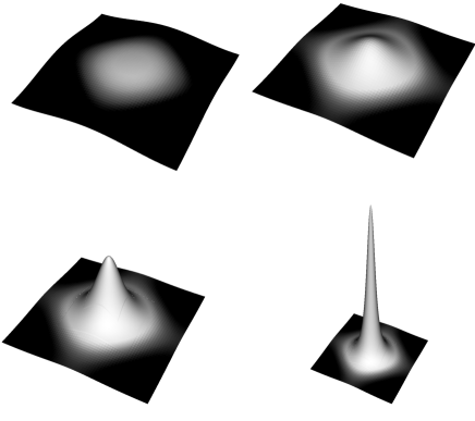
Above the critical value, black holes were formed, but these only created locally collapsing regions, and did not dominate the overall inflationary behaviour. As such they were quickly “inflated out” of the spacetime, see Figure 10.
The robustness was, as in the small field case, due in part to the fact that the most extreme value is quickly “pulled back” up the hill by gradient energy, resulting in initial inhomogeneities being smoothed out. For the potential we are using, and are both large and so the field will move towards the minimum when
| (44) |
which reduces to
| (45) |
Thus there is a minimum value beyond which pullback always occurs. This is because approaches zero at the minimum for type potentials – i.e. it is a convex potential. For concave type potentials (e.g. hill-top models Boubekeur and Lyth (2005)), there will be a maximum instead, as we have discussed in the small field case. The value of this bound is small, in our model , and in the limit of a very flat, extended potential, it is zero. Thus almost any perturbations will tend to be pulled back to a (potentially) more homogeneous configuration in this potential. This more homogeneous configuration then continues to inflate, with the number of e-folds approximately equal to that given by .
Thus, as expected, inflation eventually wins out, even with fluctuations which reach almost to the minimum of the potential – large field inflation is very robust to scalar field inhomogeneities.
IV.2 Can Black Holes stop inflation?
Naively, one might imagine that one can continuously increase the size of the fluctuations to generate black holes of increasing mass, to the point that the Schwarzschild radius dominates over the scale of inflation , ending inflation. The critical limit for this to occur is the so-called Nariai limit, which occurs when the black hole horizon and the de Sitter horizon coincide in a Schwarzschild-de Sitter spacetime. In our units, the critical mass of the black hole is
| (46) |
We will show in this section that this is not possible.
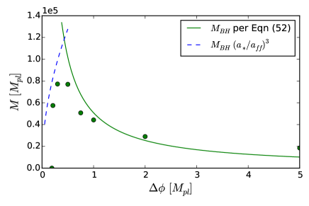
In Figure 11, we show the mass of the black holes formed as we gradually increase the amplitude obtained from numerical simulations. We see that while the mass increases with initially, at some point, the black hole mass begins to decrease as . Thus there is a maximum black hole mass which can be formed (which in our case had a Schwarzschild radius of about 20 per cent of the Hubble radius related to the initial , that is, ). This can be understood as follows.
Since initially, the early expansion of the spacetime is roughly that of a radiation dominated universe, i.e. and . At late times, the expansion rate is that of de Sitter, i.e. where .
Meanwhile, the free fall time-scale for some matter distribution of average density is given by
| (47) |
If there is no expansion, then this is roughly the timescale for some cloud of density to collapse to form a black hole as long as the initial distribution is supercritical. However, due to the presence of the large gradient energy density, the spacetime is roughly expanding as a radiation dominated universe, dissipating some of the energy away from forming a black hole. Once the spacetime is dominated by vacuum energy, it is safe to assume that any remaining energy that has not collapsed into a black hole will be rapidly dissipated. The time scale for this to happen, , occurs at vacuum-gradient energy equality , i.e.777Recall that in our conventions on the initial slice.
| (48) |
Converting into the scale factor by solving the Friedmann equation, we get
| (49) |
which is independent of as expected. This predicted value of provides a good approximation to the value of measured at black hole formation in the simulations over the range of tested. If , then de Sitter space will take over before the collapse has finished, leading to a lower mass black hole, and this is the case for smaller values of . By equating these two times from Eqn. (48) and Eqn. (49), we obtain
| (50) |
as the point when the free fall is no longer stopped by de Sitter expansion, resulting in a maximum mass of the black hole. This is in good agreement with the numerical value which gives the maximum mass at , as seen in Figure 11.
Above this point, the free fall timescale falls fully within the radiation dominated era. Consider the mass enclosed in a spherical distribution of matter of size
| (51) |
Since the collapse occurs well within the radiation domination era, the largest radius from which matter can still collapse into a black hole is the Hubble radius, , with the largest mass occurring when , giving us
| (52) |
which scales like as our numerical results indicate, and has a Schwarzschild radius of
| (53) |
which agrees to the maximum observed size of about for . This means that one cannot make a “Giant Death Black Hole” using the methods we outlined in this work – there is a maximum mass, roughly of the mass of the Nariai black hole Eqn. (46), after which increasing leads to a reduction in BH size. While our analysis and numerical simulations have focused on the specific case where the initial expansion is uniform and scaled to the gradient energy, we expect similar no-go results to hold as long as the initial hypersurface is approximately flat i.e. and since the Hamiltonian constraint Eqn. (15) implies that the initial expansion will be, on average, uniform and large. It would be interesting to revisit this question in the more general case where these assumptions are relaxed.
IV.3 Large field inflation with spatially varying
We now consider spatially varying in the case where and study the effect on inflation. The potential is now set to be simply a cosmological constant with the value from the previous large field case, to allow inflation to continue indefinitely.
For our purposes it is useful to recast Eqn. (22) for in the form
| (54) |
We set
| (55) |
where the value of now includes the contribution from . Without loss of generality, we set so that the maximum value of is zero for . Increasing increases the amplitude of the fluctuations in and allows us to consider larger regions of spacetime that are initially collapsing, . The profile for and the dependence on is illustrated in Figure 12.
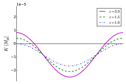
We test a range of values of between and , and find that in cases of smaller (where most of the spacetime is expanding initially) the collapsing part of the spacetime “bounces back”, such that quickly becomes approximately constant with a negative value everywhere. Inflation then continues, and over 20 efolds are reached.
In cases of higher , with , where more of the spacetime (but still less than half) is collapsing initially, we find that black holes form at the initially contracting point. We therefore find that for an inhomogeneous spacetime which would have resulted in inflation everywhere for constant ( is subcritical for black hole formation in the constant case), we are now able to generate regions of collapse to form black holes once variations of are introduced. This is illustrated in Figures 13 and 14.
However, even in these cases, the remaining spacetime continues to expand and inflate. Since in all cases here, this result is consistent with what would be expected from Barrow and Tipler (1985) and Kleban and Senatore (2016) (note that our sign convention means that denotes locally expanding spacetime). We will explore the case where in future work.
V Conclusions
We investigated the robustness of small and large field models of inflation, subjecting it to several simple inhomogeneous initial conditions both in the scalar field profile and in the extrinsic curvature. In doing so we have set up a framework that will allow us to study more general initial conditions in the future. As expected, we found that large field inflation was far more robust than small field inflation. In particular, small field inflation can fail even for small subdominant gradient energies while large field inflation is robust even to dominant gradient energies of . This implies that small field inflation requires at least some level of tuning to begin or a dynamical mechanism that sets up appropriate initial conditions.
V.1 Robustness of Small Field Inflation
The primary failure mode for small field inflation is the disruption of coherent slow roll dynamics, causing some parts of the scalar field to irrevocably fall into the non-inflating minimum. Once a region of the scalar field falls into the minimum, this region will expand and dominate the rest of spacetime ending inflation for the entire hypersurface. This failure mode can be induced in the following ways:
-
•
Adding large amplitude scalar fluctuations. Large amplitude scalar fluctuations can create excursions outside the inflationary part of the potential which lead to one region falling to the minimum and dragging the rest of the field down with it. However, local excursions of the field towards the edge of the inflationary part of the potential get pulled back by gradient pressure, making small field inflation more robust than one might expect (see below).
-
•
Converting additional potential energy into kinetic energy. If the inflationary region of the potential is small – in the case of typical small field models it is often just an inflection point – then a large initial fluctuation may have support on the steep part of the potential (i.e. the green dotted line in Figure 3). This additional potential energy will be converted to scalar kinetic energy, generating a large fluctuation and pushing the scalar closer to the minimum, thus ending inflation.
Nevertheless, we found that small field inflation is more robust than one might naively expect. In particular, we find the following:
-
•
Pullback effect of gradients. We show that perturbations tend to “homogenise”, i.e. gradients tend to flatten out. This means that some initial conditions which have regions in the non-inflating regime can still inflate as the scalar field gets pulled back into the inflating regime. We provide a formula for this critical point for any given potential, and demonstrate its effect numerically.
-
•
Adding additional shorter wavelength modes makes inflation more robust for a given maximum initial value of . Adding a second mode with half the wavelength, but normalised to keep the same value of , resulted in a higher threshold for inflation. This is somewhat unexpected since adding an mode increases the gradient energy. We proposed that this could be related to the pullback effect described above, which is stronger for higher wavenumber modes.
V.2 Robustness of Large Field Inflation
In the large field case, except for the trivial case of an initial hypersurface which is contracting everywhere, i.e. , we did not find a viable failure mode for the initial conditions we considered – large field inflation is robust to very large gradient energies . The primary reason for its robustness is the potential’s large support for slow roll i.e. , which combined with the rapid dissipation of gradient energy due to expansion, makes it difficult for the scalar to reach a non-inflating region. Furthermore, we find the following:
-
•
No “Giant Death Black Holes”. Given a uniformly expanding initial condition scaled to the total initial gradient energy, there is a maximum mass black hole that is formed for which the radius is of order times the size of the vacuum energy Hubble radius. Increasing initial gradients beyond this point decreases the final black hole mass – this is caused by the dissipation of gradient energies due to the large initial expansion. We calculate the maximum mass, which occurs when the transition to de Sitter expansion no longer limits the black hole mass, and confirm it with numerical simulations. We find that it is roughly of the mass of the Nariai black hole.
-
•
Pullback effect of gradients. Similar to the small field model, large gradients tend to homogenise. We show that for convex potentials, even with initial fluctuations which reach to the minimum of the potential, inflation can eventually succeed.
- •
As we stated in the Introduction, we only investigated a very restrictive class of initial conditions. Furthermore, we focused on the case of single field inflation. It will be interesting to study the effects of more general initial conditions and whether the presence of additional degrees of freedom renders inflation more or less robust to inhomogeneities. We will pursue these and other questions in future work.
Acknowledgements.
We thank Jonathan Braden, William East, Richard Easther, Matt Kleban, Hiranya Peiris, Matt Johnson, and Richard Matzner for useful conversations, and Robert Brandenberger for comments on our first draft. We would also like to thank the GRChombo team (http://grchombo.github.io/collaborators.html) for their work on the code, and various useful insights, and the COSMOS team at DAMTP, Cambridge for their ongoing technical support. Numerical simulations were performed on the COSMOS supercomputer, part of the DiRAC HPC, a facility which is funded by STFC and BIS. EAL acknowledges support from an STFC AGP grant ST/L000717/1. This work also used the ARCHER UK National Supercomputing Service (http://www.archer.ac.uk) for some simulations. BSD is supported in part by the National Science Foundation under grant PHY-1521186 and Maxwell Analytics LLC. BSD thanks the Helsinki Institute of Physics and the University of Amsterdam Institute for Theoretical Physics for their hospitality during part of this project. WF is supported by the National Science Foundation under Grant Number PHY-1316033. RF is supported in part by the Alfred P. Sloan Foundation. SP is grateful for support provided by the National Science Foundation under Grant Number PHY-1521186.References
- Guth (1981) A. H. Guth, Phys. Rev. D23, 347 (1981).
- Linde (1982) A. D. Linde, Second Seminar on Quantum Gravity Moscow, USSR, October 13-15, 1981, Phys. Lett. B108, 389 (1982).
- Albrecht and Steinhardt (1982) A. Albrecht and P. J. Steinhardt, Phys. Rev. Lett. 48, 1220 (1982).
- Starobinsky (1980) A. A. Starobinsky, Phys. Lett. B91, 99 (1980).
- Linde (1983) A. D. Linde, Phys. Lett. B129, 177 (1983).
- Linde (1984) A. D. Linde, Rept. Prog. Phys. 47, 925 (1984).
- Linde (1985) A. D. Linde, Phys. Lett. B162, 281 (1985).
- Linde (2015) A. Linde, in Proceedings, 100th Les Houches Summer School: Post-Planck Cosmology: Les Houches, France, July 8 - August 2, 2013 (2015) pp. 231–316, arXiv:1402.0526 [hep-th] .
- Ade et al. (2016) P. A. R. Ade et al. (BICEP2, Keck Array), Phys. Rev. Lett. 116, 031302 (2016), arXiv:1510.09217 [astro-ph.CO] .
- Mukhanov (2013) V. Mukhanov, Eur. Phys. J. C73, 2486 (2013), arXiv:1303.3925 [astro-ph.CO] .
- Kallosh et al. (2014) R. Kallosh, A. Linde, and A. Westphal, Phys. Rev. D90, 023534 (2014), arXiv:1405.0270 [hep-th] .
- Linde (2004) A. D. Linde, JCAP 0410, 004 (2004), arXiv:hep-th/0408164 [hep-th] .
- Linde (1994) A. D. Linde, Phys. Lett. B327, 208 (1994), arXiv:astro-ph/9402031 [astro-ph] .
- Vilenkin (1994) A. Vilenkin, Phys. Rev. Lett. 72, 3137 (1994), arXiv:hep-th/9402085 [hep-th] .
- Linde and Linde (1994) A. D. Linde and D. A. Linde, Phys. Rev. D50, 2456 (1994), arXiv:hep-th/9402115 [hep-th] .
- Gibbons and Hawking (1977) G. W. Gibbons and S. W. Hawking, Phys. Rev. D15, 2738 (1977).
- Hawking and Moss (1982) S. W. Hawking and I. G. Moss, Phys. Lett. B110, 35 (1982).
- Wald (1983) R. M. Wald, Phys. Rev. D28, 2118 (1983).
- Starobinsky (1983) A. A. Starobinsky, JETP Lett. 37, 66 (1983).
- Barrow and Stein-Schabes (1984) J. D. Barrow and J. Stein-Schabes, Phys. Lett. A103, 315 (1984).
- Albrecht and Brandenberger (1985) A. Albrecht and R. H. Brandenberger, Phys. Rev. D31, 1225 (1985).
- Barrow and Tipler (1985) J. D. Barrow and F. J. Tipler, MNRAS 216, 395 (1985).
- Gibbons et al. (1987) G. W. Gibbons, S. W. Hawking, and J. M. Stewart, Nucl. Phys. B281, 736 (1987).
- Jensen and Stein-Schabes (1987) L. G. Jensen and J. A. Stein-Schabes, Phys. Rev. D35, 1146 (1987).
- Hawking and Page (1988) S. W. Hawking and D. N. Page, Nucl. Phys. B298, 789 (1988).
- Penrose (1989) R. Penrose, 14th Texas Symposium on Relativistic Astrophysics Dallas, Texas, December 11-16, 1988, Annals N. Y. Acad. Sci. 571, 249 (1989).
- Muller et al. (1990) V. Muller, H. J. Schmidt, and A. A. Starobinsky, Class. Quant. Grav. 7, 1163 (1990).
- Kitada and Maeda (1992) Y. Kitada and K.-i. Maeda, Phys. Rev. D45, 1416 (1992).
- Kitada and Maeda (1993) Y. Kitada and K.-i. Maeda, Class. Quant. Grav. 10, 703 (1993).
- Bruni et al. (1995) M. Bruni, S. Matarrese, and O. Pantano, Phys. Rev. Lett. 74, 1916 (1995), arXiv:astro-ph/9407054 [astro-ph] .
- Maleknejad and Sheikh-Jabbari (2012) A. Maleknejad and M. M. Sheikh-Jabbari, Phys. Rev. D85, 123508 (2012), arXiv:1203.0219 [hep-th] .
- Gibbons and Turok (2008) G. W. Gibbons and N. Turok, Phys. Rev. D77, 063516 (2008), arXiv:hep-th/0609095 [hep-th] .
- Boucher and Gibbons (2011) W. Boucher and G. W. Gibbons, in Nuffield Workshop on the Very Early Universe Cambridge, England, June 21-July 9, 1982 (2011) pp. 273–278, arXiv:1109.3535 [astro-ph.CO] .
- Bruni et al. (2002) M. Bruni, F. C. Mena, and R. K. Tavakol, Class. Quant. Grav. 19, L23 (2002), arXiv:gr-qc/0107069 [gr-qc] .
- Muller et al. (1988) V. Muller, H. J. Schmidt, and A. A. Starobinsky, Phys. Lett. B202, 198 (1988).
- Barrow and Goetz (1989) J. D. Barrow and G. Goetz, Phys. Lett. B231, 228 (1989).
- Bicak and Podolsky (1997) J. Bicak and J. Podolsky, Phys. Rev. D55, 1985 (1997), arXiv:gr-qc/9901018 [gr-qc] .
- Capozziello et al. (1998) S. Capozziello, R. de Ritis, and A. A. Marino, Gen. Rel. Grav. 30, 1247 (1998), arXiv:gr-qc/9804053 [gr-qc] .
- Vachaspati and Trodden (1999) T. Vachaspati and M. Trodden, Phys. Rev. D61, 023502 (1999), arXiv:gr-qc/9811037 [gr-qc] .
- Barrow (1987) J. D. Barrow, Phys. Lett. B187, 12 (1987).
- Barrow (1986) J. D. Barrow, Phys. Lett. B180, 335 (1986).
- Polyakov (2010) A. M. Polyakov, Nucl. Phys. B834, 316 (2010), arXiv:0912.5503 [hep-th] .
- Marolf and Morrison (2011) D. Marolf and I. A. Morrison, Phys. Rev. D84, 044040 (2011), arXiv:1010.5327 [gr-qc] .
- Tsamis and Woodard (1993) N. C. Tsamis and R. P. Woodard, Phys. Lett. B301, 351 (1993).
- Brandenberger (2002) R. H. Brandenberger, in 18th IAP Colloquium on the Nature of Dark Energy: Observational and Theoretical Results on the Accelerating Universe Paris, France, July 1-5, 2002 (2002) arXiv:hep-th/0210165 [hep-th] .
- Geshnizjani and Brandenberger (2005) G. Geshnizjani and R. Brandenberger, JCAP 0504, 006 (2005), arXiv:hep-th/0310265 [hep-th] .
- Marozzi et al. (2013) G. Marozzi, G. P. Vacca, and R. H. Brandenberger, JCAP 1302, 027 (2013), arXiv:1212.6029 [hep-th] .
- Brandenberger and Kung (1990) R. H. Brandenberger and J. H. Kung, Phys. Rev. D42, 1008 (1990).
- Carroll and Tam (2010) S. M. Carroll and H. Tam, (2010), arXiv:1007.1417 [hep-th] .
- Corichi and Karami (2011) A. Corichi and A. Karami, Phys. Rev. D83, 104006 (2011), arXiv:1011.4249 [gr-qc] .
- Schiffrin and Wald (2012) J. S. Schiffrin and R. M. Wald, Phys. Rev. D86, 023521 (2012), arXiv:1202.1818 [gr-qc] .
- Remmen and Carroll (2013) G. N. Remmen and S. M. Carroll, Phys. Rev. D88, 083518 (2013), arXiv:1309.2611 [gr-qc] .
- Corichi and Sloan (2014) A. Corichi and D. Sloan, Class. Quant. Grav. 31, 062001 (2014), arXiv:1310.6399 [gr-qc] .
- Mukhanov (2015) V. Mukhanov, Fortsch. Phys. 63, 36 (2015), arXiv:1409.2335 [astro-ph.CO] .
- Remmen and Carroll (2014) G. N. Remmen and S. M. Carroll, Phys. Rev. D90, 063517 (2014), arXiv:1405.5538 [hep-th] .
- Berezhiani and Trodden (2015) L. Berezhiani and M. Trodden, Phys. Lett. B749, 425 (2015), arXiv:1504.01730 [hep-th] .
- Kleban and Senatore (2016) M. Kleban and L. Senatore, (2016), arXiv:1602.03520 [hep-th] .
- Albrecht et al. (1985) A. Albrecht, R. H. Brandenberger, and R. Matzner, Phys. Rev. D32, 1280 (1985).
- Albrecht et al. (1987) A. Albrecht, R. H. Brandenberger, and R. Matzner, Phys. Rev. D35, 429 (1987).
- Kurki-Suonio et al. (1987) H. Kurki-Suonio, R. A. Matzner, J. Centrella, and J. R. Wilson, Phys. Rev. D35, 435 (1987).
- Feldman and Brandenberger (1989) H. A. Feldman and R. H. Brandenberger, Phys. Lett. B227, 359 (1989).
- Brandenberger and Feldman (1989) R. H. Brandenberger and H. A. Feldman, Phys. Lett. B220, 361 (1989).
- Goldwirth and Piran (1990) D. S. Goldwirth and T. Piran, Phys. Rev. Lett. 64, 2852 (1990).
- Goldwirth and Piran (1989) D. S. Goldwirth and T. Piran, Phys. Rev. D40, 3263 (1989).
- Brandenberger et al. (1991) R. H. Brandenberger, H. Feldman, and J. Kung, Nobel Symposium 1990: The Birth and Early Evolution of the Universe Graftavallen, Sweden, June 11-16, 1990, Phys. Scripta T36, 64 (1991).
- Laguna et al. (1991) P. Laguna, H. Kurki-Suonio, and R. A. Matzner, Phys. Rev. D44, 3077 (1991).
- Goldwirth and Piran (1992) D. S. Goldwirth and T. Piran, Phys. Rept. 214, 223 (1992).
- Kurki-Suonio et al. (1993) H. Kurki-Suonio, P. Laguna, and R. A. Matzner, Phys. Rev. D48, 3611 (1993), arXiv:astro-ph/9306009 [astro-ph] .
- Easther et al. (2014) R. Easther, L. C. Price, and J. Rasero, JCAP 1408, 041 (2014), arXiv:1406.2869 [astro-ph.CO] .
- East et al. (2016) W. E. East, M. Kleban, A. Linde, and L. Senatore, JCAP 1609, 010 (2016), arXiv:1511.05143 [hep-th] .
- Braden et al. (2016) J. Braden, M. C. Johnson, H. V. Peiris, and A. Aguirre, (2016), arXiv:1604.04001 [astro-ph.CO] .
- Alho and Mena (2011) A. Alho and F. C. Mena, Phys. Lett. B703, 537 (2011).
- Alho and Mena (2014) A. Alho and F. C. Mena, Phys. Rev. D90, 043501 (2014), arXiv:1311.6348 [gr-qc] .
- Brandenberger (2016) R. Brandenberger, (2016), arXiv:1601.01918 [hep-th] .
- Clough et al. (2015) K. Clough, P. Figueras, H. Finkel, M. Kunesch, E. A. Lim, and S. Tunyasuvunakool, Class. Quant. Grav. 32, 245011 (2015), [Class. Quant. Grav.32,24(2015)], arXiv:1503.03436 [gr-qc] .
- Lyth (1997) D. H. Lyth, Phys. Rev. Lett. 78, 1861 (1997), arXiv:hep-ph/9606387 [hep-ph] .
- Turner (1997) M. S. Turner, Phys. Rev. D55, R435 (1997), arXiv:astro-ph/9607066 [astro-ph] .
- Baumgarte and Shapiro (1999) T. W. Baumgarte and S. L. Shapiro, Phys.Rev. D59, 024007 (1999), arXiv:gr-qc/9810065 [gr-qc] .
- Shibata and Nakamura (1995) M. Shibata and T. Nakamura, Phys.Rev. D52, 5428 (1995).
- van Meter et al. (2006) J. R. van Meter, J. G. Baker, M. Koppitz, and D.-I. Choi, Phys. Rev. D73, 124011 (2006), arXiv:gr-qc/0605030 [gr-qc] .
- Campanelli et al. (2006) M. Campanelli, C. O. Lousto, P. Marronetti, and Y. Zlochower, Phys. Rev. Lett. 96, 111101 (2006), arXiv:gr-qc/0511048 [gr-qc] .
- Ade et al. (2015) P. A. R. Ade et al. (Planck), (2015), arXiv:1502.02114 [astro-ph.CO] .
- Boubekeur and Lyth (2005) L. Boubekeur and D. Lyth, JCAP 0507, 010 (2005), arXiv:hep-ph/0502047 [hep-ph] .