Explaining Inverted Temperature Loops in the Quiet Solar Corona with Magnetohydrodynamic Wave Mode Conversion

Abstract

Coronal loops trace out bipolar, arch-like magnetic fields above the Sun’s surface. Recent measurements that combine rotational tomography, extreme ultraviolet imaging, and potential-field extrapolation have shown the existence of large loops with inverted temperature profiles; i.e., loops for which the apex temperature is a local minimum, not a maximum. These “down loops” appear to exist primarily in equatorial quiet regions near solar minimum. We simulate both these and the more prevalent large-scale “up loops” by modeling coronal heating as a time-steady superposition of: (1) dissipation of incompressible Alfvén-wave turbulence, and (2) dissipation of compressive waves formed by mode conversion from the initial population of Alfvén waves. We found that when a large percentage ($>$ 99%) of the Alfvén waves undergo this conversion, heating is greatly concentrated at the footpoints and stable “down loops” are created. In some cases we found loops with three maxima that are also gravitationally stable. Models that agree with the tomographic temperature data exhibit higher gas pressures for “down loops” than for “up loops,” which is consistent with observations. These models also show a narrow range of Alfvén wave amplitudes: 3 to 6 km s^-1 at the coronal base. This is low in comparison to typical observed amplitudes of 20 to 30 km s^-1 in bright X-ray loops. However, the large-scale loops we model are believed to comprise a weaker diffuse background that fills much of the volume of the corona. By constraining the physics of loops that underlie quiescent streamers, we hope to better understand the formation of the slow solar wind.

1. Introduction

Coronal loops are strands of closed magnetic field that fill much of the Sun’s outer atmosphere with hot plasma. Detailed simulations of loops are pivotal to understanding the physical processes responsible for coronal heating and the Sun’s overall magnetohydrodynamic (MHD) evolution. Early theoretical work employed constant heating rates as a function of distance along each loop (e.g., Rosner et al., 1978). Later classical coronal loop modeling introduced spatially varying heating rates from various sources but focused on short loops, often in active magnetic regions (Craig et al., 1978; Cargill & Priest, 1980; Wallenhorst, 1982; Steele & Priest, 1990; Orlando et al., 1995; Spadaro et al., 2003; Lundquist et al., 2008; Martens, 2010). Typically, these studies describe loops with temperatures that increase steadily from the chromosphere ($T\approx 10^{4}$ K) to the corona ($T\approx 10^{6}$ K). When longer loops were simulated with heating rates concentrated near their basal footpoints (Serio et al., 1981; Aschwanden & Schrijver, 2002), solutions were found with decreasing temperatures with increasing height in the vicinity of their apex. These loops were sometimes believed to be gravitationally or thermally unstable (Aschwanden et al., 2001), but they remained unobserved for some time.

Observations of loops in X-ray and ultraviolet wavelengths have tended to focus on the brightest and most collimated structures that stand out in contrast against a significantly dimmer diffuse coronal background. However, the recent development of differential emission measure tomography (DEMT; see Frazin et al., 2005, 2009; Vásquez et al., 2010, 2011) opened new perspectives on the measurement of plasma parameters in larger coronal structures. DEMT combines two techniques to achieve superior resolution: measurement of the coronal differential emission measure (DEM) distribution in three-dimensional space using solar rotational tomography (SRT). Multiple narrow-band images from the Atmospheric Imaging Array (AIA; Lemen et al., 2012) on the Solar Dynamics Observatory (SDO) were combined to determine the relative amounts of plasma at different temperatures along the optically thin line-of-sight. Tomographic techniques were then employed—assuming negligible coronal evolution over the time the Sun took to rotate through the full field of view—to extract the DEM information in each volume element. By tracing a field line provided by extrapolation of the coronal magnetic field from photospheric magnetograms and a Potential Field Source Surface (PFSS) model, the technique provides the mean electron density and electron temperature at various points in a tomographic grid. It then becomes possible to map out variations of temperature and pressure along individual large-scale closed field lines.

Huang et al. (2012) employed this technique to conduct one of the first major surveys of quiet-Sun loops. In the process, they discovered seemingly stable loops with negative temperature gradients near their apexes, which they labeled “down loops.” At nearly the same time, additional evidence for down loops was found from coronagraph measurements of line intensity ratios by Krishna Prasad et al. (2013). The DEMT results were expanded upon by Nuevo et al. (2013), who quantified the properties of several thousand loops in order to distinguish the down loops from the more common “up loops.”

This paper attempts to explain the results of Nuevo et al. (2013) by simulating large grids of coronal loops with heating mechanisms of varying strengths. We use time-steady rates of coronal heating in our models. There is considerable evidence for highly dynamic and time-dependent energy deposition in the corona (see, e.g., Aschwanden, 2006; Parnell & De Moortel, 2012; Klimchuk, 2015; Fletcher et al., 2015; Hansteen et al., 2015). However, the large, long-lived loops that are traceable using DEMT represent quasi-steady thermal states averaged over a relatively long time (i.e., several days). Thus, we believe it makes sense to consider similarly time-averaged heating rates in order to ascertain how that quasi-steady state is maintained. We make use of recent successes in modeling coronal heating via the nonlinear cascade of MHD turbulence, and we include the transfer of energy between incompressible (Alfvén) and compressible (magnetoacoustic) fluctuations.

In Section 2 we describe an empirically motivated way of modeling the shapes and magnetic properties of the large loops observed by Nuevo et al. (2013). Section 3 gives the relevant conservation equations for time-steady loops, and Section 4 discusses our adopted prescriptions for coronal heating. In Section 5 we describe the numerical methods used to solve for time-steady loop properties, the relevant boundary conditions, and the search for unstable solutions. Results for a large grid of loops are presented in Section 6, and we compare our models to the relevant observations. Finally, Section 7 contains a summary of our results and a discussion of implications for the overall coronal heating problem.

2. Loop Magnetic Fields

In many models of small coronal loops, the magnetic geometry is either simplified as a constant cross-section tube or as an expanding bundle of field lines with a specified function for the area expansion rate. For the large and often trans-equatorial loops considered in this paper, we aim to use a more realistic approach by modeling the spatial behavior of the vector magnetic field ${\bf B}$. Below we describe a semi-analytic “submerged monopole” model for coronal loop magnetic fields that is used in the coronal heating models below. We also describe how the parameters of this model are constrained by comparison with PFSS extrapolations of similar coronal conditions as observed by Nuevo et al. (2013).

When tracing along the magnetic field with a distance coordinate $s$ that follows the field lines, magnetic flux conservation constrains the field strength $B(s)$ to be inversely proportional to the cross-sectional area $A(s)$ of an idealized flux tube. For quiet-Sun loops far from active regions, we assume that the field can be approximated as the gradient of a potential. This allows us to construct the magnetic filed from the superposition of a number of point-like monopole sources beneath the solar surface. As long as the flux from positive sources is balanced by the flux from negative sources, the magnetic field above the surface will have $\nabla\cdot{\bf B}=0$. Thus,

$${\bf B}({\bf r})\,=\,\sum_{i}\frac{\Phi_{i}}{2\pi}\frac{{\bf r}-{\bf r}_{i}}{|{\bf r}-{\bf r}_{i}|^{3}}\,\,,$$ (1)

where the coordinates ${\bf r}_{i}$ specify the locations of each monopole source $i$, and the field point ${\bf r}$ can be located anywhere at or above the solar surface (see, e.g., Wang, 1998; Close et al., 2003). $\Phi_{i}$ is the signed magnetic flux in each source, and we require

$$\sum_{i}\Phi_{i}\,=\,0\,\,\,.$$ (2)

For simplicity, we use only two sources: one positive (located north of the equator) and one negative (south of the equator). Because our coronal heating model does not depend on the absolute magnitude of $B$, we consider the source fluxes $\Phi_{i}$ to be arbitrary and set them to $\pm 1$.

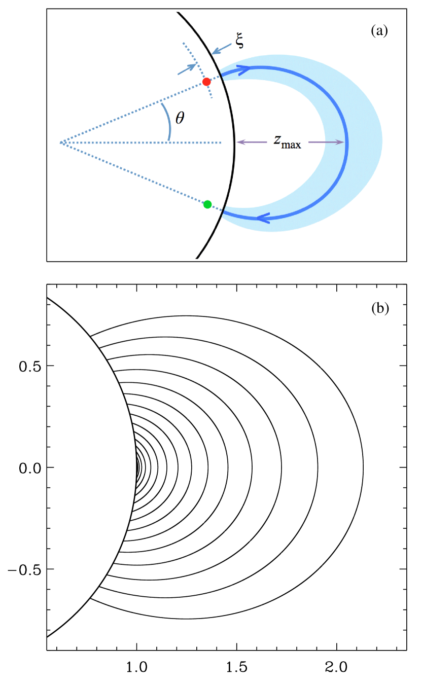
We constructed a grid of magnetic field properties for symmetric loops characterized by two free parameters: a footpoint latitude $\theta$ (i.e., half the angular separation between the two sources) and the submerged depth $\xi$ of each source. Figure 1(a) illustrates the geometry and the two parameters. Each choice of $\theta$ and $\xi$ describes a unique coronal loop with length $L$ (measured from one footpoint to the other), apex height $z_{\rm max}$ above the surface, and magnetic field ratio $B_{\rm max}/B_{\rm min}$ (where $B_{\rm max}$ is found at the surface and $B_{\rm min}$ is found at the apex). The local vector field B was traced along discrete steps of length $ds=1.5\times 10^{-3}\,R_{\odot}$ and tabulated. For symmetric fields, it is only necessary to trace the loop from one footpoint ($s=0$) to its apex ($s=L/2$).

Figure 1.— Illustration of the adopted loop geometry. (a) The loop length $L$ is measured from footpoint to footpoint along the dark blue magnetic field line. The monopole sources, submerged a distance $\xi$ beneath the surface, are denoted by red and green circles. (b) Loops computed with the $\xi(\theta)$ constraint of Equation (3). Increased values of $\theta$ lead to longer loops with greater values for the maximum distance to the surface $z_{\rm max}$.

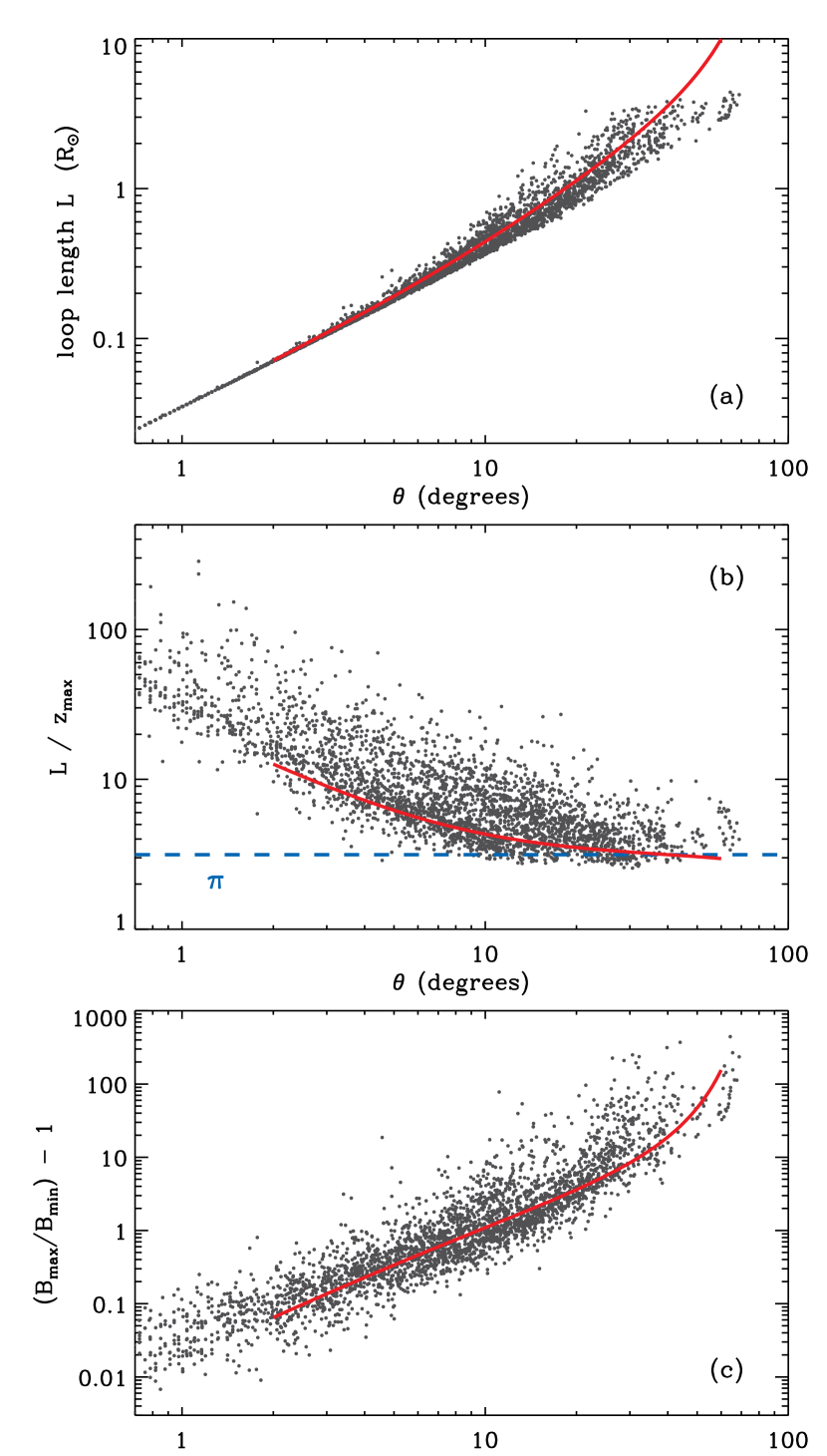
The full two-dimensional parameter space ($\theta$, $\xi$) of possible loops encompasses many unrealistic cases. In order to construct loops relevant to the actual quiet-Sun regions studied by Huang et al. (2012) and Nuevo et al. (2013), we found a single one-dimensional cut through the parameter space by constraining $\xi$ to be a function of $\theta$. We found this by comparing with coronal magnetic fields extrapolated from measured photospheric magnetograms with the PFSS technique. The PFSS method assumes the corona is current-free below a spherical “source surface” at $r=2.5\,R_{\odot}$, and that the field is pointed radially above it (Altschuler & Newkirk, 1969; Schatten et al., 1969). We used a low-resolution PFSS model made with synoptic magnetogram data from the Wilcox Solar Observatory (WSO; see Hoeksema & Scherrer, 1986). To best match the properties of the loops observed by Nuevo et al. (2013), we obtained PFSS coefficients for Carrington Rotations 2065, 2077, 2081, and 2106. These coefficients were constructed with maximum order $\ell=9$ in the spherical harmonic expansion. Following recent practice (e.g., DeRosa et al., 2012), we zeroed out all residual monopole ($\ell=0$) terms. For each rotation, we traced outwards from 500 random locations on the solar surface and kept track of only the closed loops. The trends observed in the loop geometries were consistent across numerous randomized sets.

Figure 2 shows some representative parameters as a function of $\theta$, which we measured from the PFSS model as half of the great-circle angle between each loop’s two footpoints. We searched for best relationship between $\theta$ and $\xi$ in the models described by Equation (1), and we found

$$\frac{\xi}{R_{\odot}}\,=\,0.27+\frac{2\theta}{\pi}$$ (3)

where $\theta$ is expressed in radians. Note that no single monotonic function $\xi(\theta)$ was able to reproduce “best-fitting” curves for each of the trends shown in Figure 2; the above relation is a compromise that appears to create reasonably realistic loops over the full range of observed lengths. Table 1 provides some basic data for a selection of loops that follows this pattern, and Figure 1(b) illustrates loop shapes for a subset of parameters. Note how the ratio $L/z_{\rm max}$ diverges from the idealized value of $\pi$ that one would expect for a semi-circular loop. The shortest loops are squat (i.e., $L/z_{\rm max}\gg\pi$) and the longest loops are stretched out radially ($L/z_{\rm max}\lesssim\pi$).

Figure 2.— (a) Model loop length $L$, (b) ratio of $L$ to the apex height $z_{\rm max}$, and (c) ratio of maximum to minimum magnetic field strength, all plotted versus footpoint latitude $\theta$. Black symbols show PFSS model properties from Carrington Rotations 2065, 2077, 2081, and 2106. Red curves show the result of applying Equation (3).

Table 1Geometric Properties of Quiet Sun Loops

$\theta$	$\xi$	$z_{\rm max}$	$L$	$B_{\rm max}/B_{\rm min}$
(deg)	($R_{\odot}$)	($R_{\odot}$)	($R_{\odot}$)	—
1	0.2811	0.0016	0.033	1.0187
2	0.2922	0.0059	0.069	1.0673
4	0.3144	0.0211	0.147	1.2328
8	0.3589	0.0711	0.333	1.7597
10	0.3811	0.1036	0.441	2.1018
12	0.4033	0.1402	0.561	2.4937
15	0.4367	0.2022	0.756	3.1797
20	0.4922	0.3242	1.134	4.6366
25	0.5478	0.4717	1.584	6.6300
30	0.6033	0.6499	2.121	9.4423
35	0.6589	0.8669	2.772	13.571
40	0.7144	1.1355	3.567	19.925
45	0.7700	1.4752	4.560	30.271

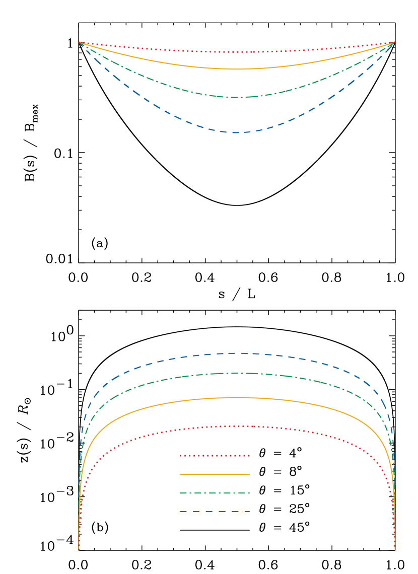
Figure 3 illustrates the variation of magnetic field strength $B$ and height $z$ as a function of $s$ for loops of various lengths. For a given loop configuration, the models need to know the relative variation of $A(s)\propto B(s)^{-1}$ and also how the height $z$ (and heliocentric radius $r=z+R_{\odot}$) depends on the loop-distance coordinate $s$.

Figure 3.— Distance dependence of (a) magnetic field strength $B$, in units of the maximum footpoint field strength $B_{\rm max}$, and (b) height $z$ above the photosphere. All properties are symmetric about the loop apex that occurs at $s=L/2$.

3. Conservation Equations

The plasma properties in the model coronal loops are computed under the assumptions of time independence, complete ionization, and hydrostatic equilibrium. We do not consider the properties of the underlying photosphere and chromosphere, and instead define the surface ($s=0$, $z=0$) at the base of the transition region (TR), with a fixed temperature $T_{0}$ and mass density $\rho_{0}$. Section 5.1 gives more details about the boundary conditions. We follow Schrijver & van Ballegooijen (2005) to specify the equation of state as

$$P=C_{1}n_{p}k_{\rm B}T\,\,,\,\,\,\,\,\,\,\,\,\,\,\,\rho=C_{2}n_{p}m_{p}\,\,,\,\,\,\,\,\,\,\,\,\,\,\,n_{e}=C_{3}n_{p}\,\,\,,$$ (4)

where $P$ is the gas pressure, $n_{p}$ is the proton density, $n_{e}$ is the electron density, $k_{\rm B}$ is Boltzmann’s constant, and $m_{p}$ is the proton mass. For a fully ionized hydrogen/helium plasma, the constants $C_{i}$ are given by

$$C_{1}=2+3a\,\,,\,\,\,\,\,\,\,\,\,\,\,\,C_{2}=1+4a\,\,,\,\,\,\,\,\,\,\,\,\,\,\,C_{3}=1+2a$$ (5)

and the helium abundance is given by $a\equiv n_{\rm He}/n_{\rm H}$. We adopt $a=0.05$, which is lower than the photospheric value due to a combination of gravitational settling, thermal forces, and first ionization potential (FIP) fractionation effects (see, e.g., Laming & Feldman, 2003; Killie et al., 2005).

In order to determine appropriate temperature profiles for the loops, we iteratively solve two differential equations. The first is the conservation of momentum, given for a steady-state environment in hydrostatic equilibrium by

$$\frac{\partial P}{\partial s}\,=\,-\rho\,\frac{\partial\Phi_{g}}{\partial s}$$ (6)

where the gravitational potential is given by

$$\Phi_{g}\,=\,-\frac{GM_{\odot}}{r}\,\,\,.$$ (7)

For a given loop geometry, the quantity $\partial\Phi_{g}/\partial s$ is a known function of $s$ and is tabulated. Using a steady-state version of the pressure equation from Schrijver & van Ballegooijen (2005), the loop pressure profile is given by

$$P(s)\,=\,P_{0}\,\exp\left[-\int_{0}^{s}\frac{C_{2}m_{p}}{C_{1}k_{\rm B}T(s^{\prime})}\,\frac{\partial\Phi_{g}}{\partial s^{\prime}}\,ds^{\prime}\right]$$ (8)

which depends on the base pressure $P_{0}$ and the full solution $T(s)$ for temperature dependence along the loop.

The second conservation equation we solve is the time-steady and hydrostatic version of the thermal energy equation,

$$Q_{\rm heat}+Q_{\rm rad}+Q_{\rm cond}\,=\,0$$ (9)

where each $Q$ term is a volumetric rate of heating or cooling (i.e., power per unit volume). The coronal heating term $Q_{\rm heat}$ is discussed at length in Section 4. We use the conventional expression for radiative cooling in an optically thin plasma,

$$Q_{\rm rad}\,=\,-n_{e}^{2}\,\Lambda(T)$$ (10)

where we use the radiative loss function $\Lambda(T)$ tabulated by Cranmer et al. (2007). The net rate of conductive heating (or cooling) can be expressed as

$$Q_{\rm cond}\,=\,\frac{1}{A}\,\frac{\partial}{\partial s}\left[A\,\kappa(T)\,\frac{\partial T}{\partial s}\right]$$ (11)

where the thermal conductivity $\kappa$ is defined in the same way as in Schrijver & van Ballegooijen (2005),

$$\kappa(T)\,=\,\kappa_{0}T^{2.5}+\kappa_{1}T^{-0.5}\,\,.$$ (12)

The first term in Equation (12) accounts for electron thermal conduction (Spitzer, 1962), where $\kappa_{0}=8\times 10^{-7}$ erg s^-1 cm^-1 K^-3.5. This assumes a value for the Coulomb logarithm of 23, which is consistent with coronal plasma having $T\sim 10^{6}$ K and $n\sim 10^{6}$ cm^-3. The second term in Equation (12) was included by Schrijver & van Ballegooijen (2005), based on models of Fontenla et al. (1990), in order to account for ambipolar diffusion in the TR. Thus, we use $\kappa_{1}=4\times 10^{9}$ erg s^-1 cm^-1 K^-0.5, which is set so that the total conductivity $\kappa$ is minimized at $T=10^{5}$ K.

4. Coronal Heating from Wave Dissipation

The fundamental physical processes that deposit heat into the corona are still not known. However, most agree on the broad outlines of a scenario in which magnetic field lines at the surface are jostled by convective motions. Some of that kinetic energy propagates up to larger heights and is converted into magnetic energy. The magnetic field is continually driven by these motions into a complex collection of small-scale, nonlinear distortions. Lastly, once the spatial scales become tiny enough, there arise multiple avenues for an irreversible conversion from magnetic to thermal energy.

Although there is no universal agreement about the best way to quantitatively model the above chain of processes, we note that the idea of a turbulent cascade has been quite successful in predicting the heating rates and intermittency properties of the corona (e.g., van Ballegooijen, 1986; Gómez et al., 2000; Rappazzo et al., 2008; van Ballegooijen et al., 2011, 2014; Dahlburg et al., 2012; Kiyani et al., 2015). In a plasma with a strong magnetic field, MHD turbulence is modulated by Alfvén waves, which propagate in both directions along the field and interact with one another nonlinearly. Observations show that both Alfvén-like (incompressible) and acoustic-like (compressible) waves appear to be present in the corona (Ofman et al., 1999; Krishna Prasad et al., 2012; Threlfall et al., 2013; Liu et al., 2015), so it is worthwhile considering the effects of both on its heating.

Thus, in this paper we consider two sources of heat: (1) Alfvén waves that dissipate through a turbulent cascade, and (2) compressive waves that dissipate via shocks and heat conduction. The total volumetric heating rate is given by

$$Q_{\rm heat}\,=\,Q_{\rm A}+Q_{\rm S}\,\,,$$ (13)

where the subscripts “A” and “S” refer to Alfvén and compressive (sound) waves, respectively. Nuevo et al. (2013) suggested that the occurrence of down loops could be caused by the conversion of Alfvén waves into compressive modes at the bases of loops with weak magnetic fields (i.e., values of the plasma $\beta\gtrsim 1$). We characterize this process with two free parameters: the total wave energy density injected at the base of the loop ($U_{\rm tot}$) and the fraction of initial Alfvén waves that are converted into compressive waves ($f$). This gives the initial energy densities at the base of the loop as

$$U_{\rm S,0}\,=\,f\,U_{\rm tot}\,\,\,\,\,\,\,\,\,\,\mbox{and}\,\,\,\,\,\,\,\,\,\,U_{\rm A,0}\,=\,(1-f)\,U_{\rm tot}\,\,\,.$$ (14)

The remainder of this section describes how we compute the heating rates $Q_{\rm A}$ and $Q_{\rm S}$ associated with each source of wave energy.

4.1. Incompressible Alfvénic Turbulence

We begin with a model in which Alfvén waves propagate up from the photosphere and gradually “feed” a turbulent cascade. This can only happen when there are counter-propagating wave packets that can collide with one another (Iroshnikov, 1963; Kraichnan, 1965; Howes & Nielson, 2013). This situation is clearly present in a coronal loop with both footpoints being jostled by convective motions. A long series of analytic models, computer simulations, laboratory experiments, and comparisons with in situ heliospheric plasma has led us to generally believe that Alfvén waves damp out due to turbulence and produce heat at roughly the following rate,

$$Q_{\rm A}\,\approx\,\rho\,\,\frac{Z_{+}^{2}Z_{-}+Z_{-}^{2}Z_{+}}{\lambda_{\perp}}$$ (15)

(see, e.g., Hossain et al., 1995; Zhou & Matthaeus, 1990; Matthaeus et al., 1999; Dmitruk et al., 2002; Breech et al., 2008; Chandran et al., 2011; Cranmer & van Ballegooijen, 2012; van der Holst et al., 2014). The quantity $\lambda_{\perp}$ is a transverse correlation length, or turbulent outer scale. $Z_{\pm}$ are the Elsasser amplitudes that characterize the strength of turbulent eddies propagating in both directions along the field line. A symmetric closed loop will experience equal contributions of Alfvén waves from both directions, and we can assume $Z_{+}=Z_{-}$. In this case, the transverse root-mean-square velocity amplitude is given by $v_{\perp}=Z_{\pm}/\sqrt{2}$, and the basal energy density of Alfvén waves can be estimated as $U_{\rm A,0}=\rho_{0}v_{\perp 0}^{2}$.

We assume that the loss rate of waves is sufficiently weak such that the rms velocity amplitude throughout the loop can be modeled with wave flux conservation, which for hydrostatic loops is equivalent to $v_{\perp}\propto\rho^{-1/4}$. Additionally, we assume that the correlation length scales with the radius of the flux tube (Hollweg, 1986) such that $\lambda_{\perp}\propto A^{1/2}\propto B^{-1/2}$. In terms of the free parameters $f$ and $U_{\rm tot}$, we can write

$$Q_{\rm A}\,=\,\left[\frac{\alpha\,(1-f)^{3/2}U_{\rm tot}^{3/2}}{\rho_{0}^{1/2}\lambda_{\perp 0}}\right]\left(\frac{\rho}{\rho_{0}}\right)^{1/4}\left(\frac{B}{B_{0}}\right)^{1/2}$$ (16)

where the subscript 0 refers to the value of each quantity at the footpoints of the loop in the transition region, such that the quantity in the square brackets above can be called the basal Alfvénic heating rate $Q_{\rm A,0}$. The constants $\alpha=0.85$ and $\lambda_{\perp 0}=1.1$ Mm were adopted from the semi-empirical turbulence model of Cranmer & van Ballegooijen (2012). Note that specifying $Q_{\rm A}(s)$ requires knowing the solution for the density $\rho(s)$, which is an output of the modeling process.

4.2. Mode Conversion to Compressive Waves

Nuevo et al. (2013) suggested that some fraction of the Alfvén wave energy may be converted, via one or more nonlinear mechanisms, into compressive and longitudinal wave energy. The resulting fluctuations are similar to acoustic waves (i.e., slow-mode magnetosonic waves in plasmas with $\beta<1$), but are not identical (see, e.g., Hollweg, 1971; Nakariakov et al., 1998; Bogdan et al., 2002; Bogdan, 2006; Kaghashvili, 2007; Cranmer & Woolsey, 2015). Still, they behave in many ways like acoustic waves, in that they exhibit oscillations in both density ($\delta\rho$) and velocity parallel to the field ($\delta v_{\parallel}$).

We assume that the mode conversion occurs in the chromosphere and lower TR, and at the lower boundary of our modeled loop there is a compressive wave energy density $U_{\rm S,0}$ given by Equation (14). The compressive waves obey a conservation equation discussed in more detail in Section 4.1 of Cranmer et al. (2007),

$$\frac{1}{A}\frac{\partial}{\partial s}\left(c_{s}AU_{\rm S}\right)\,=\,-Q_{\rm S}\,=\,-\frac{c_{s}U_{\rm S}}{L_{\rm damp}}$$ (17)

where $c_{s}$ is the sound speed,

$$c_{s}\,=\,\sqrt{\frac{\gamma P}{\rho}}\,=\,\sqrt{\frac{\gamma C_{1}}{C_{2}}\,\frac{k_{\rm B}T}{m_{p}}}$$ (18)

where we assume $\gamma=5/3$. For now the damping length $L_{\rm damp}$ is assumed to be constant and is treated as a free parameter. In Section 7 we compare the most realistic values of $L_{\rm damp}$ with predictions from the theory of shock steepening and conductive dissipation.

By defining the quantity $Y\equiv c_{s}AU_{\rm S}$, we solve Equation (17) as

$$Y(s)\,=\,Y_{0}\,\exp\left(-\frac{s}{L_{\rm damp}}\right)$$ (19)

between the base ($s=0$) and the apex of the loop ($s=L/2$). This gives an explicit form for the heating rate due to compressive waves,

$$Q_{\rm S}\,=\,\frac{c_{s,0}\,f\,U_{\rm tot}}{L_{\rm damp}}\,\frac{A_{0}}{A(s)}\,\exp\left(-\frac{s}{L_{\rm damp}}\right)\,\,.$$ (20)

The heating rate $Q_{\rm S}(s)$ can be written explicitly without knowing the solutions for density or temperature along the loop. However, writing the energy density $U_{\rm S}$ requires knowing $c_{s}(s)$, and thus also $T(s)$. The velocity amplitude of the compressive waves is defined as

$$v_{\parallel}(s)\,=\,\sqrt{\frac{3\,U_{\rm S}}{\rho}}$$ (21)

where the factor of 3 contains the assumption that compressive waves rapidly steepen into a sawtooth-shaped train of shock waves (see Stein & Schwartz, 1972; Cranmer et al., 2007).

Figure 4 compares the basal amplitudes and heating rates of Alfvénic and compressive waves with one another for a range of values for the mode conversion fraction $f$. We find it useful to describe the conversion fraction with the associated parameter $\omega\equiv-\log_{10}(1-f)$. The parameter $\omega$ increases monotonically with $f$, with both quantities starting at zero together. However, as $f\rightarrow 1$, $\omega\rightarrow\infty$. Integer values of $\omega$ give the number of 9’s in the decimal representation of $f$ (i.e., $\omega=3$ corresponds to $f=0.999$). Thus, the region near $f\approx 1$ is stretched out and resolved better with $\omega$.

Figure 4.— (a) Basal velocity amplitudes and (b) basal heating rates plotted versus mode conversion parameter $\omega$. Alfvénic (red solid curves) and compressive (blue dashed curves) wave properties are compared against one another for a fixed total wave energy density $U_{\rm tot}=0.1$ erg cm^-3.

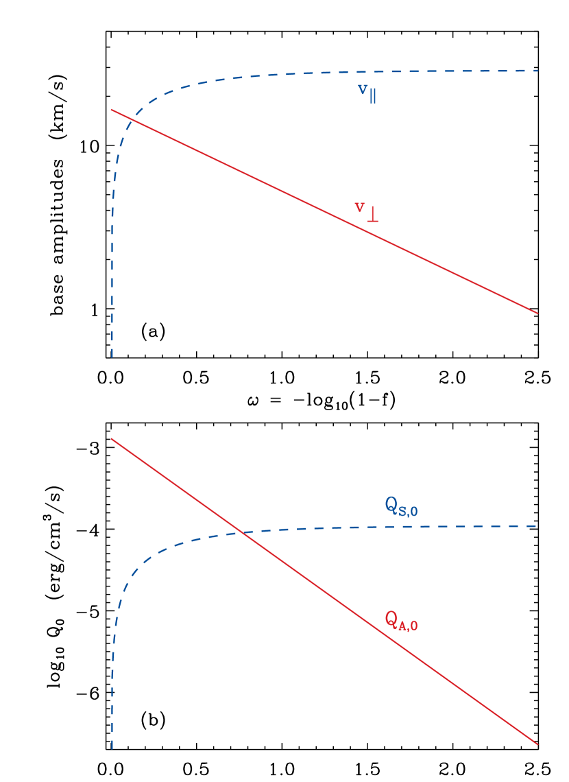
Figure 4 shows how Alfvén waves dominate at low values of $\omega$ and compressive waves dominate at high values. These models assumed $U_{\rm tot}=0.1$ erg cm^-3, $T_{0}=10^{4}$ K, and $P_{0}=0.05$ dyn cm^-2. For these representative parameters, the velocities at the TR are of order 20–30 km/s, which is representative of observational results from nonthermal line broadening (e.g., Banerjee et al., 2011; Hahn & Savin, 2014). Note that $U_{\rm A,0}=U_{\rm S,0}$ when $f=0.5$. However, for the parameters assumed here, the heating rates $Q_{\rm A,0}$ and $Q_{\rm S,0}$ do not become equal until $f=0.83$. In other words, for low values of $f$ it is possible for $Q_{\rm A,0}\gg Q_{\rm S,0}$ even when the velocity amplitudes are comparable to one another.

5. Numerical Methods

We developed a new set of computational tools to solve for the time-steady properties of coronal loops. The Python language was chosen for its well-tested algorithms (e.g., numerical quadrature and the solution of ordinary differential equations), and for its overall flexibility. Below we describe the loop boundary conditions (Section 5.1), the adopted solution procedure (Section 5.2), and the stability of the solutions (Section 5.3).

5.1. Boundary Conditions

At the coronal base ($s=0$), we specify the boundary conditions on the gas pressure ($P_{0}$) and temperature ($T_{0}$). We fix $T_{0}=10^{4}$ K and allow $P_{0}$ to vary as an output of our method (see below). In order to determine additional boundary conditions, we find it convenient to introduce the quantity

$$\Psi\,=\,A\,\kappa(T)\,\frac{dT}{ds}\,\,.$$ (22)

At the apex of the loop ($s=L/2$), we take advantage of the assumed symmetry as shown in Figure 1 and assume

$$\left.\frac{dT}{ds}\right|_{s=L/2}\,=\,\left.\frac{d\Psi}{ds}\right|_{s=L/2}\,=\,0\,\,.$$ (23)

Determining the bottom boundary condition on the temperature gradient $dT/ds$ (i.e., on the quantity $\Psi$) requires slightly more care than just choosing a representative value. This quantity depends sensitively on the modeled thermal energy balance at $T_{0}$. Following Hammer (1982) and Schrijver & van Ballegooijen (2005), we assume that in the upper chromosphere the local heating term $Q_{\rm heat}$ is relatively unimportant in comparison to the conduction and radiative cooling terms. We also simplify the equations in the vicinity of the transition region by using a generalized power-law form of the radiative loss function,

$$\Lambda(T)\,=\,\Lambda_{0}T^{\gamma}\,\,,$$ (24)

for constant values of $\Lambda_{0}$ and $\gamma$. We also use a simpler version of the conductive flux,

$$F\,=\,-\kappa_{0}T^{5/2}\frac{dT}{dz}$$ (25)

that includes only the electron conductivity. The thermal balance equation therefore becomes

$$\frac{dF}{dz}\,=\,-n_{e}^{2}\,\Lambda_{0}T^{\gamma}\,\,.$$ (26)

Multiplying both sides of Equation (26) by $F$, then dividing by $dT/dz$, gives a straightforwardly integrable form

$$F\,dF\,=\,\psi\,T^{\gamma+(1/2)}\,dT$$ (27)

where we assume that $\psi=\kappa_{0}\Lambda_{0}(n_{e}T)^{2}$, proportional to the pressure squared, is a constant across the chromosphere and TR. Integrating both sides yields

$$\frac{1}{2}\,\left(F_{2}^{2}-F_{1}^{2}\right)\,=\,\frac{2\psi}{2\gamma+3}\left[T_{2}^{\gamma+(3/2)}-T_{1}^{\gamma+(3/2)}\right]\,\,,$$ (28)

which can be simplified further by considering that $T$ and $|F|$ are both increasing rapidly with increasing height, such that $T_{2}\gg T_{1}$ and $|F_{2}|\gg|F_{1}|$. This allows us to eliminate the “2” subscript and write

$$F^{2}\,=\,\frac{4\psi\,T^{\gamma+(3/2)}}{2\gamma+3}\,\,.$$ (29)

Using the above definitions, this gives

$$\frac{dT}{dz}\,=\,\sqrt{\left(\frac{4}{2\gamma+3}\right)\,\frac{|Q_{\rm rad}|\,T}{\kappa}}\,\,,$$ (30)

and we calculate $\gamma=9.9$ from our tabulated values of the radiative loss function at $T_{0}=10^{4}$ K. We use this value in Equations (22) and (30) to obtain $\Psi_{0}$ at the lower boundary.

5.2. Solving for Time-Steady Coronal Properties

We solve for the density and temperature throughout the loop using a similar iterative method as Schrijver & van Ballegooijen (2005). Thermal energy conservation is a second-order differential equation, which we separated into two first-order coupled equations: Equation (22) and

$$\frac{d\Psi}{ds}\,=\,-A\,\left(Q_{\rm rad}+Q_{\rm heat}\right)\,\,.$$ (31)

These coupled equations were integrated from the base ($s=0$) to the apex ($s=L/2$) using first-order Euler steps to obtain $T(s)$ and $\Psi(s)$. However, both $Q_{\rm rad}$ and $Q_{\rm heat}$ depend on the coronal density as well as on temperature. To obtain $\rho(s)$, we first integrated Equation (8) for $P(s)$ and also used Equation (4). Doing this requires an initial guess for the temperature. This was given by an analytic solution to a balance between a constant coronal heating rate $Q_{\rm heat}$ and a conduction rate $Q_{\rm cond}$ dominated by the $\kappa_{0}$ electron term. In Cartesian geometry ($A=\mbox{constant}$), this is given by

$$T_{\rm guess}(s)\,=\,(T_{\rm max}-T_{0})\,\left[1-\left(\frac{z}{z_{\rm max}}-1\right)^{2}\right]^{2/7}+\,T_{0}\,\,.$$ (32)

For this first guess, we assumed representative chromospheric and coronal values $T_{0}=10^{4}$ K and $T_{\rm max}=10^{6}$ K.

After creating the above initial temperature function, we also chose an initial guess for $P_{0}$ and proceeded to integrate Equations (22)–(31). In general this initial solution does not satisfy the upper boundary conditions at the loop apex (see above), so we used a Newton-Raphson root finding algorithm to adjust $P_{0}$ toward a value at which Equation (23) is satisfied. We used a fixed initial guess of $P_{0}=0.01$ dyn cm^-2 for the Newton-Raphson method. This value is noticeably lower than the typical base pressure found for the loops, but we find that values of the base pressure that are too high tend to cause divergent solutions. In rare cases when the Newton-Raphson method failed to converge to a solution, we found the root with a more stable but significantly slower bisection method (searching between bounding values of $P_{0}=0.001$ and 10 dyn cm^-2).

As the numerical iteration progresses, the tabulated solutions for $T(s)$ and $P(s)$ are updated and the most recent values are used as guesses in successive rounds of integrating Equations (8) and (22)–(31). The finite-difference tables contain 1000 values of $s$ between the base and apex, and they use a nonuniform grid determined by the function

$$s\,=\,\frac{L}{2}\,\left(\frac{n}{999}\right)^{4}$$ (33)

for $0\leq n\leq 999$. Grid zones are made intentionally dense near $s=0$ in order to capture the rapid temperature changes seen near the base of the loop. We tested the adequacy of these discrete grid parameters (and the use of first-order Euler integration) everywhere in the interior of the loop grid by considering the sum of the three heating/cooling terms in Equation (9) divided by the absolute value of the largest of $Q_{\rm heat}$, $Q_{\rm rad}$, or $Q_{\rm cond}$. When averaged over the length of the loop, this testing ratio was found to almost never exceed 1% for both short and long loops, with the average usually closer to 0.6-0.9% for both cases. At worst, for some combinations of parameters this ratio would reach 15% at some point along the short loops and 27% at some point along the long loops. The instances with the relatively high test ratio tended to coincide with low-$\omega$ and high-$U_{\textrm{tot}}$ loops that would have unrealistically high peak temperatures and temperature gradients near the top of a quiescent corona. The usual low values of the test ratio, especially for loops matching the observational data, indicates a comparable level of fractional accuracy in the other parameters.

Because of the possibility of large relative changes from one iteration to the next, we used an undercorrection scheme for the temperature. This technique was adopted from the ZEPHYR code (Cranmer et al., 2007), and the value at each distance $s$ is updated using

$$T(s)\,=\,T_{\rm old}(s)^{N}\,T_{\rm new}(s)^{1-N}$$ (34)

where $T_{\rm old}$ is the previous iteration’s solution and $T_{\rm new}$ is the direct output of the numerical integration for the current iteration. The constant $N$ is a parameter between 0 and 1 that we set to 0.65 for most cases. For loops that tend to diverge during early iterations, $N$ is first set to 0.2 and then gradually raised to 0.5. Once $T(s)$ is updated, the table of $P(s)$ values is updated, and the process is repeated until the relative temperature difference between one iteration and the next is less than a thousandth of a percent for ten sample grid points spaced evenly through the grid, from $n\,=\,99$ to $n\,=\,999.$

5.3. Stability Considerations

In order to determine whether the time-steady solutions are stable to small perturbations, we test for unstable gravitational stratification. According to Aschwanden et al. (2001), a hydrostatic loop becomes dynamically unstable if

$$\frac{\partial\rho}{\partial s}>0$$ (35)

in the region $0\leq s\leq(L/2)$. Often, it is not necessary to apply this criterion because unstable solutions tend to be unphysical in other ways. In almost all cases, our models exhibit monotonically decreasing density with increasing $s$. If the coronal heating is concentrated too strongly at the base, Equation (35) may end up being satisfied, but these models tend to have insufficient heating toward the apex to maintain a time-steady hot corona. The iteration process in this case leads to negative temperatures, clearly indicating an unphysical solution.

There have been a number of different thermal instabilities proposed that could disrupt some coronal loops and give rise to prominence condensation or “coronal rain” (e.g., Priest, 1978; Habbal & Rosner, 1979; Gómez et al., 1990; Cally & Robb, 1991; Mok et al., 2008; Sasso et al., 2012, 2015; Antolin et al., 2015). This process—in which the loop is stretched or twisted beyond a stable length and cools catastrophically to chromospheric temperatures—is just one of several proposed to explain the highly dynamic and intermittent ultraviolet and X-ray emission seen from loops. However, we defer the study of these kinds of instabilities to future work, since the large-scale quiescent loops modeled in this paper appear to have parameters quite distinct from the (mainly low-lying) unstable loops in the studies cited above.

6. Results

6.1. Model Grids

We consider loops of two different lengths, both given in Table 1, and we refer to them as “long” and “short” loops with reference to the categories defined by Nuevo et al. (2013). The short loops are characterized by $\theta=8\arcdeg$ and $L=0.333\,R_{\odot}$, and the long loops have $\theta=25\arcdeg$ and $L=1.584\,R_{\odot}$. To span the full parameter space of possible loop solutions for each length, we fill a three-dimensional grid of values for $f$, $U_{\rm tot}$, and $L_{\rm damp}$. Twenty different values for $f$ are used, with ten values evenly spaced between 0 and 0.9 (i.e., $0\leq\omega\leq 1$) and another ten values evenly spaced in $\omega$ between 1.3 and 4.0. Ten different values are used for $U_{\rm tot}$ that are evenly spaced on a logarithmic scale bounded by 0.01 and 3.16 erg cm^-3. For most values of $f$ we use 13 different values of $L_{\rm damp}$. However, when $f=0$, the compressive heating term described in Equation (20) vanishes and the coronal heating term is purely Alfvénic. It is therefore only necessary to simulate the loops once for each value of $U_{\rm tot}$ when $f=0$ since the damping length no longer affects the heating rate. For all other values of $f$, the 13 values of $L_{\rm damp}$ are evenly spaced between 0.004 and 0.04 $R_{\odot}$. In total, 4960 loops are simulated, half of which are short and half of which are long.

In order to draw as close a parallel as possible to the findings of Nuevo et al. (2013), we often average values along the loop “legs” at the heights probed by the DEMT technique. The legs are defined to span heights between 0.03 and 0.2 $R_{\odot}$, with the larger value replaced by $z_{\rm max}$ for the short loops that do not extend as high as 0.2 $R_{\odot}$. Specifically, we compute mean temperatures $\langle T\rangle$ in the legs, and we use the slope of a linear fit to $T(z)$ in the legs to determine a mean temperature derivative $\langle dT/dz\rangle$. Models with a positive slope are characterized as “up loops” and those with a negative slope are “down loops.” We note, however, that this one parameter does not always accurately characterize the full spatial dependence of $T(s)$.

6.2. Representative Solutions

Figure 5 shows a selection of temperature and pressure profiles for long loops ($L=1.583\,R_{\odot}$) with a range of $\omega$ values and fixed values of $U_{\rm tot}=1$ erg cm^-3 and $L_{\rm damp}=0.025\,R_{\odot}$. Increasing the amount of mode conversion (i.e., larger values of $\omega$) decreases the total amount of heat deposited along the loop, but it also makes the heating rate more strongly peaked at the footpoints. Aschwanden & Schrijver (2002) showed that a sufficiently steep decrease in $Q(s)$ indeed gives rise to a “down loop” with a local minimum in temperature at the apex.

Figure 5.— Spatial dependence of (a) temperature, (b) gas pressure, and (c) total volumetric heating rate, as a function of distance $s$ traced along long loops. Fixed values of $U_{\rm tot}=1$ erg cm^-3 and $L_{\rm damp}=0.025\,R_{\odot}$ were used with a range of choices for $\omega$ (i.e., mode conversion fraction $f$); see curve labels in panel (a). Up and down loops are plotted in red and blue, respectively.

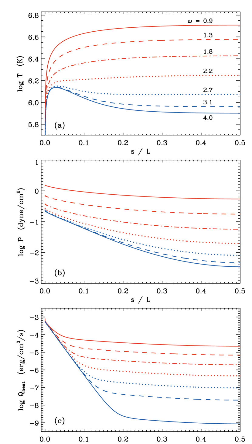
We determined that stable down loops become possible when the mode conversion from Alfvénic to compressive waves is strong (i.e., $\omega\gtrsim 2$). Down loops tend to be seen only for a finite range of $U_{\rm tot}$ values, and the bounds of this range vary inversely with $L_{\rm damp}$. For values of $U_{\rm tot}$ smaller than this finite range, loops remain “normal” (i.e., with monotonically increasing temperatures) for all values of $\omega$. For values of $U_{\rm tot}$ larger than this finite range, the amount of deposited energy at the base appears to be too large for stable coronal loops to exist, and the code is unable to find solutions with $T>0$ everywhere. Detailed maps of the parameter space are shown below.

A number of loops are poorly described as “up” or “down” when their slope $\langle dT/dz\rangle$ is only taken from a linear fit along the legs as described above. In some cases, the peak temperature occurs below the apex, but it is too high for it to be registered as a down loop. Of the 1940 short loops recorded as “up” loops, 214 (11%) have maximum temperatures before the apex, while the same is true for 189 (8.9%) of the 2115 long “up” loops. It is possible that these kinds of loops are not reported by Nuevo et al. (2013) because they only considered loops for which it was possible to create a high-quality linear fit (i.e., with $R^{2}>0.5$) from the DEMT data.

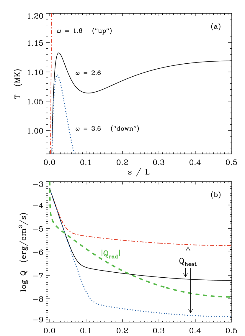
In Figure 6 we also illustrate a transitional nonmonotonic temperature profile that occurs for some long-loop models. Standard up and down loops exhibit one and two temperature maxima (when measured from footpoint to footpoint), respectively. However, these “hybrid” loops exhibit three temperature peaks; i.e., they have a local maximum at the apex, local minima below the apex, and additional local maxima below them on either side. Figure 6(b) illustrates how these hybrid loop cases can occur. Equation (31) indicates that if $|Q_{\rm rad}|>Q_{\rm heat}$, the second derivative of $T$ is positive and the temperature curve near the peak is concave up, consistent with down loops. If $|Q_{\rm rad}|<Q_{\rm heat}$, the curve is concave down at the apex, consistent with up loops. However, in Figure 6(b) we see that for the hybrid loop case, the ratio $|Q_{\rm rad}|/Q_{\rm heat}$ oscillates above and below 1 a number of times between the base and the apex. Thus, despite the strong conduction that tends to smear out small-scale thermal fluctuations along the field, these rare cases do demand multiple minima and maxima in the time-steady $T(s)$.

Figure 6.— Spatial dependence of (a) temperature, and (b) heating/cooling terms in Equation (9), for a set of long loop models with $U_{\rm tot}=0.6$ erg cm^-3, $L_{\rm damp}=0.016\,R_{\odot}$, and a range of values for $\omega$ (see curve labels in panel a). Red, black, and blue curves in panel (b) show $Q_{\rm heat}$, and the green dashed curve shows $|Q_{\rm rad}|$ for only the middle case of $\omega=2.6$.

6.3. Statistical Trends

Figures 7 and 8 are contour plots that indicate the mean temperature gradient $\langle dT/dz\rangle$ in units of MK $R_{\odot}^{-1}$. Each panel plots $\langle dT/dz\rangle$ versus $\omega$ and $U_{\rm tot}$ for a fixed value of $L_{\rm damp}$. Figure 7 shows results for the short loop models, and Figure 8 shows results for the long loop models. We continue the color scheme from Figures 5 and 6 (and from Nuevo et al., 2013) in which up-loop parameters are in red and down-loop parameters are in blue.

Figure 7.— Contour plots of $\langle dT/dz\rangle$ versus $\omega$ and $U_{\rm tot}$, for short-loop models with $L=0.335\,R_{\odot}$. Each panel shows results for a fixed value of $L_{\rm damp}$. Color scales for positive (red) and negative (blue) values of $\langle dT/dz\rangle$ are unique for each panel, and the numbers in color bars are given in units of MK $R_{\odot}^{-1}$. White regions denote parameters with no stable solutions.

Figure 8.— Same as Figure 7, but for the long-loop models with $L=1.583\,R_{\odot}$.

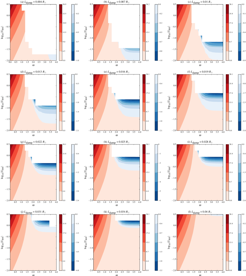
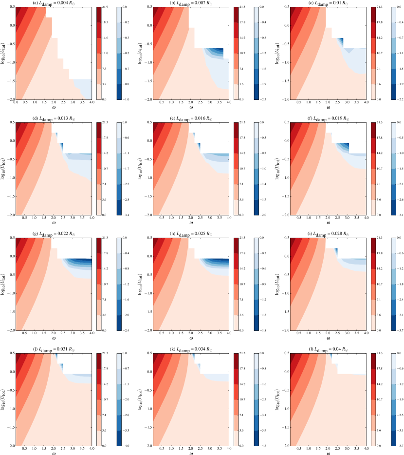
White areas in Figures 7 and 8 indicate combinations of parameters for which the code did not find physically realistic solutions. This tends to occur for the largest values of both $\omega$ and $U_{\rm tot}$; i.e., very strong basal heating and a rapid drop-off of $Q_{\rm heat}$ with increasing height. All cases of “good” solutions (not in white) were found to be also gravitationally stable ($\partial\rho/\partial s<0$) everywhere from footpoint to apex. This result disagrees somewhat with Aschwanden & Schrijver (2002), who found some cases of gravitationally unstable loops with positive temperatures at all values of $s$. These cases occurred for similar (i.e., rapidly decreasing) heating functions as our no-solution cases, but it should be noted that the exponential form for $Q_{\rm heat}(s)$ used by Aschwanden & Schrijver (2002) was different from what is used here.

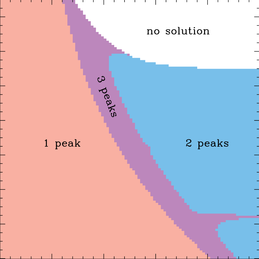
As noted above, the sign of the observationally motivated mean gradient $\langle dT/dz\rangle$ does not always convey an accurate picture of the number of temperature minima and maxima. Specifically, it does not reveal the region of parameter space that produces “hybrid loops” (i.e., ones with three maxima in $T(s)$ from footpoint to footpoint) at all. Thus, in Figure 9 we give an example of the same parameter space shown in Figures 7–8, but with a finer grid and a color scale that denotes the exact topological nature of each model’s temperature profile. This grid contained 12,000 models that were only simulated until the peak temperature had sufficiently converged: 100 values of $\omega$ and 120 values of $U_{\rm tot}$ that span the limits shown in Figure 9. The hybrid loops (3 peaks) occupy a narrow strip of parameter space between the standard regions of up loops (1 peak) and down loops (2 peaks), with some small-scale boundary structure that depends on the relative magnitudes of the heating terms $Q_{\rm rad}$ and $Q_{\rm heat}$ as discussed above. The purple “spurs” that extend to the right in Figure 9 correspond to loops with extremely shallow minima beneath their apex. In those cases the temperature variation at the top of the loop is almost flat, and a plot of $T(s)$ would look nearly indistinguishable from a two-peak down loop.

Figure 9.— Contour plots of the number of maxima in $T(s)$ measured from footpoint to footpoint: with regions of one (red), two (blue), and three (purple) shown alongside the region of no physical solutions (white). Models were computed for the long-loop case, with $L_{\rm damp}=0.034\,R_{\odot}$.

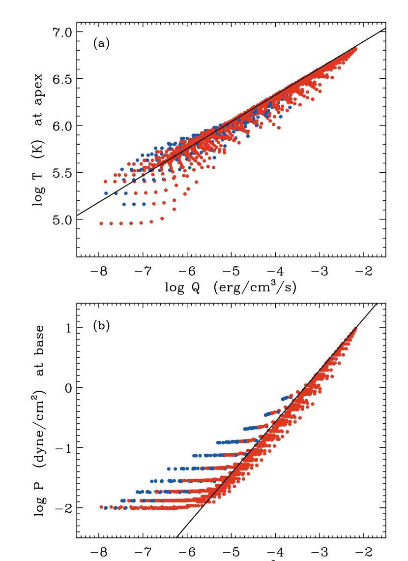
The numerical results for apex temperature $T_{\rm max}$ and base pressure $P_{0}$ can be compared straightforwardly to several existing analytical models (e.g., Rosner et al., 1978; Serio et al., 1981; Aschwanden & Schrijver, 2002; Martens, 2010). For simplicity’s sake we compare only with Rosner et al. (1978, hereafter RTV), who assumed a constant heating rate $Q$ versus distance along a loop with constant pressure and cross section. For standard choices of the radiative and conductive constants, the RTV laws can be written as

$$T_{\rm max}\,=\,1.302\,\,\mbox{MK}\,\left(\frac{Q}{\mbox{10${}^{-4}$ erg cm${}^{-3}$ s${}^{-1}$}}\right)^{2/7}$$

$$\times\left(\frac{L}{\mbox{100 Mm}}\right)^{4/7}$$ (36)

$$P_{0}\,=\,0.1467\,\,\mbox{dyn cm${}^{-2}$}\,\\ \left(\frac{Q}{\mbox{10${}^{-4}$ erg cm${}^{-3}$ s${}^{-1}$}}\right)^{6/7}$$

$$\times\left(\frac{L}{\mbox{100 Mm}}\right)^{5/7}\,\,.$$ (37)

Because the heating rates used in this paper are monotonically decreasing from footpoint to apex, it is not clear what value(s) of $Q$ to use in Equations (36)–(37). After some experimentation, we found that using the geometric mean of the basal and apex heating rates (i.e., the square root of their product) produces reasonable agreement with the RTV predictions. Figure 10 shows a model-by-model comparison for the grid of short loops. A comparable plot for the long loops looks similar to this one, but with all values of $T_{\rm max}$ and $P_{0}$ shifted slightly upwards. Note that the up loops (red points) tend to be more RTV-like than the down loops (blue), since the latter often have a more pronounced and complicated $s$-dependence to their heating rates and pressures.

Figure 10.— Numerically computed apex temperature $T_{\rm max}$ and base pressure $P_{0}$ for short up loops (red points) and short down loops (blue points), plotted against mean heating rate $Q$ (see text). RTV power-law predictions are shown with solid black lines.

For a more direct comparison with the observational data, Figure 11(a) shows how $\langle T\rangle$ and $\langle dT/dz\rangle$ compare against one another. Polygonal outlines (adapted from Figure 10 of Nuevo et al., 2013) give an approximate indication of the observed region of parameter space for up and down loops. Out of the 4960 cases simulated in the short and long loop grids, only 698 of them (14%) fall inside the polygonal outlines. Figure 11(b) outlines the regions of parameter space (in $U_{\rm tot}$ and $\omega$) corresponding to the these models. There seems to be an intermediate range of values for $U_{\rm tot}$ (which changes slightly based on the mode coupling efficiency) required to match the observations. More wave power would result in too much heating (i.e., $\langle T\rangle>2$ MK), and less wave power would give too little ($\langle T\rangle<0.8$ MK). There are no clear limiting values of $L_{\rm damp}$ that identify the subset of models that agree with the observations.

Figure 11.— (a) Scatter plot of fitted mean loop temperatures $\langle T\rangle$ versus the mean temperature gradient $\langle dT/dz\rangle$. Up-loop solutions are shown for short loops (orange circles) and long loops (dark red X’s). Down-loop solutions are shown for short loops (cyan circles) and long loops (dark blue X’s). Outside the observed region of parameter space (Nuevo et al., 2013), symbols are black. (b) Regions of model parameter space (as in Figures 7–9) that correspond approximately to the models inside the observed regions in panel (a). Up-loop regions are in red and down-loop regions are in blue.

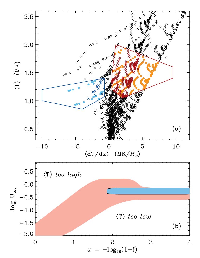
Figure 11 gives the general impression that the measured quiescent up loops are produced when there is a small amount of mode energy transfer from Alfvén to compressive waves at the TR, and the down loops are produced when there is large mode energy transfer. For low values of $\omega$, the band of observationally appropriate parameters for up loops corresponds to basal values of the Alfvén velocity amplitude around 3–6 km s^-1. These values are quite a bit smaller than the canonical 20–30 km s^-1 nonthermal amplitudes often seen in the brighter and more compact active-region loops. However, the large quiescent loops traced out by the DEMT technique (Huang et al., 2012; Nuevo et al., 2013) are believed to comprise a diffuse coronal background that must be heated more weakly than the small and bright loops that are easier to resolve in extreme ultraviolet images.

Nuevo et al. (2013) measured the plasma $\beta$ ratio for the observed loops, where

$$\beta\,=\,\frac{P}{B^{2}/8\pi}\,\,.$$ (38)

The leg-averaged value $\langle\beta\rangle$ was found to be systematically larger for down loops (median values of 1–3) than for up loops (median values of 0.5–0.9). Nuevo et al. (2013) attributed this difference mainly to the fact that down loops tend to have weaker magnetic fields than up loops. They also speculated that the larger values of $\langle\beta\rangle$ in the down loops should make them more susceptible to mode conversion between Alfvén and compressive waves.

Unfortunately, we cannot make a direct comparison with the observed trends in $\beta$ because our modeled loops do not depend on an absolute normalization for $B$. However, we have estimated the value of $\beta_{0}$ at the TR under the assumption that all loops share a common value of $B=2$ G at the TR. In fact, we believe $\beta_{0}$ may be a more important parameter for determining the degree of basal mode conversion than $\langle\beta\rangle$ measured higher up in the corona. With the above assumption about $B$, the up loops within the red polygonal outline in Figure 11(a) have a median value of $\beta_{0}=0.636$, and the corresponding down loops have a median value of $\beta_{0}=1.32$. This difference is attributable solely to differences in $P_{0}$ in the two populations of models, but it does go in the same direction as the observed variation in $\langle\beta\rangle$. It should be noted that a similar trend in base pressures is also evident in the measured mean values given in Table 1 of Nuevo et al. (2013). Thus, it is unclear whether the observed differences in $\langle\beta\rangle$ between the up and down loops can be attributed primarily to differences in gas pressure or magnetic pressure.

7. Discussion and Conclusions

One key goal of this paper was to test the conjecture made by Nuevo et al. (2013) that mode conversion at the TR—from Alfvénic to compressive waves—can be responsible for the existence of coronal loops with an “inverted” temperature structure. We constructed a large grid of models with two sources of time-steady coronal heating: a turbulent cascade of incompressible Alfvén waves (which generally produces heating that varies slowly with height) and the rapid basal dissipation of compressive waves (whose heating is highly peaked at the loop footpoints). The production of stable loops with radially decreasing temperatures requires nearly all (i.e., $>$99%) of the Alfvén wave energy to be converted to compressive waves that deposit their heat at the base. This was anticipated in earlier parameter studies (Serio et al., 1981; Aschwanden & Schrijver, 2002), but we have quantified how much wave-mode energy transfer is needed to produce such highly peaked heating functions.

One aspect of the models that was relegated to free-parameter status was the damping length $L_{\rm damp}$ of the compressive waves. Our grid of models assumed values of $L_{\rm damp}$ that vary over an order of magnitude between 0.004 and 0.04 $R_{\odot}$. It is worthwhile to compare these values with predictions from the theory of magnetoacoustic wave dissipation. Cranmer et al. (2007) modeled this by assuming two sources of energy loss: (linear) thermal conductivity and (nonlinear) shock entropy evolution. The latter was found to be more important in the chromosphere, and the former was found to be more important in the corona. Thus, we examine heat conductivity, which has an effective damping length $\tilde{L}_{\rm damp}=c_{s}/2\gamma_{c}$, where $\gamma_{c}$ is the linear damping rate due to electron heat conduction. Making use of classical expressions for this transport coefficient (see also Hung & Barnes, 1973; Whang, 1997),

$$\tilde{L}_{\rm damp}\,\approx\,0.0133\,R_{\odot}\,\left(\frac{\rho}{10^{-16}\,\mbox{g cm${}^{-3}$}}\right)$$

$$\times\left(\frac{T}{10^{5}\,\mbox{K}}\right)^{-1}\left(\frac{\Pi}{\mbox{5 min}}\right)^{2}$$ (39)

where $\Pi$ is the acoustic wave period. When evaluated at the chromospheric base, this damping length is very large (10–100 $R_{\odot}$), but it drops rapidly with increasing height. For typical coronal-loop apex properties, this theoretical $\tilde{L}_{\rm damp}$ is of order $10^{-3}\,R_{\odot}$. The height at which the value of $\tilde{L}_{\rm damp}$ matters most to the models (Equations (19)–(20)) is essentially $s\approx\tilde{L}_{\rm damp}$. This is the distance above the TR at which the damping finally gets a chance to reduce the wave energy density by a significant amount. Thus, we can identify a unique damping length by finding the location at which $\tilde{L}_{\rm damp}$ (a decreasing function of distance along the loop) and $s$ (an increasing function, by definition) become equal to one another.

For each of the 798 models inside the polygons in Figure 11, we determined a unique conductive damping length $\tilde{L}_{\rm damp}$ using the above procedure. We assumed a fiducial chromospheric value of $\Pi=3$ minutes (Noyes, 1967; Rutten, 2003; Judge, 2006). This produced a range of values that matched the initial assumptions from our grid quite well. The minimum, median, and maximum values of $\tilde{L}_{\rm damp}$ were 0.0052, 0.0072, 0.047 $R_{\odot}$, respectively. If we had used larger periods, such as the 20–30 minute values observed for off-limb intensity oscillations (e.g., Ofman et al., 1999; Liu et al., 2015), then Equation (39) would have given much larger damping lengths. However, such long period waves may be susceptible to conversion to other types of conductivity-dominated modes. Bogdan (2006) showed that such modes can dissipate rapidly at the coronal base, thus effectively reducing $\tilde{L}_{\rm damp}$ despite the large values of $\Pi$.

Although the models presented in this paper have helped to refine the connections between wave mode conversion and loop temperature structure, there are many other improvements that would allow us to build a more comprehensive understanding of heating in the closed corona. For example, instead of assuming the compressive waves are generated impulsively at the lower boundary, the models should include a self-consistent description of the height-dependence of plasma parameters in the chromosphere and TR, as well as the $\beta$-dependent physics of mode conversion (see also Cranmer & Woolsey, 2015). Time-dependent simulations are beginning to show a broad diversity of mode coupling processes in this complex environment (Matsumoto & Suzuki, 2014; Arber et al., 2016). Lastly, our adopted rate of heating due to MHD turbulent cascade was a relatively simple phenomenological scaling law, but there are others (e.g., Rappazzo et al., 2008; van Ballegooijen et al., 2011; Asgari-Targhi et al., 2013; Bourdin et al., 2016) that may be more realistic.

Huang et al. (2012) and Nuevo et al. (2013) found that inverted-temperature loops tend to occur most frequently at low heliographic latitudes, and that they preferentially appear in the “deep” solar minimum. Thus, the footpoint locations of down loops correspond with some of the weakest large-scale magnetic fields seen over the solar cycle. It is not surprising that they may have higher plasma $\beta$ ratios and greater amounts of wave mode conversion than the rest of the corona. Trans-equatorial loops like these connect to the cusp regions of large helmet streamers, which also exhibit $\beta\gtrsim 1$ due to their weak fields (Li et al., 1998; Vásquez et al., 2011). The overall MHD stability of these regions—including their propensity to produce episodic bursts of solar wind (Sheeley et al., 1997; Wang et al., 2000; Suess & Nerney, 2004)—is likely to depend sensitively on the physics of waves and their dissipation as studied here.

References

- Altschuler & Newkirk (1969) Altschuler, M. D., & Newkirk, G. 1969, Sol. Phys., 9, 131
- Antolin et al. (2015) Antolin, P., Vissers, G., Pereira, T. M. D., et al. 2015, ApJ, 806, 81
- Arber et al. (2016) Arber, T. D., Brady, C. S., & Shelyag, S. 2016, ApJ, 817, 94
- Aschwanden (2006) Aschwanden, M. J. 2006, Physics of the Solar Corona: An Introduction with Problems and Solutions, 2nd ed. (Berlin: Springer)
- Aschwanden et al. (2001) Aschwanden, M. J., Schrijver, C. J., & Alexander, D. 2001, ApJ, 550, 1036
- Aschwanden & Schrijver (2002) Aschwanden, M. J., & Schrijver, C. J. 2002, ApJS, 142, 269
- Asgari-Targhi et al. (2013) Asgari-Targhi, M., van Ballegooijen, A. A., Cranmer, S. R., & DeLuca, E. E. 2013, ApJ, 773, 111
- Banerjee et al. (2011) Banerjee, D., Gupta, G. R., & Teriaca, L. 2011, Space Sci. Rev., 158, 267
- Bogdan (2006) Bogdan, T. J. 2006, ApJ, 643, 532
- Bogdan et al. (2002) Bogdan, T. J., Rosenthal, C. S., Carlsson, M., et al. 2002, Astron. Nachr., 323, 196
- Bourdin et al. (2016) Bourdin, P.-A., Bingert, S., & Peter, H. 2016, A&A, 589, A86
- Breech et al. (2008) Breech, B., Matthaeus, W. H., Minnie, J., et al. 2008, J. Geophys. Res., 113, A08105
- Cally & Robb (1991) Cally, P. S., & Robb, T. D. 1991, ApJ, 372, 329
- Cargill & Priest (1980) Cargill, P. J., & Priest, E. R. 1980, Sol. Phys., 65, 251
- Chandran et al. (2011) Chandran, B. D. G., Dennis, T. J., Quataert, E., & Bale, S. D. 2011, ApJ, 743, 197
- Close et al. (2003) Close, R. M., Parnell, C. E., Mackay, D. H., & Priest, E. R. 2003, Sol. Phys., 212, 251
- Craig et al. (1978) Craig, I. J. D., McClymont, A. N., & Underwood, J. H. 1978, A&A, 70, 1
- Cranmer & van Ballegooijen (2012) Cranmer, S. R., & van Ballegooijen, A. A. 2012, ApJ, 754, 92
- Cranmer et al. (2007) Cranmer, S. R., van Ballegooijen, A. A., & Edgar, R. J. 2007, ApJS, 171, 520
- Cranmer & Woolsey (2015) Cranmer, S. R., & Woolsey, L. N. 2015, ApJ, 812, 71
- Dahlburg et al. (2012) Dahlburg, R. B., Einaudi, G., Rappazzo, A. F., & Velli, M. 2012, A&A, 544, L20
- DeRosa et al. (2012) DeRosa, M. L., Brun, A. S., & Hoeksema, J. T. 2012, ApJ, 757, 96
- Dmitruk et al. (2002) Dmitruk, P., Matthaeus, W. H., Milano, L. J., et al. 2002, ApJ, 575, 571
- Fletcher et al. (2015) Fletcher, L., Cargill, P. J., Antiochos, S. K., & Gudiksen, B. V. 2015, Space Sci. Rev.,188, 211
- Fontenla et al. (1990) Fontenla, J. M., Avrett, E. H., & Loeser, R. 1990, ApJ, 355, 700
- Frazin et al. (2005) Frazin, R. A., Kamalabadi, F., & Weber, M. A. 2005, ApJ, 628, 1070
- Frazin et al. (2009) Frazin, R. A., Vásquez, A. M., & Kamalabadi, F. 2009, ApJ, 701, 547
- Gómez et al. (1990) Gómez, D. O., Sicardi Schifino, A., & Ferro Fontán, C. 1990, ApJ, 352, 318
- Gómez et al. (2000) Gómez, D. O., Dmitruk, P. A., & Milano, L. J. 2000, Sol. Phys., 195, 299
- Habbal & Rosner (1979) Habbal, S. R., & Rosner, R. 1979, ApJ, 234, 1113
- Hahn & Savin (2014) Hahn, M., & Savin, D. W. 2014, ApJ, 795, 111
- Hammer (1982) Hammer, R. 1982, ApJ, 259, 767
- Hansteen et al. (2015) Hansteen, V., Guerreiro, N., De Pontieu, B., & Carlsson, M. 2015, ApJ, 811, 106
- Hoeksema & Scherrer (1986) Hoeksema, J. T., & Scherrer, P. H. 1986, Sol. Phys., 105, 205
- Hollweg (1971) Hollweg, J. V. 1971, J. Geophys. Res., 76, 5155
- Hollweg (1986) Hollweg, J. V. 1986, J. Geophys. Res., 91, 4111
- Hossain et al. (1995) Hossain, M., Gray, P. C., Pontius, D. H., Jr., Matthaeus, W. H., & Oughton, S. 1995, Phys. Fluids, 7, 2886
- Howes & Nielson (2013) Howes, G. G., & Nielson, K. D. 2013, Phys. Plasmas, 20, 072302
- Huang et al. (2012) Huang, Z., Frazin, R. A., Landi, E., et al. 2012, ApJ, 755, 86
- Hung & Barnes (1973) Hung, R. J., & Barnes, A. 1973, ApJ, 180, 253
- Iroshnikov (1963) Iroshnikov, P. S. 1963, AZh, 40, 742
- Judge (2006) Judge, P. 2006, in ASP Conf. Proc. 354, Solar MHD Theory and Observations: A High Spatial Resolution Perspective, ed. H. Uitenbroek, J. Leibacher, R. Stein (San Francisco: ASP), 259
- Kaghashvili (2007) Kaghashvili, E. K. 2007, Phys. Plasmas, 14, 044502
- Killie et al. (2005) Killie, M. A., Lie-Svendsen, Ø., & Leer, E. 2005, ApJ, 632, L155
- Kiyani et al. (2015) Kiyani, K. H., Osman, K. T., & Chapman, S. C. 2015, Phil. Trans. Roy. Soc. A, 373, 20140155
- Klimchuk (2015) Klimchuk, J. A. 2015, Phil. Trans. Roy. Soc. A, 373, 20140256
- Kraichnan (1965) Kraichnan, R. H. 1965, Phys. Fluids, 8, 1385
- Krishna Prasad et al. (2012) Krishna Prasad, S., Banerjee, D., Van Doorsselaere, T., & Singh, J. 2012, A&A, 546, A50
- Krishna Prasad et al. (2013) Krishna Prasad, S., Singh, J., & Ichimoto, K. 2013, ApJ, 765, L46
- Laming & Feldman (2003) Laming, J. M., & Feldman, U. 2003, ApJ, 591, 1257
- Lemen et al. (2012) Lemen, J. R., Title, A. M., Akin, D. J., et al. 2012, Sol. Phys., 275, 17
- Li et al. (1998) Li, J., Raymond, J. C., Acton, L. W., et al. 1998, ApJ, 506, 431
- Liu et al. (2015) Liu, J., McIntosh, S. W., De Moortel, I., et al. 2015, ApJ, 806, 273
- Lundquist et al. (2008) Lundquist, L. L., Fisher, G. H., & McTiernan, J. M. 2008, ApJS, 179, 509
- Martens (2010) Martens, P. C. H. 2010, ApJ, 714, 1290
- Matsumoto & Suzuki (2014) Matsumoto, T., & Suzuki, T. K. 2014, MNRAS, 440, 971
- Matthaeus et al. (1999) Matthaeus, W. H., Zank, G. P., Oughton, S., Mullan, D. J., & Dmitruk, P. 1999, ApJ, 523, L93
- Mok et al. (2008) Mok, Y., Mikić, Z., Lionello, R., & Linker, J. A. 2008, ApJ, 679, L161
- Nakariakov et al. (1998) Nakariakov, V. M., Roberts, B., & Murawski, K. 1998, A&A, 332, 795
- Noyes (1967) Noyes, R. W. 1967, in IAU Symp. 28, Aerodynamic Phenomena in Stellar Atmospheres, ed. R. Thomas (London: Academic Press), 293
- Nuevo et al. (2013) Nuevo, F. A., Huang, Z., Frazin, R., et al. 2013, ApJ, 773, 9
- Ofman et al. (1999) Ofman, L., Nakariakov, V. M., & DeForest, C. E. 1999, ApJ, 514, 441
- Orlando et al. (1995) Orlando, S., Peres, G., & Serio, S. 1995, A&A, 294, 861
- Parnell & De Moortel (2012) Parnell, C. E., & De Moortel, I. 2012, Phil. Trans. Roy. Soc. A, 370, 3217
- Priest (1978) Priest, E. R. 1978, Sol. Phys., 58, 57
- Rappazzo et al. (2008) Rappazzo, A. F., Velli, M., Einaudi, G., & Dahlburg, R. B. 2008, ApJ, 677, 1348
- Rosner et al. (1978) Rosner, R., Tucker, W. H., & Vaiana, G. S. 1978, ApJ, 220, 643 (RTV)
- Rutten (2003) Rutten, R. J. 2003, in Turbulence, Waves and Instabilities in the Solar Plasma, ed. R. Erdélyi, K. Petrovay, B. Roberts, M. Aschwanden (Dordrecht: Kluwer), 145
- Sasso et al. (2012) Sasso, C., Andretta, V., Spadaro, D., et al. 2012, A&A, 537, A150
- Sasso et al. (2015) Sasso, C., Andretta, V., & Spadaro, D. 2015, A&A, 583, A54
- Schatten et al. (1969) Schatten, K. H., Wilcox, J. M., & Ness, N. F. 1969, Sol. Phys., 6, 442
- Schrijver & van Ballegooijen (2005) Schrijver, C. J., & van Ballegooijen, A. A. 2005, ApJ, 630, 552
- Serio et al. (1981) Serio, S., Peres, G., Vaiana, G. S., et al. 1981, ApJ, 243, 288
- Sheeley et al. (1997) Sheeley, N. R., Wang, Y.-M., Hawley, S. H., et al. 1997, ApJ, 484, 472
- Spadaro et al. (2003) Spadaro, D., Lanza, A. F., Lanzafame, A. C., et al. 2003, ApJ, 582, 486
- Spitzer (1962) Spitzer, L., Jr. 1962, Physics of Fully Ionized Gases, 2nd ed. (New York: Wiley)
- Steele & Priest (1990) Steele, C. D. C., & Priest, E. R. 1990, Sol. Phys., 125, 295
- Stein & Schwartz (1972) Stein, R. F., & Schwartz, R. A. 1972, ApJ, 177, 807
- Suess & Nerney (2004) Suess, S. T., & Nerney, S. 2004, Adv. Space Res., 33, 668
- Threlfall et al. (2013) Threlfall, J., De Moortel, I., McIntosh, S. W., et al. 2013, A&A, 556, A124
- van Ballegooijen (1986) van Ballegooijen, A. A. 1986, ApJ, 311, 1001
- van Ballegooijen et al. (2014) van Ballegooijen, A. A., Asgari-Targhi, M., & Berger, M. A. 2014, ApJ, 787, 87
- van Ballegooijen et al. (2011) van Ballegooijen, A. A., Asgari-Targhi, M., Cranmer, S. R., & DeLuca, E. 2011, ApJ, 736, 3
- van der Holst et al. (2014) van der Holst, B., Sokolov, I. V., Meng, X., et al. 2014, ApJ, 782, 81
- Vásquez et al. (2010) Vásquez, A. M., Frazin, R. A., & Manchester, W. B. 2010, ApJ, 715, 1352
- Vásquez et al. (2011) Vásquez, A. M., Huang, Z., Manchester, W. B., et al. 2011, Sol. Phys., 274, 259
- Wallenhorst (1982) Wallenhorst, S. G. 1982, Sol. Phys., 79, 333
- Wang (1998) Wang, Y.-M. 1998, ApJ, 501, L145
- Wang et al. (2000) Wang, Y.-M., Sheeley, N. R., Socker, D. G., et al. 2000, J. Geophys. Res., 105, 25133
- Whang (1997) Whang, Y. C. 1997, ApJ, 485, 389
- Zhou & Matthaeus (1990) Zhou, Y., & Matthaeus, W. H. 1990, J. Geophys. Res., 95, 10291