Numerical calculation of the Casimir–Polder interaction between a graphene sheet with vacancies and an atom

Abstract

In this work the Casimir–Polder interaction energy between a rubidium atom and a disordered graphene sheet is investigated beyond the Dirac cone approximation by means of accurate real-space tight-binding calculations. As a model of defected graphene, we consider a tight-binding model of $\pi$-electrons on a honeycomb lattice with a small concentration of vacancies. The optical response of the graphene sheet is evaluated with full spectral resolution by means of exact Chebyshev polynomial expansions of the Kubo formula in large lattices with in excess of ten million atoms. At low temperatures, the optical response of defected graphene is found to display two qualitatively distinct behavior with a clear transition around finite (non-zero) Fermi energy. In the vicinity of the Dirac point, the imaginary part of optical conductivity is negative for low frequencies while the real part is strongly suppressed. On the other hand, for high doping, it has the same features found in the Drude model within the Dirac cone approximation, namely, a Drude peak at small frequencies and a change of sign in the imaginary part above the interband threshold. These characteristics translate into a non-monotonic behavior of the Casimir–Polder interaction energy with very small variation with doping in the vicinity of the neutrality point while having the same form of the interaction calculated with Drude’s model at high electronic density.

I Introduction

Dispersive forces—including van der Waals, Casimir, and Casimir–Polder types—are interactions between neutral, but polarizable objects, and have their origin in fluctuations of the vacuum electromagnetic field reviews . The Casimir force involves interactions between macroscopic objects casimir , such as plates, while Casimir–Polder forces act between a macroscopic object and a microscopic particle casimirpolder . Van der Waals forces act between objects in the short range regime, where effects of retardation can be neglected. These forces are dominant on nano and micro scales and their control and manipulation are important to applications, such as nano-electromechanical systems, among others nem ; nem2 . Dispersive forces are strongly influenced by the shape and material composition, as well as the dielectric and magnetic responses of the objects they act upon. It is possible to tailor the sign and magnitude of dispersive forces by tuning, for example, the dielectric response of the plate. As a result, the correct modeling of dispersive forces from a materials science perspective becomes important LiliaWoods-Review-2015 ; Galina-Review_2009 .

Since its isolation, graphene has attracted great attention, owing to its unconventional low-energy physics described by the Dirac–Weyl equation for massless excitations in two spatial dimensions, and a number of desirable physical properties, including superior mechanical strength, high charge carrier mobilities, and gate-tunable optical response rgraphene1 ; rgraphene2 ; rgraphene3 . Intense theoretical effort has been devoted to the study of Casimir Bordag2009 ; Bordag2012 ; Drosdoff ; Fialkovsky ; Galina2013 ; Gomez ; MacdonaldPRL ; Sernelius ; Svetovoy ; Klimchitskaya-Mostepanenko-14 ; Galina2014 ; Bordag2016 ; Drosdoff2012-2 and Casimir–Polder Churkin ; Galina2014 ; Chaichia3 ; Judd ; Sofia-Scheel-13 ; Cysne_2014 ; LiliaWoods-2016 interactions in graphene and related systems CasimirChern ; abinitio . The Casimir–Polder energy of different atoms on single layer has been considered in Refs. Churkin ; Chaichia3 , and on multilayer graphene in Ref. LiliaWoods-2016 . The tunability of interactions have been demonstrated in atom-on-graphene Cysne_2014 and in graphene bilayers MacdonaldPRL using external magnetic fields, and in a graphene–metal system by tuning the chemical potential Bordag2016 . In general, a Dirac cone approximation is considered where the reflection coefficients of graphene are calculated either within the hydrodynamic model or the polarization tensor with a Drude model approach. The weakness of dispersive interactions on graphene systems is experimentally challenging, and most of theoretical predictions point to an enhancement of interactions by charge doping Drosdoff2012-2 ; Bordag2016 . Recently, the control of the interaction between graphene and naphtalene molecule at short distances (van der Waals regime) has been achieved exploiting the high tunability of the chemical potential Huttman-2015 .

Recent advances in the understanding of dispersive interactions involving graphene and other low-dimensional systems have shown the importance of a detailed characterization the electrical response of the layers for the control and tailoring of dispersive forces. Although ab initio methods have been used to model van der Waals forces abinitio , a more materials oriented approach to study Casimir interactions is still needed. In this article, we consider a realistic model of a large graphene sheet with vacancies. To determine the Fermi energy dependence of its optical conductivity, we employ an accurate large-scale quantum transport approach based on an exact polynomial representation of disordered Green functions recently introduced in Ref. Ferreira15 . The large number of expansion moments in the numerical evaluation of the Kubo formula in large graphene lattices allows us to determine the optical response with fine spectral resolution. This information is then used to compute the Casimir–Polder force between a defected graphene sheet and an atom in function of the charge doping, and compare it with the force calculated using the Drude model. Far from the Dirac point, the Casimir–Polder force varies linearly with the chemical potential. The Drude model is found in accord with numerical calculations in that regime, as expected, but fails to capture the behavior of the Casimir–Polder force close to the Dirac point. Furthermore, we find that the strength of the interaction is reduced in the vicinity of the Dirac point, following the trend of the dc conductivity Ferreira15 , and increases again above a certain Fermi energy scale $\mu^{*}>0$, in contrast with the monotonic enhancement of interactions predicted by calculations based on perfect graphene models.

This article is organized as follows. Section II outlines the real space quantum transport methodology used to extract the optical conductivity of large disordered graphene lattices. In Sec. II.1, we apply the methodology to a graphene lattice with a dilute concentration of vacancies. In section III we describe the calculation of the Casimir–Polder force between the graphene layer and a rubidium atom and present our results. Finally, section IV summarizes the main findings of our work.

II METHODOLOGY

The graphene sheet is modeled by a tight-binding Hamiltonian of $\pi$ electrons defined on a honeycomb lattice

$$\hat{H}=-t\sum_{\langle i,j\rangle}\>(\hat{a}_{i}^{\dagger}\hat{b}_{j}+\textrm{H.c.})\,,$$ (1)

where the operator $a_{i}^{\dagger}$ creates an electron at site $\mathbf{r}_{i}=(x_{i},y_{i})$ on sublattice $A$ (an equivalent definition holds for sublattice $B$), and $t=2.7$ eV is the nearest-neighbor hopping integral RMPgraphene . The point defects are introduced by removing sites in any sublattice at random (compensated vacancies). The defect concentration is $n_{i}=N_{d}/D$, where $N_{d}$ is the number of missing carbon atoms and $D$ is the number of sites in the pristine lattice (see Fig. 1).

The real part of the diagonal optical conductivity at zero temperature and finite frequency is given by Mahan

$$\Re\,\sigma(\omega)=\frac{\pi}{\omega\,\Omega}\int_{\mu-\hbar\omega}^{\mu}d\epsilon\,\,\textrm{Tr}\,\langle\hat{J}_{x}\,\hat{A}(\epsilon)\,\hat{J}_{x}\,\hat{A}(\epsilon+\hbar\omega)\rangle_{\textrm{c}}\,,$$ (2)

where $\hat{J}_{x}=(ite/\hbar)\sum_{\langle i,j\rangle}(x_{i}-x_{j})(\hat{a}_{i}^{\dagger}\hat{b}_{j}-\textrm{H.c.})$ is the $x$-component of the current density operator, and

$$\hat{A}(\epsilon)=-\frac{1}{\pi}\,\Im\,\frac{1}{\epsilon-\hat{H}+i\eta}\,,$$ (3)

is the spectral operator of the system. The symbol $\langle...\rangle_{\textrm{c}}$ denotes configurational average, $\Omega$ is the area of the lattice, $\mu$ is the chemical potential, and $\eta$ is a small broadening parameter required for numerical convergence. Physically, the broadening $\eta=\hbar/\tau_{i}$ mimics the effect of uncorrelated inelastic scattering processes with lifetime $\tau_{i}$ (e.g., due to phonons), and can be viewed as an energy uncertainty due to coupling of electrons to a bath Thouless_81 ; Imry .

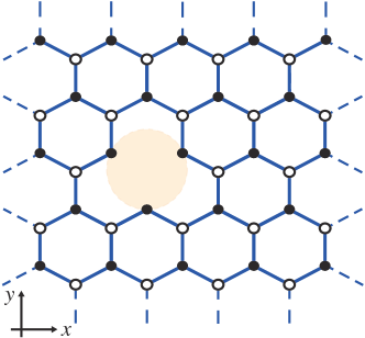
Figure 1: Schematic of a graphene lattice with vacancy defects. $A$($B$) sublattices are represented by filled (open) circles. Shaded area shows a vacancy. The numerical simulations in this work have a computational domain of size $3200\times 3200$, with periodic boundary conditions on both directions (torus).

The response functions of large tight-binding systems can be assessed numerically by means of specialized spectral methods spectral_Kosloff84 ; spectral_Roche_Mayou_97 ; spectral_Tanaka98 ; spectral_Weisse04 ; spectral_Yuan10 ; spectral_Holzner11 . A particularly convenient approach is the kernel polynomial method KPM , in which spectral operators are approximated by accurate matrix polynomial expansions. The coefficients of the polynomial expansion are computed recursively thereby bypassing matrix inversion that limits systems sizes in exact diagonalization schemes. The kernel polynomial method has been applied intensively to study the electronic properties of disordered graphene KPM_G_Ferreira11 ; KPM_G_Fan14 ; KPM_G_Garcia15 ; ReviewChebG . Here, we make use of an exact Chebyshev polynomial representation of the resolvent operator recently obtained in Ref. Ferreira15 , in order to perform numerically exact large-scale calculations of the optical conductivity. The starting point in our approach is the operator identity $(z-\hat{h})^{-1}=\sum_{n=0}^{\infty}a_{n}(z)\,\mathcal{T}_{n}(\hat{h})\,,$ where $z=(\epsilon+i\eta)/W$, $\hat{h}$ is the rescaled Hamiltonian of disordered graphene $\hat{h}=\hat{H}/W$ (here $W=3t$ is half bandwidth), and $\mathcal{T}_{n}(\hat{h})$ are matrix Chebyshev polynomials of first kind (see Appendix). Using this expansion, the spectral operator [Eq. (3)] can be recast into the form

$$\hat{A}=-\frac{1}{\pi W}\sum_{n=0}^{\infty}\Im[a_{n}(z)]\,\mathcal{T}_{n}(\hat{h})\,,$$ (4)

whose action on a given basis set can be computed iteratively by standard Chebyshev recursion KPM .

In a numerical implementation, the sum in Eq. (4) is truncated when convergence to a given desired accuracy is achieved. The $N$th-order approximation to the optical conductivity is therefore given by

$$\Re\>\sigma^{(N)}(\omega)=\frac{\pi}{\,\omega\,\Omega}\sum_{n,m=0}^{N-1}\sigma_{nm}\,A_{nm}(\mu,\omega)\,,$$ (5)

where

$$\sigma_{nm} =\textrm{Tr}\>\langle\hat{J}_{x}\,\mathcal{T}_{n}(\hat{h})\,\hat{J}_{x}\,\mathcal{T}_{m}(\hat{h})\rangle_{\textrm{c}}\,,$$ (6)

$$A_{nm}(\mu,\omega) =\frac{1}{\pi^{2}W^{2}}\int_{\mu-\hbar\omega}^{\mu}d\epsilon\,\alpha_{n}(\epsilon)\alpha_{m}(\epsilon+\hbar\omega)\,,$$ (7)

and $\alpha_{n}(\epsilon)$ is a shorthand for $\Im[a_{n}\left((\epsilon+i\eta)/W\right)]$. Clearly, the problem boils down to the evaluation of $\sigma_{nm}$, which contains the relevant dynamical information. Once the expansion moments have been determined, the optical conductivity can be quickly retrieved using Eq. (5). For a recent review on the application of Chebyshev expansions in the context of disordered graphene, we refer the reader to Ref. ReviewChebG .

II.1 Optical Conductivity of Disordered Graphene

With the approach described in the previous section we can study, in a numerically rigorous way, the optical conductivity of graphene in the presence of strong disorder—for instance, that created by vacancies, or strongly adsorbed atoms for the same purpose KPM_G_Ferreira11 .

As a model system of disordered graphene, we have simulated a large lattice of size $3200\times 3200$ (atoms) with a dilute vacancy concentration, $n_{i}=0.4$% (atomic ratio). The spectrum of graphene with vacancies is particle-hole symmetric, and hence for simplicity we assume $\mu\geq 0$ in what follows. Owing to the large system size, it suffices to consider a single disorder realization when performing configurational averages. The optical conductivity for a typical broadening parameter is shown in Fig. 2. To ensure convergence of the optical conductivity to a good precision [Eq. (5)], we have computed a very large number of Chebyshev iterations $N^{2}=8000^{2}$. Finally, the trace in Eq. (6) has been performed by means of stochastic trace evaluation (STE) technique KPM . We have used 5000 random vectors in the STE to enable determination of $\sigma_{nm}$ with accuracy better than $1\%$.

Roughly speaking, we expect that disorder should play a role at low frequencies, $\hbar\omega\ll\mu$. This is the case if the Fermi energy is not too small. Indeed, we see in Fig. 2 that for a Fermi energy of 0.5 eV there is a well defined step at twice the Fermi energy.

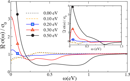
Figure 2: The optical conductivity of graphene with a dilute vacancy concentration $n_{i}=0.4\%$ at selected values of the chemical potential $\mu$ with $\eta\approx 8$ meV.

A calculation of the optical conductivity based on the Boltzmann equation, given by

$$\sigma_{\textrm{D}}(\omega,T,\mu)=\sigma_{\textrm{D},0}(T,\mu)\frac{1}{1-i\omega\tau},$$ (8)

where $\sigma_{\textrm{D},0}(T,\mu)=\frac{2e^{2}\tau k_{B}T}{\pi\hbar}\log\Big{[}2\cosh\big{[}\frac{\mu}{2k_{B}T}\big{]}\Big{]}$, predicts the onset of intraband transitions forming a well defined Drude peak stauber08 ; drude . This becomes clear in Fig. 3 where our large-scale numerical calculations for $\mu=0.5$ eV can be well fit by the Drude model of Eq. (8) with a single adjustable parameter $\hbar/\tau\approx 0.07\$eV and the spectral weight $\sigma_{\textrm{D},0}(T,\mu)$. However, as the Fermi energy decreases, the Fermi step becomes progressively less well defined (compare, for example, the curves in Fig. 2 for 0.3 eV and 0.20 eV; in the latter there is no trace of the Fermi step). In Eq. (8), the intensity of the Drude peak is proportional, at low temperatures, to $\mu$. Therefore, it is no surprise that the curves in Fig. 2 for Fermi energies of 0.5 eV, 0.3 eV, and 0.2 eV show a progressively smaller intensity of the Drude peak. Very disordered graphene layers might present a renormalized spectral weight, as observed experimentally in CVD graphene CVD .

However, for smaller Fermi energy the Drude peak is completely washed out by disorder. In our simulations with a dilute vacancy concentration (see Fig. 2), the critical Fermi energy reads $\mu_{\textrm{c}}\approx 0.15$ eV. We note that, in a realistic scenario, the precise value for $\mu_{c}$ will depend on the types and strength of disorder present in the sample. The drastic change of behavior in the real part of the optical conductivity has its counterpart in the imaginary component of this quantity as ensured by causality. Indeed, for the Fermi energies where the real part has a well defined Drude peak, one sees in the inset to Fig. 2 that the imaginary part of the conductivity changes from negative to positive as the frequency decreases. This behavior is well known for the optical conductivity of graphene and signals the dominance of intraband transitions.

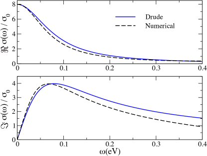
Figure 3: Fit of numerical optical conductivity data with the Drude Model for $\mu=0.5$ eV$where\hbar/\tau=0.07$ eV is the adjustable parameter. The spectral weight is given by $\sigma_{\textrm{D},0}(T,\mu)=\frac{2e^{2}\tau k_{B}T}{\pi\hbar}\log\Big{[}2\cosh\big{[}\frac{\mu}{2k_{B}T}\big{]}\Big{]}$

On the contrary, for values of the Fermi energy where the Drude peak is supressed, the imaginary part of the conductivity is always negative in the entire frequency range (see Fig. 2). This fact has profound consequences in the interaction of graphene with electromagnetic radiation. Just to give an example, when $\Im\sigma(\omega)<0$, graphene does not support $p$-polarized surface waves. On the contrary, for the case of a well-defined Drude peak both $p-$ and $s-$polarized waves are supported, albeit in different frequency ranges ReviewPlasmG_13 .

The reflection coefficients of a graphene sheet are determined by its optical response. Therefore, we expect that the behavior of the Casimir–Polder interaction to be strongly dependent on the details of the optical conductivity, as those discussed above. Specifically, we expect that for the cases where the Drude peak was been washed out the curves of the Casimir–Polder interaction should bunch, whereas for the case where the Drude peak is well defined such bunching should not occur. This is because, in the former case, all conductivity curves essentially coalesce among themselves.

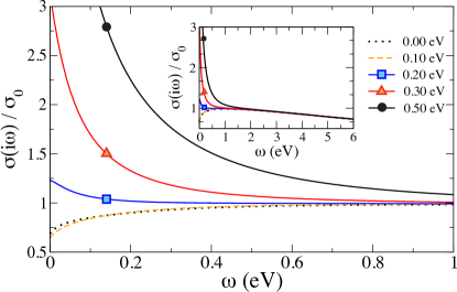
Figure 4: Conductivity in the imaginary frequency axis at selected values of the Fermi energy. The inset shows the same curves over a wider range of frequencies.

The two regimes discussed above, that is $\mu<\mu^{\ast}$ and $\mu>\mu^{\ast}$, become quite clear when the optical conductivity is represented in terms of Matsubara frequencies, as shown in Fig. 4. In this figure, the regime where a Drude peak is well define is characterized by an optical conductivity that presents a positive curvature, whereas in the opposite case the curvature is negative. Therefore, this way of representing the optical conductivity data is an effective tool for separating the two regimes.

III Computation of Casimir–Polder interaction

Here we compute the Casimir–Polder (CP) energy between an atom and a graphene sheet with vacancies and discuss the changes in the CP energy with doping. The optical properties of graphene, necessary for the calculations, can be well described by the numerical results presented in the previous section. We consider a rubidium atom placed at a distance $z$ above a suspended graphene sheet with chemical potential $\mu$. The whole system is assumed to be in thermal equilibrium at sufficiently low temperature $T$, such that one can use the conductivity numerical calculations carried out at $T=0$ K. We choose the rubidium atom due to existence of experimental data of its electric polarizability for wide range of frequencies Rubidium . The CP energy interaction is calculated within the scattering approach Paulo1

$$U_{T}(z) = \frac{k_{B}T}{\varepsilon_{0}c^{2}}{\sum_{l=0}^{\infty}}^{\prime}\xi_{l}^{2}\,\alpha(i\xi_{l})\int\frac{d^{2}\textbf{k}}{(2\pi)^{2}}\frac{e^{-2\kappa_{l}z}}{2\kappa_{l}}$$ (9)

$$\times\Bigg{[}r^{s,s}(\textbf{k},i\xi_{l},\mu)-\Bigg{(}1+\frac{2c^{2}k^{2}}{\xi_{l}^{2}}\Bigg{)}r^{p,p}(\textbf{k},i\xi_{l},\mu)\Bigg{]}\,,$$

where $\xi_{l}=2\pi lk_{B}T/\hbar$ are bosonic Matsubara frequencies, $\kappa_{l}=\sqrt{\xi_{l}^{2}/c^{2}+k^{2}}$, $\alpha(i\xi)$ is the electric polarizability of rubidium, and $r^{s,s}(\textbf{k},i\xi,\mu)$, $r^{p,p}(\textbf{k},i\xi,\mu)$ are the diagonal reflection coefficients associated with graphene. In Eq. (9), the prime indicates that the first term of the summation ($l=0$) is halved.

By modeling graphene as a two-dimensional material with a surface density current ${\bf K}=\mbox{{${\sigma}$}}\cdot{\bf E}|_{z=0}$, and applying the appropriate boundary conditions to the electromagnetic field, the reflections coefficients are calculated as

$$r^{s,s}({\bf k},i\xi,\mu)=\dfrac{2\sigma_{xx}(i\xi,\mu)Z^{h}+\eta_{0}^{2}\sigma_{xx}(i\xi,\mu)^{2}}{-\Delta({\bf k},i\xi,\mu)}\,,$$ (10)

$$r^{p,p}({\bf k},i\xi,\mu)=\dfrac{2\sigma_{xx}(i\xi,\mu)Z^{e}+\eta_{0}^{2}\sigma_{xx}(i\xi,\mu)^{2}}{\Delta({\bf k},i\xi,\mu)}\,,$$ (11)

$$\Delta({\bf k},i\xi,\mu)=[2+Z^{h}\sigma_{xx}(i\xi,\mu)][2+Z^{e}\sigma_{xx}(i\xi,\mu)],$$ (12)

where $Z^{h}=\xi\mu_{0}/\kappa$, $Z^{e}=\kappa/(\xi\epsilon_{0})$, $\eta_{0}^{2}=\mu_{0}/\epsilon_{0}$, and $\sigma_{xx}(i\xi,\mu)$ is the longitudinal optical conductivity of graphene MacdonaldPRL ; booknuno . In the absence of an external magnetic field, the transverse optical conductivity of graphene with vacancies vanishes.

A key point for the computation of the CP energy is the correct modelling of the material surface. In our approach, the characteristics of the material are incorporated in the longitudinal optical conductivity $\sigma_{xx}(\omega)$. Far from the Dirac point, Drude’s model is expected to work for frequencies smaller than the chemical potential. However, for low values of $\mu$, a more accurate calculation must be carried out to capture the detailed physics of graphene and the effects of disorder. In our approach, we use the optical conductivity calculated numerically from a tight-binding Hamiltonian of graphene with vacancies. For that purpose, we first use the Kramers-Kronig relations to obtain the conductivities in the imaginary frequency axis. As shown in Fig. 4, in that case, the separation between the two regimes becomes more clear with different characteristic curve inflections for each regime at for low frequencies.

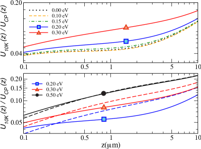
Figure 5: Casimir Polder energy between a rubidium atom and a graphene sheet with $0.4\%$ of randomly distributed vacancies normalized by the CP energy between an atom and a metal plate as function of the distance $z$ between the atom and the graphene layer for different values of the Fermi energy. The lower panel shows the comparison between the energy obtained with the numerical calculation (solid lines) and Drude’s model (dashed Lines).

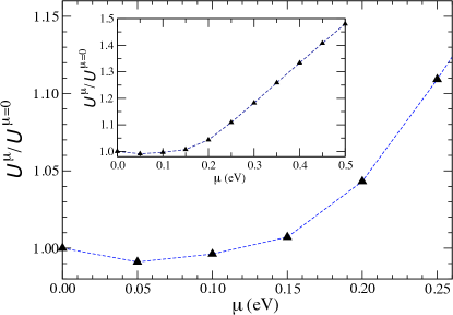
Figure 6: CP energy for finite $\mu$ normalized by CP energy for $\mu=0$ at $z=2\mu m$ as function of chemical potential.

Using equations (9-12) and the optical conductivities shown in Fig. 4, we calculate the CP interaction energy between the graphene sheet and a rubidium atom. Figure 5 presents the CP energy normalized by the interaction between an atom and a perfect metallic surface ($U_{CP}(d)=\frac{-3\hbar c\alpha(0)}{32\pi^{2}\epsilon_{0}d^{4}}$), as a function of the distance at selected values of $\mu$ and $T$=10K. For $\mu<\mu^{*}$, graphene behaves basically as a dieletric and there is a bunching of the CP energy curves. In the opposite regime, the curves are well separated, as expected from the simple Drude model [Eq. (8)]. The lower panel shows a comparison between the CP energy calculated using the numerical data and the Drude model for graphene. Although the optical conductivity curves present a Drude peak for $\mu>\mu^{*}$, the Drude model does not fit well the numerical results for the CP energy, overestimating the CP force for experimentally accessible distances. Saying it differently, our calculations put stringent constrains on the values of the Fermi energy needed to observe the CP effect on graphene. If these are too small the force is also small and one may not be able to measure the effect.

We show in Fig. 6 the variation of CP energy as function of the Fermi energy for $z=2\mu$m. The strong effect of the vacancies, reliably captured by the numerical calculation, results in an almost constant CP energy for a large range of $\mu$ around the Dirac point. For larger values of $\mu$, graphene behaves as a Dirac metal, leading to the linear increase of CP energy as a function of $\mu$ (see inset). For $\mu$=0.50 eV, the CP energy is increased by $50\%$ if compared to the neutrality point.

It is clear from our results that the dependency of CP force with the Fermi energy can be tailored by considering different types of disorder like adatoms and clusters or a higher concentration of vacancies and can become a route to manipulate the behavior of dispersive interactions.

IV Conclusion

In this work we have performed realistic large-scale calculations of the optical conductivity of graphene, revealing the role of disorder for “small” Fermi energies. Our calculations show that in the latter regime, the Drude peak is washed out by disorder and the application of the Drude conductivity for describing the intra-band optical conductivity of graphene becomes unjustifiable. This is an important result, as experiments have been conducted with Fermi energies around $0.2$ eV, where our calculations show that the Drude model is no longer valid. As expected, this behavior has important consequences on the Casimir–Polder effect. For large Fermi energies—$\mu\sim 0.5$ eV—the optical conductivity of graphene is well described by a Drude model at low frequencies. However, at “small” Fermi energies Drude model breaks down and one cannot distinguished the Casimir–Polder interaction energies for varying Fermi energies. Furthermore, the Drude model predicts a larger shift of the interaction energy relative to that of a perfect metallic plane that what will happen in a real situation. Therefore, the forces experienced by the atom will be necessarily smaller than that predicted by the idealized Drude model and may become difficult to measure. Thus for a meaningful experiment our study reveals that highly doped graphene is required.

Appendix

The resolvent operator admits an exact representation in terms of Chebyshev polynomials Ferreira15

$$(z-\hat{h})^{-1}=\sum_{n=0}^{\infty}a_{n}(z)\,\mathcal{T}_{n}(\hat{h})\,,$$ (13)

where $z$ is a complex energy variable with $\Im\,z>0$, $\hat{h}$ is a compact Hamiltonian operator satisfying $||\hat{h}||\leq 1$, and $\mathcal{T}_{n}(\hat{h})$ are Chebyshev polynomials of first kind defined by the recursion relations: $\mathcal{T}_{0}(\hat{h})=1\>,\mathcal{T}_{1}(\hat{h})=\hat{h}$, and

$$\mathcal{T}_{n+1}(\hat{h})=2\hat{h}\,\mathcal{T}_{n}(\hat{h})-\mathcal{T}_{n-1}(\hat{h})\,.$$ (14)

The expansion coefficients are given by

$$a_{n}(z)=\frac{2i^{-1}}{1+\delta_{n,0}}\frac{\left(z-i\sqrt{1-z^{2}}\right)^{n}}{\sqrt{1-z^{2}}}\,.$$ (15)

These results allow us to express the spectral operator in the form given in main text [Eq. (4)].

References

- (1) M. Bordag, U. Mohideen, and V.M. Mostepanenko, Phys. Rep. 353, 1 (2001); K.A. Mil-ton, J. Phys. A 24, R209 (2004); S.K. Lamoreaux, Rep. Prog. Phys. 68, 201 (2005).
- (2) H. B. G. Casimir, Proc. K. Ned. Akad. Wet. 51, 793 (1948).
- (3) H. B. G. Casimir and D. Polder, Nature (London) 158, 787 (1946).
- (4) X. M. H. Huang, C. A. Zorman, M. Mehregany, and M. L. Roukes, Nature 421, 496 (2003).
- (5) M. Aspelmeyer, T. J. Kippenberg, and F. Marquardt, Rev. Mod. Phys. 86, 13911452 (2014).
- (6) L. M. Woods, D. A. R. Dalvit, A. Tkatchenko, P. Rodriguez-Lopez, A. W. Rodriguez, and R. Podgornik, (2015), arXiv:1509.03338 [cond-mat.mtrl-sci].
- (7) G. L. Klimchitskaya, U. Mohideen, V. M. Mostepanenko, Rev. Mod. Phys. 81, 1827 (2009)
- (8) A. H. Castro Neto, F. Guinea, N. M. R. Peres, K. S. Novoselov, and A. K. Geim, Rev. Mod. Phys. 81, 109 (2009).
- (9) N. M. R. Peres, Rev. Mod. Phys. 82, 2673 (2010).
- (10) K. S. Novoselov, V. I. Falko, L. Colombo, P. R. Gellert, M. G. Schwab, K. Kim, Nature 490, 192 (2012).
- (11) M. Bordag, I.V. Fialkovsky, D.M. Gitman and D.V. Vassilevich, Phys. Rev. B 80, 245406 (2009).
- (12) G. Gómez-Santos, Phys. Rev. B 80, 245424 (2009).
- (13) V. Svetovoy, Z. Moktadir, M. Elwenspoek and H. Mizuta, Europhys. Lett. 96, 14006 (2011).
- (14) I.V. Fialkovsky, V.N. Marachevsky and D.V. Vassilevich, Phys. Rev. B 84, 035446 (2011).
- (15) D. Drosdoff and L.M. Wooks, Phys. Rev. A 84, 062501 (2011).
- (16) B.E. Sernelius, Phys. Rev. B 85, 195427 (2012).
- (17) M. Bordag, G.L. Klimchitskaya and V.M. Mostepanenko, Phys. Rev. B 86, 165429 (2012).
- (18) G.L. Klimchitskaya and V.M. Mostepanenko, Phys. Rev. B 87, 075439 (2013).
- (19) G. L. Klimchitskaya and V. M. Mostepanenko, Phys. Rev. B 89, 035407 (2014).
- (20) W.-K. Tse and A. H. MacDonald, Phys. Rev. Lett. 109, 236806 (2012).
- (21) M. Bordag, I. Fialkovskiy and D. Vassilevich, Phys. Rev. B 93, 075414 (2016)
- (22) D. Drosdoff, A. D.Phan, L. M. Woods, I.V.Bondarev, and J.F. Dobson, Eur. Phys. J. B 85, 365 (2012).
- (23) G. L. Klimchitskaya, U. Mohideen, and V. M. Mostepanenko, Phys. Rev. B 89, 115419 (2014).
- (24) Yu V. Churkin, A. B. Fedortsov, G. L. Klimchitskaya and V. A. Yurova, Phys. Rev. B 82, 165433 (2010).
- (25) T. E. Judd, R.G. Scott, A.M. Martin, B. Kaczmarek and T.M. Frohold, New J. Phys.13, 083020 (2011).
- (26) M. Chaichian, G. L. Klimchitskaya, V. M. Mostepanenko and A. Tureanu, Phys. Rev. A 86, 012515 (2012).
- (27) S. Ribeiro and S. Scheel, Phys. Rev. A 88, 042519 (2013); Erratum: Phys. Rev. A 89, 039904 (2014).
- (28) T. Cysne, W. J. M. Kort-Kamp, D. Oliver, F. A. Pinheiro, F. S. S. Rosa , and C. Farina, Phys. Rev. A. 90, 052511 (2014)
- (29) N. Khusnutdinov, R. Kashapov, and L. M. Woods, (2016), arXiv:1602.08443v1 [cond-mat.mes-hall]
- (30) A. Ambrosetti, N. Ferri, R. A. DiStasio Jr., and A. Tkatchenko, Science 351, 1171 (2016).
- (31) P. R.-Lopez, and A. G. Grushin, Phys. Rev. Lett. 112, 056804 (2014).
- (32) F. Huttmann, et al. Phys. Rev. Lett. 115, 236101 (2015)
- (33) A. Ferreira, and E. Mucciolo, Phys. Rev. Lett. 115, 106601 (2015).
- (34) A. H. Castro Neto, F. Guinea, N. M. R. Peres, K. S. Novoselov, and A. K. Geim, Rev. Mod. Phys. 81, 109 (2009).
- (35) G. D. Mahan, Many Particle Physics (Plenum Press, New York, 1981).
- (36) D. J. Thouless and S. Kirkpatrick, J. Phys. C 14, 235 (1981).
- (37) Y. Imry, Introduction to mesoscopic physics, 2nd edition (Oxford University Press, New York, 2002).
- (38) H. Tal-Ezer and R. Kosloff, J. Chem. Phys. 81, 3967 (1984).
- (39) S. Roche, and D. Mayou, Phys. Rev. Lett. 79, 2518 (1997).
- (40) H. Tanaka, Phys. Rev. B 57, 2168 (1998).
- (41) A. Weisse, Eur. Phys. J. B 40, 125 (2004).
- (42) S. Yuan, H. De Raedt, and M. I. Katsnelson, Phys. Rev. B 82, 115448 (2010).
- (43) A. Holzner et al., Phys. Rev. B 83, 195115 (2011).
- (44) A. Weisse, G. Wellein, A. Alvermann, and H. Fehske, Rev. Mod. Phys. 78, 275 (2006).
- (45) N. Leconte, A. Ferreira, and J. Jung, 2D Materials, Elsevier, Vol. 95, 35 (2016).
- (46) A. Ferreira et al., Phys. Rev. B 83, 165402 (2011).
- (47) Z. Fan, A. Uppstu, and A. Harju, Phys. Rev. B 89, 245422 (2014)
- (48) J. H. García, L. Covaci, and T. G. Rappoport, Phys. Rev. Lett. 114, 116602 (2015).
- (49) T. Stauber, N. M. R. Peres, and A. K. Geim Phys. Rev. B 78, 085432 (2008).
- (50) N. M. R. Peres, J. M. B. Lopes dos Santos, and T. Stauber, Phys. Rev. B 76, 073412 (2007).
- (51) Jason Horng, Chi-Fan Chen, Baisong Geng, Caglar Girit, Yuanbo Zhang, Zhao Hao, Hans A. Bechtel, Michael Martin, Alex Zettl, Michael F. Crommie, Y. Ron Shen, and Feng Wang Phys. Rev. B 83, 165113 (2011).
- (52) Y. V. Bludov, A Ferreira, N. M. R Peres, M. I. Vasilevskiy, Int. J. Mod. Phys. B 27, 1341001 (2013).
- (53) A. Derevianko, S. G. Porsev, and J. F. Babb, At. Data Nucl. Data Tables 96, 323 (2010).
- (54) A. M. Contreras-Reyes, R. Guï¿œrout, P. A. Maia Neto, D. A. R. Dalvit, A. Lambrecht, and S. Reynaud, Phys. Rev. A 82, 052517 (2010).
- (55) P.A.D. Gonçalves and N. M. R. Peres, An Introduction to Graphene Plasmonics, (World Scientific, 2016, Singapore).