Optimal Control of Connected Automated Vehicles at Urban Traffic Intersections: A Feasibility Enforcement Analysis

Abstract

Earlier work has established a decentralized optimal control framework for coordinating on line a continuous flow of Connected Automated Vehicles (CAVs) entering a “control zone” and crossing two adjacent intersections in an urban area. A solution, when it exists, allows the vehicles to minimize their fuel consumption while crossing the intersections without the use of traffic lights, without creating congestion, and under the hard safety constraint of collision avoidance. We establish the conditions under which such solutions exist and show that they can be enforced through an appropriately designed “feasibility enforcement zone” that precedes the control zone. The proposed solution and overall control architecture are illustrated through simulation.

I Introduction

Connected and automated vehicles (CAVs) provide significant new opportunities for improving transportation safety and efficiency using inter-vehicle as well as vehicle-to-infrastructure communication [1]. To date, traffic lights are the prevailing method used to control the traffic flow through an intersection. More recently, however, data-driven approaches have been developed leading to online adaptive traffic light control as in [2]. Aside from the obvious infrastructure cost and the need for dynamically controlling green/red cycles, traffic light systems also lead to problems such as significantly increasing the number of rear-end collisions at an intersection. These issues have provided the motivation for drastically new approaches capable of providing a smoother traffic flow and more fuel-efficient driving while also improving safety.

The advent of CAVs provides the opportunity for such new approaches. Dresner and Stone [3] proposed a scheme for automated vehicle intersection control based on the use of reservations whereby a centralized controller coordinates a crossing schedule based on requests and information received from the vehicles located inside some communication range. The main challenges in this case involve possible deadlocks and heavy communication requirements which can become critical. There have been numerous other efforts reported in the literature based on such a reservation scheme [4, 5, 6].

Increasing the throughput of an intersection is one desired goal which can be achieved through the travel time optimization of all vehicles located within a radius from the intersection. Several efforts have focused on minimizing vehicle travel time under collision-avoidance constraints [7, 8, 9, 10]. Lee and Park [11] proposed a different approach based on minimizing the overlap in the position of vehicles inside the intersection rather than their arrival times. Miculescu and Karaman [12] used queueing theory and modeled an intersection as a polling system where vehicles are coordinated to cross without collisions. There have been also several research efforts to address the problem of vehicle coordination at intersections within a decentralized control framework. A detailed discussion of the research in this area reported in the literature to date can be found in [13].

Our earlier work [14] has established a decentralized optimal control framework for coordinating online a continuous flow of CAVs crossing two adjacent intersections in an urban area. We refer to an approach as “centralized” if there is at least one task in the system that is globally decided for all vehicles by a single central controller. In contrast, in a “decentralized” approach, a coordinator may be used to handle or distribute information available in the system without, however, getting involved in any control task. The framework in [14] solves an optimal control problem for each CAV entering a specified Control Zone (CZ) which subsequently regulates the acceleration/deceleration of the CAV. The optimal control problem involves hard safety constraints, including rear-end collision avoidance. These constraints make it nontrivial to ensure the existence of a feasible solution to this problem. In fact, it is easy to check that the rear-end collision avoidance constraints cannot be guaranteed to hold throughout the CZ under an optimal solution unless the initial conditions (time and speed) of each CAV entering the CZ satisfy certain conditions. It is, therefore, of fundamental importance to determine these feasibility conditions and ensure that they can be satisfied.

The contributions of this paper are twofold. First, we study the feasibility conditions required to guarantee a solution of the optimal control problem for each CAV; these are expressed in terms of a feasible region defined in the space of the CAV’s speed and arrival time at the CZ. Second, we introduce a Feasibility Enforcement Zone (FEZ) which precedes the CZ and within which a CAV is controlled with the goal of attaining a point in the feasible region determined by the current state of the CZ. This subsequently guarantees that all required constraints are satisfied when the CAV enters the CZ under an associated optimal control. We emphasize again that the benefits of an optimal controller maximizing throughput and minimizing fuel consumption can only be realized subject to ensuring feasible initial conditions to the optimization problem under consideration.

The structure of the paper is as follows. In Section II, we review the model in [14] and its generalization in [15]. In Section III, we present the CAV coordination framework and associated optimal control problems and solutions considering control/state constraints. In Section IV, we carry out the analysis necessary to identify a feasible region for the initial conditions of each CAV when entering the CZ. In Section V, we develop a design procedure for the FEZ and in Section VI, we include simulation results. We offer concluding remarks in Section VII.

II The Model

We briefly review the model introduced in [14] and [15] where there are two intersections, 1 and 2, located within a distance $D$ (Fig. 1). The region at the center of each intersection, called Merging Zone (MZ), is the area of potential lateral CAV collision. Although it is not restrictive, this is taken to be a square of side $S$. Each intersection has a Control Zone (CZ) and a coordinator that can communicate with the CAVs traveling within it. The distance between the entry of the CZ and the entry of the MZ is $L>S$, and it is assumed to be the same for all entry points to a given CZ.

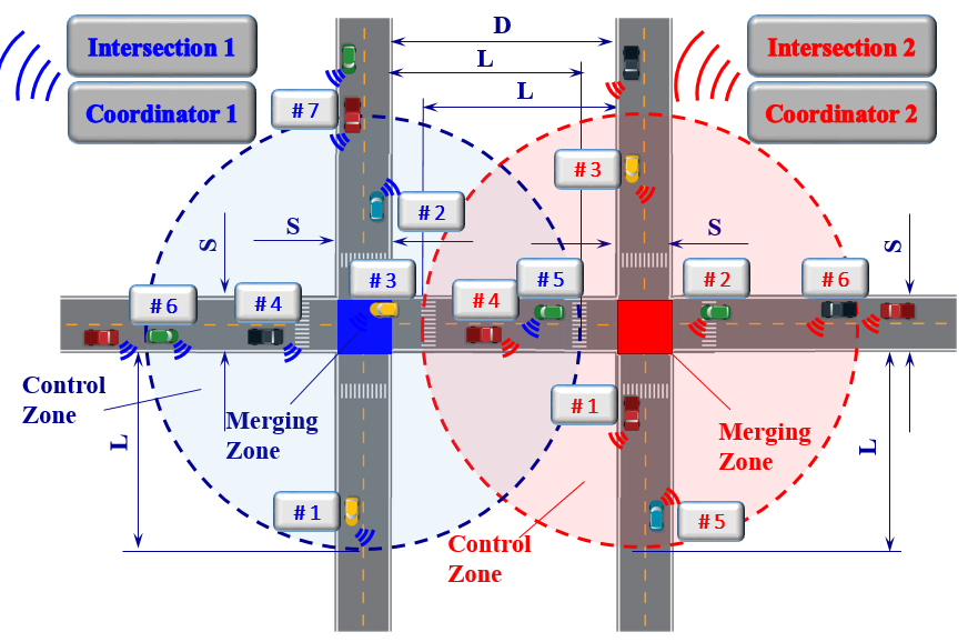
Figure 1: Two intersections with connected and automated CAVs.

Let $M_{z}(t)\in\mathbb{N}$ be the cumulative number of CAVs which have entered the CZ and formed a first-in-first-out (FIFO) queue by time $t$, $z=1,2$. When a CAV reaches the CZ of intersection $z$, the coordinator assigns it an integer value $i=M_{z}(t)+1$. If two or more CAVs enter a CZ at the same time, then the corresponding coordinator selects randomly the first one to be assigned the value $M_{z}(t)+1$. In the region between the exit point of a MZ and the entry point of the subsequent CZ, the CAVs cruise with the speed they had when they exited that MZ.

For simplicity, we assume that each CAV is governed by second order dynamics

$$\dot{p}_{i}=v_{i}(t)\text{, }~{}p_{i}(t_{i}^{0})=0\text{; }~{}\dot{v}_{i}=u_{i}(t)\text{, }v_{i}(t_{i}^{0})\text{ given}$$ (1)

where $p_{i}(t)\in\mathcal{P}_{i}$, $v_{i}(t)\in\mathcal{V}_{i}$, and $u_{i}(t)\in\mathcal{U}_{i}$ denote the position, i.e., travel distance since the entry of the CZ, speed and acceleration/deceleration (control input) of each CAV $i$. These dynamics are in force over an interval $[t_{i}^{0},t_{i}^{f}]$, where $t_{i}^{0}$ is the time that CAV $i$ enters the CZ and $t_{i}^{f}$ is the time that it exits the MZ of intersection $z$.

To ensure that the control input and vehicle speed are within a given admissible range, the following constraints are imposed:

$$\begin{split}u_{i,min}&\leqslant u_{i}(t)\leqslant u_{i,max},\quad\text{and}\\ 0&\leqslant v_{min}\leqslant v_{i}(t)\leqslant v_{max},\quad\forall t\in[t_{i}^{0},t_{i}^{m}],\end{split}$$ (2)

To ensure the absence of any rear-end collision throughout the CZ, we impose the rear-end safety constraint

$$s_{i}(t)=p_{k}(t)-p_{i}(t)\geqslant\delta,\quad\forall t\in[t_{i}^{0},t_{i}^{m}]$$ (3)

where $\delta$ is the minimal safe distance allowable and $k$ is the CAV physically ahead of $i$.

As part of safety considerations, we impose the following assumption (which may be relaxed if necessary):

Assumption 1

The speed of the CAVs inside the MZ is constant, i.e., $v_{i}(t)=v_{i}(t_{i}^{m})=v_{i}(t_{i}^{f})$, $\ \forall t\in[t_{i}^{m},t_{i}^{f}]$, where $t_{i}^{m}$ is the time that CAV $i$ enters the MZ of the intersection. This implies that

$$t_{i}^{f}=t_{i}^{m}+\frac{S}{v_{i}(t_{i}^{m})}.$$ (4)

The objective of each CAV is to derive an optimal acceleration/deceleration in terms of fuel consumption over the time interval $[t_{i}^{0},t_{i}^{m}]$ while avoiding congestion between the two intersections. In addition, we impose hard constraints so as to avoid either rear-end collision, or lateral collision inside the MZ. In fact, it is shown in [15] that the centralized throughput maximization problem is equivalent to a set of decentralized problems whereby each CAV minimizes its fuel consumption as long as the safety constraints applying to it are satisfied. Thus, in what follows, we focus on these decentralized problems and their associated safety constraints.

III Vehicle Coordination and Control

III-A Decentralized Control Problem Formulation

Since the coordinator is not involved in any decision on the vehicle control, we can formulate $M_{1}(t)$ and $M_{2}(t)$ decentralized tractable problems for intersection 1 and 2 respectively that may be solved on line. When a CAV enters a CZ, $z=1,2$, it is assigned a pair $(i,j)$ from the coordinator, where $i=M_{z}(t)+1$ is a unique index and $j$ indicates the positional relationship between CAVs $i-1$ and $i$. As formally defined in [14], with respect to CAV $i$, CAV $i-1$ belongs to one and only one of the four following subsets: $(i)$ $\mathcal{R}_{i}^{z}(t)$ contains all CAVs traveling on the same road as $i$ and towards the same direction but on different lanes, $(ii)$ $\mathcal{L}_{i}^{z}(t)$ contains all CAVs traveling on the same road and lane as CAV $i$, $(iii)$ $\mathcal{C}_{i}^{z}(t)$ contains all CAVs traveling on different roads from $i$ and having destinations that can cause lateral collision at the MZ, and $(iv)$ $\mathcal{O}_{i}^{z}(t)$ contains all CAVs traveling on the same road as $i$ and opposite destinations that cannot, however, cause collision at the MZ. Note that the FIFO structure of this queue implies the following condition:

$$t_{i}^{m}\geqslant t_{i-1}^{m},~{}i>1.$$ (5)

Under the assumption that each CAV $i$ has proximity sensors and can observe and/or estimate local information that can be shared with other CAVs, we define its information set $Y_{i}(t)$, $t\in[t_{i}^{0},t_{i}^{f}]$, as

$$Y_{i}(t)\triangleq\Big{\{}p_{i}(t),v_{i}(t),\mathcal{Q}_{j}^{z},j=1,\ldots,4,z=1,2,s_{i}(t),t_{i}^{m}\Big{\}},$$ (6)

where $p_{i}(t),v_{i}(t)$ are the position and speed of CAV $i$ inside the CZ it belongs to, and $\mathcal{Q}_{j}^{z}\in\{\mathcal{R}_{i}^{z}(t),$ $\mathcal{L}_{i}^{z}(t),$ $\mathcal{C}_{i}^{z}(t),$ $\mathcal{O}_{i}^{z}(t)\},$ $z=1,2,$ is the subset assigned to CAV $i$ by the coordinator. The fourth element in $Y_{i}(t)$ is $s_{i}(t)=p_{k}(t)-p_{i}(t)$, the distance between CAV $i$ and CAV $k$ which is immediately ahead of $i$ in the same lane (the index $k$ is made available to $i$ by the coordinator). The last element above, $t_{i}^{m}$, is the time targeted for CAV $i$ to enter the MZ, whose evaluation is discussed next. Note that once CAV $i$ enters the CZ, then all information in $Y_{i}(t)$ becomes available to $i$.

The time $t_{i}^{m}$ that CAV $i$ is required to enter the MZ is based on maximizing the intersection throughput while satisfying (5) and the constraints for avoiding rear-end and lateral collision in the MZ. There are three cases to consider regarding $t_{i}^{m}$, depending on the value of $\mathcal{Q}_{j}^{z}$:

Case 1: $(i-1)\in\mathcal{R}_{i}^{z}(t)\cup\mathcal{O}_{i}^{z}(t):$ in this case, none of the safety constraints can become active while $i$ and $i-1$ are in the CZ or MZ. This allows CAV $i$ to minimize its time in the CZ while preserving the FIFO queue through $t_{i}^{m}\geqslant t_{i-1}^{m},~{}i>1$. Therefore, it is obvious that we should set

$$t_{i}^{m}=t_{i-1}^{m}$$ (7)

and since CAV speeds inside the MZ are constant (Assumption 1), both $i-1$ and $i$ will also be exiting the MZ at the same time by setting

$$v_{i}^{m}=v_{i-1}^{m}.$$ (8)

where $v_{i}^{m}=v_{i}(t_{i}^{m})$ and $v_{i-1}^{m}=v_{i-1}(t_{i-1}^{m})$. Note that, by Assumption 1, $v_{i}(t)=v_{i-1}(t)$ for all $t\in[t_{i}^{m},t_{i}^{f}]$.

Case 2: $(i-1)\in\mathcal{L}_{i}^{z}(t):$ in this case, only the rear-end collision constraint (3) can become active. In order to minimize the time CAV $i$ spends in the CZ by ensuring that (3) is satisfied over $t\in[t_{i}^{m},t_{i-1}^{f}]$ while $v_{i-1}(t)$ is constant (Assumption 1), we set

$$t_{i}^{m}=t_{i-1}^{m}+\frac{\delta}{v_{i-1}^{m}},$$ (9)

and $v_{i}^{m}$ as in (8).

Case 3: $(i-1)\in\mathcal{C}_{i}^{z}(t):$ in this case, only the lateral collision may occur. Hence, CAV $i$ is allowed to enter the MZ only when CAV $i-1$ exits from it. To minimize the time CAV $i$ spends in the CZ while ensuring that the lateral collision avoidance is satisfied over $t\in[t_{i}^{m},t_{i-1}^{f}]$, we set

$$t_{i}^{m}=t_{i-1}^{m}+\frac{S}{v_{i-1}^{m}},$$ (10)

and $v_{i}^{m}$ as in (8).

It follows from (7) through (10) that $t_{i}^{m}$ is always recursively determined from $t_{i-1}^{m}$ and $v_{i-1}^{m}$. Similarly, $v_{i}^{m}$ depends only on $v_{i-1}^{m}$.

Although (7), (9), and (10) provide a simple recursive structure for determining $t_{i}^{m}$, the presence of the control and state constraints (2) may prevent these values from being admissible. This may happen by (2) becoming active at some internal point during an optimal trajectory (see [15] for details). In addition, however, there is a global lower bound to $t_{i}^{f}$, hence also $t_{i}^{m}$ through (4), which depends on $t_{i}^{0}$ and on whether CAV $i$ can reach $v_{max}$ prior to $t_{i-1}^{m}$ or not: $(i)$ If CAV $i$ enters the CZ at $t_{i}^{0}$, accelerates with $u_{i,max}$ until it reaches $v_{max}$ and then cruises at this speed until it leaves the MZ at time $t_{i}^{1}$, it was shown in [14] that

$$t_{i}^{1}=t_{i}^{0}+\frac{L+S}{v_{max}}+\frac{(v_{max}-v_{i}^{0})^{2}}{2u_{i,max}v_{max}}.$$ (11)

$(ii)$ If CAV $i$ accelerates with $u_{i,max}$ but reaches the MZ at $t_{i}^{m}$ with speed $v_{i}^{m}<v_{max}$, it was shown in [14] that

$$t_{i}^{2}=t_{i}^{0}+\frac{v_{i}(t_{i}^{m})-v_{i}^{0}}{u_{i,max}}+\frac{S}{v_{i}^{m}},$$ (12)

where $v_{i}(t_{i}^{m})=\sqrt{2Lu_{i,max}+(v_{i}^{0})^{2}}$. Thus,

$$t_{i}^{c}=t_{i}^{1}\mathbbm{1}_{v_{i}^{m}=v_{max}}+t_{i}^{2}(1-\mathbbm{1}_{v_{i}^{m}=v_{max}})$$

is a lower bound of $t_{i}^{f}$ regardless of the solution of the problem. Therefore, we can summarize the recursive construction of $t_{i}^{f}$ over $i=1,\ldots,M_{z}(t)$ as follows:

$$t_{i}^{f}=\left\{\begin{array}[c]{ll}t_{1}^{f},&\mbox{if $i=1$},\\ \text{max }\{t_{i-1}^{f},t_{i}^{c}\},&\text{if }i-1\in\mathcal{R}_{i}^{z}(t)\cup\mathcal{O}_{i}^{z}(t)\\ \text{max }\{t_{i-1}^{f}+\frac{\delta}{v_{i}(t_{i-1}^{f})},t_{i}^{c}\},&\mbox{if $i-1\in\mathcal{L}_{i}^{z}$},\\ \text{max }\{t_{i-1}^{f}+\frac{S}{v_{i}(t_{i-1}^{f})},t_{i}^{c}\},&\mbox{if $i-1\in\mathcal{C}_{i}^{z}$},\end{array}\right.$$ (13)

where $t_{i}^{m}$ can be evaluated from $t_{i}^{f}$ through (4), and thus, it is always feasible.

Note that at each time $t$, each CAV $i$ communicates with the preceding CAV $i-1$ in the queue and accesses the values of $t_{i-1}^{f}$, $v_{i-1}(t_{i-1}^{f})$, $\mathcal{Q}_{j}^{z}$, $j=1,\dots,4$, $z=1,2$ from its information set in (6). This is necessary for $i$ to compute $t_{i}^{f}$ appropriately and satisfy (13) and (3). The following result is established in [14] to formally assert the iterative structure of the sequence of decentralized optimal control problems:

Lemma 1

The decentralized communication structure aims for each CAV $i$ to solve an optimal control problem for $t\in[t_{i}^{0},t_{i}^{m}]$ the solution of which depends only on the solution of CAV $i$-1.

The decentralized optimal control problem for each CAV approaching either intersection is formulated so as to minimize the $L^{2}$-norm of its control input (acceleration/deceleration). It has been shown in [16] that there is a monotonic relationship between fuel consumption for each CAV $i$, and its control input $u_{i}$. Therefore, we formulate the following problem for each $i$:

$$\min_{u_{i}\in U_{i}}\frac{1}{2}\int_{t_{i}^{0}}^{t_{i}^{m}}K_{i}\cdot u_{i}^{2}~{}dt$$

$$\text{subject to}:\eqref{eq:model2},(\ref{speed_accel constraints}),(\ref{eq:time}),\eqref{def:tf},\text{ }p_{i}(t_{i}^{0})=0\text{, }p_{i}(t_{i}^{m})=L,$$ (14)

$$z=1,2,\text{and given }t_{i}^{0}\text{, }v_{i}(t_{i}^{0}).$$

where $K_{i}$ is a factor to capture CAV diversity (for simplicity we set $K_{i}=1$ for the rest of this paper). Note that this formulation does not include the safety constraint (3).

III-B Analytical solution of the decentralized optimal control problem

An analytical solution of problem (14) may be obtained through a Hamiltonian analysis. The presence of constraints (2) and (13) complicates this analysis. Assuming that all constraints are satisfied upon entering the CZ and that they remain inactive throughout $[t_{i}^{0},t_{i}^{m}]$, a complete solution was derived in [16] and [17] for highway on-ramps, and in [14] for two adjacent intersections. This solution is summarized next (the complete solution including any constraint (2) becoming active is given in [15]). The optimal control input (acceleration/deceleration) over $t\in[t_{i}^{0},t_{i}^{m}]$ is given by

$$u_{i}^{\ast}(t)=a_{i}t+b_{i}$$ (15)

where $a_{i}$ and $b_{i}$ are constants. Using (15) in the CAV dynamics (1) we also obtain the optimal speed and position:

$$v_{i}^{\ast}(t)=\frac{1}{2}a_{i}t^{2}+b_{i}t+c_{i}$$ (16)

$$p_{i}^{\ast}(t)=\frac{1}{6}a_{i}t^{3}+\frac{1}{2}b_{i}t^{2}+c_{i}t+d_{i},$$ (17)

where $c_{i}$ and $d_{i}$ are constants of integration. The constants $a_{i}$, $b_{i}$, $c_{i}$, $d_{i}$ can be computed by using the given initial and final conditions. The interdependence of the two intersections, i.e., the coordination of CAVs at the MZ of one intersection which affects the behavior of CAV coordination of the other MZ, is discussed in [14].

We note that the control of CAV $i$ actually remains unchanged until an “event” occurs that affects its behavior. Therefore, the time-driven controller above can be replaced by an event-driven one without affecting its optimality properties under conditions described in [18].

As already mentioned, the analytical solution (15) is only valid as long as all initial conditions satisfy (2) and (13) and these constraints continue to be satisfied throughout $[t_{i}^{0},t_{i}^{m}]$. Otherwise, the solution needs to be modified as described in [15].

Recall that the constraint (3) is not included in (14) and it is a much more challenging matter. To deal with this, we proceed as follows. First, we analyze under what initial conditions $(t_{i}^{0},v_{i}^{0})$ the constraint is violated upon CAV $i$ entering the CZ. This defines a feasibility region in the $(t_{i}^{0},v_{i}^{0})$ space which we denote by $\mathcal{F}_{i}$. Assuming the CAV has initial conditions which are feasible, we then derive a condition under which the CAV’s state maintains feasibility over $[t_{i}^{0},t_{i}^{m}]$. Finally, we explore how to enforce feasibility at the time of CZ entry, i.e., enforcing the condition $(t_{i}^{0},v_{i}^{0})\in\mathcal{F}_{i}$. This is accomplished by introducing a Feasibility Enforcement Zone (FEZ) which precedes the CZ. If the FEZ is properly designed, we show that $(t_{i}^{0},v_{i}^{0})\in\mathcal{F}_{i}$ can be ensured.

IV Feasibility enforcement analysis

We begin with a simple example of how the safety constraint (3) may be violated under the optimal control (15). This is illustrated in Fig. 2 with $\delta=10$ for two CAVs that follow each other into the same lane in the CZ. We can see that while (3) is eventually satisfied over the MZ, due to the constraints imposed on the solution of (14) through (13), the controller (15) is unable to maintain (3) throughout the CZ. What is noteworthy in Fig. 2 is that (3) is violated by CAV 3 at an interval which is interior to $[t_{3}^{0},t_{3}^{m}]$, i.e., the form of the optimal control solution (15) causes this violation even though the constraint is initially satisfied at $t_{3}^{0}=5$ in Fig. 2.

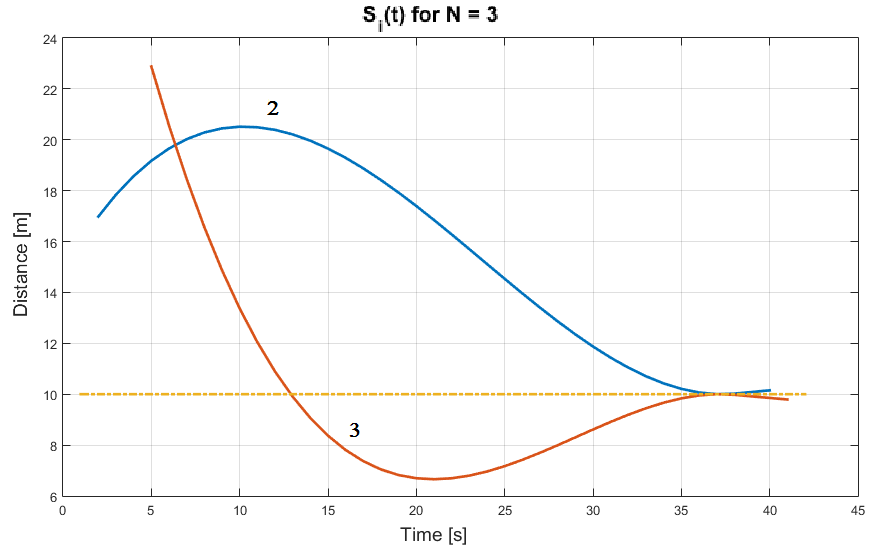
Figure 2: Example of safety constraint violation by CAV 3 when $\delta$ = 10.

Recall that we use $k$ to denote the CAV physically preceding $i$ on the same lane in the CAV, and $i-1$ is the CAV preceding $i$ in the FIFO queue associated with the CAV, we have the following theorem.

Theorem 1

There exists a nonempty feasible region $\mathcal{F}_{i}\subset R^{2}$ of initial conditions $(t_{i}^{0},v_{i}^{0})$ for CAV $i$ such that, under the decentralized optimal control, $s_{i}(t)\geqslant\delta$ for all $t\in[t_{i}^{0},t_{i}^{m}]$ given the initial and final conditions $t_{k}^{0},v_{k}^{0},t_{k}^{m},v_{k}^{m}$ of CAV $k$.

Proof: To prove the existence of the feasible region, there are two cases to consider, depending on whether any state or control constraint for either CAV $i$ or $k$ becomes active in the CZ.

Case 1: No state or control constraint is active for either $k$ or $i$ over $[t_{i}^{0},t_{i}^{m}]$. By using (16), (17) at $t$ and $t_{i}^{m}$, and the definition $s_{i}(t)=p_{k}(t)-p_{i}(t)$, under optimal control we can write

$$s_{i}(t;t_{i}^{0},v_{i}^{0})=s_{i}(t,t_{i}^{m},v_{i}^{m},t_{k}^{0},v_{k}^{0},t_{k}^{m},v_{k}^{m};t_{i}^{0},v_{i}^{0})$$

$$=A(t,t_{i}^{m},v_{i}^{m},t_{k}^{0},v_{k}^{0},t_{k}^{m},v_{k}^{m};t_{i}^{0},v_{i}^{0})t^{3}$$

$$+B(t,t_{i}^{m},v_{i}^{m},t_{k}^{0},v_{k}^{0},t_{k}^{m},v_{k}^{m};t_{i}^{0},v_{i}^{0})t^{2}$$

$$+C(t,t_{i}^{m},v_{i}^{m},t_{k}^{0},v_{k}^{0},t_{k}^{m},v_{k}^{m};t_{i}^{0},v_{i}^{0})t$$

$$+D(t,t_{i}^{m},v_{i}^{m},t_{k}^{0},v_{k}^{0},t_{k}^{m},v_{k}^{m};t_{i}^{0},v_{i}^{0}),$$ (18)

where $A$, $B$, $C$ and $D$ are functions defined over $t\in[t_{i}^{0},t_{i}^{m}]$. Recall that CAV $k$ is cruising in the MZ, so that (15) through (17) do not apply for $k$ over $[t_{k}^{m},t_{i}^{m}]$ leading to different expressions for $A$, $B$, $C$ and $D$. Therefore, we consider two further subcases, one for $[t_{i}^{0},t_{k}^{m}]$ and the other for $[t_{k}^{m},t_{i}^{m}]$. For ease of notation, in the sequel we replace $(t_{i}^{0},v_{i}^{0})$ by $(\tau,\upsilon)$.

Case 1.1: $t\in[t_{i}^{0},t_{k}^{m}]$. In this case, $s_{i}(t;\tau,\upsilon)$ is a cubic polynomial inheriting the cubic structure of (17). We can solve (16), (17) for the cofficients $a_{k}$, $b_{k}$, $c_{k}$, $d_{k}$, $a_{i}$, $b_{i}$, $c_{i}$ and $d_{i}$ using the initial and final conditions of CAVs $k$ and $i$. Then, denoting $A$, $B$, $C$ and $D$ as $A_{1}(\tau,v)$, $B_{1}(\tau,v)$, $C_{1}(\tau,v)$ and $D_{1}(\tau,v)$ for $t\in[t_{i}^{0},t_{k}^{m}]$, these are explicitly given by

$$A_{1}(\tau,\upsilon) =\frac{1}{(t_{k}^{0}-t_{k}^{m})^{3}}(2L+(v_{k}^{m}+v_{k}^{0})(t_{k}^{0}-t_{k}^{m}))$$

$$-\frac{1}{(\tau-t_{i}^{m})^{3}}(2L+(v_{i}^{m}+\upsilon)(\tau-t_{i}^{m})),$$

$$B_{1}(\tau,\upsilon) =-\frac{1}{(t_{k}^{0}-t_{k}^{m})^{3}}[3L(t_{k}^{0}+t_{k}^{m})$$

$$+(v_{k}^{0}(t_{k}^{0}+2t_{k}^{m})+v_{k}^{m}(2t_{k}^{0}+t_{k}^{m}))(t_{k}^{0}-t_{k}^{m})]$$

$$+\frac{1}{(\tau-t_{i}^{m})^{3}}[3L(\tau+t_{i}^{m})$$

$$+(\upsilon(\tau+2t_{i}^{m})+v_{i}^{m}(2\tau+t_{i}^{m}))(\tau-t_{i}^{m})],$$

$$C_{1}(\tau,\upsilon) =\frac{1}{(t_{k}^{0}-t_{k}^{m})^{3}}[6t_{k}^{0}t_{k}^{m}L+[(v_{k}^{0}((t_{k}^{m})^{2}+2t_{k}^{0}t_{k}^{m})$$

$$+v_{k}^{m}((t_{k}^{0})^{2}+2t_{k}^{m}t_{k}^{0}))](t_{k}^{0}-t_{k}^{m})]$$

$$-\frac{1}{(\tau-t_{i}^{m})^{3}}[6\tau t_{i}^{m}L+[(\upsilon((t_{i}^{m})^{2}+2\tau t_{i}^{m})$$

$$+v_{i}^{m}((\tau)^{2}+2t_{i}^{m}\tau))](\tau-t_{i}^{m})],$$

$$D_{1}(\tau,\upsilon) =\frac{1}{(t_{k}^{0}-t_{k}^{m})^{3}}[L((t_{k}^{0})^{3}-3(t_{k}^{0})^{2}t_{k}^{m})$$

$$-(v_{k}^{0}t_{k}^{0}(t_{k}^{m})^{2}+v_{k}^{m}(t_{k}^{0})^{2}t_{k}^{m})(t_{k}^{0}-t_{k}^{m})]$$

$$-\frac{1}{(\tau-t_{i}^{m})^{3}}[L((\tau)^{3}-3(\tau)^{2}t_{i}^{m})$$

$$-(\upsilon\tau(t_{i}^{m})^{2}+v_{i}^{m}(\tau)^{2}t_{i}^{m})(\tau-t_{i}^{m})].$$

Aside from $(\tau,v)$, all remaining arguments are known to CAV $i$ and can be determined. Hence, $s_{i}(t;\tau,v)$ varies only with $t$ and $(\tau,v)$. First, observing that the first half of each of the coefficient expressions in (IV) (which is derived by solving (16) and (17) for CAV $k$) is a constant fully determined by information provided by CAV $k$, we can rewrite these as $K_{A_{1}}$, $K_{B_{1}}$, $K_{C_{1}}$, $K_{D_{1}}$. Therefore, $p_{k}^{\ast}(t)$ in (17) can be expressed as

$$p_{k}^{\ast}(t)=K_{A_{1}}t^{3}+K_{B_{1}}t^{2}+K_{C_{1}}t+K_{D_{1}}.$$ (19)

Next, the second half of the coefficients can be expressed through polynomials in either $\tau$ or $\upsilon$ explicitly derived by solving (16) and (17) for CAV $i$. We will use the notation $P_{X,n}(\tau)$, $P_{X,n}(\upsilon)$ to represent polynomials of degree $n=1,2,3$ and $X\in\{A_{1},B_{1},C_{1},D_{1}\}$. Similarly, we set $Q_{3}(\tau)=(\tau-t_{i}^{m})^{3}$. Thus, for the coefficients in Eq. (IV), we get

$$A_{1}(\tau,\upsilon) =K_{A_{1}}+\frac{P_{A_{1},1}(\tau)P_{A_{1},1}(\upsilon)}{Q_{3}(\tau)},$$ (20)

$$B_{1}(\tau,\upsilon) =K_{B_{1}}+\frac{P_{B_{1},2}(\tau)P_{B_{1},1}(\upsilon)}{Q_{3}(\tau)},$$

$$C_{1}(\tau,\upsilon) =K_{C_{1}}+\frac{P_{C_{1},3}(\tau)+P_{C_{1},2}(\tau)P_{C_{1},1}(\upsilon)}{Q_{3}(\tau)},$$

$$D_{1}(\tau,\upsilon) =K_{D_{1}}+\frac{P_{D_{1},3}(\tau)+P_{D_{1},2}(\tau)P_{D_{1},1}(\upsilon)}{Q_{3}(\tau)}.$$

Note that $p_{k}^{\ast}(t)$ in (19) involves only the $K$ terms, while the analogous cubic polynomial for $p_{i}^{\ast}(t)$ involves only the $P$ and $Q$ terms.

Our goal is to ensure that $s_{i}(t;\tau,\upsilon)\geqslant\delta$ for all $t\in[\tau,t_{k}^{m}]$ (recall that $t_{i}^{0}\equiv\tau$). We can guarantee this by ensuring that $s_{i}^{\ast}(\tau,\upsilon)\equiv\min_{t\in[\tau,t_{k}^{m}]}\{s_{i}(t;\tau,\upsilon)\}\geqslant\delta$. Thus, we shift our attention to the determination of $s_{i}^{\ast}(\tau,\upsilon)$. We can obtain expressions for the first and the second derivative of $s_{i}(t;\tau,\upsilon)$, $\dot{s}_{i}(t;\tau,\upsilon)$ and $\ddot{s}_{i}(t;\tau,\upsilon)$ respectively, from (18), as follows:

$$\dot{s}_{i}(t;\tau,\upsilon) =v_{k}(t)-v_{i}(t)$$ (21)

$$=3A_{1}(\tau,\upsilon)t^{2}+2B_{1}(\tau,\upsilon)t+C_{1}(\tau,\upsilon),$$

$$\ddot{s}_{i}(t;\tau,\upsilon) =u_{k}(t)-u_{i}(t)$$ (22)

$$=6A_{1}(\tau,\upsilon)t+2B_{1}(\tau,\upsilon).$$

Clearly, we can determine $t_{i}^{\ast}\equiv\arg\min_{t\in[\tau,t_{k}^{m}]}\{s_{i}(t;\tau,\upsilon)\}$ as the solution of $\dot{s}_{i}(t;\tau,\upsilon)=0$ with $\ddot{s}_{i}(t;\tau,\upsilon)\geqslant 0$, unless $s_{i}^{\ast}(\tau,\upsilon)$ occurs at the boundaries, i.e., $t_{i}^{\ast}=\tau$ or $t_{i}^{\ast}=t_{k}^{m}$. Thus, there are three cases to consider:

Case 1.1.A: $t_{i}^{\ast}=\tau$. In this case,

$$s_{i}^{\ast}(\tau,\upsilon)=s_{i}(\tau;\tau,\upsilon)$$ (23)

$$=A_{1}(\tau,\upsilon)\tau^{3}+B_{1}(\tau,\upsilon)\tau^{2}+C_{1}(\tau,\upsilon)\tau+D_{1}(\tau,\upsilon)\geqslant\delta$$

and we can satisfy $s_{i}(\tau,\upsilon)\geqslant\delta$ for any $\upsilon$ as long as a feasible $\tau$ is determined. Since at $t=\tau$, we have $p_{i}(\tau)=0$ and using the definition of $s_{i}(t)=p_{k}(t)-p_{i}(t)$ and (19),

$$s_{i}(\tau)=p_{k}^{\ast}(\tau)=K_{A_{1}}\tau^{3}+K_{B_{1}}\tau^{2}+K_{C_{1}}\tau+K_{D_{1}}.$$

Observe that if $p_{k}(\tau)\geqslant\delta$, then CAV $i$ enters the CZ at a safe distance from its preceding CAV $k$ and since $t_{i}^{\ast}=\tau$, we have $s_{i}(t;\tau,\upsilon)\geqslant\delta$ for all $t\in[\tau,t_{k}^{m}]$. Thus, it suffices to select

$$\tau\geqslant t_{k}^{\delta}$$ (24)

where $t_{k}^{\delta}$ is the smallest real root of $p_{k}(\tau)-\delta=0$.

Case 1.1.B: $t_{i}^{\ast}=t_{k}^{m}$. In this case,

$$s_{i}^{\ast}(\tau,\upsilon)=s_{i}(t_{k}^{m};\tau,\upsilon)$$ (25)

$$=A_{1}(\tau,\upsilon)(t_{k}^{m})^{3}+B_{1}(\tau,\upsilon)(t_{k}^{m})^{2}+C_{1}(\tau,\upsilon)t_{k}^{m}$$

$$+D_{1}(\tau,\upsilon)\geqslant\delta$$

Thus, the feasibility region $\mathcal{F}_{i}$ is defined by all $(\tau,\upsilon)$ such that $s_{i}(t_{k}^{m};\tau,\upsilon)-\delta\geqslant 0$ in the $(\tau,\upsilon)$ space.

Case 1.1.C: $t_{i}^{\ast}=t_{1}\in(\tau,t_{k}^{m})$. This case only arises if the determinant $\mathcal{D}_{i}(\tau,\upsilon)$ of (21) is positive, i.e.,

$$\mathcal{D}_{i}(\tau,\upsilon)=4B_{1}(\tau,\upsilon)^{2}-12A_{1}(\tau,\upsilon)C_{1}(\tau,\upsilon)>0$$ (26)

and we get

$$t_{1}=\frac{-2B_{1}(\tau,\upsilon)\pm\sqrt{\mathcal{D}_{i}(\tau,\upsilon)}}{6A_{1}(\tau,\upsilon)}$$ (27)

In addition, we must have

$$\tau<t_{1}<t_{k}^{m},\text{ \ \ }\dot{s}_{i}(t_{1};\tau,\upsilon)=0,\text{ \ \ }\ddot{s}_{i}(t_{1};\tau,\upsilon)\geqslant 0$$ (28)

Therefore, the feasibility region $\mathcal{F}_{i}$ is defined by all $(\tau,\upsilon)$ such that

$$s_{i}^{\ast}(\tau,\upsilon) =s_{i}(t_{1};\tau,\upsilon)$$ (29)

$$=A_{1}(\tau,\upsilon)(t_{1})^{3}+ B_{1}(\tau,\upsilon)(t_{1})^{2}+C_{1}(\tau,\upsilon)t_{1}$$

$$+ D_{1}(\tau,\upsilon)\geqslant\delta$$

in conjunction with (27)-(28).

Case 1.2: $t\in[t_{k}^{m},t_{i}^{m}]$. Over this interval, $v_{k}(t)=v_{k}^{m}$ by Assumption 1. Therefore, (15)-(17) no longer apply: (15) becomes $u_{k}^{\ast}(t)=0$, (16) becomes $v_{k}^{\ast}(t)=v_{k}^{m}$ and (17) becomes $p_{k}^{\ast}(t)=L+v_{k}^{m}(t-t_{k}^{m})$. Evaluating $s_{i}(t)=p_{k}(t)-p_{i}(t)$ in this case yields the following coefficients in (IV):

$$A_{2}(\tau,\upsilon) =-\frac{1}{(\tau-t_{i}^{m})^{3}}(2L+(v_{i}^{m}+\upsilon)(\tau-t_{i}^{m})),$$ (30)

$$B_{2}(\tau,\upsilon) =\frac{1}{(\tau-t_{i}^{m})^{3}}[3L(\tau+t_{i}^{m})+(\upsilon(\tau+2t_{i}^{m})$$

$$+v_{i}^{m}(2\tau+t_{i}^{m}))(\tau-t_{i}^{m})],$$

$$C_{2}(\tau,\upsilon) =v_{k}^{m}-\frac{1}{(\tau-t_{i}^{m})^{3}}[6\tau t_{i}^{m}L+[(\upsilon((t_{i}^{m})^{2}+2\tau t_{i}^{m})$$

$$+v_{i}^{m}((\tau)^{2}+2t_{i}^{m}\tau))](\tau-t_{i}^{m})],$$

$$D_{2}(\tau,\upsilon) =L-v_{k}^{m}t_{k}^{m}-\frac{1}{(\tau-t_{i}^{m})^{3}}[L((\tau)^{3}-3(\tau)^{2}t_{i}^{m})$$

$$-(\upsilon\tau(t_{i}^{m})^{2}+v_{i}^{m}(\tau)^{2}t_{i}^{m})(\tau-t_{i}^{m})].$$

It follows that $K_{A_{1}},K_{B_{1}},K_{C_{1}}$ and $K_{D_{1}}$ in (20) should be modified accordingly, giving $K_{A_{2}}=K_{B_{2}}=0$, $K_{C_{2}}=v_{k}^{m}$ and $K_{D_{2}}=L-v_{k}^{m}t_{k}^{m}$. Since we are assuming that no control or state constraints are active for CAV $i$, the designated final time $t_{i}^{m}$ under optimal control satisfies (9), i.e., $s_{i}(t_{i}^{m})=\delta$. Thus, we only need to consider the subcase where $s_{i}^{\ast}(\tau,\upsilon)$ occurs in $(t_{k}^{m},t_{i}^{m})$ and we have $t_{i}^{\ast}=t_{2}$, $t_{2}\in(t_{k}^{m},t_{i}^{m})$. Proceeding as in Case 1.1.C, the feasibility region $\mathcal{F}_{i}$ is defined by all $(\tau,\upsilon)$ such that

$$s_{i}^{\ast}(\tau,\upsilon)=s_{i}(t_{2};\tau,\upsilon)$$ (31)

$$=A_{2}(\tau,\upsilon)(t_{2})^{3}+B_{2}(\tau,\upsilon)(t_{2})^{2}+C_{2}(\tau,\upsilon)t_{2}$$

$$+D_{2}(\tau,\upsilon)\geqslant\delta$$

in conjunction with (27)-(28), with $A_{1}$, $B_{1}$, $C_{1}$ and $D_{1}$ replaced by $A_{2}$, $B_{2}$, $C_{2}$ and $D_{2}$, and with $\tau<t_{1}<t_{k}^{m}$ replaced by $t_{k}^{m}<t_{2}<t_{i}^{m}$.

Case 2: At least one of the state and control constraints is active over $[\tau,t_{i}^{m}]$. The analysis for this case is similar and is omitted but it may be found in [15].

To complete the proof, we show that feasibility region $\mathcal{F}_{i}$ is always nonempty. This is easily established by considering a point $(\tau,\upsilon)$ such that $v_{min}<\upsilon<v_{max}$ and $\tau=t_{k}^{f}$: since $p_{k}^{\ast}(t_{k}^{f})=L+S$ and $p_{i}^{\ast}(\tau)=0$, it follows that $s_{i}(\tau)>S>\delta$. Obviously, any such $(\tau,\upsilon)$ is feasible. $\blacksquare$

To illustrate the feasible region and provide some intuition, we give a numerical example where Case 1.1.C applies (see Fig. 3) with $\delta=10$, $L=400$, and CAV $k$ is the first CAV in the CZ and is driving at the constant speed $v_{k}^{m}=10$. The colorbar in Fig. 3 indicates the value of $s_{i}^{\ast}(t)$ and the yellow region determined by (29), represents the feasible region, while the non-yellow region represents the infeasible region. The black curve is the boundary between the two regions and is not linear in general. This boundary curve shifts depending on the different cases we have considered in the proof of Theorem 1. This example also illustrates that we can always find a nonempty feasible region since we can select points to the right of the curve corresponding to CAV $i$ entry times in the CZ which can be arbitrarily large.

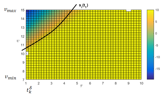
Figure 3: Illustration of the feasibility region for case 1.1.C.

V Design of the feasibility enforcement zone

Given all the information pertaining to CAVs $k$ and $i-1$, we can immediately determine the feasible region $\mathcal{F}_{i}$ for any CAV $i$ which may enter the CZ next. The role of the FEZ introduced prior to the CZ is to exert a control on $i$ that ensures its initial condition $(\tau,\upsilon)$ is such that $(\tau,\upsilon)\in\mathcal{F}_{i}$. Thus, while an optimal control is applied to $i$ within the CZ, the control used in the FEZ is not optimal, but it is necessary to guarantee that the subsequent optimal control is feasible. This is similar to controllers used at gateways of communication networks in order to “smooth” incoming traffic before applying optimal routing or scheduling policies on packets entering the network (in our case, CAVs entering a CZ).

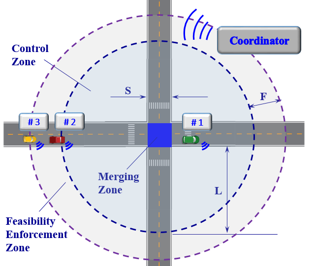
Figure 4: Intersection model with feasibility enforcement zone (FEZ) added.

The design of the FEZ rests on determining its length, denoted by $F_{i}$. Let $i$ denote a CAV entering the FEZ and let $k$ denote the CAV immediately preceding it. Let $v_{i}^{F}=v_{i}(t_{i}^{F})$ be the speed of $i$ upon entering the FEZ at time $t_{i}^{F}$ and let $u_{i}^{F}=u_{i}(t_{i}^{F})$ be the associated control (acceleration/deceleration). Then, assuming for simplicity that a fixed control $u_{i}^{F}$ is maintained throughout the FEZ, we have

$$F_{i}=\frac{\upsilon^{2}-(v_{i}^{F})^{2}}{2u_{i}^{F}},$$

where $\upsilon\equiv v_{i}^{0}$ is the speed of $i$ when it reaches the CZ after traveling a distance $F_{i}$. Clearly, the worst case in terms of the maximal value of $F_{i}$, denoted by $\bar{F}_{i}$, arises when $k$ enters the CZ at minimal speed $v_{min}$ and $v_{i}^{F}=$ $v_{max}$, in which case we must exert a minimal possible deceleration $u_{B}$, defined as a bound such that $u_{i,min}<u_{B}<0$. Therefore,

$$\bar{F}_{i}=\frac{\upsilon^{2}-v_{max}^{2}}{2u_{B}}>0.$$ (32)

On the other hand, recalling that $\tau=t_{i}^{0}$ is the time when $i$ reaches the CZ, the speed $\upsilon$ must also satisfy

$$\tau-t_{k}^{0}=\frac{\upsilon-v_{max}}{u_{B}}>0.$$ (33)

Thus, the length of the FEZ, $\bar{F}_{i}$, must be such that $(\tau,\upsilon)\in\mathcal{F}_{i}$ subject to (32)-(33). We show next that under a sufficient condition on the system parameters $v_{min}$, $v_{max}$, $u_{B}$, and $\delta$, there exists a value of $\bar{F}_{i}$ which guarantees that $(\tau,\upsilon)\in\mathcal{F}_{i}.$

Proposition 1

Suppose that

$$\frac{v_{min}-v_{max}}{u_{B}}\geqslant\frac{\delta}{v_{min}}$$ (34)

holds. Then, the following FEZ length guarantees that $(\tau,\upsilon)=(t_{k}^{0}+\frac{v_{min}-v_{max}}{u_{B}},v_{min})\in\mathcal{F}_{i}$:

$$\bar{F}=\frac{v_{min}^{2}-v_{max}^{2}}{2u_{B}}.$$ (35)

Proof: A necessary condition for the safety constraint (3) to be satisfied throughout the CZ is that $s_{i}(\tau)\geqslant\delta$. This is equivalent to $p_{k}(\tau)\geqslant\delta$, i.e., the distance traveled by $k$ by the time CAV $i$ enters the CZ must be no less that the safety lower bound $\delta$. The worst case arises when $v_{k}(t_{k}^{0})=v_{min}$ and remains constant at least through $[t_{k}^{0},\tau]$. This implies that

$$\tau-t_{k}^{0}\geqslant\frac{\delta}{v_{min}}.$$ (36)

Moreover, observe that an upper bound for $\bar{F}_{i}$ in (32), denoted by $\bar{F}$, occurs when $\upsilon=v_{min}$, so that (35) holds. Then, (33) and (36) imply (34). If this is satisfied, then $\tau=t_{k}^{0}+\frac{v_{min}-v_{max}}{u_{B}}$ is feasible, hence $(\tau,\upsilon)=(t_{k}^{0}+\frac{v_{min}-v_{max}}{u_{B}},v_{min})\in\mathcal{F}_{i}$. $\blacksquare$

Our analysis thus far has considered the case where the FEZ contains only CAV $i$ and its preceding CAV $k$. This allows us to specify the upper bound $\bar{F}$ in (35) for any such $i$. In general, however, there may already be multiple CAVs in the FEZ at the time that a new CAV enters it. We establish next that all such CAVs can be controlled to attain initial conditions in their respective feasibility regions.

Proposition 2

Let CAV $k$ enter the CZ when $N$ CAVs are in the preceding FEZ, ordered so that $k<k_{0}<k_{1}<\cdots<k_{N}$ with associated initial conditions when reaching the CZ $(\tau_{j},\upsilon_{j})$, $j=0,\ldots,N$. Assume that (34) holds and the FEZ length is given by (35). Then, $(\tau_{j},\upsilon_{j})\in\mathcal{F}_{j}$ for all $j=0,\ldots,N$.

Proof: From Proposition 1, setting $i=k_{0}$ we can attain $(\tau_{0},\upsilon_{0})\in\mathcal{F}_{0}$. It follows that all information related to $k_{0}$ is available to $k_{1}$ through the information set $Y_{k_{1}}(t)$ in (6). Next, setting $k=k_{0}$ and $i=k_{1}$, we can again apply Proposition 1 to attain $(\tau_{1},\upsilon_{1})\in\mathcal{F}_{1}$. This iterative process is repeated over all $j=0,\ldots,N$. $\blacksquare$

VI Simulation Examples

The effectiveness of the proposed FEZ and associated control is illustrated through simulation in MATLAB. For each direction, only one lane is considered. The parameters used are: $L=400$ m, $S=30$ m, $\delta=10$ m, $v_{max}=15$ m/s, $v_{min}=7$ m/s, $u_{i,max}=3$ m/s², $u_{i,min}=-5$ m/s² and $u_{B}=-2$ m/s², which satisfy condition (34). Based on (35), the length of the FEZ is set at $\bar{F}=44$ m. CAVs arrive at the FEZ based on a random arrival process and any speed within $[v_{min},v_{max}]$. Here, we assume a Poisson arrival process with rate $\lambda=1$ and the speeds are uniformly distributed over $[7,15]$.

We consider two cases: $(i)$ The FEZ is included preceding the CZ, and $(ii)$ No FEZ is included. The speed and position trajectories of the first 20 CAVs for the first case are shown in Fig. 5. In the position profiles, CAVs are separated into two groups: CAV positions shown above zero are driving from east to west or from west to east, and those below zero are driving from north to south or from south to north. These figures include different instances from each of Cases 1), 2), or 3) in Section III.A regarding the value of $t_{i}^{f}$. For example, CAV #2 is assigned $t_{2}^{f}=t_{1}^{f}$ and $v_{2}^{f}=v_{1}^{f}$, which corresponds to Case 1), whereas CAV #3 is assigned $t_{3}^{f}=t_{2}^{f}+\frac{S}{v_{3}^{f}}$ and $v_{3}^{f}=v_{2}^{f}$, which corresponds to Case 3) with $v_{i}(t_{i-1}^{f})=v_{i-1}(t_{i-1}^{f})$.

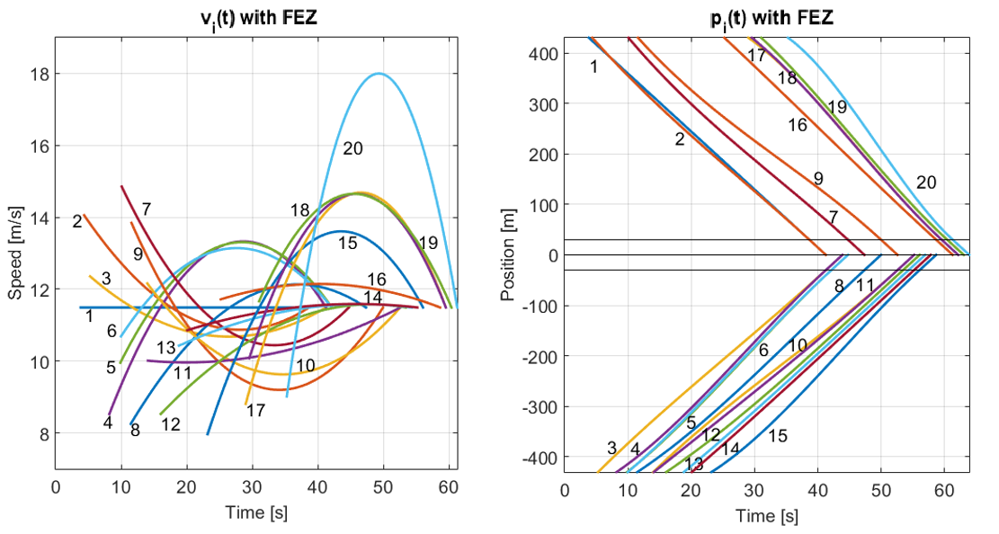
Figure 5: Speed $v_{i}(t)$ and position $p_{i}(t)$ trajectories of the first 20 CAVs.

To demonstrate the effectiveness of our feasibility enforcement control, we examine the distance $s_{i}(t)$ between two consecutive CAVs for the first 20 CAVs as shown in Fig. 6. In this example, each of CAVs #1, #2, #3 and #4 happens to be the first entering each of the four lanes respectively, hence all $s_{i}(t)$, $i=1,\ldots,4$, in (3) are undefined. Regarding the different $s_{i}^{\ast}(\tau,\upsilon)$ cases arising in Section IV, we observe that for CAV #11, $t_{11}^{\ast}=t_{11}^{0}$, which corresponds to Case 1; for CAV #16, $t_{16}^{\ast}=t_{2}^{m}$, which corresponds to Case 2; and for CAV #7, $t_{7}^{\ast}=t_{1}\in(t_{7}^{0},t_{1}^{m})$, which corresponds to Case 3. Without the FEZ (right side of Fig. 6), we can see that CAVs #5, #9, #10, #13, #14 and #19 all clearly violate the safety constraint (3), i.e., $s_{i}(t)<\delta=10$ for at least some $t\in[t_{i}^{0},t_{i}^{m}]$. With the FEZ included, these CAVs are capable of adjusting their speed and CZ entry time to some feasible initial conditions and they all satisfy the safety constraint, as clearly seen on the left side of Fig. 6. On the other hand, given that CAV #16 is on the same lane as CAV #2 and that CAV #2 is the first one in that lane, there is no need for #16 to make any adjustment since it already has feasible initial conditions with respect to the optimal control problem solved within the CZ.

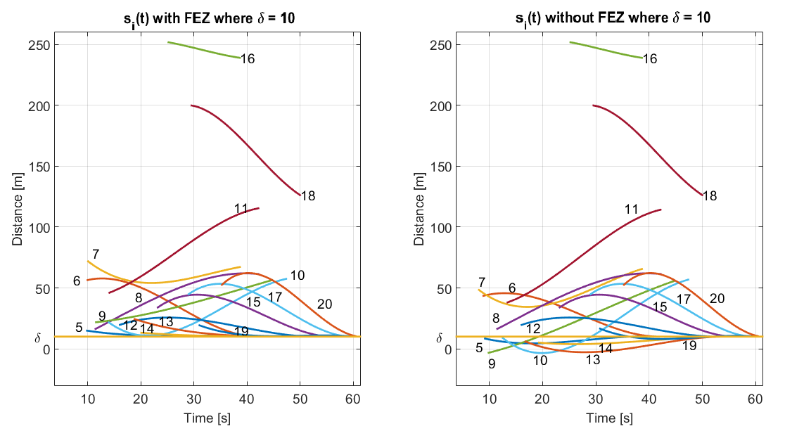
Figure 6: Distance $s_{i}(t)$ trajectories of the first 20 CAVs.

VII Conclusion

Earlier work [14] has established a decentralized optimal control framework applied for coordinating online a continuous flow of CAVs crossing two adjacent intersections in an urban area. However, the feasibility of the optimal control solution  depends on the initial conditions of each CAV as it enters the “control zone” (CZ) of each intersection. We have shown that there exists a feasibility region for each CAV in the space defined by its arrival time and speed and this can be fully characterized in terms of information known to CAV $i$ before it enters the CZ, which can be enforced through a properly designed “feasibility enforcement zone” (FEZ) that precedes the CZ. Ensuring that optimal control solutions are feasible paves the way for exploring more efficient event-driven solutions, allow for different classes of CAVs with distinct physical characteristics, and for alternative problem formulations that exploit a potential trade-off between fuel consumption and congestion.

References

- [1] L. Li, D. Wen, and D. Yao, “A Survey of Traffic Control With Vehicular Communications,” IEEE Transactions on Intelligent Transportation Systems, vol. 15, no. 1, pp. 425–432, 2014.
- [2] J. L. Fleck, C. G. Cassandras, and Y. Geng, “Adaptive quasi-dynamic traffic light control,” IEEE Transactions on Control Systems Technology, 2015, DOI: 10.1109/TCST.2015.2468181, to appear.
- [3] K. Dresner and P. Stone, “Multiagent traffic management: a reservation-based intersection control mechanism,” in Proceedings of the Third International Joint Conference on Autonomous Agents and Multiagents Systems, 2004, pp. 530–537.
- [4] ——, “A Multiagent Approach to Autonomous Intersection Management,” Journal of Artificial Intelligence Research, vol. 31, pp. 591–653, 2008.
- [5] A. de La Fortelle, “Analysis of reservation algorithms for cooperative planning at intersections,” 13th International IEEE Conference on Intelligent Transportation Systems, pp. 445–449, Sept. 2010.
- [6] S. Huang, A. Sadek, and Y. Zhao, “Assessing the Mobility and Environmental Benefits of Reservation-Based Intelligent Intersections Using an Integrated Simulator,” IEEE Transactions on Intelligent Transportation Systems, vol. 13, no. 3, pp. 1201,1214, 2012.
- [7] L. Li and F.-Y. Wang, “Cooperative Driving at Blind Crossings Using Intervehicle Communication,” IEEE Transactions in Vehicular Technology, vol. 55, no. 6, pp. 1712,1724, 2006.
- [8] F. Yan, M. Dridi, and A. El Moudni, “Autonomous vehicle sequencing algorithm at isolated intersections,” 2009 12th International IEEE Conference on Intelligent Transportation Systems, pp. 1–6, 2009.
- [9] I. H. Zohdy, R. K. Kamalanathsharma, and H. Rakha, “Intersection management for autonomous vehicles using iCACC,” 2012 15th International IEEE Conference on Intelligent Transportation Systems, pp. 1109–1114, 2012.
- [10] F. Zhu and S. V. Ukkusuri, “A linear programming formulation for autonomous intersection control within a dynamic traffic assignment and connected vehicle environment,” Transportation Research Part C: Emerging Technologies, 2015.
- [11] J. Lee and B. Park, “Development and Evaluation of a Cooperative Vehicle Intersection Control Algorithm Under the Connected Vehicles Environment,” IEEE Transactions on Intelligent Transportation Systems, vol. 13, no. 1, pp. 81–90, 2012.
- [12] D. Miculescu and S. Karaman, “Polling-Systems-Based Control of High-Performance Provably-Safe Autonomous Intersections,” in 53rd IEEE Conference on Decision and Control, 2014.
- [13] J. Rios-Torres and A. A. Malikopoulos, “A Survey on the Coordination of Connected and Automated Vehicles at Intersections and Merging at Highway On-Ramps,” IEEE Transactions on Intelligent Transportation Systems, 2016 (forthcoming).
- [14] Y. Zhang, A. A. Malikopoulos, and C. G. Cassandras, “Optimal control and coordination of connected and automated vehicles at urban traffic intersections,” in Proceedings of the American Control Conference, 2016, pp. 6227–6232.
- [15] A. A. Malikopoulos, C. G. Cassandras, and Y. Zhang, “A decentralized optimal control framework for connected automated vehicles at urban intersections,” arXiv:1602.03786, 2016.
- [16] J. Rios-Torres, A. A. Malikopoulos, and P. Pisu, “Online Optimal Control of Connected Vehicles for Efficient Traffic Flow at Merging Roads,” in 2015 IEEE 18th International Conference on Intelligent Transportation Systems, Canary Islands, Spain, September 15-18, 2015.
- [17] J. Rios-Torres and A. A. Malikopoulos, “Automated and Cooperative Vehicle Merging at Highway On-Ramps,” IEEE Transactions on Intelligent Transportation Systems, 2016 (forthcoming).
- [18] M. Zhong and C. G. Cassandras, “Asynchronous distributed optimization with event-driven communication,” IEEE Transactions on Automatic Control, vol. 55, no. 12, pp. 2735–2750, 2010.