Ptolemy Constants as Described by Eccentricity

Abstract

Let $J$ denote a simple closed curve in the plane.  Let points $a$, $b$, $c$, $d\in J$ occur in this order when traversing $J$ in a counterclockwise direction.  Define $p(a,b,c,d)$ to be the ratio of $ab\cdot cd+ad\cdot bc$ to $ac\cdot bd$, where $zw$ denotes distance between $z$ and $w$.  Define $P(J)$ to be the supremum of $p$ over all such points.  Harmaala & Klén [1] provided bounds on $P(J)$ when $J$ is an ellipse or rectangle of eccentricity $\varepsilon$.  We nonrigorously give formulas for $P(J)$ here, in the hope that someone else can fill gaps in our reasoning.

Given parameters $0\leq\theta_{1}<$ $\theta_{2}<\theta_{3}<\theta_{4}<2\pi$ and $0\leq\varepsilon<1$, consider vertices

$$\begin{array}[c]{ccc}v_{k}=\left(\cos\theta_{k},\sqrt{1-\varepsilon^{2}}\,\sin\theta_{k}\right),&&1\leq k\leq 4\end{array}$$

of a convex quadrilateral inscribed within the planar ellipse

$$\begin{array}[c]{ccc}x^{2}+\dfrac{y^{2}}{1-\varepsilon^{2}}=1&&\text{(with foci at }(\pm\varepsilon,0)\text{).}\end{array}$$

The ratio

$$p=\frac{\left|v_{1}-v_{2}\right|\cdot\left|v_{3}-v_{4}\right|+\left|v_{1}-v_{4}\right|\cdot\left|v_{2}-v_{3}\right|}{\left|v_{1}-v_{3}\right|\cdot\left|v_{2}-v_{4}\right|}$$

involves lengths of sides in the numerator and lengths of diagonals in the denominator.  Let $P(\varepsilon)$ denote the supremum of the ratio over all parameters $\theta_{1}$, $\theta_{2}$, $\theta_{3}$, $\theta_{4}$.  It is thought that $P(\varepsilon)$ measures the “roundness of planar curves”.  Harmaala & Klén [1] proved that

$$\frac{1}{2}\left(\frac{1}{\sqrt{1-\varepsilon^{2}}}+\frac{\sqrt{1-\varepsilon^{2}}}{1}\right)\leq P(\varepsilon)\leq\csc\left(\frac{\pi\sqrt{1-\varepsilon^{2}}}{2}\right)$$

but evidently did not tighten these bounds.

Symbolic calculations of the gradient vector and Hessian matrix of $p$ indicate that

$$(\theta_{1},\theta_{2},\theta_{3},\theta_{4})=\left(0,\frac{\pi}{2},\pi,\frac{3\pi}{2}\right)$$

corresponds to a local maximum of $p$, regardless of the value of $\varepsilon$.  For example, the Hessian matrix at this point is

$$\frac{-\varepsilon^{4}}{8\sqrt{1-\varepsilon^{2}}}\left(\begin{array}[c]{cccc}\dfrac{3-\varepsilon^{2}}{2-\varepsilon^{2}}&0&\dfrac{1-\varepsilon^{2}}{2-\varepsilon^{2}}&0\\ 0&\dfrac{3-2\varepsilon^{2}}{\left(2-\varepsilon^{2}\right)\left(1-\varepsilon^{2}\right)}&0&\dfrac{1}{\left(2-\varepsilon^{2}\right)\left(1-\varepsilon^{2}\right)}\\ \dfrac{1-\varepsilon^{2}}{2-\varepsilon^{2}}&0&\dfrac{3-\varepsilon^{2}}{2-\varepsilon^{2}}&0\\ 0&\dfrac{1}{\left(2-\varepsilon^{2}\right)\left(1-\varepsilon^{2}\right)}&0&\dfrac{3-2\varepsilon^{2}}{\left(2-\varepsilon^{2}\right)\left(1-\varepsilon^{2}\right)}\end{array}\right)$$

and all conditions of the multivariate second derivative test are clearly met.  Numerical optimization techniques suggest that this, in fact, corresponds to a global maximum.  We do not see how to verify this rigorously.  If an analytical workaround could somehow be discovered, we would have

$$P(\varepsilon)=\dfrac{2-\varepsilon^{2}}{2\sqrt{1-\varepsilon^{2}}}$$

for an ellipse of eccentricity $\varepsilon$, which is the lower bound given in [1], Theorem 1.7.

Consider instead vertices $v_{1}$, $v_{2}$, $v_{3}$, $v_{4}$ of a convex quadrilateral inscribed within the planar rectangle

$$\max\left\{\left|x\right|,\frac{\left|y\right|}{\sqrt{1-\varepsilon^{2}}}\right\}=1.$$

Cyclicity is assumed as before.  This is analogous to the ellipse, although the existence of sharp corners changes the nature of the analysis.  Here we have

$$P(\varepsilon)=\left\{\begin{array}[c]{lll}\sqrt{2}&&\text{if }0\leq\varepsilon\leq\sqrt{3}/2,\\ \dfrac{\sqrt{1+4\left(1-\varepsilon^{2}\right)}}{2\sqrt{1-\varepsilon^{2}}}&&\text{if }\sqrt{3}/2<\varepsilon<1\end{array}\right.$$

for a rectangle of eccentricity $\varepsilon$, which again is the lower bound given in [1], Corollary 4.8.  The threshold $\varepsilon=\sqrt{3}/2$ implies $\sqrt{1-\varepsilon^{2}}=1/2$, that is, a transition occurs at a $2\times 1$ rectangle.

The left-hand rectangle in Figure 1 shows an optimizing vertex configuration for $0\leq\varepsilon\leq\sqrt{3}/2$; the right-hand rectangle shows an optimizing vertex configuration for $\sqrt{3}/2\leq\varepsilon<1$.  For the former,

$$\begin{array}[c]{lll}v_{1}=\left(1,\sqrt{1-\varepsilon^{2}}\right),&&v_{2}=\left(-1,\delta-\sqrt{1-\varepsilon^{2}}\right),\\ v_{3}=\left(-1,-\sqrt{1-\varepsilon^{2}}\right),&&v_{4}=\left(\delta-1,-\sqrt{1-\varepsilon^{2}}\right)\end{array}$$

give

$$\frac{\sqrt{4+\left(\delta-2\sqrt{1-\varepsilon^{2}}\right)^{2}}\cdot\delta+\sqrt{\left(\delta-2\right)^{2}+4\left(1-\varepsilon^{2}\right)}\cdot\delta}{\sqrt{4+4\left(1-\varepsilon^{2}\right)}\cdot\sqrt{2}\,\delta}\rightarrow\sqrt{2}$$

as $\delta\rightarrow 0^{+}$.  For the latter,

$$\begin{array}[c]{lll}v_{1}=\left(0,\sqrt{1-\varepsilon^{2}}\right),&&v_{2}=\left(-1,-\sqrt{1-\varepsilon^{2}}\right),\\ v_{3}=\left(0,-\sqrt{1-\varepsilon^{2}}\right),&&v_{4}=\left(1,-\sqrt{1-\varepsilon^{2}}\right)\end{array}$$

and the rest follows trivially.  A sizeable variety of vertex configurations need to be ruled out in order to verify global maximality.

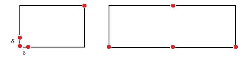
Figure 1: On the left are rectangles that are $2\times 1$ or less eccentric.  On the right are rectangles that are $2\times 1$ or more eccentric.

Ptolemy constants remain open for a regular hexagon and for a Reuleaux triangle, as well as for arbitrary convex quadrilaterals.  Discovering these could be a fruitful exercise in computer algebra.

References

• [1] E. Harmaala andΒ R. KlΓ©n, Ptolemy constant and uniformity, arXiv:1604.05367.
Steven Finch
Dept. of Statistics
Harvard University
Cambridge, MA, USA
steven_finch@harvard.edu