Robust benchmarking in noisy environments
Abstract
We propose a benchmarking strategy that is robust in the presence of timer error, OS jitter and other environmental fluctuations, and is insensitive to the highly nonideal statistics produced by timing measurements. We construct a model that explains how these strongly nonideal statistics can arise from environmental fluctuations, and also justifies our proposed strategy. We implement this strategy in the BenchmarkTools Julia package, where it is used in production continuous integration (CI) pipelines for developing the Julia language and its ecosystem.
I Introduction
Authors of high performance applications rely on benchmark suites to detect and avoid program regressions. However, many developers often run benchmarks and interpret their results in an ad hoc manner with little statistical rigor. This ad hoc interpretation wastes development time and can lead to misguided decisions that worsen performance.
In this paper, we consider the problem of designing a language- and platform-agnostic benchmarking methodology that is suitable for continuous integration (CI) pipelines and manual user workflows. Our methodology especially focuses on the accommodation of benchmarks whose expected executions times are short enough that timing measurements are vulnerable to error due to insufficient system timer accuracy (generally on the order of microseconds or shorter).
I-A Accounting for performance variations
Modern hardware and operating systems introduce many confounding factors that complicate a developer’s ability to reason about variations in user space application performance [1].111A summary of these factors can be found in the BenchmarkTools documentation in the docs/linuxtips.md file. Consecutive timing measurements can fluctuate, possibly in a correlated manner, in ways which depend on a myriad of factors such as environment temperature, workload, power availability, and network traffic, and operating system (OS) configuration.
There is a large body of research on system quiescence aiming to identify and control for individual sources of variation in program run time measurements, each of which must be ameliorated in its own way. Many factors stem from OS behavior, including CPU frequency scaling [2], address space layout randomization (ASLR) [3], virtual memory management [4, 5], differences between CPU privilege levels [6], context switches due to interrupt handling [7], activity from system daemons and cluster managers [8], and suboptimal process- and thread-level scheduling [9]. Even seemingly irrelevant configuration parameters like the size of the OS environment can confound experimental reproducibility by altering the alignment of data in memory [10]. Other sources of variation come from specific language features or implementation details. For example, linkers for many languages are free to choose the binary layout of the library or executable arbitrarily, resulting in non-deterministic memory layouts [11]. This problem is exacerbated in languages like C++, whose compilers introduce arbitrary name mangling of symbols [12]. Overzealous compiler optimizations can also adversely affect the accuracy of hardware counters [6], or in extreme cases eliminate key parts of the benchmark as dead code. Yet another example is garbage collector performance, which is influenced from system parameters such as heap size [13].
I-B Statistics of timing measurements are not i.i.d.
The existence of many sources of performance variation result in timing measurements that are not necessarily independent and identically distributed (i.i.d.). As a result, many textbook statistical approaches fail due to reliance on the central limit theorem, which does not generally hold in the non-i.i.d. regime. In particular, empirical program timing distributions are also often heavy-tailed, and hence contain many outliers that distort measures of central tendency like the mean, and are not captured in others like the median.
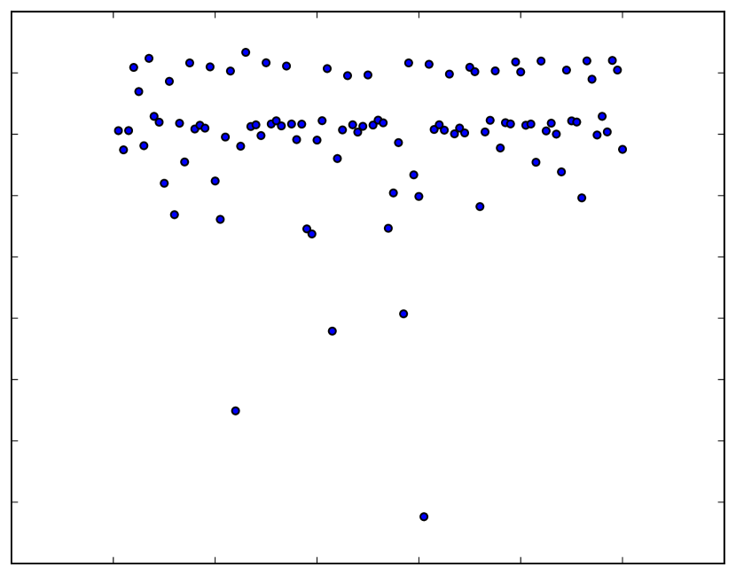
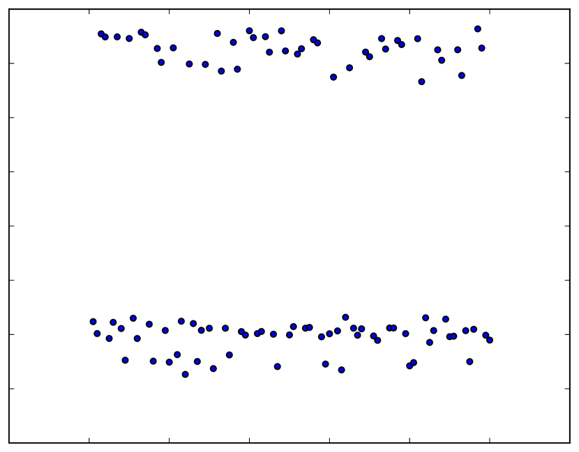
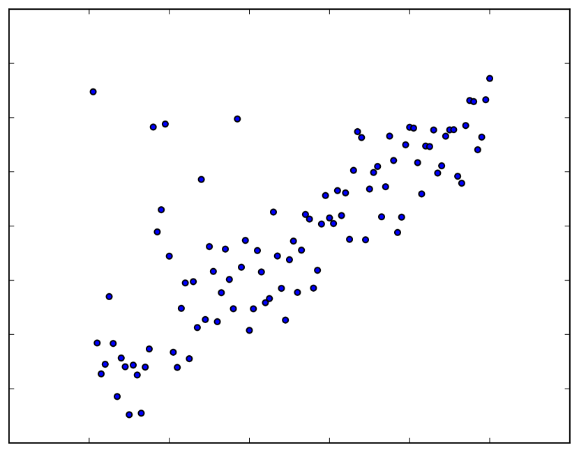
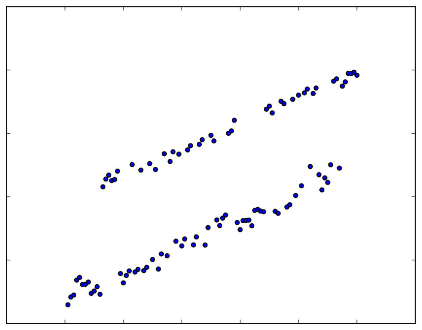
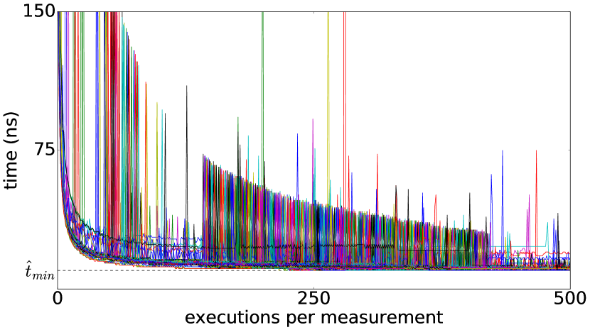
The violation of the central limit theorem can be seen empirically in many Julia benchmarks. For example, Figure 1 shows that none of the four illustrative benchmarks considered in this paper exhibit normality in the sample mean. Instead, we see that the mean demonstrates skewed density and outliers in the first benchmark, bimodality in the second and fourth benchmarks, and upward drift in the third and fourth benchmarks.
Many other authors have also noted the lack of textbook statistical behavior in timing measurements [14, 15, 16, 17]. Authors have also noted the poor stastistical power of standard techniques such as -tests or Student t-tests for benchmark timings [18, 10, 19, 15, 17]. Parametric outlier detection techniques, such as the 3-sigma rule used in benchmarking software like AndroBench[20], can also fail when applied to non-i.i.d. timing measurements.
There is a lack of consensus over how non-ideal timing measurements should be treated. Some authors propose automated outlier removal and analyzing the remaining bulk distribution [20]; however, these methods run the risk of fundamentally distorting the true empirical distribution for the sake of normal analysis. Other authors have proposed purposely introducing randomness in the form of custom OS kernels [21, 22], custom compilers providing reproducible [11] or consistently randomized [23] binary layouts, or low-variability garbage collectors [24]. Unfortunately, these methods are specific to a single programming language, implementation, and/or platform. Furthermore, these methods often require administrative privileges and drastic modifications to the benchmarking environment, which are impractical to demand from ordinary users.
I-C Existing benchmarking methodologies
While it is impossible to eliminate performance variation entirely [25, 17], benchmarking methodologies that attempt to account for both measurement error and external sources of variation do exist. For example, the Haskell microbenchmarking package criterion [26] attempts to thwart error due to timer inaccuracy by growing the number of benchmark executions per timing measurement as more timing measurements are obtained. After all measurements are taken, a summary estimate of the benchmark run time is obtained by examining the derivative of the ordinary least squares regression line at the point of a single evaluation point. There are three disadvantages to this approach. First, the least squares fit is sensitive to outliers [27] (though criterion does warn the user if outliers are detected). Second, measurements made earlier in this experiment are highly vulnerable to timer error, since few benchmark repetitions are used. These early measurements can skew the regression, and hence also skew the final run time estimate. Third, measurements made later in the experiment can repeat the benchmark more times than are necessary to overcome timer error, constituting an inefficient use of experiment time.
Another approach focuses on eliminating “warm-up”, assuming that first few runs of a benchmark are dominated by transient background events that eventually vanish and the timing measurements eventually become i.i.d. [19]. Their approach is largely platform-agnostic, recognizes the pitfalls of inter-measurement correlations, and acknowledges that merely increasing the number of benchmark repetitions is not always a sufficient strategy to yield i.i.d. samples. However, the assumption (based on common folklore) that benchmarks exhibit warm-up is often false, as is clear from Fig. 1 and elsewhere [17]: even Ref. [19] itself resorts to ad hoc judgment to work around the lack of a distinct warm-up phase. There is also no reason to believe that even if warm-up were observed, that the post-warm-up timings will be i.i.d. Furthermore, the authors do not report if their statistical tools generate correct confidence intervals. The moment-corrected formulae described are accurate only for near-normal distributions, which is unlikely to hold for the kinds of distributions we observed in real world statistics. Additionally, the methodology requires a manual calibration experiment to be run for each benchmark, compiler, and platform combination. As a result, this method is is difficult to automate on the scale of Julia’s standard library benchmark suite, which contains over 1300 benchmarks, and is frequently expanded to improve performance test coverage.
Below, we describe our methodology to benchmarking for detecting performance regressions, and how it is justified from a microscopic model for variations in timing measurements. To the best of our knowledge, our work is the first benchmarking methodology that can be fully automated, is robust in its assumption of non-i.i.d. timing measurement statistics, and makes efficient use of a limited time budget.
II Terms and definitions
-
•
, , , and denote benchmarkable programs, each defined by a tape (sequence) of instructions.
-
•
is the instruction in the tape defining program . Instructions are indexed in bracketed superscripts, .
-
•
is the delay instruction associated with . Delay instructions are defined in Sec. III.
-
•
is a timing measurement, namely the amount of time taken to perform executions of a benchmarkable program. This quantity is directly measurable in an experiment.
-
•
is a theoretical execution time. is the minimum time required to perform a single execution of on a given computer.
-
•
Estimated quantities are denoted with a hat, . For example, is an estimate of the theoretical execution time .
-
•
A benchmark experiment is a recipe for obtaining multiple timing measurements for a benchmarkable program. Experiments can be executed to obtain trials. The trial of an experiment is a collection of timing measurements . Trial indices are always written using embraced superscripts, .
-
•
denotes time quantities that are external to the benchmarkable program:
-
–
is the time budget for an experiment.
-
–
is the accuracy of the system timer, i.e. an upper bound on the maximal error in using the system timer to time an experiment.
-
–
is the precision of the system timer, namely the smallest nonzero time interval measurable by the timer.
-
–
-
•
is the time delay due to the delay factor for delay instruction . Specifically, is the factor’s time scale and is the factor’s trigger coefficient, as introduced Sec. III. Delay factors are indexed with parenthesized superscripts, .
-
•
is the measurement error due to timer inaccuracy.
-
•
is the total contribution of all delay factors found in measurement , plus the measurement error .
-
•
is the total trigger count of the delay factor during the execution of program .
-
•
is an oracle function that, when evaluated at an execution time , estimates an appropriate necessary to overcome measurement error due to and . The oracle function is described in detail in Sec. IV-C.
III A model for benchmark timing distributions
We now present a statistical description of how benchmark programs behave when they are run in serial. Our model deliberately avoids the problematic assumption that timing measurments are i.i.d. We will use this model later to justify the design of a new automated experimental procedure.
III-A User benchmarks run with uncontrollable delays
Let be a deterministic benchmark program which consists of an instruction tape consisting of instructions:
| (1) |
Let be the run time of instruction . Then, the total run time of can be written .
While a computer may be directed to execute , it may not necessarily run the program’s instructions as they are originally provided, since the environment in which runs is vulnerable to the factors described earlier in Sec. I-A. Crucially, these factors only delay the completion of the original instructions, rather than speed them up.222While there are a very few external factors which might speed up program execution, such as frequency scaling [2], they can be easily accounted for by ensuring that power consumption profiles are always set for maximal performance. We therefore assume that these factors have been accounted for. Therefore, we call them delay factors; they can be modeled as extra instructions which, when interleaved with the original instructions, do not change the semantics of , but still add to the program’s total run time. Thus, we can define a new program which consists of ’s original instructions interleaved with additional delay instructions :
| (2) |
The run time of can then be written
| (3) |
where is the execution time of . Since , it follows that .
The run time of each delay instruction, , can be further decomposed into the runtime contributions of individual delay factors. Let us imagine that each delay factor can either contribute or not contribute to . Assuming that each delay factor triggers inside with constant probability of taking a fixed time , we can then write:
| (4) |
where is a Bernoulli random variable with success probability . We denote the total number of times the delay factor was triggered during the execution of as the trigger count . Since the trigger count is a sum of independent Bernoulli random variables with nonidentical success probabilities, is itself a random variable that follows a Poisson binomial distribution parameterized by the success probabilities . Our final expression for in terms of these quantities is then:
| (5) |
In summary, our model treats as a random variable whose distribution depends on the trigger probabilities , which are determined by the combined behavior of the delay factors and the initial benchmark program .
III-B Repeated benchmark execution is often necessary but not always sufficient
As mentioned in Sec. I-C, experiments which measure program performance usually incorporate multiple benchmark executions to obtain more accurate measurements. We now apply our model to show that multiple executions are necessary to eliminate error due to timer inaccuracy, but are insufficient to obviate delay factors.
Represent executions of the program comprised of instructions as a single execution of a program , which is the result of concatenating copies of :
| (6) |
with for . The subscripts on denote the program which contains that instruction, with the 0 subsubscript dropped for brevity.
Now interleave delay instructions as before to obtain the program that is actually executed. is not simply repetitions of , since the delay instructions in are not simply copies of the delay instructions in . An observed timing measurement of a single execution of can be decomposed as:
| (7) |
where is the error due to timer inaccuracy (whose magnitude must by definition be smaller than ).
We may try to determine from the experimental time as , which is also the gradient of a linear model for against when the intercept is zero. However, our model gives instead:
| (8) |
All the terms on the right hand side other than constitute the error in our measurement. For large , the term arising from timer inaccuracy becomes negligible, but the behavior of the other term depends on the specific structure of the delay factors. In the best case, each delay factor triggers times, so that as desired. However, in the worst case, every factor triggers on every instruction, , and the large behavior of does not reduce to the true run time , but rather:
| (9) |
(9) is a key result of our model: one cannot always reliably eliminate bias due to external variations simply by executing the benchmark many times. Whether or not increasing can render the delay factor term negligible depends entirely on the distribution of trigger counts , which are difficult or impossible to control (see Sec. I-A). Therefore, we can only expect that at large gives us at best an overestimate of the true run time .
IV An automated procedure for configuring performance experiments
In this section, we present an experimental procedure for automatically selecting useful values of for a given benchmark program, which can be justified from our model of serial benchmark execution above. Our procedure estimates a value for which primarily minimizes error in timing measurements and secondarily maximizes the number of measurements obtainable within a given time budget.
IV-A An algorithm for estimating the optimal value
Given and a total time budget , we use the automatable procedure in Alg. 1 for guessing the minimum value of required to amortize measurement error due to timer inaccuracy. The algorithm makes use of an oracle function , which is discussed in greater detail below in Sec. IV-C.
The upper bound in Alg. 1 is the ratio of timer accuracy to timer precision. If each timing measurement consists of more than repetitions, then the contribution of timer inaccuracy to the total error is less than , and so is too small to measure. Thus, there is no reason to pick . In practice, need only be an overestimate for the timer accuracy, which would raise the determined, but is still an acceptable result.
Alg. 1 need only be applied once per benchmark, since the estimated can be cached for use in subsequent experiments on the same machine. Thus, we consider this algorithm an automated preprocessing step that does not count against our time budget . In this regard, our approach differs significantly from other approaches like criterion, which re-determines every time a benchmark is run.
IV-B Justifying the minimum estimator
We will now justify Alg. 1’s use of the minimum to estimate , as opposed to the more common median or mean. Consider the total error term for a given timing measurement , such that . The minimum estimator applied to our timing measurements can then be written as:
| (10) |
Thus, is the estimate of which minimizes the error terms appearing in our sample.
In the limit where the delay factor time scales are greater than , the total error terms will always be positive, such that choosing the smallest timing measurement will choose the sample with the smallest magnitude of error. If the delay factor time scales are less than , choosing the smallest timing measurement might choose a sample which underestimates due to negative timer error. In this case, Alg. 1 will simply pick a larger than is strictly necessary, which is still acceptable.
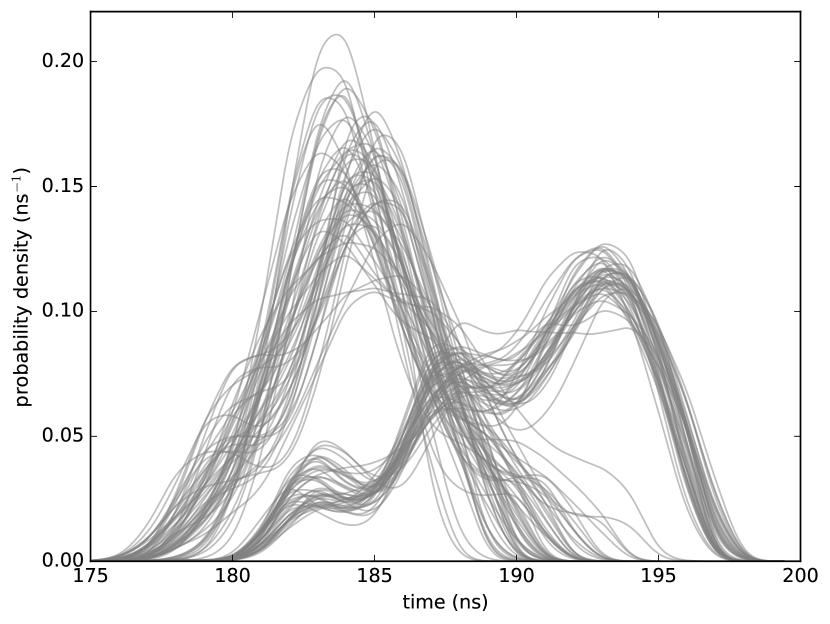
Figs. 3 and 4 provide further justification for the minimum over other common estimators like the median, mean, or trimmed mean. Recall from Section III that the error terms are sampled from a sum of scaled random variables following nonidentical Poisson binomial distributions. As such, these terms can and do exhibit multimodal behavior. While estimators like the median and trimmed mean are known to be robust to outliers [27], Fig. 3 demonstrates that they still capture bimodality of the distributions plotted in Fig. 4. Thus, these estimators are undesirable for choosing , since the result could vary drastically between different executions of Alg. 1, depending on which of the estimator’s modes was captured in the sample, and hence affect reproducibility. In contrast, the distribution of the minimum across all experimental trials is unimodal in all cases we have observed. Thus for our purposes, the minimum is a unimodal, robust estimator for the location parameter of a given benchmark’s timing distribution.
IV-C The oracle function
Our heuristic takes as input an oracle function that maps expected run times to an optimal number of executions per measurement. While Alg. 1 does not directly describe , appropriate choices for this function should have the following properties:
-
•
has a discrete range .
-
•
is monotonically decreasing, so that the longer the run time, the fewer repetitions per measurement.
-
•
, so that there is only weak dependence on the timer precision parameter, which may not be accurately known.
-
•
, so that there is only weak dependence on the timer accuracy parameter, which may not be accurately known.
-
•
, so that benchmarks that take a short time to run are not repeated more times than necessary to mitigate timer inaccuracy.
-
•
, so that benchmarks that take a long time to run need not be repeated.
There are many functions that satisfy these criteria. One useful example takes the form of the generalized logistic function:
| (11) |
where reasonable values of and are approximately and .
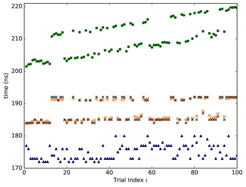
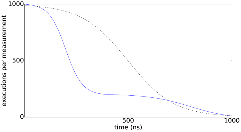
In practice, we have found that better results can be achieved by first approximating with a lookup table, then modifying the lookup table based on empirical observations. This was accomplished by examining many benchmarks with a variety of known run times at different time scales, seeking for each run time the smallest value at which the minimum estimate appears to converge to a lower bound (e.g. around for the benchmark in Fig. 2). Fig. 5 plots both (11) and an empirically obtained lookup table as potential oracle functions.
V Implementation in Julia
The experimental methodology in this paper is implemented in the BenchmarkTools Julia package333https://github.com/JuliaCI/BenchmarkTools.jl. In addition to the BaseBenchmarks444https://github.com/JuliaCI/BaseBenchmarks.jl and Nanosoldier555https://github.com/JuliaCI/Nanosoldier.jl packages, the BenchmarkTools package implements the on-demand CI benchmarking service used by core Julia developers to compare the performance of proposed language changes with respect to over 1300 benchmarks. Since this CI benchmarking service began in early 2016, it has caught and prevented the introduction of dozens of serious performance regressions into Julia’s standard library (defining a serious regression as a or greater increase in a benchmark’s minimum execution time).
The benchmarks referenced in this paper are Julia benchmarks written and executed using BenchmarkTools. A brief description of each benchmark is offered below:
-
•
The sumindex(a, inds) benchmark sums over all a[i] for all i in inds. This test stresses memory layout via element retrieval.
-
•
The pushall!(a, b) benchmark pushes elements from b into a one by one, additionally generating a random number at each iteration (the random number does not affect the output). This test stresses both random number generation and periodic reallocation that occurs as part of Julia’s dynamic array resizing algorithm.
-
•
The branchsum(n) benchmark loops from 1 to n. If the loop variable is even, a counter is decremented. Otherwise, an inner loop is triggered which runs from 1 to n, in which another parity test is performed on the inner loop variable to determine whether to increment or decrement the counter. This test stresses periodically costly branching within loop iterations.
-
•
The manyallocs(n) allocates an array of n elements, where each element is itself an array. The inner array length is determined by a random number from 1 to n, which is regenerated when each new array is constructed. However, the random number generator is reseeded before each generation so that the program is deterministic. This test stresses random number generation and the frequent allocation of arrays of differing length.
The mock benchmark suite referenced in this paper is hosted on GitHub at https://github.com/jiahao/paper-benchmark.
VI Conclusion
The complexities of modern hardware and software environments produce variations in benchmark timings, with highly nonideal statistics that complicate the detection of performance regressions. Timing measurements taken from real Julia benchmarks confirm the observations of many other authors showing highly nonideal, even multimodal behavior, exhibited by even the simplest benchmark codes.
Virtually all timing variations are delays caused by flushing cache lines, task switching to background OS processes, or similar events. The simple observation that variations never reduce the run time led us to consider a straightforward analysis based on a simple model for delays in a serial instruction pipeline. Our results suggest that using the minimum estimator for the true run time of a benchmark, rather than the mean or median, is robust to nonideal statistics and also provides the smallest error. Our model also revealed some behaviors that challenge conventional wisdom: simply running a benchmark for longer, or repeating its execution many times, can render the effects of external variation negligible, even as the error due to timer inaccuracy is amortized.
Alg. 1 presents an automatable heuristic for selecting the minimum number of executions of a benchmark per measurement required to defeat timer error. This strategy has been implemented in the BenchmarkTools Julia package, which is employed daily and on demand as part Julia’s continuous integration (CI) pipeline to evaluate the performance effects of proposed changes to Julia’s standard library in a fully automatic fashion. BenchmarkTools can also be used to test the performance of user-authored Julia packages.
Acknowledgment
We thank the many Julia developers, in particular Andreas Noack (MIT), Steven G. Johnson (MIT) and John M. White (Facebook), for many insightful discussions.
This research was supported in part by the U.S. Army Research Office under contract W911NF-13-D-0001, the Intel Science and Technology Center for Big Data, and DARPA XDATA.
References
- [1] J. L. Hennessy and D. A. Patterson, Computer Architecture: A Quantitative Approach, 5th ed., ser. The Morgan Kaufmann Series in Computer Architecture and Design. San Francisco, CA: Morgan Kaufmann, 2011.
- [2] Red Hat Enterprise Linux 6 Performance Tuning Guide, Red Hat, Inc, 2016.
- [3] H. Shacham, M. Page, B. Pfaff, E.-J. Goh, N. Modadugu, and D. Boneh, “On the effectiveness of address-space randomization,” in CCS ’04 Proceedings of the 11th ACM Conference on Computer and Communications Security. New York: ACM, 2004, pp. 298–307.
- [4] Y. Oyama, S. Ishiguro, J. Murakami, S. Sasaki, R. Matsumiya, and O. Tatabe, “Reduction of operating system jitter caused by page reclaim,” in ROSS ’14 Proceedings of the 4th International Workshop on Runtime and Operating Systems for Supercomputers, no. 9. New York: ACM, 2014.
- [5] ——, “Experimental analysis of operating system jitter caused by page reclaim,” The Journal of Supercomputing, vol. 72, no. 5, pp. 1946–1972, may 2016.
- [6] D. Zaparanuks, M. Jovic, and M. Hauswirth, “Accuracy of performance counter measurements,” in ISPASS 2009. IEEE International Symposium on Performance Analysis of Systems and Software, 2009, pp. 23–32.
- [7] D. Tsafrir, “The context-switch overhead inflicted by hardware interrupts (and the enigma of do-nothing loops),” in ExpCS ’07 Proceedings of the 2007 Workshop on Experimental Computer Science, no. 4. New York: ACM, 2007.
- [8] F. Petrini, D. J. Kerbyson, and S. Pakin, “The case of the missing supercomputer performance: Achieving optimal performance on the 8,192 processors of ASCI Q,” in SC’03 Proceedings of the ACM/IEEE Conference on Supercomputing. IEEE, 2003, pp. 55–71.
- [9] J.-P. Lozi, B. Lepers, J. Funston, F. Gaud, V. Quéma, and A. Fedorova., “The Linux scheduler: a decade of wasted cores,” in To appear in EuroSys ’16 Proceedings of the Eleventh European Conference on Computer Systems. New York: ACM, 2016.
- [10] T. Mytkowicz, A. Diwan, M. Hauswirth, and P. F. Sweeney, “Producing wrong data without doing anything obviously wrong!” in ASPLOS XIV Proceedings of the 14th international conference on Architectural support for programming languages and operating systems. New York: ACM, 2009, pp. 265–276.
- [11] A. Georges, L. Eeckhout, and D. Buytaert, “Java performance evaluation through rigorous replay compilation,” in OOPSLA ’08 Proceedings of the 23rd ACM SIGPLAN conference on Object-oriented programming systems languages and applications. New York: ACM, sep 2008, pp. 367–384.
- [12] T. Kalibera, L. Bulej, and P. Tůma, “Benchmark precision and random initial stat,” in SPECTS 2005 Proceedings of the 2005 International Symposium on Performance Evaluation of Computer and Telecommunications Systems. SCS, 2005, pp. 853–862.
- [13] S. M. Blackburn, P. Cheng, and K. S. McKinley, “Myths and realities: The performance impact of garbage collection,” in SIGMETRICS ’04/Performance ’04 - Proceedings of the Joint International Conference on Measurement and Modeling of Computer Systems. New York: ACM, 2004, pp. 25–36.
- [14] J. Y. Gil, K. Lenz, and Y. Shimron, “A microbenchmark case study and lessons learned,” in Proceedings of the Compilation of the Co-located Workshops on DSM’11, TMC’11, AGERE! 2011, AOOPES’11, NEAT’11, & VMIL’11, ser. SPLASH ’11 Workshops. New York: ACM, 2011, pp. 297–308.
- [15] T. Chen, Q. Guo, O. Temam, Y. Wu, Y. Bao, Z. Xu, and Y. Chen, “Statistical performance comparisons of computers,” IEEE Transactions on Computers, vol. 64, no. 5, pp. 1442–1455, may 2015.
- [16] A. Rehn, J. Holdsworth, and I. Lee, “Automated outlier removal for mobile microbenchmarking datasets,” in ISKE 2015 - 10th International Conference on Intelligent Systems and Knowledge Engineering. IEEE, 2015, pp. 578–585.
- [17] E. Barrett, C. F. Bolz, R. Killick, V. Knight, S. Mount, and L. Tratt, “Virtual machine warmup blows hot and cold,” arXiv:1602.00602 [cs.PL], 2016. [Online]. Available: http://soft-dev.org/pubs/files/warmup/
- [18] S. J. Lilja, Measuring computer performance: a practitioner’s guide. Cambridge, UK: Cambridge University Press, 2000.
- [19] T. Kalibera and R. Jones, “Rigorous benchmarking in reasonable time,” in ISMM ’13 Proceedings of the 2013 international symposium on memory management, 2013, pp. 63–74.
- [20] J.-M. Kim and J.-S. Kim, “Androbench: Benchmarking the storage performance of android-based mobile devices,” in Frontiers in Computer Education. Springer, 2012, pp. 667–674.
- [21] R. Liu, K. Klues, S. Bird, S. Hofmeyr, K. Asanović, and J. Kubiatowicz, “Tessellation: Space-time partitioning in a manycore client OS,” in HotPar ’09 First USENIX Workshop on Hot Topics in Parallelism, 2009.
- [22] H. Akkan, M. Lang, and L. M. Liebrock, “Stepping towards noiseless Linux environment,” in ROSS ’12 Proceedings of the 2nd International Workshop on Runtime and Operating Systems for Supercomputers, no. 7. New York: ACM, 2012.
- [23] C. Curtsinger and E. D. Berger, “Stabilizer: Statistically sound performance evaluation,” in ASPLOS ’13 Proceedings of the eighteenth international conference on Architectural support for programming languages and operating systems. New York: ACM, mar 2013, pp. 219–228. [Online]. Available: http://plasma.cs.umass.edu/emery/stabilizer.html
- [24] X. Huang, S. M. Blackburn, K. S. McKinley, J. E. B. Moss, Z. Wang, and P. Cheng, “The garbage collection advantage: improving program locality,” in OOPSLA ’04 Proceedings of the 19th annual ACM SIGPLAN conference on Object-oriented programming, systems, languages, and applications. New York: ACM, 2004, pp. 69–80.
- [25] J. P. S. Alcocer and A. Bergel, “Tracking down performance variation against source code evolution,” in DLS 2015 Proceedings of the 11th Symposium on Dynamic Languages. New York: ACM, 2015, pp. 129–139.
- [26] B. O’Sullivan. Haskell Hackage: The criterion package. [Online]. Available: http://hackage.haskell.org/package/criterion
- [27] R. Maronna, D. Martin, and V. Yohai, Robust Statistics: Theory and Methods. John Wiley & Sons, Chichester. ISBN, 2006.