Graph partitions and cluster synchronization in networks of oscillators
Abstract
Synchronization over networks depends strongly on the structure of the coupling between the oscillators. When the coupling presents certain regularities, the dynamics can be coarse-grained into clusters by means of External Equitable Partitions of the network graph and their associated quotient graphs. We exploit this graph-theoretical concept to study the phenomenon of cluster synchronization, in which different groups of nodes converge to distinct behaviors. We derive conditions and properties of networks in which such clustered behavior emerges, and show that the ensuing dynamics is the result of the localization of the eigenvectors of the associated graph Laplacians linked to the existence of invariant subspaces. The framework is applied to both linear and non-linear models, first for the standard case of networks with positive edges, before being generalized to the case of signed networks with both positive and negative interactions. We illustrate our results with examples of both signed and unsigned graphs for consensus dynamics and for partial synchronization of oscillator networks under the master stability function as well as Kuramoto oscillators.
Synchronization of coupled oscillators is ubiquitous in nature: from the rhythmic flashing of fireflies or the orchestrated chirping of crickets to the entrainment of circadian rhythms or the coherent firing of neurons in epilepsy to the dynamics of man-made networks, such as power grids and computer networks. Synchronization is also related to consensus processes, such as the flocking of birds or shoaling of fish, or opinion formation in social networks.
Previous studies have typically focused on complete synchronization, where all agents on a network converge to the same dynamics. However, many networks display patterns of synchronized clusters, where different groups of agents converge to distinct behaviors. Here we use tools from graph theory to study the phenomenon of cluster synchronization. We show that cluster synchronization can emerge in networks that can be partitioned into groups according to an external equitable partition (EEP) of the graph. Our graph-theoretical approach allows us to extend the analysis to networks with positive and negative links, which are important to describe social interactions and inhibitory-excitatory interactions in biology. We showcase applications to consensus dynamics and to generic synchronization of oscillators, including the classic Kuramoto model, and discuss general applications to networked systems of interacting agents.
I Introduction
Synchronization phenomena are prevalent in networked systems in biology, physics, chemistry, as well as in social and technological networks. The study of these pervasive processes thus spans many disciplines leading to a rich literature on this subject Strogatz (2000); Boccaletti et al. (2002); Arenas et al. (2008); Dörfler and Bullo (2014); Nishikawa and Motter (2015); Panaggio and Abrams (2015); Rodrigues et al. (2016). The synchronization literature has traditionally focused on the problem of total synchronization, initially under mean field or global coupling Kuramoto (2012); Strogatz (2000) and more recently studying how total synchronization relates to properties of the interaction topology and the dynamics of the individual agents Strogatz (2000); Boccaletti et al. (2002); Arenas et al. (2008); Dörfler and Bullo (2014); Jadbabaie, Lin, and Morse (2003); Heagy, Carroll, and Pecora (1994); Pecora and Carroll (1998); Barahona and Pecora (2002); Pecora and Barahona (2005); Jadbabaie, Motee, and Barahona (2004); Arenas et al. (2008).
Currently, there is a surge of interest in localized synchronization processes, where parts of the network become locally synchronized. This phenomenon may also be referred to as partial synchronization, cluster synchronization, or polysynchrony Judd (2013); D’Huys et al. (2008); Lu, Liu, and Chen (2010); Dahms, Lehnert, and Schöll (2012); Do, Höfener, and Gross (2012); Fu et al. (2013); Rosin et al. (2013); Sorrentino and Ott (2007); Williams et al. (2013); Pecora et al. (2014); Sorrentino et al. (2016). Recent work has shown that the predisposition of a network of coupled oscillators to exhibit cluster synchronization is intimately linked to symmetries present in the coupling Pecora et al. (2014); Sorrentino et al. (2016). In particular, Pecora and collaborators showed how one can use the inherent symmetry group of the network to block-diagonalize the coupling, thereby assessing the stability of cluster synchronization under the master stability function (MSF) formalism Heagy, Carroll, and Pecora (1994); Pecora and Carroll (1998).
Here, we will also be concerned with the subject of cluster synchronization of oscillators in networks with general topologies. However, instead of using a group-theoretic viewpoint, we will consider this problem from an alternative graph-theoretical perspective. Specifically, we derive results for cluster synchronization in networks of oscillators using the notion of external equitable partition (EEP), a concept that has gained prominence in systems theory to study consensus processes Egerstedt et al. (2012); O’Clery et al. (2013); Cardoso, Delorme, and Rama (2007); Martini, Egerstedt, and Bicchi (2010). The use of EEPs emphasizes the presence of an invariant subspace in the coupling structure and leads to a coarse-grained description of the network in terms of a quotient graph. This approach complements the group-theoretical symmetry viewpoint in Refs. Pecora et al. (2014); Sorrentino et al. (2016), while also encompassing the analysis of networks of Kuramoto oscillators Kuramoto (1975, 2012), a prototypical model for phase synchronization which does not lend itself to the MSF formalism.
In addition, we show how the EEP perspective of cluster synchronization
can be generalized to signed networks,
i.e., graphs with links of positive and negative weights.
To do this, we define the notion of signed external equitable partition
(sEEP) and demonstrate its applicability on structurally balanced signed networks,
a classic model from the theory of social networks Heider (1946); Cartwright and Harary (1956).
In structurally balanced signed networks, linear consensus dynamics leads to a form of ‘bipolar consensus’ Altafini (2013a, b), in which nodes split into two factions, i.e., nodes inside the same faction converge to a common value while the other faction converges to the same value with opposite sign.
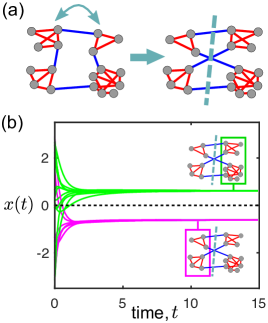
In the synchronization setting, we demonstrate that the presence of sEEPs can induce a bipolar cluster synchronization, in which each group of oscillators may be divided into two ‘out-of-phase’ groups, with trajectories of equal magnitude but opposite sign.
Below, we show how these results appear for signed networks under the MSF framework as well as for Kuramoto oscillators.
Notation:
Our notation is standard. The number of nodes (vertices) in the network is denoted by ; the number of edges (links) by . We denote the adjacency matrix of the graph by , where corresponds to the weight of the coupling between node (oscillator) and . The graph Laplacian matrix is defined as , where is the matrix containing the total coupling strength of each node on the diagonal, i.e., . From this definition, it is straightforward to see that the vector of ones is an eigenvector of with eigenvalue . It is well known that the Laplacian may be decomposed as , where is the node-to-edge incidence matrix and is a diagonal matrix containing the (positive) weights of the edges. It therefore follows that the Laplacian is a positive semidefinite matrix.
To simplify notation, but without loss of generality, our exposition below is presented for unweighted graphs, i.e., . However, all our results apply to weighted graphs by using edge weight matrices appropriately.
II External equitable partitions
External equitable partitions are of interest because the existence of an EEP in a graph has implications for its spectral properties and, consequently, for dynamical processes associated with the graph. EEPs extend the notion of equitable partition (EP). An EP splits the graph into non-overlapping cells (groups of nodes), such that the number of connections to cell from any node is only dependent on . Stated differently, the nodes inside each cell of an EP have the same out-degree pattern with respect to every cell. For EEPs, this requirement is relaxed so that it needs to hold only for the number of connections between different cells ().
Algebraically, these definitions can be represented as follows Cardoso, Delorme, and Rama (2007); Egerstedt et al. (2012); Chan and Godsil (1997). A partition of a graph with nodes into cells is encoded by the indicator matrix : if node is part of cell and otherwise. Hence the columns of are indicator vectors of the cells:
| (1) |
Given the Laplacian matrix of a graph, we can write the definition of an EEP as follows:
| (2) |
Here is the Laplacian of the quotient graph induced by :
| (3) |
where the matrix is the (left) Moore-Penrose pseudoinverse of . Observe that multiplying a vector by from the left sums up the components within each cell, and that is a diagonal matrix with the number of nodes per cell on the diagonal. Hence may be interpreted as a cell averaging operator O’Clery et al. (2013).
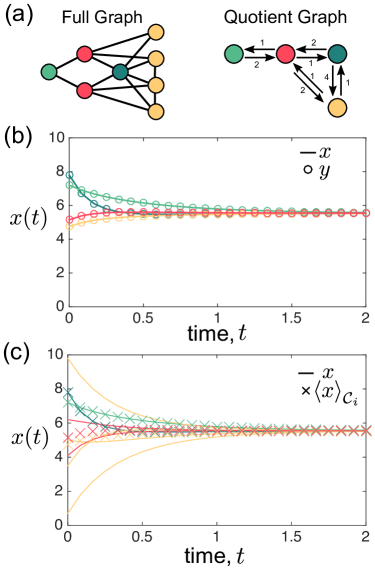
The quotient graph associated with an EEP is a coarse-grained version of the original graph, such that each cell of the partition becomes a new node and the weights between these new nodes are the out-degrees between the cells in the original graph (see Fig. 1a). Although the Laplacian of the original graph is symmetric, the quotient Laplacian will be asymmetric in general. Note that, from the definition of the Laplacian, there is always a trivial EEP in which the whole graph is grouped into one cell, i.e., and .
From (2)–(3), the definition of the EEP can be rewritten solely in terms of :
| (4) |
where is the projection operator onto the cell subspace, i.e., it defines an orthogonal projection onto the range of .
The operator commutes with :
| (5) |
which follows from (2), (4) and the symmetry of and . Using the commutation (5), it is easy to show that:
| (6) |
which summarises the relationship between the cell averaging operator and the Laplacians of
the original and quotient graphs.
Remark 1 [Equitable partitions and coupling via adjacency matrices]: It is instructive to consider EEPs with respect to the stricter requirement of equitable partitions (EPs). Given the adjacency matrix of a graph, an equitable partition encoded by the indicator matrix must fulfil:
| (7) |
Hence we can define the adjacency matrix of the EP quotient graph induced by as:
| (8) |
The adjacency matrix has diagonal entries corresponding to self-loops in the quotient graph of the EP, reflecting the number of edges between any two nodes inside each cell.
In contrast, the adjacency matrix of an EEP cannot be uniquely defined; thus, such in-cell information is not consistently specified.
On the other hand, the quotient graphs of both EPs and EEPs have consistently defined Laplacian matrices, due to the well-known invariance of the Laplacian to the addition of self-loops in a graph,
so that the quotient Laplacian is unaffected by the internal connectivity inside each cell.
This algebraic argument clarifies why EEPs are defined in terms of the Laplacian (2).
It also follows directly that every EP is necessarily an EEP, while the converse is not true.
Remark 2 [Network symmetries and (external) equitable partitions]: Recently, Pecora et al. Pecora et al. (2014); Sorrentino et al. (2016) used the symmetry groups of a graph and their associated irreducible representations to identify possible synchronization clusters in networks of oscillators and to assess their stability. Their group-theoretical analysis is intimately related to the graph-theoretical perspective presented here. Indeed, the symmetry groups of the graph induce orbit partitions. Every orbit partition is an equitable partition, yet the converse is not true: there exist EPs not induced by any symmetry group Kudose (2009); Chan and Godsil (1997). Recall that EEPs are a relaxation of EPs in the sense that EEPs disregard the connections inside each cell. Consequently, EEPs are defined in terms of the Laplacian matrix (2), in contrast to EPs being defined in terms of the adjacency matrix (7). Interestingly, recent work of Sorrentino et al. (2016) introduced ‘adjusted orbit partitions’ induced by symmetry groups of a “dynamically equivalent coupling matrix” in which internal connections inside each cluster are ignored. Such ‘adjusted orbit partitions’ are in fact EEPs but, as for EPs, there exist EEPs that cannot be generated by the symmetry groups of such dynamically equivalent coupling matrices. In this sense, EEPs provide a generalised setting that includes the group-theoretical orbit partitions as a particular case.
As EEPs are a larger class of partitions than EPs and Laplacians are of wide interest in applications, we concentrate here on networks with Laplacian coupling. All our results can be applied straightforwardly to systems in which the coupling is described by the adjacency matrix, by considering EPs rather than EEPs.
III Cluster synchronization under the external equitable partition
We first use EEPs to study cluster synchronization on standard networks, i.e., defined by connected undirected graphs with positive weights. We start by considering results for linear consensus, and then apply the framework to nonlinear cluster synchronization both under the MSF formalism as well as Kuramoto networks.
III.1 Dynamical implications of EEPs: the linear case
The definition of the EEP (2) can be understood as a ‘quasi-commutation’ relation, which signals a certain invariance of the partition encoded by with respect to the Laplacian . Similarly, Eq. (6) shows that the cell averaging operator exhibits a (distinct) invariance with respect to . In particular, Eq. (2) implies that the associated cell indicator matrix spans an invariant subspace of , whence it follows that there exists a set of eigenvectors which is localised on the cells of the partition. Furthermore, the eigenvalues associated with the eigenvectors spanning the invariant subspace are shared with , the Laplacian of the quotient graph O’Clery et al. (2013). If has degenerate eigenvalues, an eigenbasis can still be chosen so that it is localised on the cells of the partition O’Clery et al. (2013).
The properties of the EEP (2)–(6) have noteworthy consequences for linear dynamics dictated by , as illustrated by the case of linear consensus dynamics O’Clery et al. (2013):
| (9) |
where the vector describes the state of the system.
First, as shown in Fig. 1b, the EEP is consistent with a form of invariance akin to ‘cluster consensus’. In particular, if the initial state vector is given by for some arbitrary (i.e., all the nodes within cell have the same value ), the nodes inside the cells remain identical for all times and their dynamics is governed by the quotient graph:
| (10) |
This follows directly from .
Second, the dynamics of the cell-averaged states is governed by the quotient graph:
| (11) |
which follows from . Thus, the cell-averaged dynamics is governed by a lower dimensional linear model, with dimensionality equal to the number of cells in the EEP (see Fig. 1c).
Third, the results obtained for the autonomous dynamics with no inputs (9) can be equivalently rephrased for the system with a bounded input :
| (12) |
In particular, similarly to (10), we also have cell invariance under inputs: if we apply an input consistent with the cells of an EEP (i.e., ), the nodes inside each cell remain identical for all times O’Clery et al. (2013). This simple insight, which follows from the impulse-response of the linear system (12), will be useful when analysing nonlinear synchronization protocols.
Finally, it is important to remark that since there is always a trivial EEP spanning the complete graph (with ), all the results above and henceforth can be trivially applied to the case of global consensus (global synchronization) as a particular case.
III.2 EEPs and nonlinear cluster synchronization within the MSF framework
We now extend the notions introduced above to a more general setting describing the dynamics of interconnected nonlinear systems. This framework is known as the Master Stability Function (MSF) and has been pioneered by Pecora and co-workers Heagy, Carroll, and Pecora (1994); Pecora and Carroll (1998); Barahona and Pecora (2002).
We consider networks of identical coupled oscillatory nonlinear systems in which the dynamics of each node is described by:
| (13) |
where is a parameter that regulates the coupling strength; is the state vector of node ; is the intrinsic dynamics of each node; and the coupling function specifies how the nodes in the network interact according to the interconnection topology described by the graph Laplacian .
Although, as discussed above, we could consider a coupling mediated by the adjacency matrix (and associated EPs), we concentrate here on the case of Laplacian coupling (and associated EEPs) as the more generic case of interest in the literature .
To facilitate the subsequent discussion, we define and use the Kronecker product to rewrite (13) compactly as a -dimensional system of ODEs:
| (14) |
where , and is the -dimensional identity matrix.
A cluster-synchronized state consistent with an EEP with indicator matrix is then given by:
| (15) | ||||
| (16) |
III.2.1 EEPs and invariance of cluster-synchronized states
Let a graph with Laplacian exhibit a non trivial EEP with cells encoded by the indicator matrix and quotient Laplacian . The dynamics of the cell variables associated with the quotient graph is then given by
| (17) |
where are defined analogously to above, and we have the relations:
| (18) | ||||
| (19) |
In close parallel to the linear case (10), we can derive the following result for cluster-synchronized dynamics. Let us have an initial condition that is identical within the cells of the EEP, i.e., for some arbitrary at . Then the nodes within cells of the EEP remain identical for all time , and their dynamics can be described by the dynamics of the quotient graph:
| (20) | ||||
This result follows from:
Here we have made use of the standard identity .
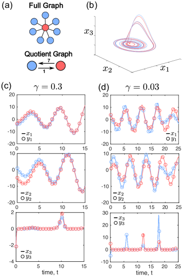
Example [Coupled Rössler oscillators]: Consider a network of oscillators where each node has a three dimensional dynamics () given by the chaotic Rössler system Rössler (1976)
| (21) |
with parameters and . The oscillators are coupled through the variable according to the linear function:
The topology of interconnection is a star graph, which has an EEP with two cells (): one cell comprises the central node, the other cell contains all other nodes (Fig. 2).
Let the initial condition be . Then the variables of the nodes within each cell remain identical at all times, i.e., the dynamics stays cluster-synchronized (Fig. 2). For , this poly-synchronous state (while remaining cluster-synchronized at all times) evolves towards the globally synchronized state (Fig. 2c). In contrast, for , the cluster synchronization of the cells does not converge towards global synchrony, since the completely synchronized state of the quotient graph dynamics is no longer (linearly) stable (Fig. 2d and Sec. III.2.3).
III.2.2 EEPs and cell-averaged synchronization dynamics
Although the invariance of cluster-synchronized EEP states carries over to the nonlinear MSF setting, the second finding of the linear analysis, namely that the dynamics of cell averages is described by the quotient graph dynamics (17), does not hold in general. Indeed, after some algebraic manipulations it is easy to see that:
Due to their nonlinearity, in general and do not commute with the linear cell-averaging operation:
Hence, unlike the linear case, the cell-averaged dynamics is not strictly equivalent to the synchronization dynamics governed by the Laplacian of the quotient graph.
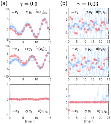
However, an approximate equivalence is obtained if we consider an perturbation around a cluster-synchronized state (15). To first order we then have,
where and denote the Jacobians of and for state .
This result implies that if the cluster-synchronized state is stable, the averaging operator will approximately commute with both and when the state is close to the cluster-synchronized state. As a consequence, an appropriately chosen initial condition of the average cell dynamics will remain close (or converge) to the quotient dynamics, as seen in Fig. 3a. On the other hand, the interplay of the Jacobians of and and the graph structure encoded by and can render the initial perturbation unstable, and the state will exponentially diverge. In that case, the quotient dynamics will not be a good model for the cell-averaged dynamics, as seen in Fig. 3b. We explore these points through the MSF formalism in Section III.2.3, where we consider the stability of the cluster-synchronized state (including the globally synchronized state).
III.2.3 Stability of EEP cluster-synchronized states through the MSF formalism
The sections above lead naturally to consider the stability of EEP cluster synchronization. Following Pecora et al Pecora et al. (2014); Sorrentino et al. (2016), the linearized stability around any cluster synchronized state can be evaluated using the MSF framework via the variational expression:
| (22) |
where is the (consistent) state of every node in the th cluster, as defined in (15), and are identity matrices consigned to each cluster:
| (23) |
as given by the cell indicator vectors (1). Using computational group theory, Pecora et al. block-diagonalize the above expression to assess the stability of any cluster-synchronized state.
As an alternative to symmetry-based arguments, the MSF variational analysis may also be understood using EEPs and their associated indicator matrices. Here we use the fact that eigenvectors and eigenvalues are shared between the Laplacians of the original and quotient graphs O’Clery et al. (2013). Let us denote the eigenvectors of the quotient Laplacian by with eigenvalues such that . The properties of the EEP O’Clery et al. (2013) ensure that a subset of the eigenvectors of the full Laplacian are directly related to the eigenvectors of :
| (24) |
These are the eigenvectors that define the cluster synchronization manifold commensurate with the EEP. The eigenvectors orthogonal (transversal) to the cluster-synchronized manifold are denoted by . These are the eigenmodes that drive the system out of a cluster-synchronized state, and therefore we want these modes to be damped. An orthogonal matrix of eigenvectors of that diagonalizes the Laplacian:
| (25) |
is thus given by
| (26) |
Hence the first columns correspond to eigenvectors of (with eigenvalues ) that can be mapped to , and the second block of columns corresponds to the transversal manifold.
Using to diagonalize via the coordinate transformation leads to:
| (27) | ||||
| (28) | ||||
| (29) |
where we have
| (30) |
The structure of the matrices means that the modes in the cluster synchronization manifold are effectively decoupled from the modes transversal to it. To see this, note that from and (24) it follows that the transversal eigenvectors lie in the orthogonal subspace to : . (This also means that every transversal mode is mean-free within each cell: .) Therefore, we have the following effective decoupling between the cluster-synchronized and transversal modes:
leading to
By examining this matrix, we can obtain information about the (local) stability of the cluster-synchronized state (see Ref. Sorrentino et al. (2016) for a related discussion). In order to check the linear stability of the cluster-synchronized manifold, it is enough to check that all the transversal modes are damped. Yet such damping of the transversal modes alone does not specify the behavior within the cluster-synchronized manifold, or indeed the convergence towards any of the different cluster-synchronized states within it. Further damping within the cluster-synchronized manifold would lead the dynamics to converge to an even lower-dimensional manifold, i.e., towards a particular subset of the cluster-synchronized states. Stated differently, some of the cells in a cluster-synchronized state could merge, leading to another state with fewer cells. If damping within the manifold is present, it can lead to convergence towards the completely synchronized state, akin to the numerics in Fig. 2c (and in contrast to the numerics in Fig. 2d where such convergence within the manifold is not observed).
III.3 EEP cluster synchronization in Kuramoto networks
The MSF framework provides a powerful tool for the analysis of nonlinear systems with diffusive couplings, yet there are important classes of systems that do not lend themselves naturally to this formulation. Examples include systems with sinusoidal coupling between oscillators, as in models of power systems Dörfler and Bullo (2012) or the classic Kuramoto model of coupled oscillators Kuramoto (1975, 2012). The use of EEPs can nevertheless afford us insight into cluster synchronization in these cases, too.
We consider the Kuramoto model with oscillators
| (31) |
where and describe the phase and intrinsic frequency of each oscillator, respectively, is the coupling parameter, and is the adjacency matrix encoding the network connectivity.
To simplify our notation below, let us renormalize time . The dynamics of a network of Kuramoto oscillators coupled through a graph with Laplacian , where is the incidence matrix of the graph, can then be rewritten in vector-matrix notation as Jadbabaie, Motee, and Barahona (2004):
| (32) | ||||
| (33) |
where and are -dimensional vectors, and we have defined
This rewriting emphasizes the close relation of the Kuramoto model to Laplacian dynamics. Not only does the linearization for small phase differences lead to the standard linear Laplacian dynamics, but the final equality underscores the fact that the full Kuramoto model may still be understood in terms of a weighted Laplacian dynamics with time-varying edge weights Jadbabaie, Motee, and Barahona (2004):
| (34) |
It is therefore not surprising that EEPs give useful insights into invariant dynamics of Kuramoto networks.
III.3.1 Case I: equal intrinsic frequencies
Let us consider first the case where all intrinsic frequencies are identical: . In this case, we may assume without loss of generality, as this is equivalent to grounding the system or defining the phases with reference to a rotating frame Jadbabaie, Motee, and Barahona (2004). The resulting system
| (35) |
is well known to converge Jadbabaie, Motee, and Barahona (2004); Dörfler and Bullo (2014) to the totally synchronized state with identical phases.
Let the graph with Laplacian be endowed with an EEP with partition matrix . We can then define the following Kuramoto dynamics taking place on the quotient graph of the EEP:
| (36) |
where is the -dimensional vector containing the phases associated with the quotient graph, and we use the definition (3) to factorize the quotient Laplacian appropriately:
| (37) |
As for the linear case (10), we wish to show that the cell dynamics on the quotient graph (36) describes an invariant dynamics of cluster-synchronized states in the full model (35). In other words, we need to show that
| (38) |
i.e., is invariant under the full dynamics.
To establish this, we use the following fact:
A given EEP for a network remains an EEP if all edge weights between two distinct cells are multiplied by a factor that depends only on the two cells.
This fact is a direct consequence of the definition of an EEP, since such scaling changes the
out-degree patterns of all nodes within a cell consistently.
Remark 3 [EEPs and structured weights]: A particular case of such a rescaling that will be useful below can be represented algebraically as follows. Consider a graph with Laplacian and an EEP with indicator matrix . Let the edge weights be scaled consistently across cells (in the above sense) leading to the modified Laplacian:
| (39) |
where is a cell vector, and is a symmetric function applied element-wise. Since the EEP remains unchanged under this rescaling, it follows from (5) that the projection operator associated with also commutes with the modified Laplacian:
| (40) |
We now use (40) to show that EEP cluster-synchronized states are invariant under Kuramoto dynamics. To see this, left multiply (36) with :
where follows from the definition of the projection operator. Note that is symmetric.
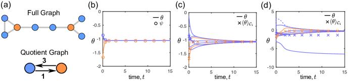
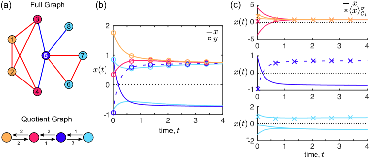
The proof shows that the full Kuramoto model follows the quotient dynamics (36) for all times, if it ever synchronizes to a particular EEP. We illustrate this behavior in Fig. 4b, where we use a network topology (Fig. 4a) inspired by a construction outlined by Chan and Godsil Chan and Godsil (1997); Kudose (2009) highlighting the difference between orbit partitions (generated from symmetry groups) and equitable partitions.
As shown in Fig. 4c, the cell averages are also well described by the quotient dynamics provided the initial condition is not too far away from the EEP-averaged state. If the phases of the initial condition are outside the open semicircle (as in Fig. 4d), a naive linear averaging does not fully capture the convergence on the torus.

III.3.2 Case II: non-equal intrinsic frequencies commensurate with an EEP
The analysis for the Kuramoto model with equal frequencies does not apply in general to a network of oscillators with non-equal intrinsic frequencies. However, similar results hold when the oscillators within each cell have the same frequency. In particular, consider the Kuramoto system (32) with EEP-commensurate frequencies:
| (41) |
where is a -dimensional vector containing the frequencies of the cells.
In the case of heterogeneous frequencies, the model can not reach globally identical synchronization, so the ‘most synchronous’ behavior is the cluster-synchronized state with identical phases within each cell. By the arguments in Section III.3.1, mutatis mutandis, it is easy to see that the cluster-synchronized state is invariant under (41) and governed by the quotient graph:
| (42) |
A numerical illustration of this invariance is given in Figure 5. We note that there is a close analogy here to the scenario of the linear consensus system with an input commensurate with the EEP (12). Indeed, the intrinsic frequencies of the cells can be interpreted as constant inputs to each of the cells.
We remark that our results for Kuramoto systems here are concerned with the invariance of solutions
and not their stability. As studied previously Jadbabaie, Motee, and Barahona (2004); Dörfler and Bullo (2014),
the stability of the synchronous state depends on the magnitude of the spread of the
frequencies along the edges of the graph relative to the coupling parameter .
Hence as the coupling becomes smaller, and the norm of becomes larger, the synchronized (and cluster-synchronized) solutions become unstable.
Remark 4 [Kuramoto model with a phase offset]: To gain insight into the effect of a phase offset, let us consider the Kuramoto model with equal intrinsic frequencies and a constant phase offset discussed in Ref. Nicosia et al. (2013), which can be rewritten as:
| (43) | ||||
| (44) |
For , the first term vanishes, and we recover the standard Kuramoto model for which the EEP analysis holds. Therefore, if is within (close proximity to) the cluster synchronization manifold , by our arguments above, the system will remain in a polysynchronous, clustered state. As increases, the magnitude of the Kuramoto coupling parameter ( decreases, whereas at the same time the magnitude of the spread of the input intrinsic frequencies ( increases. Hence, as is increased above a threshold, we expect the cluster synchronization manifold to lose stability, as for the case of non-equal frequencies above. This is in line with Nicosia et al. (2013), who observed numerically that cluster synchrony is lost above a critical value of .
IV Cluster synchronization in networks with positive and negative weights
Many mathematical models for real-world networks need to incorporate positive and negative interactions. For instance, in social networks, relationships can be friendly or hostile, or they reflect trust or distrust between individuals. Therefore, the sign of a link is a central concept in social psychology, associated with the emergence of conflict and tension in social systems Heider (1946); Cartwright and Harary (1956), and it has gained popularity recently in the study of online social networks Leskovec, Huttenlocher, and Kleinberg (2010) and online cooperation Szell, Lambiotte, and Thurner (2010). In biological systems, the sign of an edge is also a key element, in particular when modelling dynamical processes. For instance, genes can either promote or repress the expression of other genes in genetic regulatory networks Davidson and Levin (2005), and neurons can excite or inhibit the firing of other neurons in neuronal networks and thereby shape the global dynamics of the system Gerstner et al. (2014); Schaub et al. (2015).
IV.1 Signed networks and structural balance: the signed external equitable partition
IV.1.1 The signed Laplacian matrix
For a network with positive and negative interactions, we can define the signed Laplacian matrix of the network as follows Altafini (2013a); Kunegis et al. (2010):
| (45) |
where is the diagonal absolute degree matrix, and is again the adjacency matrix (which may hereafter contain both positive and negative weights). As for the standard Laplacian, it can be shown that the signed Laplacian is positive semidefinite and its spectrum contains one zero eigenvalue when the graph is connected and structurally balanced. To see this, note that the signed Laplacian can be expressed as:
| (46) |
where is the absolute edge weight matrix and is the signed node-to-edge incidence matrix:
Henceforth, we assume without loss of generality. By using the signed Laplacian, the construction of an EEP can be extended to signed graphs. To do so, however, we must first introduce the notion of structurally balanced graph, which will enable us to define the notion of a signed external equitable partition (sEEP).
IV.1.2 Structurally balanced graphs
Following Cartwright and Harary Cartwright and Harary (1956), a signed graph is defined to be structurally balanced if the product of the signs along any closed path in the network is positive. This definition implies that only ‘consistent’ social relationships are allowed in triangles of three nodes: either all interactions are positive, or there are exactly 2 negative links, which may be interpreted in the sense that “the enemy of my enemy is my friend” Heider (1946). Equivalently, a signed network is structurally balanced if it can be split into two factions, where each faction contains only positive interactions internally, while the connections between the two factions are purely antagonistic (see Fig. 6). It has been shown that many social networks are close to being structurally balanced Facchetti, Iacono, and Altafini (2011), suggesting that there might be a dynamical process acting on such systems driving them towards structural balance Marvel et al. (2011); Traag, Van Dooren, and De Leenheer (2013).
The following characterization of a structurally balanced graph based on the signed Laplacian was highlighted by Altafini Altafini (2013a, b). A network is structurally balanced if there exists a diagonal matrix , with on the diagonal, such that the matrix:
| (47) |
contains only negative elements on the off-diagonal. In other words, the signed Laplacian can be transformed into the standard Laplacian of an associated graph with only positive weights through the similarity transformation defined by . The matrix is called switching equivalence, signature similarity, or gauge transformation in the literature Altafini (2013b). Using this characterization, one can efficiently determine whether a network is structurally balanced Facchetti, Iacono, and Altafini (2011) and obtain the corresponding switching equivalence matrix . Note that it follows trivially that a standard network with only positive weights is always structurally balanced with . Hence is a generalization of the standard Laplacian.
IV.1.3 Signed external equitable partitions
Using the signed Laplacian, we extend the concept of EEP to structurally balanced signed networks. Consider a structurally balanced signed graph with signed Laplacian and denote the Laplacian of the positive switching equivalent graph by . Let denote the indicator matrix of an EEP of :
| (48) |
Then there exists a signed indicator matrix that defines an invariant subspace for :
| (49) |
which follows from the definition (47) and .
We define the partition with indicator matrix as the signed external equitable partition (sEEP), and its associated quotient graph is given by:
| (50) |
Therefore cells in a sEEP contain nodes with the same out-degree pattern in absolute value. An illustration of a sEEP and associated quotient graph is shown in Fig. 7. Note that the quotient graph only has positive weights.
IV.2 Dynamics and signed external equitable partitions
The definition of a sEEP provides us with an appropriate tool for the analysis of cluster synchronization in structurally balanced signed networks, as we now show. The results in this section parallel those obtained for unsigned graphs, hence we concentrate on the distinctive features of clustered dynamics in signed networks.
IV.2.1 The linear case: bipolar cluster synchronization in signed consensus dynamics
A remarkable feature of structurally balanced networks is that the linear signed consensus dynamics Altafini (2013a):
| (51) |
converges to a polarized state, in which the nodes are divided into two sets with final values that are equal in magnitude but opposite in sign (Fig. 6). Stated differently, the eigenvector of associated with the zero eigenvalue has the form , where . As shown in Ref. Altafini (2013a), this implies that the system dynamics (51) converges to the final state
| (52) |
and the sign pattern of the eigenvector corresponds precisely to the switching equivalence transformation, i.e., . In the following, we will refer to as the polarization of node . Note that the the vector is only defined up to an arbitrary sign, so only the relative polarization of the nodes is relevant.
We now extend the analysis to networks endowed with a sEEP. The presence of a sEEP (49) has similar dynamical implications to the presence of an EEP in the case of a positive graph. The following statements can be proved analogously to the standard (unsigned) consensus case.
First, sEEP cluster-synchronized states are invariant under the full linear dynamics (51). Hence, given an initial condition consistent with a sEEP, remains in the sEEP state for all times, and the dynamics is governed by the quotient graph: (see Figure 7b).
In contrast to standard unsigned graphs, the variable of every node within a cell of the cluster-synchronized state will have the same magnitude, but its sign may be inverted depending on its polarization . Therefore, in signed networks each cell maybe itself divided into two factions whose values are of equal magnitude (as given by the quotient dynamics), but of opposite sign, as illustrated in Figure 7 (see how node has the opposite sign to nodes all in the cyan cell). We use the term bipolar cluster synchronization to account for this phenomenon in signed networks.
Second, the signed cell-averaged dynamics is determined by the dynamics of the quotient graph (Fig. 7c). The signed consensus dynamics approaches the bipolar consensus (52), and the final sign of each node variable is determined by , as seen in Fig. 7c for nodes and (positively polarized) and nodes (negatively polarized).
Third, a system with inputs aligned with the sEEP
| (53) |
exhibits a bipolar cluster-synchronized state. To see this, consider the component of the state orthogonal to the bipolar cluster synchronization manifold:
| (54) |
which has a dynamics , and the orthogonal component decays asymptotically to
| (55) |
since Hence the system converges to the sEEP manifold.
IV.2.2 Bipolar cluster synchronization for nonlinear dynamics with Laplacian couplings
All the results obtained in Section III.2 apply to nonlinear dynamics on signed networks of the form:
| (56) |
but now with the additional feature that the dynamics can support a bipolar cluster synchronization based on a sEEP. We do not discuss this case in detail again, instead we illustrate these findings for signed Kuramoto networks.
IV.2.3 Bipolar cluster synchronization in signed Kuramoto networks
While standard Kuramoto networks with positive couplings have been studied extensively Rodrigues et al. (2016), the literature on Kuramoto networks with both attractive (positive) and repulsive (negative) couplings is comparatively sparse, with only a handful of mean-field results El-Ati and Panteley (2013).
Using the definition of the signed Laplacian, we write the Kuramoto model on a signed graph as:
| (57) |
Likewise, the Kuramoto dynamics on the quotient graph becomes:
| (58) |
For structurally balanced signed networks, making the necessary adjustments for the switching equivalence , we then reach the same conclusions as in Section III.3.
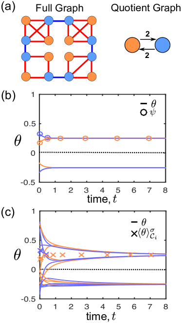
In Figure 8, we provide numerical examples that replicate our findings for signed graphs. As expected, in Figure 8b) we see that a bipolar cluster-synchronized solution remains invariant for all times. Figure 8c) shows that for an initial condition that is not too spread out on the unit circle, we observe numerically that the (sign adjusted) cell-averaged is well aligned with the quotient dynamics. For non-identical intrinsic frequencies commensurate with the sEEP, the Kuramoto model converges to a final state consistent with the cells of the sEEP, yet exhibiting out-of-phase behavior within each cell due to the polarization of the nodes.
V Discussion
In this paper, we have shown how to coarse-grain the dynamics of generic synchronization processes by using the graph-theoretical framework of external equitable partitions. Exploiting regularities present in the underlying coupling network, EEPs give clusters of nodes that play an equivalent dynamical role O’Clery et al. (2013). The resulting coarse-grained dynamics corresponds to cluster synchronization, in which all nodes within a cell follow the same trajectory. Importantly, one can extend the notion of EEPs to other types of coupling schemes, as shown by our analysis of signed networks. In structurally balanced signed networks, we showed that each of the cells splits into two ‘out-of-phase’ dynamical factions, with the same magnitude but opposite sign.
Connections with symmetry groups.
We have shown how our graph-theoretical approach complements the use of symmetry groups for the analysis of synchronization dynamics over networks Pecora et al. (2014); Sorrentino et al. (2016); Barahona et al. (1997). As discussed in Pecora et al. (2014), there exist efficient software tools to compute symmetry groups in networks Darga, Sakallah, and Markov (2008); Group and hence orbit partitions Pecora et al. (2014); Sorrentino et al. (2016). The more general problem of obtaining all EEPs for a graph appears to be computationally more challenging Kamei and Cock (2013); Sorrentino et al. (2016). However, there exist efficient algorithms to compute EEPs centered around a node O’Clery et al. (2013); Cao, Zhang, and Camlibel (2013), which can be used to characterize the dynamical influence of particular nodes on the global dynamics of the network Martini, Egerstedt, and Bicchi (2010); Egerstedt et al. (2012); O’Clery et al. (2013).
Other signed coupling schemes.
We have chosen to consider couplings given by the signed Laplacian , as it provides a direct generalization of the standard Laplacian and has direct connections with dynamical properties. In particular, the positive semi-definiteness of allows us to express the Kuramoto model in terms of signed incidence matrices (57), thus facilitating our proof and interpretation. However, the ideas developed here may be applied to other signed coupling schemes, provided the equivalent invariance condition to (2) can be found. For instance, another interesting coupling is given by the Laplacian , where is a signed adjacency matrix and . For the network in Fig. 7a, the EEP with respect to Laplacian is almost identical to the one with respect to , except that node forms its own cell. It is worth remarking, however, that while the algebraic characterization of such invariant partitions can still be exploited, the graph-theoretical notion of ’equitability’, related to the combinatorial count of inter-cell degrees, can be lost. As many algorithms leverage such combinatorial properties to search for EEPs, this may make the presence of such invariant partitions harder to detect. Furthermore, their dynamical interpretation might be problematic in generic systems since (and other coupling matrices) will in general be indefinite, hence impacting the dynamical stability.
Relation to other synchronization notions.
Because EEPs exploit the graph structure in connection with dynamics, our approach complements other methods for the analysis of synchronization. Here, we have concentrated on the existence and invariance of cluster-synchronized states, with some discussion of their stability in the context of the MSF. Further insights could be gained by combining our EEP-based analysis with other methodologies, such as the analysis of potential energy coupling landscapes or various mean-field analyses (see Refs.Dörfler and Bullo (2014); Arenas et al. (2008); Rodrigues et al. (2016) for overviews). In particular, as EEPs are linked to the existence of invariant subspaces, contraction-based arguments may be fruitfully applied to global system dynamics in such networks Moreau (2004); Sepulchre (2011); Russo and Slotine (2011); Mauroy and Sepulchre (2012).
A particular notion of synchronization worth mentioning is that of chimera states Panaggio and Abrams (2015); Abrams and Strogatz (2004), in which parts of the network act in unison while another parts appear unsynchronized. One may conjecture that a possible mechanism to reach such a state is to endow the underlying network with an EEP comprising one large cell and a multitude of single node cells. If, by carefully configuring the dynamics, the large cell could be made to remain stable while the single node cells follow independent trajectories, a chimera state might be obtained.
Future work.
Several other avenues of future work appear to be worth pursuing. As the idea of signed networks and social balance is at the core of social network theory Doreian and Mrvar (1996); Cartwright and Harary (1956); Heider (1946), it would be important to investigate if the bipolar cluster synchronization described here can be related to models evolving towards structural balance Marvel et al. (2011); Traag, Van Dooren, and De Leenheer (2013). Following the insight by Hendrickx Hendrickx (2014) that signed opinion dynamics can be understood as a dimensional dynamics with positive interactions, it would also be interesting to understand the symmetry requirements that an EEP implies on the lifted -dimensional graph, and whether the EEP could be used to elucidate further properties.
Another extension would be to relax the strict requirements of EEPs (e.g., by allowing minor perturbations on a graph with an EEP) in order to study how the dynamics of the system is affected. Generalizations of EEPs that allow different kinds of couplings (e.g., directed, time-varying Scardovi and Sepulchre (2009); Paley et al. (2007), delays Papachristodoulou, Jadbabaie, and Munz (2010)) would also be of interest.
Finally, it is worth remarking that while we focussed here on the dynamics of synchronization in linear (consensus) and nonlinear processes (coupled oscillators, Kuramoto), the concept of external equitable partitions is applicable to more general scenarios where agents interact over a graph structure. The key ingredient is the presence of a low-dimensional invariant subspace in the coupling (spanned by the partition matrix) which can be exploited to obtain a dynamical dimensionality reduction leading to a coarse-grained system description. While EEPs have been used in consensus and control, other application areas such as ecological networks or chemical reaction networks would be worth investigating.
Acknowledgments
We thank Karol Bacik for comments and carefully reading the manuscript. MTS, JCD, RL acknowledge support from: FRS-FNRS; the Belgian Network DYSCO (Dynamical Systems, Control and Optimisation) funded by the Interuniversity Attraction Poles Programme initiated by the Belgian State Science Policy Office; and the ARC (Action de Recherche Concerte) on Mining and Optimization of Big Data Models funded by the Wallonia-Brussels Federation. NO’C was funded by a Wellcome Trust Doctoral Studentship at Imperial College London during this work. YNB thanks the G. Harold & Leila Y. Mathers Foundation. MB acknowledges support through EPSRC grants EP/I017267/1 and EP/N014529/1.
No new data was collected in the course of this research.
References
- Strogatz (2000) S. H. Strogatz, “From Kuramoto to Crawford: exploring the onset of synchronization in populations of coupled oscillators,” Physica D: Nonlinear Phenomena 143, 1–20 (2000).
- Boccaletti et al. (2002) S. Boccaletti, J. Kurths, G. Osipov, D. Valladares, and C. Zhou, “The synchronization of chaotic systems,” Physics Reports 366, 1–101 (2002).
- Arenas et al. (2008) A. Arenas, A. Díaz-Guilera, J. Kurths, Y. Moreno, and C. Zhou, “Synchronization in complex networks,” Physics Reports 469, 93–153 (2008).
- Dörfler and Bullo (2014) F. Dörfler and F. Bullo, “Synchronization in complex networks of phase oscillators: A survey,” Automatica 50, 1539–1564 (2014).
- Nishikawa and Motter (2015) T. Nishikawa and A. E. Motter, “Comparative analysis of existing models for power-grid synchronization,” New Journal of Physics 17, 015012– (2015).
- Panaggio and Abrams (2015) M. J. Panaggio and D. M. Abrams, “Chimera states: coexistence of coherence and incoherence in networks of coupled oscillators,” Nonlinearity 28, R67– (2015).
- Rodrigues et al. (2016) F. A. Rodrigues, T. K. D. Peron, P. Ji, and J. Kurths, “The Kuramoto model in complex networks,” Physics Reports 610, 1–98 (2016).
- Kuramoto (2012) Y. Kuramoto, Chemical oscillations, waves, and turbulence, Vol. 19 (Springer Science & Business Media, 2012).
- Jadbabaie, Lin, and Morse (2003) A. Jadbabaie, J. Lin, and A. S. Morse, “Coordination of groups of mobile autonomous agents using nearest neighbor rules,” IEEE Transactions on Automatic Control 48, 988–1001 (2003).
- Heagy, Carroll, and Pecora (1994) J. Heagy, T. Carroll, and L. Pecora, “Synchronous chaos in coupled oscillator systems,” Physical Review E 50, 1874 (1994).
- Pecora and Carroll (1998) L. M. Pecora and T. L. Carroll, “Master stability functions for synchronized coupled systems,” Physical Review Letters 80, 2109 (1998).
- Barahona and Pecora (2002) M. Barahona and L. M. Pecora, “Synchronization in Small-World Systems,” Phys. Rev. Lett. 89, 054101 (2002).
- Pecora and Barahona (2005) L. M. Pecora and M. Barahona, “Synchronization of oscillators in complex networks,” Chaos and Complexity Letters 1, 61–91 (2005).
- Jadbabaie, Motee, and Barahona (2004) A. Jadbabaie, N. Motee, and M. Barahona, “On the stability of the Kuramoto model of coupled nonlinear oscillators,” in Proceedings of the American Control Conference, 2004., Vol. 5 (2004) pp. 4296 –4301.
- Judd (2013) K. Judd, “Networked dynamical systems with linear coupling: synchronisation patterns, coherence and other behaviours,” Chaos: An Interdisciplinary Journal of Nonlinear Science 23, 043112 (2013).
- D’Huys et al. (2008) O. D’Huys, R. Vicente, T. Erneux, J. Danckaert, and I. Fischer, “Synchronization properties of network motifs: Influence of coupling delay and symmetry,” Chaos 18, 037116 (2008).
- Lu, Liu, and Chen (2010) W. Lu, B. Liu, and T. Chen, “Cluster synchronization in networks of coupled nonidentical dynamical systems,” Chaos: An Interdisciplinary Journal of Nonlinear Science 20, 013120 (2010).
- Dahms, Lehnert, and Schöll (2012) T. Dahms, J. Lehnert, and E. Schöll, “Cluster and group synchronization in delay-coupled networks,” Physical Review E 86, 016202 (2012).
- Do, Höfener, and Gross (2012) A.-L. Do, J. Höfener, and T. Gross, “Engineering mesoscale structures with distinct dynamical implications,” New Journal of Physics 14, 115022– (2012).
- Fu et al. (2013) C. Fu, Z. Deng, L. Huang, and X. Wang, “Topological control of synchronous patterns in systems of networked chaotic oscillators,” Phys. Rev. E 87, 032909– (2013).
- Rosin et al. (2013) D. P. Rosin, D. Rontani, D. J. Gauthier, and E. Schöll, “Control of Synchronization Patterns in Neural-like Boolean Networks,” Phys. Rev. Lett. 110, 104102– (2013).
- Sorrentino and Ott (2007) F. Sorrentino and E. Ott, “Network synchronization of groups,” Phys. Rev. E 76, 056114– (2007).
- Williams et al. (2013) C. R. S. Williams, T. E. Murphy, R. Roy, F. Sorrentino, T. Dahms, and E. Schöll, “Experimental Observations of Group Synchrony in a System of Chaotic Optoelectronic Oscillators,” Phys. Rev. Lett. 110, 064104– (2013).
- Pecora et al. (2014) L. M. Pecora, F. Sorrentino, A. M. Hagerstrom, T. E. Murphy, and R. Roy, “Cluster synchronization and isolated desynchronization in complex networks with symmetries,” Nature communications 5 (2014).
- Sorrentino et al. (2016) F. Sorrentino, L. M. Pecora, A. M. Hagerstrom, T. E. Murphy, and R. Roy, “Complete characterization of the stability of cluster synchronization in complex dynamical networks,” Science Advances 2 (2016), 10.1126/sciadv.1501737.
- Egerstedt et al. (2012) M. Egerstedt, S. Martini, M. Cao, K. Camlibel, and A. Bicchi, “Interacting with Networks: How Does Structure Relate to Controllability in Single-Leader, Consensus Networks?” Control Systems, IEEE 32, 66–73 (2012).
- O’Clery et al. (2013) N. O’Clery, Y. Yuan, G.-B. Stan, and M. Barahona, “Observability and coarse graining of consensus dynamics through the external equitable partition,” Physical Review E 88, 042805 (2013).
- Cardoso, Delorme, and Rama (2007) D. M. Cardoso, C. Delorme, and P. Rama, “Laplacian eigenvectors and eigenvalues and almost equitable partitions,” European Journal of Combinatorics 28, 665–673 (2007).
- Martini, Egerstedt, and Bicchi (2010) S. Martini, M. Egerstedt, and A. Bicchi, “Controllability analysis of multi-agent systems using relaxed equitable partitions,” International Journal of Systems, Control and Communications 2, 100–121 (2010).
- Kuramoto (1975) Y. Kuramoto, “Self-entrainment of a population of coupled non-linear oscillators,” in International Symposium on Mathematical Problems in Theoretical Physics (Springer, 1975) pp. 420–422.
- Heider (1946) F. Heider, “Attitudes and cognitive organization,” The Journal of Psychology 21, 107–112 (1946).
- Cartwright and Harary (1956) D. Cartwright and F. Harary, “Structural balance: a generalization of Heider’s theory.” Psychological Review 63, 277 (1956).
- Altafini (2013a) C. Altafini, “Consensus Problems on Networks With Antagonistic Interactions,” Automatic Control, IEEE Transactions on 58, 935–946 (2013a).
- Altafini (2013b) C. Altafini, “Stability analysis of diagonally equipotent matrices,” Automatica 49, 2780 – 2785 (2013b).
- Chan and Godsil (1997) A. Chan and C. D. Godsil, “Symmetry and eigenvectors,” in Graph Symmetry (Springer, 1997) pp. 75–106.
- Kudose (2009) S. Kudose, “Equitable Partitions and Orbit Partitions,” http://www.math.uchicago.edu/~may/VIGRE/VIGRE2009/REUPapers/Kudose.pdf (2009).
- Rössler (1976) O. E. Rössler, “An equation for continuous chaos,” Physics Letters A 57, 397–398 (1976).
- Dörfler and Bullo (2012) F. Dörfler and F. Bullo, “Synchronization and transient Stability in Power Networks and nonuniform Kuramoto oscillators,” SIAM Journal of Control and Optimization 50, 1616–1642 (2012).
- Nicosia et al. (2013) V. Nicosia, M. Valencia, M. Chavez, A. Díaz-Guilera, and V. Latora, “Remote synchronization reveals network symmetries and functional modules,” Physical Review Letters 110, 174102 (2013).
- Leskovec, Huttenlocher, and Kleinberg (2010) J. Leskovec, D. Huttenlocher, and J. Kleinberg, “Signed networks in social media,” in Proceedings of the SIGCHI conference on human factors in computing systems (ACM, 2010) pp. 1361–1370.
- Szell, Lambiotte, and Thurner (2010) M. Szell, R. Lambiotte, and S. Thurner, “Multirelational organization of large-scale social networks in an online world,” Proceedings of the National Academy of Sciences 107, 13636–13641 (2010).
- Davidson and Levin (2005) E. Davidson and M. Levin, “Gene regulatory networks,” Proceedings of the National Academy of Sciences 102, 4935–4935 (2005).
- Gerstner et al. (2014) W. Gerstner, W. M. Kistler, R. Naud, and L. Paninski, Neuronal dynamics: From single neurons to networks and models of cognition (Cambridge University Press, 2014).
- Schaub et al. (2015) M. T. Schaub, Y. N. Billeh, C. A. Anastassiou, C. Koch, and M. Barahona, “Emergence of slow-switching assemblies in structured neuronal networks,” PLoS Comput Biol 11, e1004196 (2015).
- Kunegis et al. (2010) J. Kunegis, S. Schmidt, A. Lommatzsch, J. Lerner, E. W. De Luca, and S. Albayrak, “Spectral analysis of signed graphs for clustering, prediction and visualization.” in SDM, Vol. 10 (SIAM, 2010) pp. 559–559.
- Facchetti, Iacono, and Altafini (2011) G. Facchetti, G. Iacono, and C. Altafini, “Computing global structural balance in large-scale signed social networks,” Proceedings of the National Academy of Sciences 108, 20953–20958 (2011).
- Marvel et al. (2011) S. A. Marvel, J. Kleinberg, R. D. Kleinberg, and S. H. Strogatz, “Continuous-time model of structural balance,” Proceedings of the National Academy of Sciences 108, 1771–1776 (2011).
- Traag, Van Dooren, and De Leenheer (2013) V. A. Traag, P. Van Dooren, and P. De Leenheer, “Dynamical models explaining social balance and evolution of cooperation,” PloS one 8, e60063 (2013).
- El-Ati and Panteley (2013) A. El-Ati and E. Panteley, “Phase locked synchronization for Kuramoto model, with attractive and repulsive interconnections,” in Systems, Man, and Cybernetics (SMC), 2013 IEEE International Conference on (IEEE, 2013) pp. 1253–1258.
- Barahona et al. (1997) M. Barahona, E. Trias, T. P. Orlando, A. E. Duwel, H. S. van der Zant, S. Watanabe, and S. H. Strogatz, “Resonances of dynamical checkerboard states in Josephson arrays with self-inductance,” Physical Review B 55, 11989–11992 (1997).
- Darga, Sakallah, and Markov (2008) P. T. Darga, K. A. Sakallah, and I. L. Markov, “Faster symmetry discovery using sparsity of symmetries,” in Proceedings of the 45th annual Design Automation Conference (ACM, 2008) pp. 149–154.
- (52) T. G. Group, “GAP: Groups, Algorithms, and Programming,” http://www.gap-system.org.
- Kamei and Cock (2013) H. Kamei and P. J. Cock, “Computation of balanced equivalence relations and their lattice for a coupled Cell network,” SIAM Journal on Applied Dynamical Systems 12, 352–382 (2013).
- Cao, Zhang, and Camlibel (2013) M. Cao, S. Zhang, and M. K. Camlibel, “A Class of Uncontrollable Diffusively Coupled Multiagent Systems with Multichain Topologies,” IEEE Transactions on Automatic Control 58, 465–469 (2013).
- Moreau (2004) L. Moreau, “Stability of continuous-time distributed consensus algorithms,” in 43rd IEEE Conference on Decision and Control (CDC) 2004, Vol. 4 (IEEE, 2004) pp. 3998–4003.
- Sepulchre (2011) R. Sepulchre, “Consensus on nonlinear spaces,” Annual Reviews in Control 35, 56–64 (2011).
- Russo and Slotine (2011) G. Russo and J.-J. E. Slotine, “Symmetries, stability, and control in nonlinear systems and networks,” Physical Review E 84, 041929 (2011).
- Mauroy and Sepulchre (2012) A. Mauroy and R. Sepulchre, “Contraction of monotone phase-coupled oscillators,” Systems & Control Letters 61, 1097–1102 (2012).
- Abrams and Strogatz (2004) D. M. Abrams and S. H. Strogatz, “Chimera States for Coupled Oscillators,” Phys. Rev. Lett. 93, 174102 (2004).
- Doreian and Mrvar (1996) P. Doreian and A. Mrvar, “A partitioning approach to structural balance,” Social networks 18, 149–168 (1996).
- Hendrickx (2014) J. Hendrickx, “A lifting approach to models of opinion dynamics with antagonisms,” in Decision and Control (CDC), 2014 IEEE 53rd Annual Conference on (2014) pp. 2118–2123.
- Scardovi and Sepulchre (2009) L. Scardovi and R. Sepulchre, “Synchronization in networks of identical linear systems,” Automatica 45, 2557–2562 (2009).
- Paley et al. (2007) D. A. Paley, N. E. Leonard, R. Sepulchre, D. Grünbaum, and J. K. Parrish, “Oscillator models and collective motion,” Control Systems, IEEE 27, 89–105 (2007).
- Papachristodoulou, Jadbabaie, and Munz (2010) A. Papachristodoulou, A. Jadbabaie, and U. Munz, “Effects of delay in multi-agent consensus and oscillator synchronization,” Automatic Control, IEEE Transactions on 55, 1471–1477 (2010).