Detecting Dominant Vanishing Points in Natural Scenes with Application to Composition-Sensitive Image Retrieval

Abstract

Linear perspective is widely used in landscape photography to create the impression of depth on a 2D photo. Automated understanding of linear perspective in landscape photography has several real-world applications, including aesthetics assessment, image retrieval, and on-site feedback for photo composition, yet adequate automated understanding has been elusive. We address this problem by detecting the dominant vanishing point and the associated line structures in a photo. However, natural landscape scenes pose great technical challenges because often the inadequate number of strong edges converging to the dominant vanishing point is inadequate. To overcome this difficulty, we propose a novel vanishing point detection method that exploits global structures in the scene via contour detection. We show that our method significantly outperforms state-of-the-art methods on a public ground truth landscape image dataset that we have created. Based on the detection results, we further demonstrate how our approach to linear perspective understanding provides on-site guidance to amateur photographers on their work through a novel viewpoint-specific image retrieval system.

I Introduction

Recently, with the widespread use of digital cameras and other mobile imaging devices, the multimedia community has become increasingly interested in building intelligent programs to automatically analyze the visual aesthetics and composition of photos. Information about photo aesthetics and composition [1] is shown to benefit many real-world applications. For example, it can be used to suggest improvements to the aesthetics and composition of photographers’ work through image re-targeting [2, 3], as well as provide on-site feedback to the photographer at the point of photographic creation [4, 5].

In this paper, we focus on an important principle in photo composition, namely, the use of linear perspective. It corresponds to a relatively complex spatial system that primarily concerns the parallel lines in a scene. Indeed, parallel lines are one of the most prevalent geometric structures in both man-made and natural environments. Under the pinhole camera model, parallel lines in 3D space project to converging lines in the image plane. The common point of intersection, perhaps at infinity, is called the vanishing point (VP) [6]. Because the VPs provide crucial information about the geometric structure of the scene, automatic detection of VPs have long been an active research problem in image understanding.

Existing VP detection methods mainly focus on man-made environments, which typically consist of a large number of edges or line segments aligned to one or more dominant directions. Numerous methods have been proposed to cluster line segments into groups, each representing a VP in the scene [7, 8, 9, 10, 11]. These methods have successfully found real-world applications such as self-calibration, 3D reconstruction of urban scenes, and stereo matching.

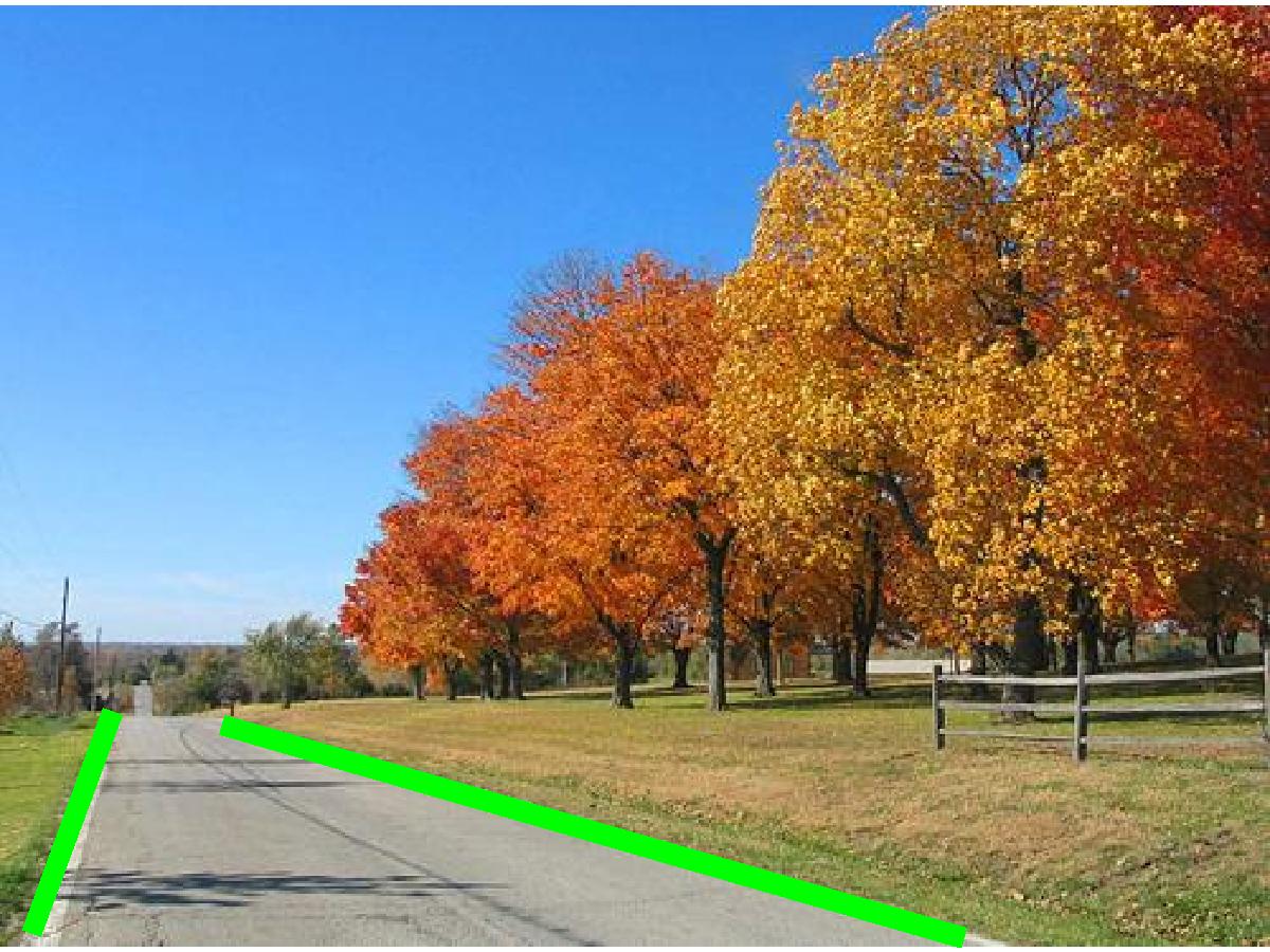
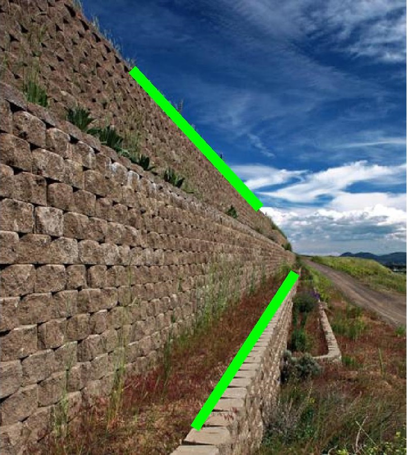
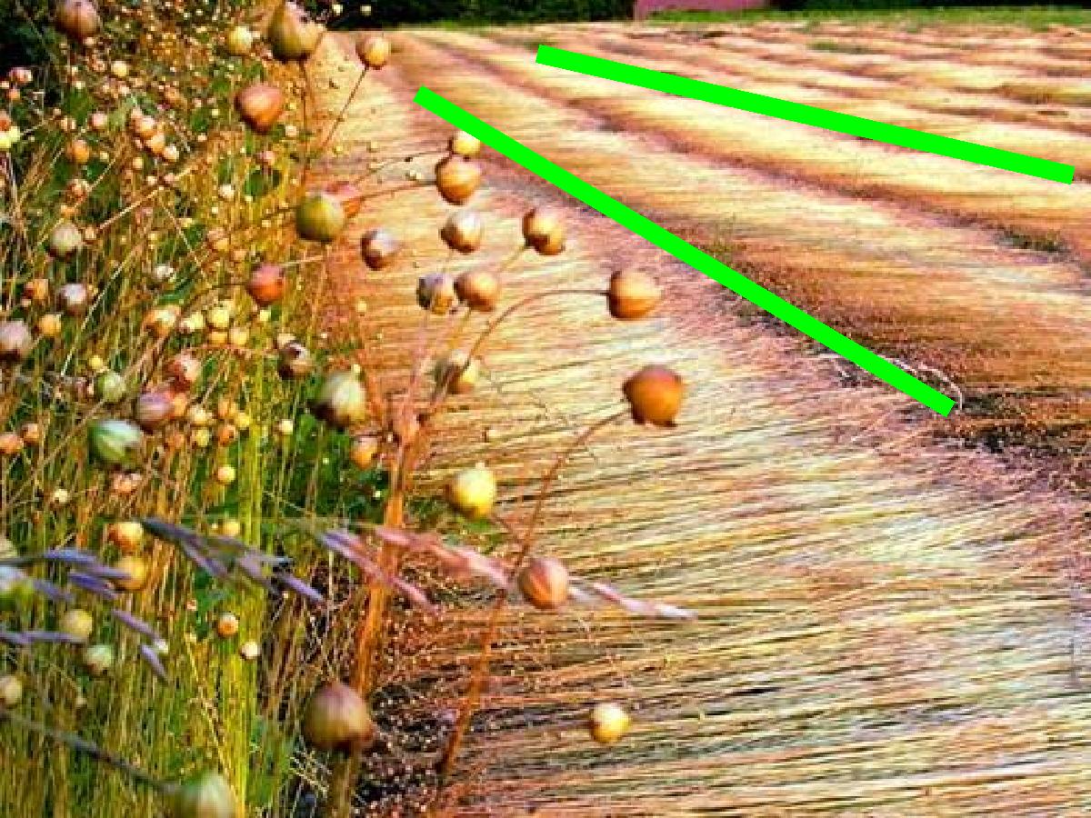
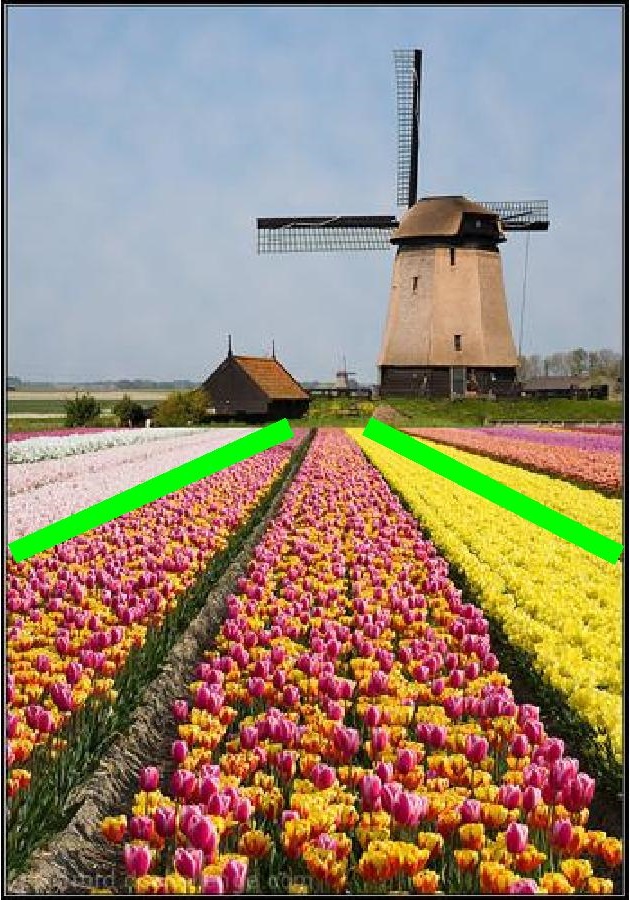
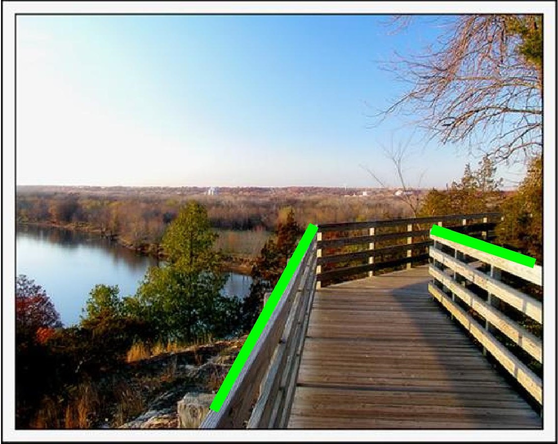
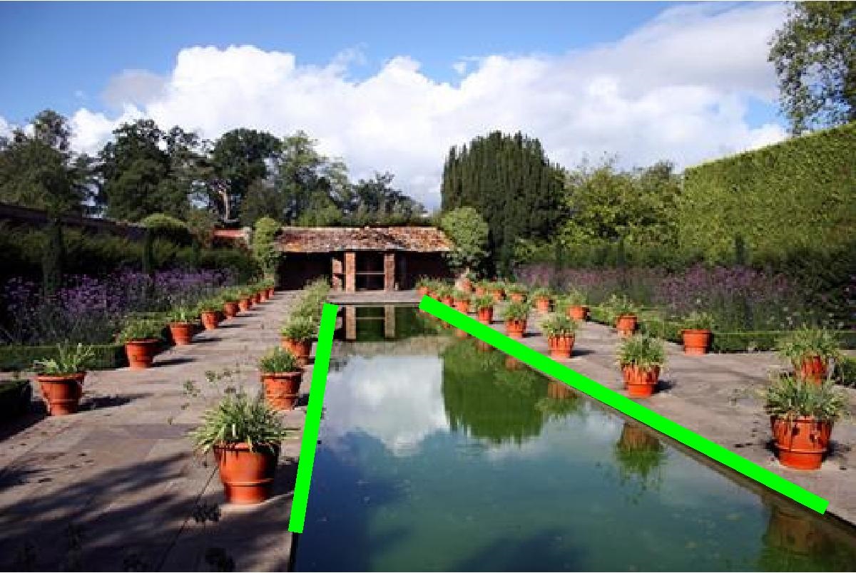
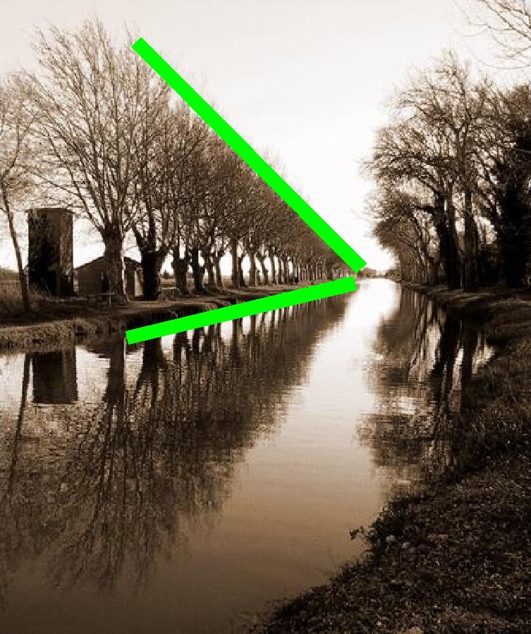
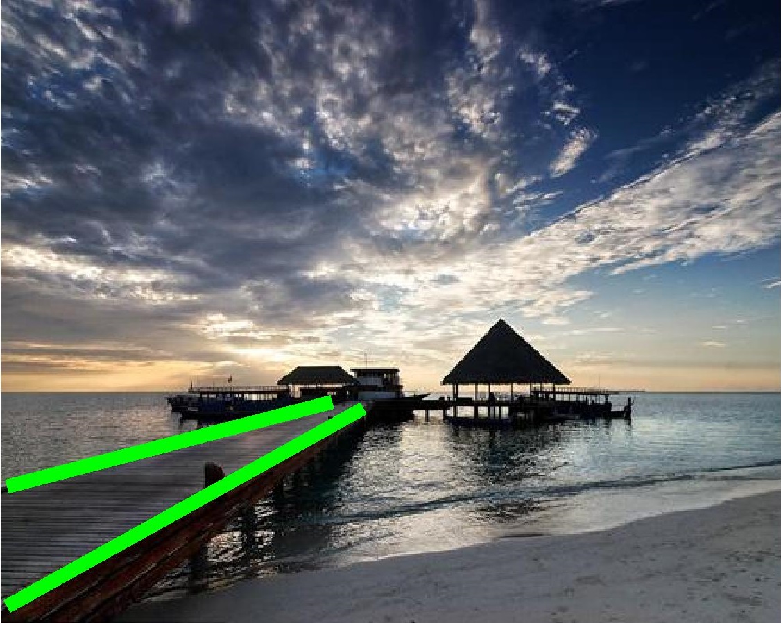
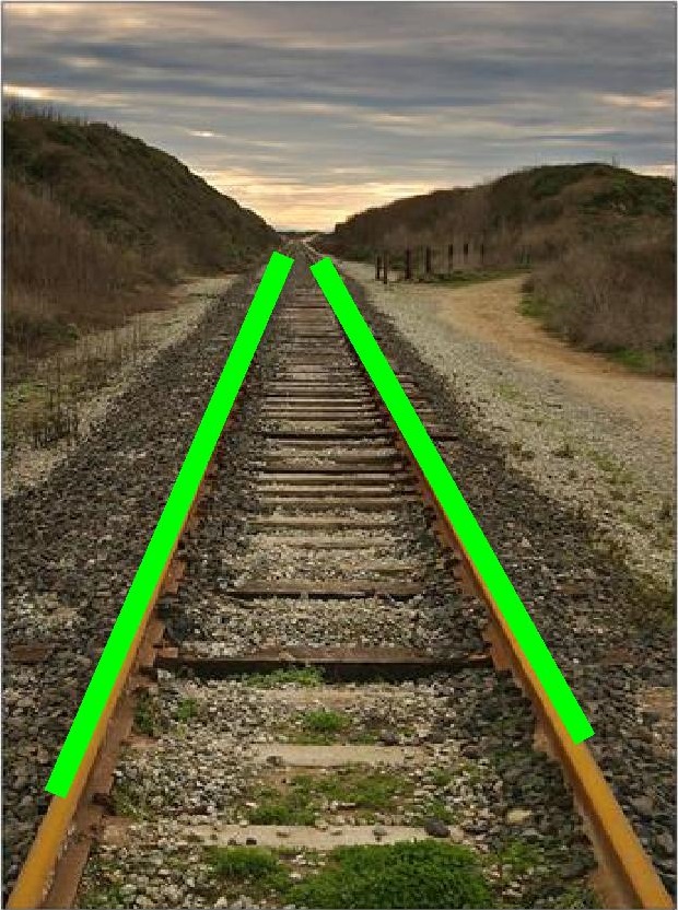
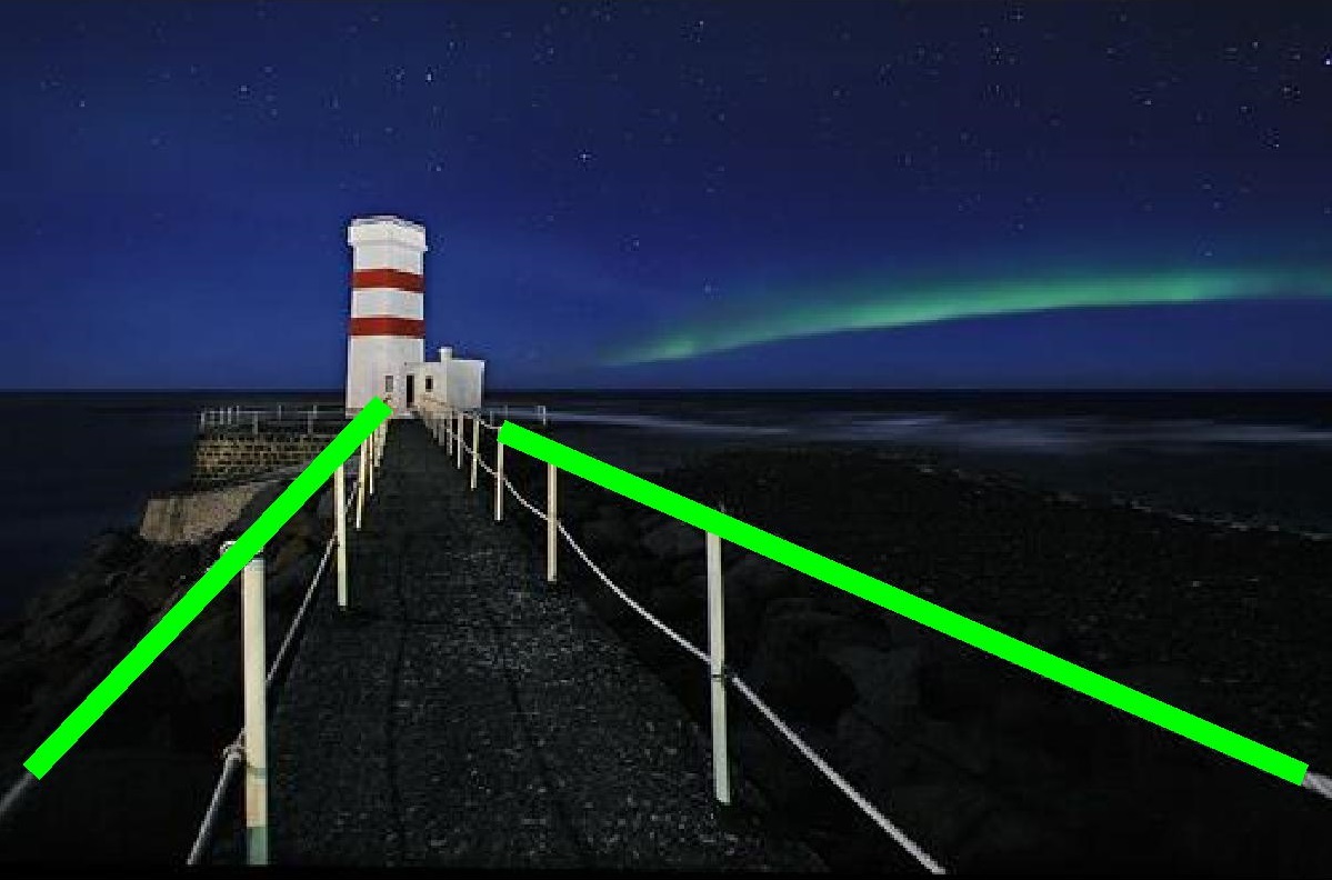
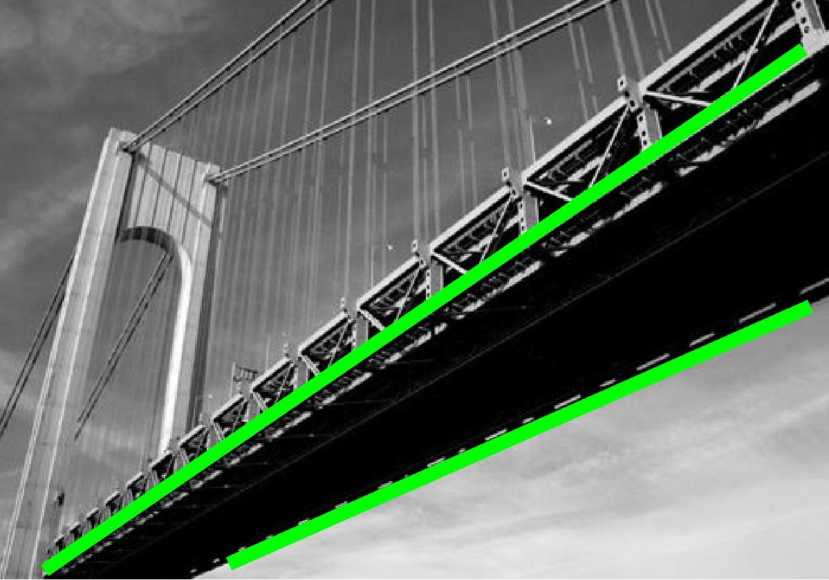
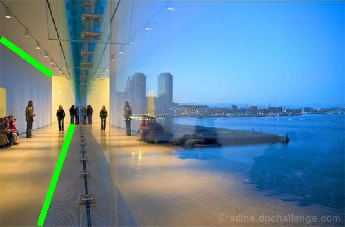
Figure 1: Natural scene images with dominant vanishing points. Images are from the “landscape” category of the AVA dataset. Manually labeled ground truth lines are marked in green.

However, little attention has been paid to natural landscape scenes – a significant genre in both professional and consumer photography. Known as an effective tool in recognizing the viewer as a specific unique individual in a distinct place with a point of view [12], linear perspective has been widely used in natural landscape photography. To bridge this gap between man-made environments and natural landscapes, we conduct a systematical study on the use of linear perspective in such scenes through the detection of the dominant vanishing point in the image. Specifically, we regard a VP in the image the dominant VP if it (i) associates with the major geometric structures (e.g., roads, bridges) of the scene, and (ii) conveys a strong impression of 3D space or depth to the viewers. As illustrated in Figure 1, the dominant VP provides us with important cues about the scene geometry as well as the overall composition of the image.

In natural scene images, a VP is detectable when there are as few as two parallel lines in space. While human eyes have little difficulty identifying the VPs in these images, automatic detection of VPs poses a great challenge to computer systems for two main reasons. First, the visible edges can be weak and not detectable via local photometric cues. Existing line segment detection methods typically assume the gradient magnitude of an edge pixel to be above a certain threshold (e.g., Canny edge detector [13]) or the number of pixels with aligned gradient orientations to be above a certain threshold (e.g., LSD [14]). However, determining the threshold can be difficult due to the weak edges and image noise. Second, the number of edges converging to the VP may be small compared to irrelevant edges in the same scene. As a result, even if a computer system can detect the converging edges, clustering them into one group can be demanding due to the large number of outliers.

To overcome these problems, we propose the use of image contours to detect edges in natural images. Compared to local edge detectors, image contours encode valuable global information about the scene, and thus they are more effective in recognizing weak edges while reducing the number of false detections due to textures. By combining the contour-based edge detection with J-Linkage [15], a popular multi-model detection algorithm, our method significantly outperforms state-of-the-art methods on detecting the dominant VP in natural scene images.

As an application of our VP detection method, we demonstrate how the detected VPs can be used to improve the usefulness of existing content-based image retrieval systems in providing on-site feedback to amateur photographers. Specifically, given a photo taken by the user, we study the problem of finding photos about similar scenes and with similar viewpoints in a large collection of photos. As these photos demonstrate, the use of various photographic techniques, in a situation similar to the one that the user is currently engaged in, could potentially provide effective guidance to the user on his or her own work. Further, in this task, we are also the first to answer an important yet largely unexplored question in the literature: How to determine whether there exists a dominant VP in a photo? To this end, we design a new measure of strength for a given candidate VP, and systematically examine its effectiveness on our dataset.

In summary, the main contributions are as follows:

• We propose the research problem of detecting VPs in natural landscape scenes and a new method for dominant VP detection. By combining a contour-based edge detector with J-Linkage, our method significantly outperforms state-of-the-art methods for natural scenes.

• We develop a new strength measure for VPs and demonstrate its effectiveness in identifying images with a dominant VP.

• We demonstrate the application of our method for assisting amateur photographers at the point of photographic creation via viewpoint-specific image retrieval.

• To facilitate future research, we have created and made available two manually labeled datasets for dominant VPs in 2,275 real-world natural scene images.

II Related Work

II-A Vanishing Point Detection

Vanishing point detection has long been an active research topic in computer vision with many real-world applications such as camera calibration [16, 17], pose estimation [18, 19, 20], height measurement [21], object detection [22], and 3D reconstruction [23, 24]. Since the VPs can be represented by normalized 2D homogeneous coordinates on a Gaussian sphere, early works on VP detection use a Hough transform of the line segments on the Gaussian sphere [25, 26, 27, 28] or a cube map [29]. However, researchers have criticized these methods as being unreliable in the presence of noise and outliers and as having the potential to lead to spurious detections [30]. To reduce spurious responses, Rother [31] enforces the orthogonality of multiple VPs via an exhaustive search, but this process is computationally expensive and requires a criterion to distinguish finite from infinite vanishing points. Alternatively, the Helmholtz principle has been employed to reduce the number of false alarms and reach a high precision level [32].

In [18], Antone and Teller propose an Expectation-Maximization (EM) scheme for VP detection, which is later extended to handle uncalibrated cameras [19, 33]. The EM method iteratively estimates the probability that a line segment belongs to each parallel line groups or an outlier group (E-step) and refines the VPs according to the line segment groups (M-step). The approach, however, requires a good initialization of the vanishing points, which is often obtained by Hough transform or clustering of edges based on their orientations [34].

More recent VP detection algorithms use RANSAC-like algorithms to generate VP hypotheses by computing the intersections of line segments and then select the most probable ones using image-based consistency metrics [7, 8]. In [10], Xu et al. studied various consistency measures between the VPs and line segments and developed a new method that minimizes the uncertainty of the estimated VPs. Lezama et al. [11] proposed to find the VPs via point alignments based on the a contrario methodology. Instead of using edges, Vedaldi and Zisserman proposed to detect VPs by aligning self-similar structures [35]. Zhai et al. [36] used global image context extracted from a deep convolutional network to guide the search for VPs. As we discussed before, these methods are designed for man-made environments. Identifying and clustering edges for VP detection in natural scene images remain a challenging problem.

In addition, there is an increasing interest in exploiting special scene structures for VP detection lately. For example, many methods assume the “Manhattan World” model [37, 20], indicating that three orthogonal parallel-line clusters are present [38, 39, 9, 40]. When the assumption holds, it is shown to improve the VP detection results. Unfortunately, such an assumption is invalid for typical natural scenes. Other related efforts detect VPs in specific scenes such as unstructured roads [41, 42, 43], but how these methods can be extended to general natural scenes remains unclear.

II-B Photo Composition Modeling

Photo composition, which describes the placement or arrangement of visual elements or objects within the frame, has long been a subject of study in computational photography. A line of work has addressed known photographic rules and design principles, such as simplicity, depth of field, golden ratio, rule of thirds, and visual balance. Based on these rules, various image retargeting and recomposition tools have been proposed to improve the image quality [2, 3, 44, 45]. We refer readers to [46] for a comprehensive survey on this topic. However, the use of linear perspective has largely been ignored in the existing work. Compared to the aforementioned rules, which mainly focus on the 2D rendering of visual elements, linear perspective enables photographers to convey the sense of 3D space to the viewers.

Recently, data-driven approaches to composition modeling have gained increasing attention in the multimedia community. These methods use community-contributed photos to automatically learn composition models from the data. For example, Yan et al. [47] propose a set of composition features and learn a model for automatic removal of distracting content and enhancement of the overall composition. In [48], a unified photo enhancement framework is proposed based on the discovery and modeling of aesthetic communities on Flickr. Besides offline image enhancement, composition models learned from exemplar photos can also been used to provide online aesthetics guidance to the photographers, such as selecting the best view [49, 5], recommending the locations and poses of human subjects in a photograph [50, 51, 52], and suggesting the appropriate camera parameters (e.g., aperture, ISO, and exposure) [53]. Our work also takes advantage of vast data available through photo sharing websites. Unlike existing work that each focuses on certain specific aspects of the photo, however, we take a completely different approach to on-site feedback and aim to provide comprehensive photographic guidance through a novel composition-sensitive image retrieval system.

II-C Image Retrieval

The classic approaches to content-based image retrieval [54] typically measure the visual similarity based on low-level features (e.g., color, texture, and shape). Recently, thanks to the availability of large-scale image datasets and computing resources, complicated models have been trained to capture the high-level semantics about the scene [55, 56, 57, 58]. However, because many visual descriptors are generated by local feature extraction processes, the overall spatial composition of the image (i.e., from which viewpoint the image is taken) is usually neglected. To remedy this issue, [4] first classifies images into pre-defined composition categories such as “horizontal”, “vertical”, and “diagonal”. Similar to our work, [59] also explores the VPs in the image for retrieval, but it assumes known VP locations in all images, and thus cannot be applied to a general image database where the majority of the images do not contain a VP. Further, [59] does not consider image semantics for retrieval, hence its usage can be limited in practice.

III Ground Truth Dataset

To create our ground truth datasets, we leverage both the open AVA dataset [60] and the online photo-sharing website Flickr. We have made our datasets publicly available. Below we describe them in detail.

AVA landscape dataset. The original AVA dataset contains over 250,000 images along with a variety of annotations. The dataset provides semantic tags describing the semantics of the images for over 60 categories, such as “natural”, “landscape”, “macro”, and “urban”. For this work, we used the 21,982 images under the category “landscape”.

For each image, we need to determine whether it contains a dominant VP and, if so, label its location. Note that our ground truth data is quite different from those in existing datasets such as York Urban Dataset (YUD) [20] and Eurasian Cities Dataset (ECD) [8]. While these datasets are focused on urban scenes and attempt to identify all VPs in each image, our goal is to identify a single dominant VP associated with the main structures in a wide variety of scenes. The ability to identify the dominant VP in a scene is critical in our targeted applications related to aesthetics and photo composition.

Like existing datasets, we label the dominant VP by manually specifying at least two parallel lines in the image, denoted as $\mathbf{l}_{1}$ and $\mathbf{l}_{2}$ (see Figure 1). The dominant VP location is then computed as $\mathbf{v}=\mathbf{l}_{1}\times\mathbf{l}_{2}$. Because our goal is to identify the dominant VPs only, we make a few assumptions during the process. First, each VP must correspond to at least two visible parallel lines in the image. This assumption eliminates other types of perspective in photography such as diminishing perspective, which is formed by placing identical or similar objects at different distances. Second, for a VP to be the dominant VP in an image, it must correspond to some major structures of the scene and clearly carries more visual weight than other candidates, if any. We do not consider images with two or more VPs carrying similar visual importance, which are typically seen in urban scenes. Similarly, we also exclude images where it is impossible to determine a single dominant direction due to parallel curves (Figure 2). Finally, observing that only those VPs which lie within or near the image frame convey a strong sense of perspective to the viewers, we resize each image so that the length of its longer side is 500 pixels, keeping only the dominant VPs that lie within a $1,000\times 1,000$ frame, with the image placed at the center. We used the size $500$ pixels as a trade-off between keeping details and providing fast runtime for large-scale applications.

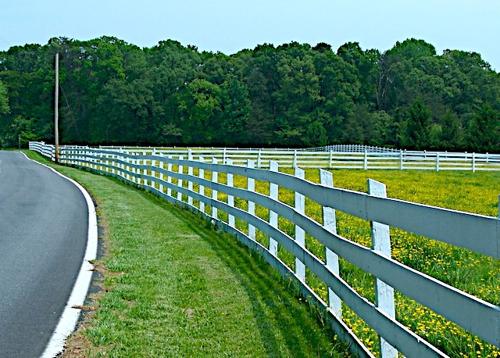
Figure 2: Example natural scene images that are not suitable for this work. The first two images show diminishing perspective. The third image has two VPs. The last image contains parallel curves, not parallel lines.

We collected a total of 1,316 images with annotations of ground truth parallel lines.

Flickr dataset. To test the generality of our VP detection method, we have also downloaded images from Flickr by querying the keyword “vanishing point”. These images cover a wide variety of scenes from nature, rural, and travel to street and cityscape. Following the same procedure above, for each image, we determine whether it contains a dominant VP and, if so, label its location. We only keep the images with a dominant VP. This step results in a dataset consisting of 959 annotated images.

IV Contour-based Vanishing Point Detection for Natural Scenes

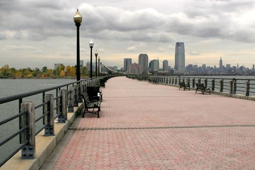
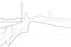
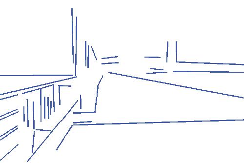
(a)	(b)	(c)

Figure 3: Contour-based edge detection. (a) Original image. (b) The ultrametric contour map (UCM). (c) Filtered edges.

Given a set of edges $\mathcal{E}=\{E_{1},\ldots,E_{N}\}$, a VP detection method aims to classify the edges into several classes, one for each VP in the scene, plus an “outlier” class. Similar to [7], we employ the J-Linkage algorithm [15] for multiple model estimation and classification. The most important new idea of our method lies in the use of contours to generate the input edges. As we will see in this section, our contour-based method can effectively identify weak edges in natural scene images and reduce the number of outliers at the same time, leading to significantly higher VP detection accuracy.

IV-A Edge Detection via Contours

Because we rely on edges to identify the dominant VP in an image, an ideal edge detection method should have the following properties: (i) it should detect all edges that converge to the true VPs, (ii) the detected edges should be as complete as possible, and (iii) it should minimize the number of irrelevant or cluttered edges. Unfortunately, local edge-detection methods do not meet these criteria. A successful method must go beyond local measurements and utilize global visual information.

Our key insight is that in order to determine if an edge is present at a certain location, it is necessary to examine the relevant regions associated with it. This assertion is motivated by observing that humans label the edges by first identifying the physical objects in an image. In addition, based on the level of details they choose, different people may make different decisions on whether to label a particular edge.

Accordingly, for edge detection, we employ the widely-used contour detection method [61], which proposed a unified framework for contour detection and image segmentation using an agglomerative region clustering scheme. In the following, we first discuss the main difference between the contours and edges detected by local methods before showing how to obtain straight edges from the contours.

Globalization in contour detection. Comparing to the local methods, the contours detected by [61] enjoy two levels of globalization.

First, as a global formulation, spectral clustering has been widely used in image segmentation to suppress noise and boost weak edges. Generally, let $W$ be an affinity matrix whose entries encode the (local) similarity between pixels, this method solves for the generalized eigenvectors of the linear system: $(D-W)\mathbf{v}=\lambda D\mathbf{v}$, where the diagonal matrix $D$ is defined as $D_{ii}=\sum_{j}W_{ij}$. Let $\{\mathbf{v}_{0},\mathbf{v}_{1},\ldots,\mathbf{v}_{K}\}$ be the eigenvectors corresponding the $K+1$ smallest eigenvalues $0=\lambda_{0}\leq\lambda_{1}\leq\cdots\leq\lambda_{K}$. Using all the eigenvectors except $\mathbf{v}_{0}$, one can then represent each image pixel with a vector in $\mathbb{R}^{K}$. As shown in [61], the distances between these new vectors provide a denoised version of the original affinities, making them much easier to cluster.

Second, a graph-based hierarchical clustering algorithm is used in [61] to construct an ultrametric contour map (UCM) of the image (see Figure 3(b)). The UCM defines a duality between closed, non-self-intersecting weighted contours and a hierarchy of regions, where different levels of the hierarchy correspond to different levels of detail in the image. Thus, each weighted contour in UCM represents the dissimilarity of two, possibly large, regions in the image, rather than the local contrast of small patches.

From contours to edges. Let $\mathcal{C}=\{C_{1},C_{2},\ldots\}$ denote the set of all weighted contours. To recover straight edges from the contour map, we apply a scale-invariant contour subdivision procedure. Specifically, for any contour $C_{j}$, let $\mathbf{c}_{j}^{1}$ and $\mathbf{c}_{j}^{2}$ be the two endpoints of $C_{j}$, we first find the point on $C_{j}$ which has the maximum distance to the straight line segment connecting its endpoints:

$$\mathbf{p}^{*}=\arg\max_{\mathbf{p}\in C_{j}}dist(\mathbf{p},\overline{\mathbf{c}_{j}^{1}\mathbf{c}_{j}^{2}})\;.$$ (1)

We then subdivide $C_{j}$ at $\mathbf{p}^{*}$ if the maximum distance is greater than a fixed fraction $\alpha$ of the contour length:

$$dist(\mathbf{p}^{*},\overline{\mathbf{c}_{j}^{1}\mathbf{c}_{j}^{2}})>\alpha\cdot|C_{j}|\;.$$ (2)

By recursively applying the above procedure to all the contours, we obtain a set of approximately straight edges $\mathcal{E}=\{E_{1},\ldots,E_{N}\}$. We only keep edges that are longer than certain threshold $l_{\min}$, because short edges are very sensitive to image noises (Figure 3(c)).

Quantitative evaluation. We compare the performance of our contour-based edge detection to two popular edge detectors: the Canny detector [13] and the Line Segment Detector (LSD) [14]. For this experiment, we have randomly chosen 100 images from our AVA landscape dataset and manually labeled all the edges that converge to the dominant VP in each image. With the ground truth edges, all methods are then evaluated quantitatively by means of the recall and precision as described in [62]. Here, recall is the fraction of true edge pixels that are detected, whereas precision is the fraction of edge pixel detections that are indeed true positives (i.e., those consistent with the dominant VP). Note that in the context of edge detection, the particular measures of recall and precision allow for some small tolerance in the localization of the edges (see [62] for details).

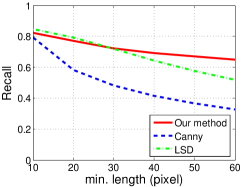
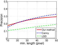
(a) Recall	(b) Precision

Figure 4: Quantitative evaluation of edge detection methods.

In Figure 4, we report the recall and precision of all methods as a function of the minimum edge length $l_{\min}$. Since most VP detection methods rely on clustering the detected edges, an ideal edge detector should maximize the number of edges consistent with the ground truth dominant VP and and minimize the number of irrelevant edges. Thus, higher recall and precision indicate better performance. As shown in Figure 4, compared to LSD, our method achieves comparable recall but with much higher precision. Meanwhile, while Canny has similar precision as our method, its recall is substantially lower. This result is expected as Canny operates on pixels with high gradient values, but such pixels are often absent in natural scenes (i.e., low recall). While LSD is able to overcome this difficulty and achieve higher recall by computing the statistics in surrounding rectangular regions instead, the ambiguity in the region size often leads to repeated detections (i.e., low precision). Thus, our contour-based method is an overall better choice for the vanishing point detection task.

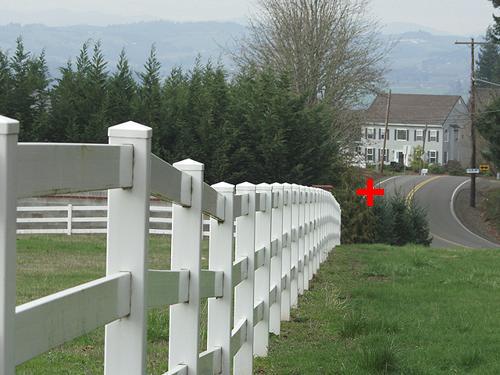
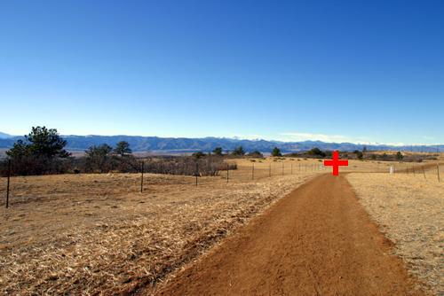
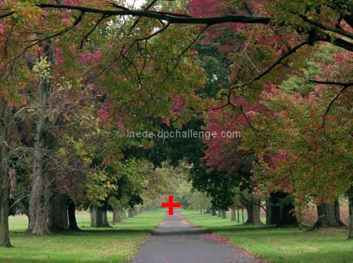
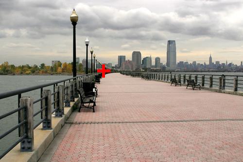
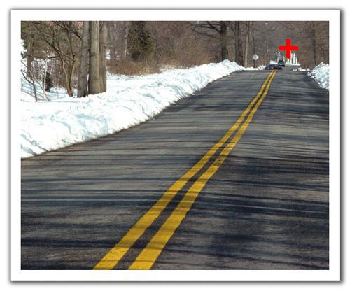
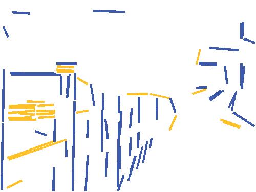
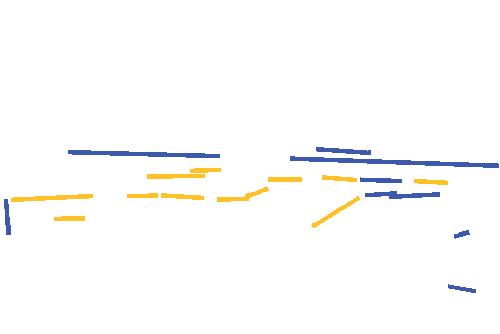
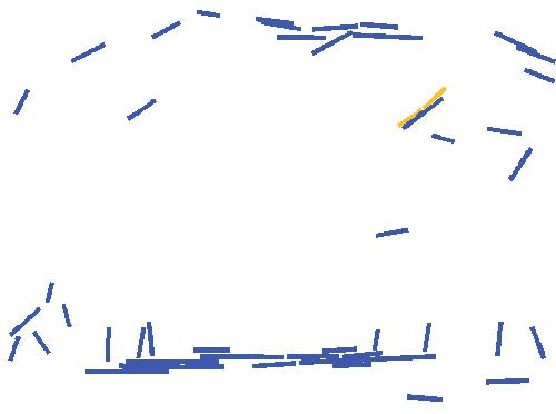
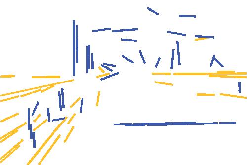
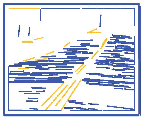
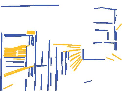
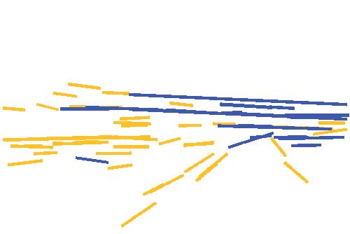
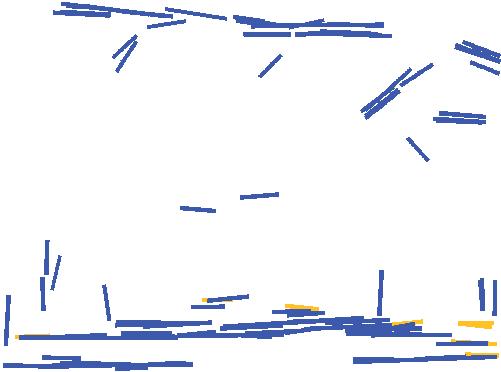
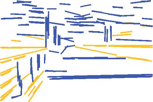
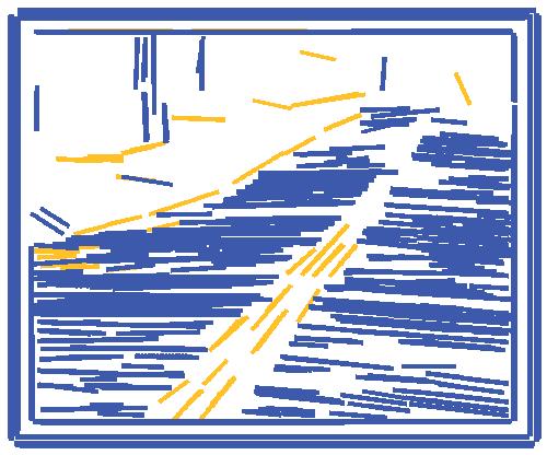
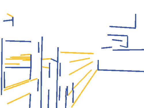
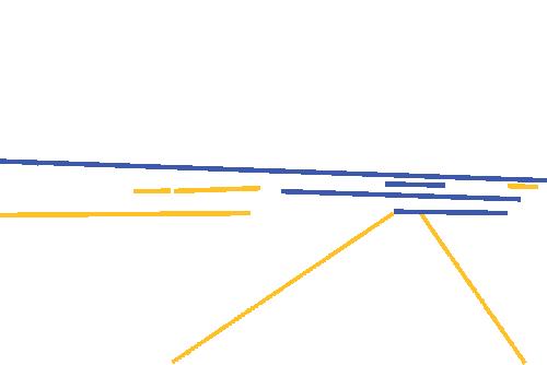
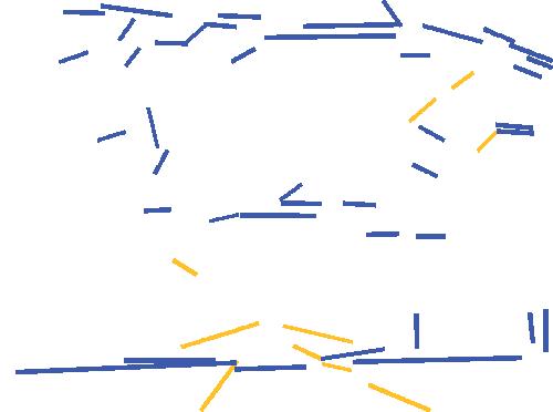
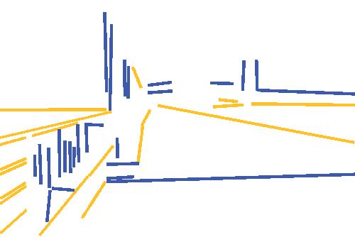
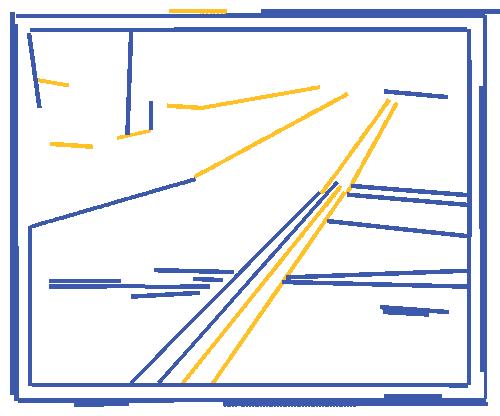
(a)                          (b)                          (c)                          (d)                         (e)

Figure 5: Example detections of different edge detection methods. The four rows show the original images, and the edges detected by Canny detector, LSD, and our contour-based method, respectively. Yellow edges indicate the edges consistent with the ground truth dominant VP.

In Figure 5, we further show some example edge detection results. As shown, our contour-based method can better detect weak yet important edges in terms of both the quantity and the completeness. For example, our method is able to detect the complete edges of the road in Figure 5(b), while the local methods only detected parts of them. Also, only our method successfully detected the edges of the road in Figure 5(c).

Another important distinction between our contour-based method and the local methods concerns the textured areas in the image. Local methods tend to confuse image texture with true edges, resulting in a large number of detections in these areas (e.g., the sky region and the road in 5(d) and (e), respectively). Such false positives often lead to incorrect clustering results in the subsequent VP detection stage. Meanwhile, our method treats the textured area as a whole, thereby greatly reducing the number of false positives.

IV-B J-Linkage

In this section, we give an overview of the J-Linkage algorithm [15]. Similar to RANSAC, J-Linkage first randomly chooses $M$ minimal sample sets and computes a putative model for each of them. For VP detection, the $j$-th minimal set consists of two randomly chosen edges: $(E_{j_{1}},E_{j_{2}})$. To this end, we first fit a line $\mathbf{l}_{i}$ to each edge $E_{j}\in\mathcal{E}$ using least squares. Then, we can generate the hypothesis $\mathbf{v}_{j}$ using the corresponding fitted lines: $\mathbf{v}_{j}=\mathbf{l}_{j_{1}}\times\mathbf{l}_{j_{2}}$ .

Next, J-Linkage constructs a $N\times M$ preference matrix $P$, where the $(i,j)$-th entry is defined as:

$$p_{ij}=\left\{\begin{array}[]{ll}1&\textup{if }D(E_{i},\mathbf{v}_{j})\leq\phi\\ 0&\textup{otherwise}\end{array}\right.\;.$$ (3)

Here, $D(E_{i},\mathbf{v}_{j})$ is a measure of consistency between edge $E_{i}$ and VP hypothesis $\mathbf{v}_{j}$, and $\phi$ is a threshold. Note that $i$-th row indicates the set of hypotheses edge $E_{i}$ has given consensus to, and is called the preference set (PS) of $E_{i}$. J-Linkage then uses a bottom-up scheme to iteratively group edges that have similar PS. Here, the PS of a cluster is defined as the intersection of the preference sets of its members. In each iteration, the two clusters with the smallest distance are merged, where the Jaccard distance is used to measure the similarity between any two clusters $A$ and $B$:

$$d_{J}(A,B)=\frac{|A\bigcup B|-|A\bigcap B|}{|A\bigcup B|}\;.$$ (4)

The operation is repeated until the distance between any two clusters is 1.

Consistency measure. We intuitively define the consistency measure $D(E_{i},\mathbf{v}_{j})$ as the root mean square (RMS) distance from all points on $E_{i}$ to a line $\hat{\mathbf{l}}$, such that $\hat{\mathbf{l}}$ passes through $\mathbf{v}_{j}$ and minimizes the distance:

$$D_{RMS}(E_{i},\mathbf{v}_{j})=\min_{l:l\times\mathbf{v}_{j}=0}\left(\frac{1}{N}\sum_{\mathbf{p}\in E_{i}}dist(\mathbf{p},\mathbf{l})^{2}\right)^{\frac{1}{2}}\;,$$ (5)

where $N$ is the number of points on $E_{i}$, and $dist(\mathbf{p},\l)$ is the perpendicular distance from a point $\mathbf{p}$ to a line $\l$, i.e., the length of the line segment which joins $\mathbf{p}$ to $\l$ and is perpendicular to $\l$.

IV-C Experiments

In this section, we present a comprehensive performance study of our contour-based VP detection method and compare it to the state-of-the-art methods. We use both the AVA landscape dataset and the Flickr dataset described in Section III. Similar to previous work (e.g., [7, 9]), we evaluate the performance of a VP detection method based on the consistency of the ground truth edges with the estimated VPs. Specifically, let $\{E_{k}^{G}\}_{k=1}^{K}$ be the set of ground truth edges, the consistency error of a detection $\hat{\mathbf{v}}$ is:

$$err(\hat{\mathbf{v}})=\frac{1}{K}\sum_{k}D_{RMS}(E_{k}^{G},\hat{\mathbf{v}})\;.$$ (6)

For all experiments, we compute the average consistency error over five independent trials.

IV-C1 Dominant Vanishing Point Detection Results

Figure 6 reports the cumulative histograms of vanishing point consistency error w.r.t. the ground truth edges for various methods. Below we analyze the results in detail.

Comparison of edge detection methods. We first compare our method to Canny detector [13] and LSD [14] in terms of the accuracy of the detected VPs. For our contour-based method, the parameters are: $\alpha=0.05$, $l_{\min}=40$, and $\phi=3$. For Canny detector and LSD, we tune the parameters $l_{\min}$ and $\phi$ so that the highest accuracy is obtained. In this experiment, we simply keep the VP with the largest support set as the detection result. Our contour-based method significantly outperforms the other edge detection methods.

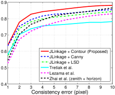
(a) AVA Landscape	(b) Flickr

Figure 6: Dominant vanishing point detection results. We show the cumulative histograms of vanishing point consistency error w.r.t. the ground truth edges (Eq. (6)) for all candidate methods.

Comparison with the state-of-the-art. We also compare our method to state-of-the-art VP detection methods. As we discussed before, most existing methods focus on urban scenes and make strong assumptions about the scene structures, such as a Manhattan world model [38, 39, 9, 40]. Such strong assumptions render these methods inapplicable to natural landscape scenes.

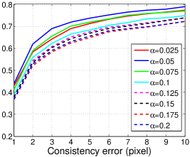
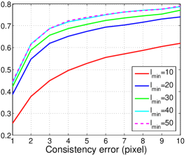
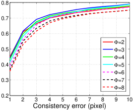
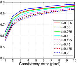
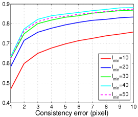
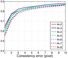
(a) $\alpha$	(b) $l_{\min}$	(c) $\phi$

Figure 7: Accuracy of our method w.r.t. parameters. First row: AVA landscape dataset. Second row: Flickr dataset.

While other methods do not explicitly assume a specific model, they still benefit from the scene structures to various extents. In Figure 6, we compare our method to three recent methods, namely Tretiak et al. [8], Lezama et al. [11], and Zhai et al. [36]. For each method, we use the source code downloaded from its author’s website. Note that [11] uses the Number of False Alarms (NFA) to measure the importance of the VPs. For fair comparison, we keep the VP with the highest NFA. Further, [36] takes a two-step approach which first detects one zenith VP and then detects the horizontal VPs. As it is unclear from [36] how to compare the strength of zenith VP with the horizontal VPs, we choose to favor [36] in our experiment setting by considering both the zenith VP and the top-ranked horizontal VP in the evaluation and keeping the VP which achieves the smallest consistency error w.r.t. the ground truth edges.

Figure 6 shows that the three methods do not perform well on the natural landscape images. The problem is that [8] assumes multiple horizontal VP detections for horizon and zenith estimation, whereas [36] attempts to detect both zenith and horizontal VPs. However, there may not be more than one VP in natural scenes. Similarly, [11] relies on the multiple horizontal VP detections to filter redundant and spurious VPs.

IV-C2 Parameter Sensitivity

Next, we study the performance of our contour-based VP detection method w.r.t. the parameters $\alpha$, the minimum edge length $l_{\min}$, and the distance threshold $\phi$ in Eq. (3). We conduct experiments with one of these parameters varying while the others are fixed. The default parameter setting is $\alpha=0.05$, $l_{\min}=40$, and $\phi=3$.

Performance w.r.t. $\alpha$. Recall from Section IV-A that $\alpha$ controls the degree to which a contour segment may deviate from a straight line before it is divided into two sub-segments. Figure 7(a) shows that the best performance is achieved with $\alpha=0.05$.

Performance w.r.t. minimum edge length $l_{\min}$. Figure 7(b) shows the performance of our method as a function of $l_{\min}$. Rather surprisingly, we find that the accuracy is quite sensitive to $l_{\min}$. This finding probably reflects the relatively small number of edges consistent with the dominant VP available in natural scenes. Therefore, if $l_{\min}$ is too small, these edges may be dominated by irrelevant edges in the scene; if $l_{\min}$ is too large, there may not be enough inliers to robustly estimate the VP location.

Performance w.r.t. threshold $\phi$. Figure 7(c) shows the accuracy of our method w.r.t. the threshold $\phi$ in Eq. (3). As shown, our method is relatively insensitive to the threshold, and achieves the best performance when $\phi=3$.

Finally, we note that the experiment results are very consistent across the two different datasets. This finding suggests that the choice of the parameters is insensitive to the datasets and can be well extrapolated to general images.

V Selection of the Dominant Vanishing Point

In real-world applications concerning natural scene photos, it is often necessary to select the images in which a dominant VP is present since many images do not have a VP. Further, if multiple VPs are detected, we need to determine which one carries the most importance in terms of the photo composition. Therefore, given a set of candidates $\{\mathbf{v}_{j}\}_{j=1}^{n}$ generated by a VP detection method, our goal is to find a function $f$ which well estimates the strength of a VP candidate. Then, we can define the dominant VP of an image as the one whose strength is (i) the highest among all candidates, and (ii) higher than certain threshold $T$:

$$\mathbf{v}^{*}=\arg\max_{f(\mathbf{v}_{j})\geq T}f(\mathbf{v}_{j})\;.$$ (7)

In practice, given a detected VP $\mathbf{v}_{j}$ and the edges $\mathcal{E}_{j}\subseteq\mathcal{E}$ associated with the cluster obtained by a clustering method (e.g., J-Linkage), a simple implementation of $f$ would be the number of edges: $f(\mathbf{v}_{j})=|\mathcal{E}_{j}|$. Note that it treats all edges in $\mathcal{E}_{j}$ equally. However, we have found this approach problematic for natural images because it does not consider the implied depth of each edge in the 3D space.

V-A The Strength Measure

Intuitively, an edge conveys a strong sense of depth to the viewers if (i) it is long, and (ii) it is close to the VP (Figure 1). This observation motivates us to examine the implied depth of each individual point on an edge, instead of treating the edge as a whole.

Geometrically, as shown in Figure 8, let $E$ be a line segment consistent with vanishing point $\mathbf{v}=(v_{x},v_{y},1)^{T}$ in the image. We further let $D$ be the direction in 3D space (i.e., a point at infinity) that corresponds to $\mathbf{v}$: $\mathbf{v}=PD$, where $P\in\mathbb{R}^{3\times 4}$ is the camera projection matrix.

Figure 8: Illustration of our edge strength measure.

For any pixel on the line segment $\mathbf{q}=(q_{x},q_{y},1)^{T}\in E$, we denote $Q$ as the corresponding point in the 3D space. Then, we can represent $Q$ as a point on a 3D line with direction $D$: $Q=A+\lambda D$, where $A$ is some reference point chosen on this line, and $\lambda$ can be regarded as the (relative) distance between $A$ and $Q$. Consequently, we have

$$\mathbf{q}=PQ=P(A+\lambda D)=\mathbf{a}+\lambda\mathbf{v}\;,$$ (8)

where $\mathbf{a}=(a_{x},a_{y},1)^{T}$ is the image of $A$. Thus, let $l_{\mathbf{q}}$ and $l_{\mathbf{a}}$ denote the distance on the image from $\mathbf{q}$ and $\mathbf{a}$ to $\mathbf{v}$, respectively, we have

$$\lambda=l_{\mathbf{a}}/l_{\mathbf{q}}-1\;.$$ (9)

Note that if we choose $A$ as the intersecting point of the 3D line corresponding to $E$ and the image plane, $\lambda$ represents the (relative) distance from any point $Q$ on this line to the image plane along direction $D$. In practice, although $l_{\mathbf{a}}$ is typically unknown and varies for each edge $E$, we can still infer from Eq. (9) that $\lambda$ is a linear function of $1/l_{\mathbf{q}}$. This motivates us to define the weight of a pixel $\mathbf{q}\in E$ as $(l_{\mathbf{q}}+\tau)^{-1}$, where $\tau$ is a constant chosen to make it robust to noises and outliers.

Thus, our new measure of strength for $\mathbf{v}_{j}$ is defined as

$$f(\mathbf{v}_{j})=\sum_{E\in\mathcal{E}_{j}}\sum_{\mathbf{q}\in E}\frac{1}{l_{\mathbf{q}}+\tau}\;.$$ (10)

Clearly, edges that are longer and closer to the VP have more weights according to our new measure.

V-B Experiments

Dominant vanishing point selection. We first demonstrate the effectiveness of the proposed strength measure in selecting the dominant VP from the candidates obtained by our VP detection algorithm. In Figure 9, we compare the following three measures in terms of the consistency error of the selected dominant VP:

Edge Num: The number of edges associated with each VP.

Edge Sum: The sum of the edge lengths associated with each VP.

Proposed: Our strength measure Eq. (10).

As shown, by considering the length of an edge and its proximity to the VP, our proposed measure achieves the best performance in selecting the dominant VP in the image.

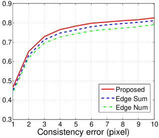
Figure 9: Experiment results on dominant vanishing point selection.

Dominant vanishing point verification. Next, we evaluate the effectiveness of the proposed measure in determining the existence of a dominant VP in the image. For this experiment, we use all the 1,316 images with labeled dominant VPs as positive samples and randomly select 1,500 images without a VP from the “landscape” category of AVA dataset as negative samples. In Figure 10, we plot the ROC curves of the three different measures. As a baseline, we also include the result of the Number of False Alarms (NFA) score proposed in [11], which measures the likelihood that a specific configuration (i.e., a VP) arises from a random image. One can clearly see that our proposed measure achieves the best performance.

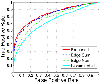
Figure 10: Experiment results on dominant vanishing point verification.

In Figure 11(a) and (b), we further plot the percentage of images and the average consistency error as functions of our strength measure, respectively. In particular, Figure 11(b) shows that the consistency error decreases substantially when the strength score is higher than 150. This outcome suggests that our strength measure is a good indicator of the reliability of a VP detection result.

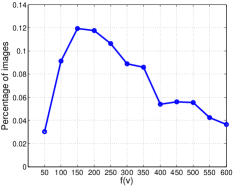
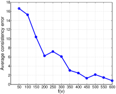
(a)	(b)

Figure 11: The impact of VP strength on the accuracy of dominant VP detection. We show (a) the percentage of images and (b) the average consistency error as a function of our strength measure Eq. (10).

VI Photo Composition Application

In this section, we demonstrate an interesting application of our dominant VP detection method in automatic understanding of photo composition. Nowadays, Cloud-based photo sharing services such as flickr.com, photo.net, and dpchallenge.com have played an increasingly important role in helping the amateurs improve their photography skills. Considering the scenario where a photographer is about to the take a photo of a natural scene, he or she may wonder what photos peers or professional photographers would take in a similar situation. Therefore, given a shot taken by the user, we propose to find exemplar photos about similar scenes with similar points of view in a large collection of photos. These photos demonstrate the use of various photographic techniques in real world scenarios, hence could potentially be used as feedback to the user on his or her own work.

VI-A Viewpoint-Specific Image Retrieval

Given two images $I_{i}$ and $I_{j}$, our similarity measure is a sum of two components:

$$D(I_{i},I_{j})=D_{s}(I_{i},I_{j})+D_{p}(I_{i},I_{j}),$$ (11)

where $D_{s}$ and $D_{p}$ measures the similarity of two images in terms of the scene semantics and the use of linear perspective, respectively. Below we describe each term in detail.

Semantic similarity $D_{s}$: Recently, it has been shown that generic descriptors extracted from the convolutional neural networks (CNNs) are powerful in capturing the image semantics (e.g., scene types, objects) and have been successfully applied to obtain state-of-the-art image retrieval results [58]. In our experiment, we adopt the publicly available CNN model trained by [63] on the ImageNet ILSVRC challenge dataset to compute the semantic similarity. Specifically, we represent each image using the $\ell_{2}$-normalized output of the second fully connected layer (full7 of [63]), and adopt the cosine distance to measure the feature similarity.

Perspective similarity $D_{p}$: To model the perspective effect in the image, we consider two main factors: (i) the location of the dominant VP and (ii) the position of the associated image elements. For the latter, we focus on the edges consistent with the dominant VP obtained via our contour-based VP detection algorithm. Let $\mathbf{v}_{i}$ and $\mathbf{v}_{j}$ be the locations of the dominant VPs in images $I_{i}$ and $I_{j}$, respectively. We use $\mathcal{E}_{i}$ (or $\mathcal{E}_{j}$) to denote the sets of edges consistent with $\mathbf{v}_{i}$ (or $\mathbf{v}_{j}$). Our perspective similarity measure is defined as:

$$D_{p}(I_{i},I_{j})=\gamma_{1}\max\left(1-\frac{\|\mathbf{v}_{i}-\mathbf{v}_{j}\|}{len},0\right)+\gamma_{2}K(\mathcal{E}_{i},\mathcal{E}_{j})\;,$$ (12)

where $\|\mathbf{v}_{i}-\mathbf{v}_{j}\|$ is the Euclidean distance between $\mathbf{v}_{i}$ and $\mathbf{v}_{j}$, $len$ is the length of the longer side of the image. We resize all the images to $len=500$.

Further, since each edge can be regarded as a set of 2D points on the image, $K(\mathcal{E}_{i},\mathcal{E}_{j})$ should measure the similarity of two point sets. Here, we use the popular spatial pyramid matching [64] for its simplicity and efficiency. Generally speaking, this matching scheme is based on a series of increasingly coarser grids on the image. At any fixed resolution, two points are said to match if they fall into the same grid cell. The final matching score is a weighted sum of the number of matches that occur at each level of resolution, where matches found at finer resolutions have higher weights than do matches found at coarser resolutions.

For our problem, we first construct a series of grids at resolutions $0,1,\ldots,L$, as illustrated in Figure 12. Note that the grid at level $l$ has $2^{l}$ cells along each dimension, so the total number of cells is $2^{2l}$. At level $l$, let $H_{i}^{l}(k)$ and $H_{j}^{l}(k)$ denote the number of points from $\mathcal{E}_{i}$ and $\mathcal{E}_{j}$ that fall into the $k$-th cell, respectively. The number of matches at level $l$ is then given by the histogram intersection function:

$$\mathcal{I}(H_{i}^{l},H_{j}^{l})=\sum_{k}\min\left(H_{i}^{l}(k),H_{j}^{l}(k)\right)\;.$$ (13)

Below we write $\mathcal{I}(H_{i}^{l},H_{j}^{l})$ as $\mathcal{I}^{l}$ for short.

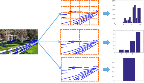
Figure 12: Illustration of the construction of a three-level spatial pyramid. Given the set of edges $\mathcal{E}_{i}$ consistent with the dominant VP, we subdivide the image at three different level of resolutions. For each resolution, we count the number of edge points that fall into each bin to build the histograms $H_{i}^{l},l=0,1,2$.

Since the number of matches found at level $l$ also includes all the matches found at the level $l+1$, the number of new matches at level $l$ is given by $\mathcal{I}^{l}-\mathcal{I}^{l+1}$, $\forall l=0,\ldots,l-1$. To reward matches found at finer levels, we assign weight $2^{-(L-l)}$ to the matches at level $l$. Note that the weight is inversely proportional to the cell width at that level. Finally, the pyramid matching score is defined as:

$$K^{L}(\mathcal{E}_{i},\mathcal{E}_{j}) = \mathcal{I}^{L}+\sum_{l=0}^{L-1}\frac{1}{2^{L-l}}(\mathcal{I}^{l}-\mathcal{I}^{l+1})$$ (14)

$$= \frac{1}{2^{L}}\mathcal{I}^{0}+\sum_{l=1}^{L}\frac{1}{2^{L-l+1}}\mathcal{I}^{l}\;.$$ (15)

Here, we use superscript “$L$” to indicate its dependency on the parameter $L$. We empirically set the parameters for viewpoint-specific image retrieval for all experiments to: $\gamma_{1}=\gamma_{2}=0.5,L=6$.

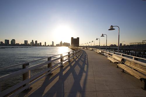
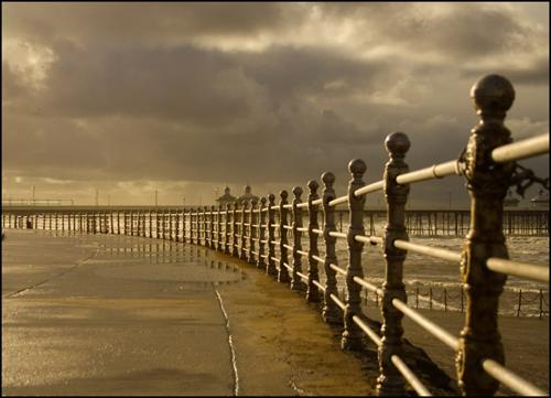
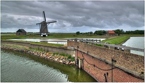
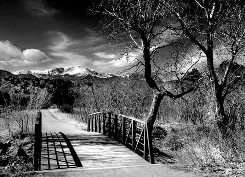
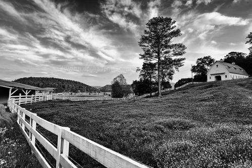
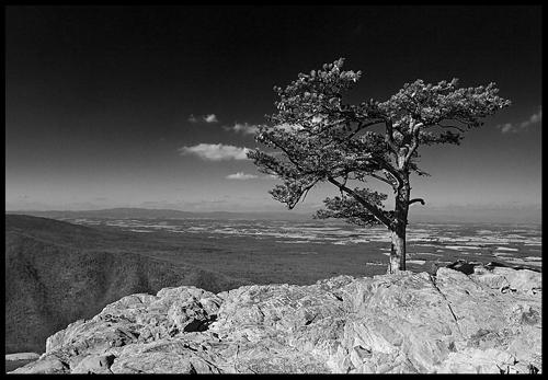
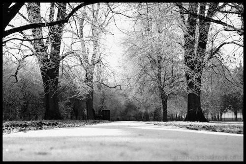
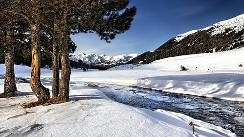
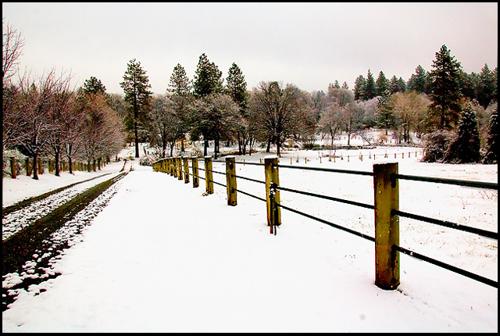
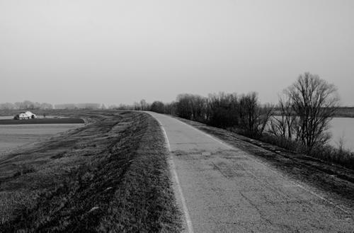
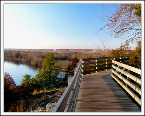
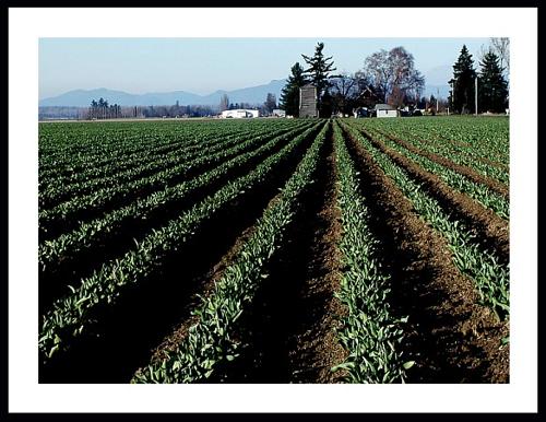
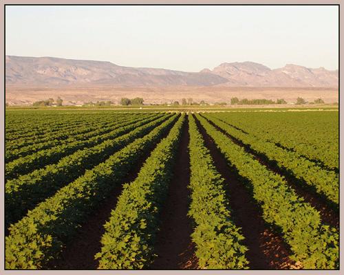
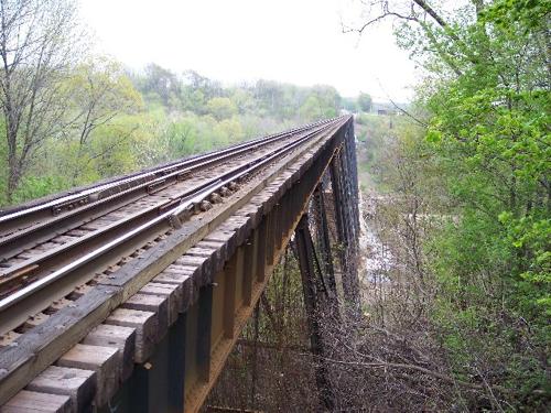
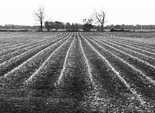
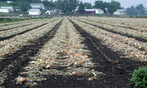
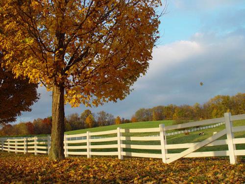
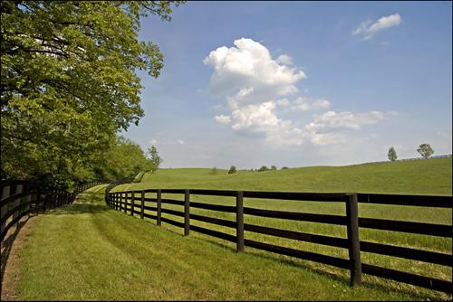
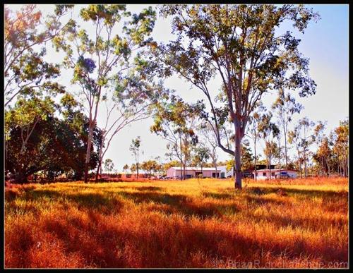
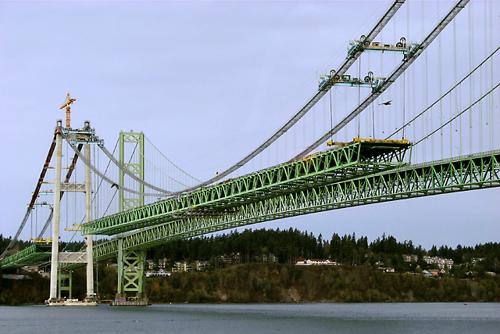
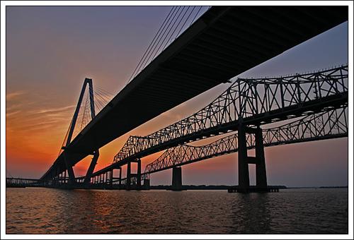
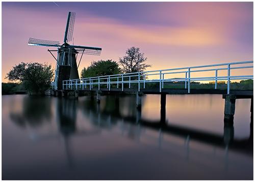
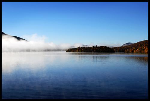
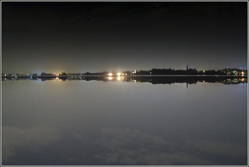
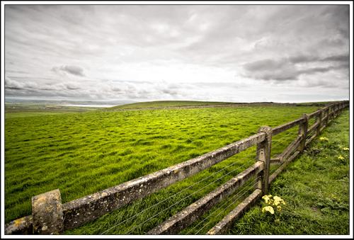
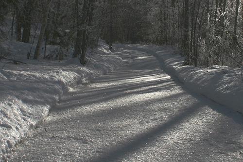
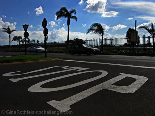
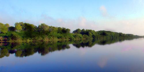
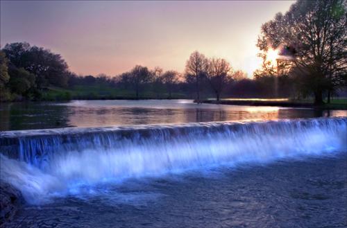
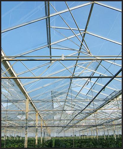
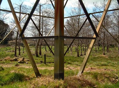
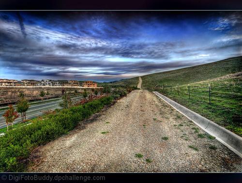
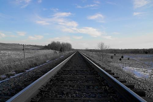
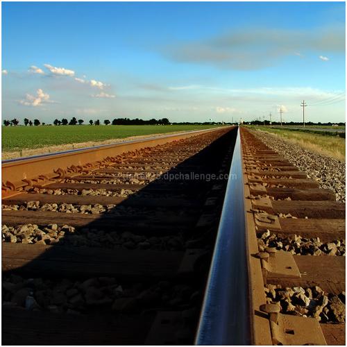
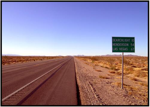
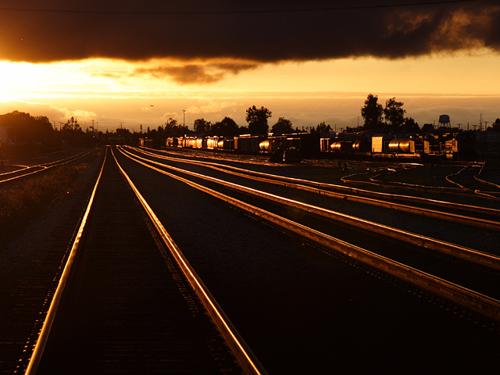
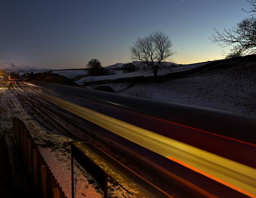
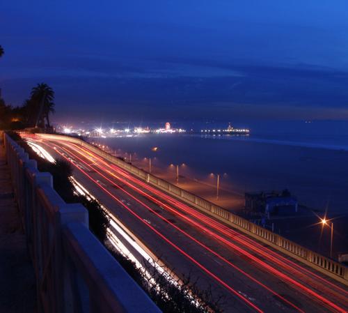
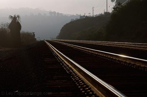
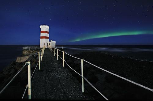
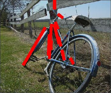
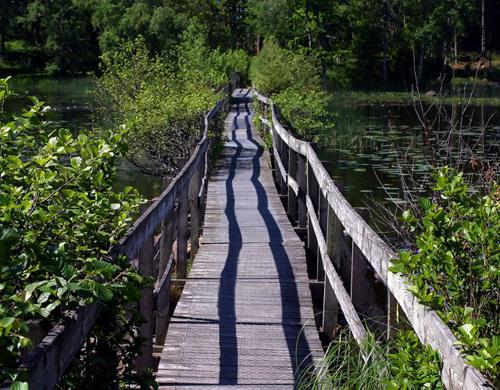
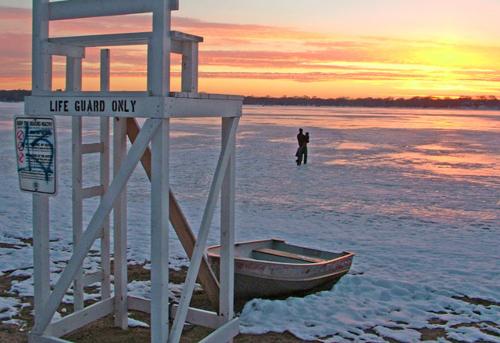
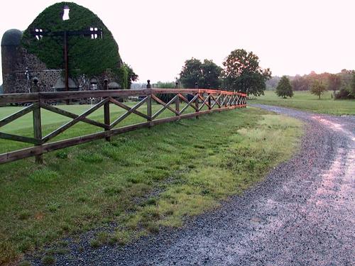
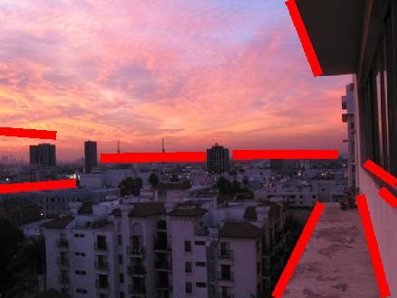
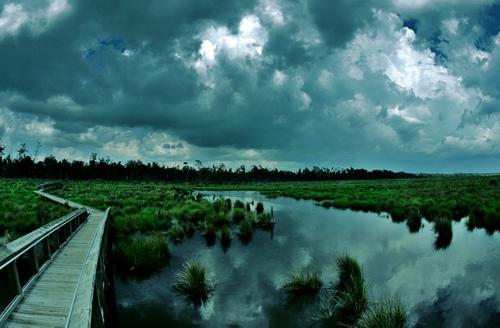
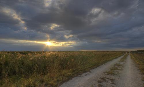
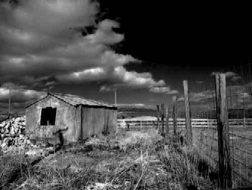
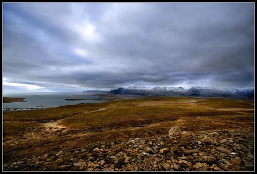
Figure 13: Example viewpoint-specific image retrieval results. Each row shows a query image (first image from the left) and the top-ranked images retrieved by our method. Last two rows show some failure cases.

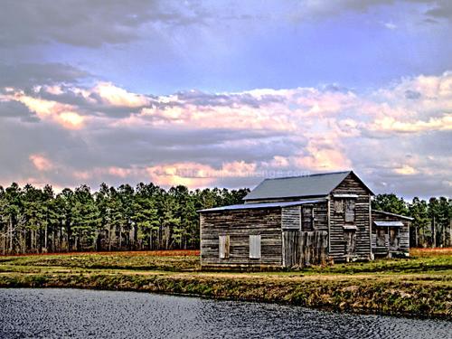
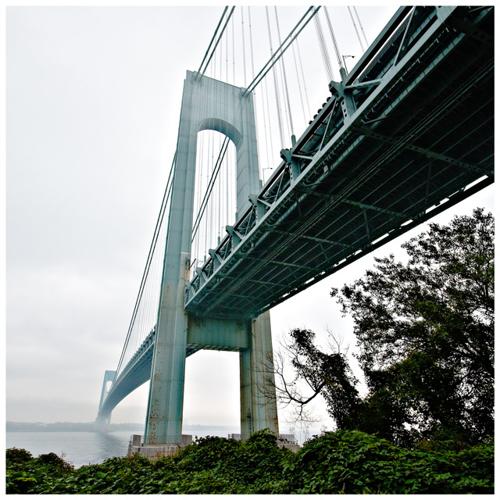
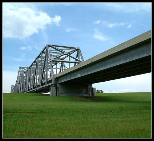
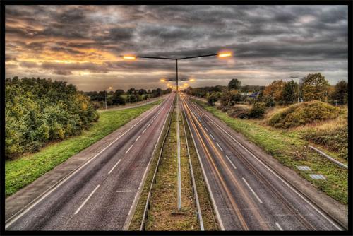
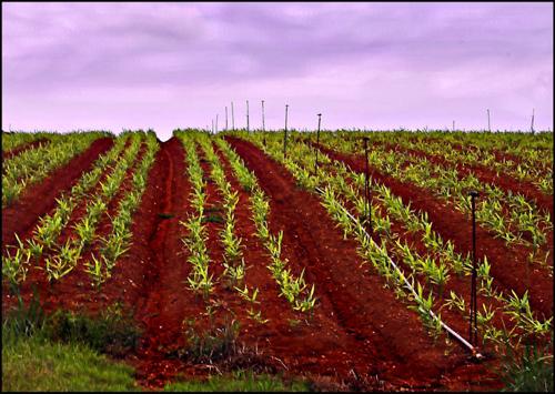
Figure 14: Comparison to state-of-the-art retrieval methods. For a query image, we show the top four or five images retrieved by different methods, where each row corresponds to one method. First row: Our method. Second row: CNN. Third row: HOG.

VI-B Case Studies

In our experiments, we use the entire “landscape” category of the AVA dataset to study the effectiveness of our new similarity measure. We first run our contour-based VP detection algorithm to detect the dominant VP in the 21,982 images in that category. We only keep those VPs with strength scores higher than 150 for this study because, as mentioned earlier (Section V-B), detections with low strength scores are often unreliable. If no dominant VP is detected in an image, we simply set the perspective similarity $D_{p}(I_{i},I_{j})=0$.

Figure 13 shows the top-ranked images for various query images in the AVA dataset. It is clear that our method is able to retrieve images with similar content and similar viewpoints as the query image. More importantly, the retrieved images exhibit a wide variety in terms of the photographic techniques used, including color, lighting, photographic elements, design principles, etc. Thus, by examining the exemplar images retrieved by our system, amateur photographers may conveniently learn useful techniques to improve the quality of their work. Below we examine a few cases:

1^st row, red boxes: This pair of photos highlight the importance of lighting in photography. Instead of taking the picture with an overcast sky, it is better to take the shot close to sunset with a clear sky, as the interplay of sunlight and shadows could make the photo more attractive. Also, it can be desirable to leave more water in the scene to better reflect such interplay.

6^th row, blue boxes: These three photos illustrate the different choices of framing and photo composition. While the query image uses a diagonal composition, alternative ways to shoot the bridge scene include using a vertical frame or lowering the camera to include the river.

9^th row, green boxes: This case shows an example where photographers sometimes choose unconventional aspect ratios (e.g., a wide view) to make the photo more interesting.

11^th row, yellow boxes: Compared to the query image, the retrieved image contains more vivid colors (the grass) and texture (the cloud).

The last two rows of Figure 13 show the typically failure cases of our method, in which we also plot the edges corresponding to the detected VP in the query image. In the first example, our VP detection method fails to detect the true dominant VP in the image. For the second example, while the detection is successful, our retrieval system is unable to find images with similar viewpoints. In real-world applications, however, we expect the size of the image database to be much larger than our experimental database (with $\sim$20K images), and the algorithm should be able to retrieve valid results.

VI-C Comparison to the State-of-the-Art

We compare our method to two popular retrieval systems, which are based on the HOG features [65, 66] and the CNN features, respectively. While many image retrieval methods exist in the literature, we choose these two because (i) the CNN features have been recently shown to achieve state-of-the-art performance on semantic image retrieval and (ii) similar to our method, the HOG features are known to be sensitive to image edges, thus providing a good baseline for comparison.

For HOG, We represent each image with a rigid grid-like HOG feature $\mathbf{x}_{i}$ [65, 66]. As suggested in [57], we limit its dimensionality to roughly $5K$ by resizing the images to $150\times 100$ or $100\times 150$ and using a cell size of 8 pixels. The feature vectors are normalized by subtracting the mean: $\mathbf{x}_{i}=\mathbf{x}_{i}-mean(\mathbf{x}_{i})$. We use the cosine distance as the similarity measure. For CNN, we directly use $D_{s}(I_{j},I_{j})$ discussed in Section VI-A as the final matching score. Obviously, our method reduces to CNN if we set $\gamma_{1}=\gamma_{2}=0$ in Eq. (12).

Figure 14 shows the best matches retrieved by all systems for various query images. Both CNN and our method are able to retrieve semantically relevant images. However, the images retrieved by CNN vary significantly in terms of the viewpoint. In contrast, out method retrieves images with similar viewpoints. While HOG is somewhat sensitive to the edge orientations (see the first and fourth examples in Figure 14), our method more effectively captures the viewpoints and perspective effects.

Quantitative human subject evaluation. We further perform a quantitative evaluation on the performance of our retrieval method. Unlike traditional image retrieval benchmarks, currently there is no dataset with ground truth composition (i.e., viewpoint) labels available. In view of this barrier, we instead conducted a user study which asked participants to manually compare the performance of our method with that of CNN based on their ability to retrieve images that have similar semantics and similar viewpoints. Note that we have excluded HOG from this study because (i) it performs substantially worse than our method and CNN, and (ii) we are particularly interested in the effectiveness of the new perspective similarity measure $D_{p}$.

In this study, a collection of 200 query images (with VP strength scores higher than 150) are randomly selected from our new dataset of 1,316 images that each containing a dominant VP (Section III). At our user study website, each participant is assigned with a subset of 30 randomly selected query images. For each query, we show the top-8 images retrieved by both systems and ask the participant to rank the performance of the two systems. To avoid any biases, no information about the two systems was provided during the study. Further, we randomly shuffled the order in which the results of the two systems are shown on each page.

We recruited 10 participants to this study, mostly graduate students with some basic photography knowledge. Overall, participants ranked our system better 76.7% of the time, whereas CNN received higher rankings only 23.3% of the time. This outcome suggests our system significantly outperforms the state-of-the-art for the viewpoint-specific image retrieval task.

VII Conclusions and Discussions

In this paper, we study an intriguing problem of detecting the dominant VP in natural landscape images. We develop a new VP detection method, which combines a contour-based edge detector with J-Linkage, and show that it outperforms state-of-the-art methods on a new ground truth dataset. The detected VPs and the associated image elements provides valuable information about the photo composition. As an application of our method, we develop a novel viewpoint-specific image retrieval system which can potentially provide useful on-site feedback to photographers.

VII-A Performance on Architecture Photos

While the primary focus of this paper is on natural scenes, we applied the proposed methods to images of structured man-made environments, e.g., architecture photos. For a dominant VP in an architecture photo, a large number of strong edges often converge to it. How does the performance of our dominant VP detection and selection methods compare to the state-of-the-art in such scenarios? Given that there are often more than one VP in architecture photos, would our image retrieval method perform as successfully under such complexity?

AVA architecture dataset. To study the performance of our methods on architecture photos, we again resort to the AVA dataset and use the 12,026 images under the category “architecture”. Following the same annotation procedure as described in Section III, for each image, we determine whether it contains a dominant VP and, if so, label its location. For consistency, we still restrict ourselves to the detection of a single dominant VP and do not consider images with two or more VPs carrying similar visual importance. As a result, we collected a total of 2,401 images with ground-truth annotations.

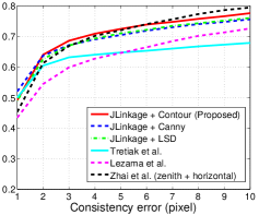
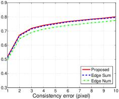
(a)	(b)

Figure 15: Experiments on architecture photos. (a) Dominant VP detection. (b) Dominant VP selection.

Dominant VP detection and selection experiment. Using the same experiment protocol and parameter settings as described in Section IV-C, we compare our contour-based VP detection method to the state-of-the-art. As one can see in Figure 15(a), our method achieves competitive performance on the architecture photos. Recall that our experiment setting actually favors Zhai et al. [36] in that we consider both the zenith VP and top-ranked horizontal VP detected by [36] in the evaluation. We also note that, in comparison to Figure 6, the gaps in performance among the three edge detection methods appear to be smaller on architecture photos. This finding actually highlights the importance of exploring global structures in natural scenes in which strong edges are often absent.

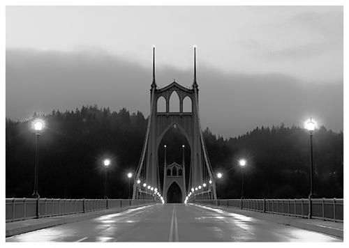
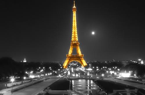
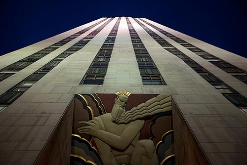
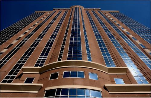
Figure 16: Comparison to state-of-the-art retrieval methods on architecture photos. For a query image, we show the top four or five images retrieved by different methods, where each row corresponds to one method. First row: Our method. Second row: CNN. Third row: HOG.

We have also explored the effectiveness of the strength measure proposed in Section V on architecture photos. As shown in Figure 15(b), our proposed measure and Edge Sum achieve very similar performance in selecting the dominant VP, and both outperform Edge Num. The result suggests that while considering edge length increases the accuracy, the impact of the distance from edge to the VP appears to be insignificant. This observation may be because, when there is a large number of edges, the length of the converging edges dominates the VP selection.

Viewpoint-specific image retrieval experiment. For this experiment, we use the entire “architecture” category of the AVA dataset. Using the same experiment protocol and parameter settings as in Section VI, we compare our method to HOG and CNN. Figure 16 shows the retrieval results for various query images in the AVA dataset.

To quantitatively evaluate the performance, we use the website developed in Section VI-C to conduct a user study on the retrieval results for architecture photos. We have again recruited 10 participants, mostly graduate students with some basic photography knowledge. Overall, our system is ranked better 70.0% of the time (compared to 76.7% for landscape images). We attribute the decrease in performance to the presence of multiple vanishing points in some architecture photos. As these VPs may carry similar visual weights, our method is limited to choosing one from all the candidates, which results in some ambiguity in the retrieval results. We show such a case in Figure 17 (first row), where our algorithm is able to detect the vertical VP in the images, but the horizontal orientation of the buildings remains ambiguous. Another type of failure cases results from issues with scene semantics, as shown in Figure 17 (second row). In this case, the CNN descriptor fails to capture the building in the query image, making the retrieved images less informative.

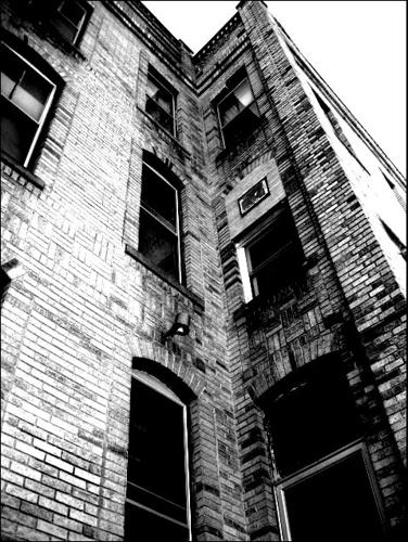
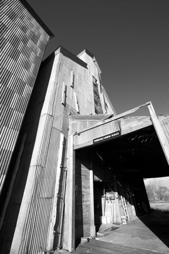
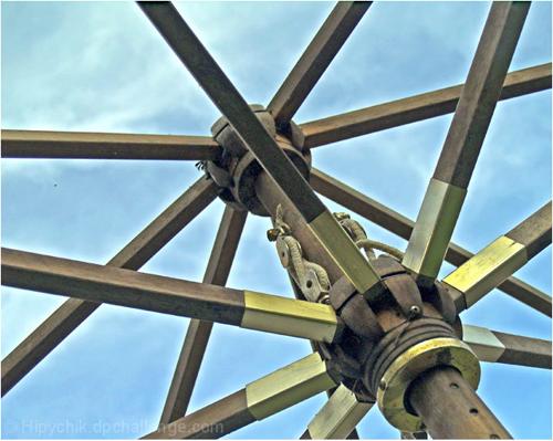
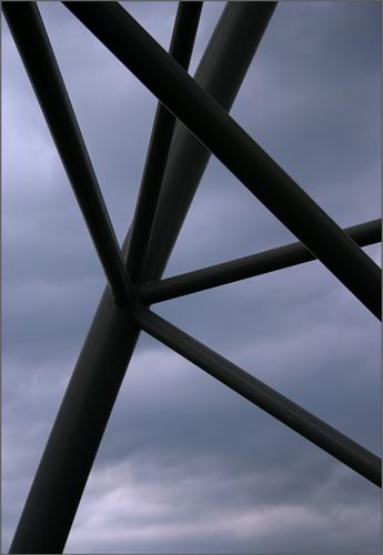
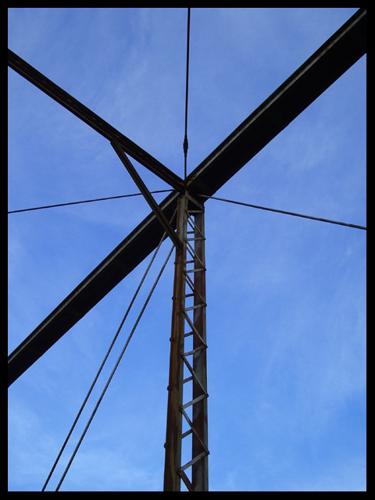
Figure 17: Some failure cases of our method on architecture photos. Each row shows a query image (first image from the left) and the top-ranked images retrieved by our method.

In summary, the experiment results on architecture photos demonstrate that the techniques we introduce in this paper are applicable to other scene types, and importantly, they are particularly suitable and effective for natural scenes.

VII-B Detecting Multiple Vanishing Points in Natural Scenes

So far we have restricted our attention to the dominant VP in the image. As another interesting extension, we examine how our method performs on natural landscape images when the number of VPs in each image is not fixed. We use the entire AVA landscape dataset and label all the VPs in each image. Note that a VP is labeled as long as there are two lines in the scene converging to it, and we no longer require the VPs to lie within or near the image frame. In this way, we have obtained 1,928 images with one or more VPs.

For fair comparison, in this experiment we keep the top-3 detections of each method, since three is the maximum number of VPs we have found in any image in the AVA landscape dataset. Note that for [36] we consider both the zenith VP and the top-3 horizontal VPs in the evaluation. For each ground truth VP in an image, we find the closest detection and compute the consistency error as given in Eq. (6). As one can see in Figure 18, the proposed method again outperforms all other methods. This result suggests that our method is not limited to the dominant VP, but that it can be employed as a general tool for VP detection in natural scenes.

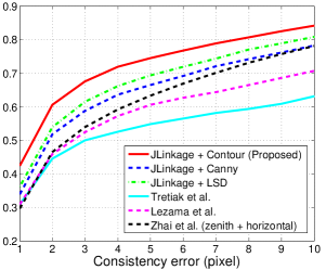
Figure 18: Experiment results on detecting multiple VPs in natural landscape images.

VII-C Limitations

One limitation of our current system is that it is not designed to handle images in which the linear perspective is absent. For example, to convey a sense of depth, other techniques such as diminishing objects and atmospheric perspective have also been used. Instead of relying solely on the linear perspective, experienced photographers often employ multiple design principles such as balance, contrast, unity, and illumination. In the future, we plan to explore these factors for extensive understanding of photo composition.

Zihan Zhou received the bachelor’s degree in Automation from Tsinghua University, Beijing, China, in 2007, and the MS and PhD degrees in Electrical and Computer Engineering from University of Illinois at Urbana-Champaign in 2010 and 2013, respectively. He is currently a faculty member in the College of Information Sciences and Technology at Pennsylvania State University. His research interests lie in computer vision and image processing, specially in developing new computational tools for efficient and robust discovery of low-dimensional data structure for 3D scene analysis and modeling. He is a member of the IEEE.

Farshid Farhat is a PhD candidate at the School of Electrical Engineering and Computer Science, The Pennsylvania State University. He obtained his B.Sc., M.Sc., and Ph.D. degrees in Electrical Engineering from Sharif University of Technology, Tehran, Iran. His current research interests include computer vision, image processing, distributed systems, and networking. He is working on the modeling and analysis of image composition and aesthetics using deep learning and image retrieval on different platforms ranging from smartphones to high-performance computing clusters.

James Z. Wang is a Professor of Information Sciences and Technology at The Pennsylvania State University. He received the bachelor’s degree in mathematics and computer science summa cum laude from the University of Minnesota, and the MS degree in mathematics, the MS degree in computer science and the PhD degree in medical information sciences, all from Stanford University. His research interests include computational aesthetics and emotions, automatic image tagging, image retrieval, and computerized analysis of paintings. He was a visiting professor at the Robotics Institute at Carnegie Mellon University (2007-2008), a lead special section guest editor of the IEEE Transactions on Pattern Analysis and Machine Intelligence (2008), and a program manager at the Office of the Director of the National Science Foundation (2011-2012). He was a recipient of a National Science Foundation Career award (2004).

References

- [1] B. P. Krages, Photography: The Art of Composition. Allworth Press, 2005.
- [2] S. Bhattacharya, R. Sukthankar, and M. Shah, “A framework for photo-quality assessment and enhancement based on visual aesthetics,” in Proc. ACM Multimedia Conf., 2010, pp. 271–280.
- [3] L. Liu, R. Chen, L. Wolf, and D. Cohen-Or, “Optimizing photo composition,” Comput. Graph. Forum, vol. 29, no. 2, pp. 469–478, 2010.
- [4] L. Yao, P. Suryanarayan, M. Qiao, J. Z. Wang, and J. Li, “Oscar: On-site composition and aesthetics feedback through exemplars for photographers,” International Journal of Computer Vision, vol. 96, no. 3, pp. 353–383, 2012.
- [5] B. Ni, M. Xu, B. Cheng, M. Wang, S. Yan, and Q. Tian, “Learning to photograph: A compositional perspective,” IEEE Trans. on Multimedia, vol. 15, no. 5, pp. 1138–1151, 2013.
- [6] R. Hartley and A. Zisserman, Multiple View Geometry in Computer Vision. Cambridge: Cambridge University Press, 2000.
- [7] J.-P. Tardif, “Non-iterative approach for fast and accurate vanishing point detection,” in Proc. Int. Conf. on Computer Vision, 2009, pp. 1250–1257.
- [8] E. Tretiak, O. Barinova, P. Kohli, and V. S. Lempitsky, “Geometric image parsing in man-made environments,” International Journal of Computer Vision, vol. 97, no. 3, pp. 305–321, 2012.
- [9] H. Wildenauer and A. Hanbury, “Robust camera self-calibration from monocular images of manhattan worlds,” in Proc. IEEE Conf. Comput. Vis. Pattern Recog., 2012, pp. 2831–2838.
- [10] Y. Xu, S. Oh, and A. Hoogs, “A minimum error vanishing point detection approach for uncalibrated monocular images of man-made environments,” in Proc. IEEE Conf. Comput. Vis. Pattern Recog., 2013, pp. 1376–1383.
- [11] J. Lezama, R. G. von Gioi, G. Randall, and J. Morel, “Finding vanishing points via point alignments in image primal and dual domains,” in Proc. IEEE Conf. Comput. Vis. Pattern Recog., 2014, pp. 509–515.
- [12] D. A. Lauer and S. Pentak, Design Basics. Cengage Learning, 2011.
- [13] J. Canny, “A computational approach to edge detection,” IEEE Trans. Pattern Anal. Mach. Intell., vol. 8, no. 6, pp. 679–698, 1986.
- [14] R. G. von Gioi, J. Jakubowicz, J. Morel, and G. Randall, “LSD: A fast line segment detector with a false detection control,” IEEE Trans. Pattern Anal. Mach. Intell., vol. 32, no. 4, pp. 722–732, 2010.
- [15] R. Toldo and A. Fusiello, “Robust multiple structures estimation with j-linkage,” in Proc. European Conf. on Computer Vision (1), 2008, pp. 537–547.
- [16] B. Caprile and V. Torre, “Using vanishing points for camera calibration,” International Journal of Computer Vision, vol. 4, no. 2, pp. 127–139, 1990.
- [17] R. Cipolla, T. Drummond, and D. P. Robertson, “Camera calibration from vanishing points in image of architectural scenes,” in Proc. British Machine Vision Conf., 1999, pp. 1–10.
- [18] M. E. Antone and S. J. Teller, “Automatic recovery of relative camera rotations for urban scenes,” in Proc. IEEE Conf. Comput. Vis. Pattern Recog., 2000, pp. 2282–2289.
- [19] J. Kosecká and W. Zhang, “Video compass,” in Proc. European Conf. on Computer Vision (4), 2002, pp. 476–490.
- [20] P. Denis, J. H. Elder, and F. J. Estrada, “Efficient edge-based methods for estimating manhattan frames in urban imagery,” in Proc. European Conf. on Computer Vision, 2008, pp. 197–210.
- [21] F. A. Andaló, G. Taubin, and S. Goldenstein, “Efficient height measurements in single images based on the detection of vanishing points,” Computer Vision and Image Understanding, vol. 138, pp. 51–60, 2015.
- [22] D. Hoiem, A. A. Efros, and M. Hebert, “Putting objects in perspective,” International Journal of Computer Vision, vol. 80, no. 1, pp. 3–15, 2008.
- [23] P. Parodi and G. Piccioli, “3d shape reconstruction by using vanishing points,” IEEE Trans. Pattern Anal. Mach. Intell., vol. 18, no. 2, pp. 211–217, 1996.
- [24] A. Criminisi, I. D. Reid, and A. Zisserman, “Single view metrology,” International Journal of Computer Vision, vol. 40, no. 2, pp. 123–148, 2000.
- [25] S. T. Barnard, “Interpreting perspective image,” Artif. Intell., vol. 21, no. 4, pp. 435–462, 1983.
- [26] L. Quan and R. Mohr, “Determining perspective structures using hierarchical hough transform,” Pattern Recognition Letters, vol. 9, no. 4, pp. 279–286, 1989.
- [27] R. T. Collins and R. S. Weiss, “Vanishing point calculation as a statistical inference on the unit sphere,” in Proc. Int. Conf. on Computer Vision, 1990, pp. 400–403.
- [28] B. Brillault-O’Mahony, “New method for vanishing point detection,” CVGIP: Image Understanding, vol. 54, no. 2, pp. 289–300, 1991.
- [29] T. Tuytelaars, M. Proesmans, and L. J. V. Gool, “The cascaded hough transforms,” in ICIP (2), 1997, pp. 736–739.
- [30] J. A. Shufelt, “Performance evaluation and analysis of vanishing point detection techniques,” IEEE Trans. Pattern Anal. Mach. Intell., vol. 21, no. 3, pp. 282–288, 1999.
- [31] C. Rother, “A new approach for vanishing point detection in architectural environments,” in Proc. British Machine Vision Conf., 2000, pp. 1–10.
- [32] A. Almansa, A. Desolneux, and S. Vamech, “Vanishing point detection without any A priori information,” IEEE Trans. Pattern Anal. Mach. Intell., vol. 25, no. 4, pp. 502–507, 2003.
- [33] G. Schindler and F. Dellaert, “Atlanta world: An expectation maximization framework for simultaneous low-level edge grouping and camera calibration in complex man-made environments,” in Proc. IEEE Conf. Comput. Vis. Pattern Recog. (1), 2004, pp. 203–209.
- [34] G. F. McLean and D. Kotturi, “Vanishing point detection by line clustering,” IEEE Trans. Pattern Anal. Mach. Intell., vol. 17, no. 11, pp. 1090–1095, 1995.
- [35] A. Vedaldi and A. Zisserman, “Self-similar sketch,” in Proc. European Conf. on Computer Vision, 2012, pp. 87–100.
- [36] M. Zhai, S. Workman, and N. Jacobs, “Detecting vanishing points using global image context in a non-manhattan world,” in Proc. IEEE Conf. Comput. Vis. Pattern Recog., 2016, pp. 5657–5665.
- [37] J. M. Coughlan and A. L. Yuille, “Manhattan world: Orientation and outlier detection by bayesian inference,” Neural Computation, vol. 15, no. 5, pp. 1063–1088, 2003.
- [38] F. M. Mirzaei and S. I. Roumeliotis, “Optimal estimation of vanishing points in a manhattan world,” in Proc. Int. Conf. on Computer Vision, 2011, pp. 2454–2461.
- [39] J. C. Bazin, Y. Seo, C. Demonceaux, P. Vasseur, K. Ikeuchi, I. Kweon, and M. Pollefeys, “Globally optimal line clustering and vanishing point estimation in manhattan world,” in Proc. IEEE Conf. Comput. Vis. Pattern Recog., 2012, pp. 638–645.
- [40] M. Antunes and J. P. Barreto, “A global approach for the detection of vanishing points and mutually orthogonal vanishing directions,” in Proc. IEEE Conf. Comput. Vis. Pattern Recog., 2013, pp. 1336–1343.
- [41] C. Rasmussen, “Grouping dominant orientations for ill-structured road following,” in Proc. IEEE Conf. Comput. Vis. Pattern Recog. (1), 2004, pp. 470–477.
- [42] H. Kong, J.-Y. Audibert, and J. Ponce, “Vanishing point detection for road detection,” in Proc. IEEE Conf. Comput. Vis. Pattern Recog., 2009, pp. 96–103.
- [43] P. Moghadam, J. A. Starzyk, and W. S. Wijesoma, “Fast vanishing-point detection in unstructured environments,” IEEE Trans. on Image Processing, vol. 21, no. 1, pp. 425–430, 2012.
- [44] F. Zhang, M. Wang, and S. Hu, “Aesthetic image enhancement by dependence-aware object recomposition,” IEEE Trans. Multimedia, vol. 15, no. 7, pp. 1480–1490, 2013.
- [45] C. Fang, Z. Lin, R. Mech, and X. Shen, “Automatic image cropping using visual composition, boundary simplicity and content preservation models,” in Proc. ACM Multimedia Conf., 2014, pp. 1105–1108.
- [46] M. B. Islam, W. Lai-Kuan, and W. Chee-Onn, “A survey of aesthetics-driven image recomposition,” Multimedia Tools and Applications, pp. 1–26, 2016.
- [47] J. Yan, S. Lin, S. B. Kang, and X. Tang, “Change-based image cropping with exclusion and compositional features,” International Journal of Computer Vision, vol. 114, no. 1, pp. 74–87, 2015.
- [48] R. Hong, L. Zhang, and D. Tao, “Unified photo enhancement by discovering aesthetic communities from flickr,” IEEE Trans. Image Processing, vol. 25, no. 3, pp. 1124–1135, 2016.
- [49] H. Su, T. Chen, C. Kao, W. H. Hsu, and S. Chien, “Preference-aware view recommendation system for scenic photos based on bag-of-aesthetics-preserving features,” IEEE Trans. on Multimedia, vol. 14, no. 3-2, pp. 833–843, 2012.
- [50] S. Ma, Y. Fan, and C. W. Chen, “Pose maker: A pose recommendation system for person in the landscape photographing,” in Proc. ACM Multimedia Conf., 2014, pp. 1053–1056.
- [51] P. Xu, H. Yao, R. Ji, X. Liu, and X. Sun, “Where should I stand? learning based human position recommendation for mobile photographing,” Multimedia Tools and Applications, vol. 69, no. 1, pp. 3–29, 2014.
- [52] Y. S. Rawat and M. S. Kankanhalli, “Context-aware photography learning for smart mobile devices,” ACM Trans. on Multimedia Computing, Communications, and Applications, vol. 12, no. 1s, p. 19, 2015.
- [53] W. Yin, T. Mei, C. W. Chen, and S. Li, “Socialized mobile photography: Learning to photograph with social context via mobile devices,” IEEE Trans. Multimedia, vol. 16, no. 1, pp. 184–200, 2014.
- [54] A. W. Smeulders, M. Worring, S. Santini, A. Gupta, and R. Jain, “Content-based image retrieval at the end of the early years,” IEEE Trans. Pattern Anal. Mach. Intell., vol. 22, no. 12, pp. 1349–1380, 2000.
- [55] R. Datta, D. Joshi, J. Li, and J. Z. Wang, “Image retrieval: Ideas, influences, and trends of the new age,” ACM Computing Surveys, vol. 40, no. 2, pp. 5:1–60, 2008.
- [56] H. Jegou, M. Douze, C. Schmid, and P. Pérez, “Aggregating local descriptors into a compact image representation,” in Proc. IEEE Conf. Comput. Vis. Pattern Recog., 2010, pp. 3304–3311.
- [57] A. Shrivastava, T. Malisiewicz, A. Gupta, and A. A. Efros, “Data-driven visual similarity for cross-domain image matching,” ACM Trans. on Graphics, vol. 30, no. 6, p. 154, 2011.
- [58] A. S. Razavian, H. Azizpour, J. Sullivan, and S. Carlsson, “CNN features off-the-shelf: An astounding baseline for recognition,” in Proc. IEEE Conf. Comput. Vis. Pattern Recog. Workshops, 2014, pp. 512–519.
- [59] Z. Zhou, S. He, J. Li, and J. Z. Wang, “Modeling perspective effects in photographic composition,” in Proc. ACM Multimedia Conf., 2015, pp. 301–310.
- [60] N. Murray, L. Marchesotti, and F. Perronnin, “AVA: A large-scale database for aesthetic visual analysis,” in Proc. IEEE Conf. Comput. Vis. Pattern Recog., 2012, pp. 2408–2415.
- [61] P. Arbelaez, M. Maire, C. Fowlkes, and J. Malik, “Contour detection and hierarchical image segmentation,” IEEE Trans. Pattern Anal. Mach. Intell., vol. 33, no. 5, pp. 898–916, 2011.
- [62] D. R. Martin, C. C. Fowlkes, and J. Malik, “Learning to detect natural image boundaries using local brightness, color, and texture cues,” IEEE Trans. Pattern Anal. Mach. Intell., vol. 26, no. 5, pp. 530–549, 2004.
- [63] K. Chatfield, K. Simonyan, A. Vedaldi, and A. Zisserman, “Return of the devil in the details: Delving deep into convolutional nets,” in Proc. British Machine Vision Conf., 2014.
- [64] S. Lazebnik, C. Schmid, and J. Ponce, “Beyond bags of features: Spatial pyramid matching for recognizing natural scene categories,” in Proc. IEEE Conf. Comput. Vis. Pattern Recog., 2006, pp. 2169–2178.
- [65] N. Dalal and B. Triggs, “Histograms of oriented gradients for human detection,” in Proc. IEEE Conf. Comput. Vis. Pattern Recog., 2005, pp. 886–893.
- [66] P. F. Felzenszwalb, R. B. Girshick, D. A. McAllester, and D. Ramanan, “Object detection with discriminatively trained part-based models,” IEEE Trans. Pattern Anal. Mach. Intell., vol. 32, no. 9, pp. 1627–1645, 2010.