The Bayesian Low-Rank Determinantal Point Process Mixture Model

Abstract

Determinantal point processes (DPPs) are an elegant model for encoding probabilities over subsets, such as shopping baskets, of a ground set, such as an item catalog. They are useful for a number of machine learning tasks, including product recommendation. DPPs are parametrized by a positive semi-definite kernel matrix. Recent work has shown that using a low-rank factorization of this kernel provides remarkable scalability improvements that open the door to training on large-scale datasets and computing online recommendations, both of which are infeasible with standard DPP models that use a full-rank kernel. In this paper we present a low-rank DPP mixture model that allows us to represent the latent structure present in observed subsets as a mixture of a number of component low-rank DPPs, where each component DPP is responsible for representing a portion of the observed data. The mixture model allows us to effectively address the capacity constraints of the low-rank DPP model. We present an efficient and scalable Markov Chain Monte Carlo (MCMC) learning algorithm for our model that uses Gibbs sampling and stochastic gradient Hamiltonian Monte Carlo (SGHMC). Using an evaluation on several real-world product recommendation datasets, we show that our low-rank DPP mixture model provides substantially better predictive performance than is possible with a single low-rank or full-rank DPP, and significantly better performance than several other competing recommendation methods in many cases.

1 Introduction

Online shopping activity has grown rapidly in recent years. Central to the online retail experience is the recommendation task of “basket completion”, where we seek to compute predictions for the next item that should be added to a shopping basket, given a set of items already present in the basket. Determinantal point processes (DPPs) offer an attractive model for basket completion, since they jointly model set diversity and item quality or popularity. DPPs also offer a compact parameterization and efficient algorithms for performing inference.

A distribution over sets that models diversity is of particular interest when recommendations are complementary. For example, consider a shopping basket that contains a smartphone and a SIM card. A collaborative filtering method based on user and item similarities, such as a matrix factorization model [26], would tend to provide recommendations that are similar to the items already present in the basket but not necessarily complementary. In this example, matrix factorization might recommend other similar smartphones to complete this basket, which may not be appropriate since the basket already contains a smartphone. In contrast, a complementary recommendation for this basket might be a smartphone case, rather than another smartphone. In this setting, DPPs would be used to learn the inherent item diversity present within the observed sets (baskets) that users purchase, and hence can provide such complementary recommendations.

DPPs have been used for a variety of machine learning tasks [15, 17, 18]. DPPs can be parameterized by a $M\times M$ positive semi-definite $\mathbf{L}$ matrix, where $M$ is the size of the item catalog. There has been some work focused on learning DPPs from observed data consisting of example subsets [1, 8, 9, 11, 16, 22], which is a challenging learning task that is conjectured to be NP-hard [17]. Some of this recent work has involved learning a nonparametric full-rank $\mathbf{L}$ matrix [11, 22] that does not constrain $\mathbf{L}$ to take a particular parametric form, while other recent work has involved learning a low-rank factorization of this nonparametric $\mathbf{L}$ matrix [8, 9]. A low-rank factorization of $\mathbf{L}$ enables substantial improvements in runtime performance compared to a full-rank DPP model during training and when computing predictions, on the order of 10-20x or more, with predictive performance that is equivalent to or better than a full-rank model.

While the low-rank DPP model scales well, it has a fundamental limitation regarding model capacity due to the nature of the low-rank factorization of $\mathbf{L}$. The low-rank DPP mixture model allows us to address these capacity constraints. As we explain in Section 2.1, a $K$-rank factorization of $\mathbf{L}$ has an implicit constraint on the space of possible subsets, since it places zero probability mass on subsets (baskets) with more than $K$ items. When trained on a dataset containing baskets with at most $K$ items, we observe from the results in  [8] that this constraint is reasonable and that the rank-$K$ DPP provides predictive performance that is approximately equivalent to that of the full-rank DPP trained on the same dataset. Therefore, in this scenario the rank-$K$ DPP can be seen as a good approximation of the full-rank DPP. However, we empirically observe that the rank-$K$ DPP generally does not provide improved predictive performance for values of $K$ greater than the size of the largest basket in the data. Thus, for a dataset containing baskets no larger than size $K$, there is generally no utility in increasing the number of low-rank DPP item trait dimensions beyond $K$, which establishes an upper bound on the capacity of the model. This limitation motivates us to find a way to move beyond the capacity of the low-rank DPP model. We present a mixture model composed of a number of component low-rank DPPs as an effective method for addressing the capacity constraints of the low-rank DPP. In the low-rank DPP mixture model, each component low-rank DPP is responsible for modeling only a subset of the baskets in the full dataset. In the case of the conventional low-rank DPP model, the low-rank DPP is responsible for modeling the entire dataset. Therefore, the mixture model provides us with capacity beyond that available with only a single low-rank DPP.

Our work makes the following contributions:

1. We present a Bayesian low-rank DPP mixture model, which represents the latent structure present in observed subsets as a mixture of a number of component low-rank DPPs. The mixture model allows us to effectively address the capacity constraints of the low-rank DPP model.

2. We present an efficient and parallelizable learning algorithm for our model that utilizes Gibbs sampling and stochastic gradient Hamiltonian Monte Carlo (SGHMC).

3. A detailed experimental evaluation on several real-world datasets shows that our mixture model provides significantly better predictive performance than existing DPP models. Our model also provides significantly better predictive performance than several other state-of-the-art recommendation methods in many cases.

2 Model

DPPs originated in statistical mechanics [21], where they were used to model distributions of fermions. Fermions are particles that obey the Pauli exclusion principle, which indicates that no two fermions can occupy the same quantum state. As a result, systems of fermions exhibit a repulsion or “anti-bunching” effect, which is described by a DPP. This repulsive behavior is a key characteristic of DPPs, which makes them a capable model for diversity. We now proceed with some details of DPPs, including how they are defined and a method for efficient learning.

2.1 Background

A point process is a distribution over configurations of points selected from a ground set $\mathcal{Y}$, which are finite subsets of $\mathcal{Y}$. In this paper we deal only with discrete DPPs, which describe a distribution over subsets of a discrete ground set of items $\mathcal{Y}={1,2,\ldots,M}$, which we also call the item catalog. A discrete DPP on $\mathcal{Y}$ is a probability measure $\mathcal{P}$ on $2^{\mathcal{Y}}$ (the power set or set of all subsets of $\mathcal{Y}$), such that for any $A\subseteq\mathcal{Y}$, the probability $\mathcal{P}(A)$ is specified by $\mathcal{P}(A)\propto\det(\mathbf{L}_{A})$. In the context of basket completion, $\mathcal{Y}$ is the item catalog (inventory of items on sale), and $A$ is the subset of items in a user’s basket; there are $2^{|\mathcal{Y}|}$ possible baskets. The notation $\mathbf{L}_{A}$ denotes the principal submatrix of the DPP kernel $\mathbf{L}$ indexed by the items in $A$, which is the restriction of $\mathbf{L}$ to the rows and columns indexed by the elements of $A$: $\mathbf{L}_{A}\equiv[\mathbf{L}_{ij}]_{i,j\in A}$. Intuitively, the diagonal entry $L_{ii}$ of the kernel matrix $\mathbf{L}$ captures the importance or quality of item $i$, while the off-diagonal entry $L_{ij}=L_{ji}$ measures the similarity between items $i$ and $j$.

The normalization constant for $\mathcal{P}$ follows from the observation that $\sum_{A^{\prime}\subseteq\mathcal{Y}}\det(\mathbf{L}_{A^{\prime}})=\det(\mathbf{L}+\mathbf{I})$. The value $\det(\mathbf{L}_{A})$ associates a “volume” to basket $A$ from a geometric viewpoint, and its probability is normalized by the volumes of all possible baskets $A^{\prime}\subseteq\mathcal{Y}$. Therefore, we have

$$\mathcal{P}(A)=\frac{\det(\mathbf{L}_{A})}{\det(\mathbf{L}+\mathbf{I})}\ .$$ (1)

We use a low-rank factorization of the $M\times M$ $\mathbf{L}$ matrix,

$$\mathbf{L}=\mathbf{V}\mathbf{V}^{T}\ ,$$ (2)

for the $M\times K$ matrix $\mathbf{V}$, where $M$ is the number of items in the item catalog and $K$ is the number of latent trait dimensions. This low-rank factorization of $\mathbf{L}$ leads to significant efficiency improvements compared to a model that uses a full-rank $\mathbf{L}$ matrix when it comes to model learning and computing predictions [8]. This also places an implicit constraint on the space of subsets of $\mathcal{Y}$, since the model is restricted to place zero probability mass on subsets with more than $K$ items (all eigenvalues of $\mathbf{L}$ beyond $K$ are zero). We see this from the observation that a sample from a DPP will not be larger than the rank of $\mathbf{L}$ [10].

2.2 Model Specification and Learning

Figure 1: A graphical model for the low-rank DPP model.

Figure 2: A graphical model for the low-rank DPP mixture model.

We begin by describing DPP learning and the Bayesian low-rank DPP model [9], since our DPP mixture model builds on these concepts. The DPP learning task is to fit a DPP kernel $\mathbf{L}$ based on a collection of $N$ observed subsets $\mathcal{A}=\{A_{1},\ldots,A_{N}\}$, where each subset $A_{n}$ is composed of items from the item catalog $\mathcal{Y}$. These observed subsets in $\mathcal{A}$ constitute our training data, and our task is to infer $\mathbf{L}$ from $\mathcal{A}$. The log-likelihood for seeing $\mathcal{A}$ is

$$f(\mathbf{V}) =\log\mathcal{P}(\mathcal{A}|\mathbf{V})=\sum_{n=1}^{N}\log\mathcal{P}(A_{n}|\mathbf{V})$$ (3)

$$=\sum_{n=1}^{N}\log\det(\mathbf{L}_{[n]})-N\log\det(\mathbf{L}+\mathbf{I})$$ (4)

where $[n]$ indexes the observed subsets in $\mathcal{A}$. Recall from (2) that $\mathbf{L}=\mathbf{V}\mathbf{V}^{T}$.

Figure 1 shows the graphical model for the Bayesian low-rank DPP model. We place a multivariate Gaussian prior on each item in our model. Our prior distribution on $\mathbf{V}$ is given by

$$p(\mathbf{V}|\gamma)=\prod_{i=1}^{M}\mathcal{N}(\mathbf{v}_{i};\mathbf{0},\gamma^{-1}\mathbf{I})$$ (5)

where $\mathbf{v}_{i}$ is the row vector from $\mathbf{V}$ for item $i$, and all items $i$ share the same precision $\gamma$. We furthermore place a conjugate gamma prior on $\gamma$: $p(\gamma|a_{0},b_{0})=\text{Gamma}(\gamma;a_{0},b_{0})$. The joint distribution over $\mathcal{A}$, $\mathbf{V}$ and $\gamma$, as depicted in Figure 1, is

$$p(\mathcal{A},\mathbf{V},\gamma|a_{0},b_{0}) =\mathcal{P}(\mathcal{A}|\mathbf{V})\,p(\mathbf{V}|\gamma)\,p(\gamma|a_{0},b_{0})\ .$$ (6)

For our Bayesian low-rank DPP mixture model, we consider a mixture model composed of $W$ component low-rank DPPs:

$$p(\mathcal{A}_{n}|\underline{\mathbf{V}},\boldsymbol{\phi})=\sum_{w=1}^{W}\phi_{w}\mathcal{P}(\mathcal{A}_{n}|\mathbf{V}_{w})$$ (7)

where $\underline{\mathbf{V}}$ denotes the collection of $\mathbf{V}_{w}$ components for all $W$, $\{\mathbf{V}_{w}\}_{w=1}^{W}$. This is a convex combination of the $W$ low-rank DPP components, where the mixing weights $\phi_{w}$ satisfy $0\leq\phi_{w}\leq 1$ and $\sum_{w=1}^{W}\phi_{w}=1$.

If we use the formulation of the Bayesian low-rank DPP model described above, then we have the following model specification for a low-rank DPP mixture model:

$$W =\text{number of mixture components}$$

$$N =\text{number of observed sets}$$

$$\mathcal{Y} =\text{item catalog}$$

$$M =\text{number of items in }\mathcal{Y}$$

$$K =\text{\parbox{170.71652pt}{number of item trait dimensions for the component low-rank DPPs}}$$

$$A_{n=1\ldots N} =\text{observation }n$$

$$\phi_{w=1\ldots W},\boldsymbol{\phi} =\text{\parbox{170.71652pt}{$W$-dimensional vector composed of all the individual $\phi_{w}$; must sum to 1}}$$

$$\mathbf{V}_{w=1\ldots W} =\text{\parbox{170.71652pt}{item trait matrix for low-rank DPP component $w$}}$$

$$\mathbf{z}_{n=1\ldots N} =\text{component of observation }n$$

$$a_{0},b_{0},\alpha =\text{shared hyperparameters}$$

$$\boldsymbol{\phi} \sim\text{Symmetric-Dirichlet}_{W}(\alpha)$$

$$\mathbf{z}_{n=1\ldots N} \sim\text{Categorical}(\boldsymbol{\phi})$$

$$\gamma_{w} \sim\text{Gamma}(\gamma_{w};a,b)$$

$$\mathbf{V}_{w} \sim\prod_{i=1}^{M}\mathcal{N}(\mathbf{v}_{wi}|0,\gamma_{w}^{-1}\mathbf{I})$$

$$A_{n=1\ldots N} \sim\mathcal{P}(\mathbf{V}_{z_{n}})$$ (8)

where $\mathbf{v}_{wi}$ is the row vector from $\mathbf{V}_{w}$ for mixture component $w$ and item $i$. We set $\alpha=\frac{1}{W}$. With this specification for the Dirichlet prior, for $W$ set to a conservative upper bound on the number of occupied mixture components, the model approximates a Dirichlet process mixture model [14], where redundant mixture components are automatically given zero weight during learning [28]. We find $W=100$ works well for the datasets we evaluated. Figure 2 shows the graphical model for our low-rank DPP mixture model. To draw samples from the posterior $p(\mathbf{V}_{w},\boldsymbol{\phi}|\mathcal{A},\alpha,\gamma_{w})$, for $w=1\ldots W$, we use the Gibbs sampling algorithm shown in Algorithm 1.

We can write $\mathbf{z}_{n}$ as a $W$-dimensional binary random variable having a 1-of-$W$ representation in which a particular element $z_{nw}$ is equal to 1 if the $n$th observation is drawn from the $w$th mixture component, and all other elements are equal to 0. $\mathbf{Z}$ is a $N\times W$ matrix, where $\mathbf{z}_{n}$ is a row vector from this matrix.

We can write the joint likelihood function for this model as

$$p(\mathcal{A},\mathbf{Z}|\underline{\mathbf{V}},\boldsymbol{\phi}) =\prod_{n=1}^{N}\prod_{w=1}^{W}\phi_{w}^{z_{nw}}\mathcal{P}(A_{n}|\mathbf{V}_{w})^{z_{nw}}\ .$$ (9)

The conditional distribution $p(\mathbf{Z}|\mathcal{A},\underline{\mathbf{V}},\boldsymbol{\phi})$ is

$$p(\mathbf{Z}|\mathcal{A},\underline{\mathbf{V}},\boldsymbol{\phi}) \propto\prod_{n=1}^{N}\prod_{w=1}^{W}\left(\phi_{w}\mathcal{P}(A_{n}|\mathbf{V}_{w})\right)^{z_{nw}}\ .$$ (10)

Therefore, we can draw samples for each discrete assignment $\mathbf{z}_{n}$ from

$$p(\mathbf{z}_{n}|A_{n},\underline{\mathbf{V}},\boldsymbol{\phi})\propto\exp\Bigg{\{}\sum_{w=1}^{W}z_{nw}\left(\log\phi_{w}+f(A_{n}|\mathbf{V}_{w})\right)\Bigg{\}}$$

directly, as each $p(\mathbf{z}_{n}|A_{n},\mathbf{V}_{w},\boldsymbol{\phi})$ is an independent categorical distribution. Note that $f(A_{n}|\mathbf{V}_{w})$ is the DPP log-likelihood (Equation 4) for a particular observation $A_{n}$. Subtract the maximum $m=\max_{w}(\log\phi_{w}+f(A_{n}|\mathbf{V}_{w}))$ everywhere,

$$p(z_{nw}=1|\mathcal{A},\underline{\mathbf{V}},\boldsymbol{\phi})=\frac{\exp\big{\{}\log\phi_{w}+f(A_{n}|\mathbf{V}_{w})-m\big{\}}}{\sum_{w^{\prime}=1}^{W}\exp\big{\{}\log\phi_{w^{\prime}}+f(A_{n}|\mathbf{V}_{w^{\prime}})-m\big{\}}}\ ,$$ (11)

so that the biggest exponentiated component is $\exp(0)$, and normalize to sum to one. Then draw the discrete index for which $z_{nw}=1$.

The conditional distribution $p(\boldsymbol{\phi}|\mathcal{A},\mathbf{Z},\alpha)$ is

$$p(\boldsymbol{\phi}|\mathcal{A},\mathbf{Z},\alpha) \propto\prod_{n=1}^{N}\text{Cat}(\mathbf{z}_{n}|\boldsymbol{\phi})\text{ Symmetric-Dirichlet}(\boldsymbol{\phi}|\alpha)$$

$$=\text{Dirichlet}\left(\boldsymbol{\phi}|\alpha+\sum_{n=1}^{N}z_{n1},\ldots,\alpha+\sum_{n=1}^{N}z_{nw}\right)$$ (12)

and is sampled in Line 6 in Algorithm 1.

The conditional distribution $p(\gamma_{w}|\mathbf{V}_{w},a_{0},b_{0})$ is

$$\gamma_{w}|\mathbf{V}_{w},a_{0},b_{0} \sim\text{Gamma}(\gamma_{w};a,b)$$

$$a =a_{0}+\frac{MK}{2}$$

$$b =b_{0}+\frac{1}{2}\sum_{i=1}^{M}\|\mathbf{v}_{wi}\|^{2}\ ,$$ (13)

and is sampled in Line 8 in Algorithm 1.

The conditional distribution $p(\mathbf{V}_{w}|\mathcal{A},\mathbf{Z},\gamma_{w})$ is

$$p(\mathbf{V}_{w}|\mathcal{A},\mathbf{Z},\gamma_{w}) \propto\prod_{n=1}^{N}\Bigg{(}\exp\big{(}f(A_{n}|\mathbf{V}_{w})\big{)}\Bigg{.}$$

$$\qquad\Bigg{.}{}\prod_{i=1}^{M}\mathcal{N}(\mathbf{v}_{wi}|\mathbf{0},\gamma_{w}^{-1}\mathbf{I})\Bigg{)}^{z_{nw}}$$

$$\log p(\mathbf{V}_{w}|\mathcal{A},\mathbf{Z},\gamma_{w}) =\sum_{n=1}^{N}z_{nw}\Bigg{(}f(A_{n}|\mathbf{V}_{w})\big{.}$$

$$\qquad\left.{}+\sum_{i=1}^{M}\frac{1}{2}\mathbf{v}_{wi}^{T}(\gamma_{w}\mathbf{I})\mathbf{v}_{wi}\right)+\mathrm{const}$$ (14)

where $\mathop{\sf const}$ indicates an additive constant independent of $\mathbf{V}_{w}$. In the following section we show how to sample from $p(\mathbf{V}_{w}|\mathcal{A},\mathbf{Z},\gamma_{w})$.

2.3 Learning Algorithm

We estimate the conditional distribution $p(\mathbf{V}_{w}|\mathcal{A},\mathbf{Z},\gamma_{w})$ using stochastic gradient Hamiltonian Monte Carlo (SG-HMC) [5]. Hamiltonian Monte Carlo (HMC) [7, 25] is a Markov chain Monte Carlo (MCMC) method that uses the gradient of the log-density of the target distribution to efficiently explore the state space of the target. HMC defines a Hamiltonian function, an idea borrowed from physics, in terms of the target distribution that we wish to sample from. The Hamiltonian function has a potential energy term, corresponding to the target distribution, and a kinetic energy term, defined in terms of auxiliary momentum variables. By updating the momentum variables using the gradient of the log-density of the target distribution, we simulate a Hamiltonian dynamical system that enables proposals of distant states, thus allowing HMC to move rapidly through the state space of the target. We cannot simulate directly from the continuous Hamiltonian dynamics, so HMC uses a discretization of this continuous system composed of a number of “leapfrog steps”.

HMC requires computation of the gradient of the log-density of the target distribution over all training instances with each iteration of the algorithm, which is expensive or infeasible for large datasets or a complex target. SGHMC addresses this issue by using stochastic gradients that are computed on minibatches, where each minibatch is composed of training instances sampled uniformly at random from the full training set. SGHMC adds a friction term to the momentum update, which counteracts the effects of noise from the stochastic gradients. The estimates computed by SGHMC samples are not unbiased (notice that there is no accept-reject step in Algorithm 1, and the distribution that is sampled from is different from the true posterior), but due to the effectively faster mixing, we are able to efficiently train our Bayesian low-rank DPP mixture model on large-scale datasets.

Since we learn $p(\mathbf{V}_{w}|\mathcal{A},\mathbf{Z},\gamma_{w})$ by SGHMC, we need to efficiently compute the gradient of the log-density for this distribution. We begin by computing the gradient of the low-rank DPP log-likelihood, $\partial f/\partial\mathbf{V}$, which will be a $M\times K$ matrix. For $i\in 1,\ldots,M$ and $k\in 1,\ldots,K$, we need a matrix of scalar derivatives, $\left\{\frac{\partial f}{\partial\mathbf{V}}\right\}_{ik}=\frac{\partial f}{\partial v_{ik}}\ .$ Taking the derivative of each term of the log-likelihood, we have

$$\frac{\partial f}{\partial v_{ik}} =\sum_{n:i\in[n]}\frac{\partial}{\partial v_{ik}}\Big{(}\log\det(\mathbf{L}_{[n]})\Big{)}-N\frac{\partial}{\partial v_{ik}}\Big{(}\log\det(\mathbf{L}+\mathbf{I})\Big{)}$$

$$=\sum_{n:i\in[n]}\mathop{\sf tr}\left(\mathbf{L}_{[n]}^{-1}\frac{\partial\mathbf{L}_{[n]}}{\partial v_{ik}}\right)-N\mathop{\sf tr}\left((\mathbf{L}+\mathbf{I})^{-1}\frac{\partial(\mathbf{L}+\mathbf{I})}{\partial v_{ik}}\right)\ .$$ (15)

Examining the first term of the derivative, we see that

$$\mathop{\sf tr}\left(\mathbf{L}_{[n]}^{-1}\frac{\partial\mathbf{L}_{[n]}}{\partial v_{ik}}\right)=\mathbf{a}_{i}\cdot\mathbf{v}_{k}+\sum_{j=1}^{M}a_{ji}v_{jk}\ ,$$ (16)

where $\mathbf{a}_{i}$ denotes row $i$ of the matrix $\mathbf{A}=\mathbf{L}_{[n]}^{-1}$ and $\mathbf{v}_{k}$ denotes column $k$ of $\mathbf{V}_{[n]}$. Note that $\mathbf{L}_{[n]}=\mathbf{V}_{[n]}\mathbf{V}_{[n]}^{T}$. Computing $\mathbf{A}$ is a relatively inexpensive operation, since the number of items in each training instance $A_{n}$ is generally small for many recommendation applications.

For the second term of the derivative, we see that

$$\mathop{\sf tr}\left((\mathbf{L}+\mathbf{I})^{-1}\frac{\partial(\mathbf{L}+\mathbf{I})}{\partial v_{ik}}\right)=\mathbf{b}_{i}\cdot\mathbf{v}_{k}+\sum_{j=1}^{M}b_{ji}v_{jk}$$ (17)

where $\mathbf{b}_{i}$ denotes row $i$ of the matrix $\mathbf{B}=\mathbf{I}_{m}-\mathbf{V}(\mathbf{I}_{k}+\mathbf{V}^{T}\mathbf{V})^{-1}\mathbf{V}^{T}$. Computing $\mathbf{B}$ is a relatively inexpensive operation, since we are inverting a $K\times K$ matrix with cost $O(K^{3})$, and $K$ (the number of latent trait dimensions) is usually set to a small value.

We now proceed with computing the gradient of the log-density for $p(\mathbf{V}_{w}|\mathcal{A},\mathbf{Z},\gamma_{w})$ shown in Equation 14. Looking at one component of this gradient, we have:

$$\frac{\partial\log p(\mathbf{V}_{w}|\mathcal{A},\mathbf{Z},\gamma_{w})}{\partial v_{wik}} =\sum_{n=1}^{N}z_{nw}\left(\frac{\partial f_{w}(\mathcal{A}_{n})}{\partial v_{wik}}+\gamma_{w}v_{wik}\right)$$ (18)

Algorithm 1 Sampling algorithm for learning the posterior $p(\mathbf{V}_{w},\boldsymbol{\phi}|\mathcal{A},\alpha,\gamma_{w})$ for $w=1\ldots W$

1:  initialize $\underline{\mathbf{V}}$ randomly, $\mathbf{Z}$ and $\boldsymbol{\phi}$ by drawing from priors, $\mathbf{R}=0$

2:  $\mathsf{samples}:=\{\}$

3:  repeat

4:     randomly select minibatch $\tilde{\mathcal{A}}$ from $\mathcal{A}$

5:     sample $p(\mathbf{Z}|\tilde{\mathcal{A}},\underline{\mathbf{V}},\boldsymbol{\phi})$ according to (11)

6:     sample $p(\boldsymbol{\phi}|\tilde{\mathcal{A}},\mathbf{Z},\alpha)$ according to (12)

7:     for mixtureComponents $w=1,\ldots,W$ do

8:        sample $p(\gamma_{w}|\mathbf{V}_{w},a_{0},b_{0})$ according to (13)

9:        /​/ approximately sample $\mathbf{V}_{w}|\mathcal{A},\mathbf{Z},\gamma_{w}$:

10:        for leapfrogSteps $j=1,\ldots,L$ do

11:           $\mathbf{R}:=\eta\nabla\tilde{U}(\mathbf{V}_{w})-\beta\mathbf{R}+\mathcal{N}(0,2\alpha\eta)$

12:           $\mathbf{V}_{w}:=\mathbf{V}_{w}+\mathbf{R}$

13:        end for

14:     end for

15:     $\mathsf{samples}:=\{\mathsf{samples},\underline{\mathbf{V}},\boldsymbol{\phi}\}$

16:  until sufficient samples have been taken

Our sampling algorithm that utilizes SGHMC is shown in Algorithm 1. In this algorithm, all samples that are collected from conditional distributions that involve $\mathcal{A}$ are computed on a minibatch $\tilde{\mathcal{A}}$, so that we preserve the efficiency gains provided by use of minibatches throughout the sampling algorithm. $\nabla\tilde{U}(\mathbf{V})$ is a noisy estimate of the log-density gradient of $p(\mathbf{V}_{w}|\mathcal{A},\mathbf{Z},\boldsymbol{\phi},\gamma_{w})$ computed for $\tilde{\mathcal{A}}$ using Equation 18, $\eta>0$ is the learning rate, $\beta\in[0,1]$ is the momentum coefficient, and $\mathbf{R}$ is the auxiliary momentum variable. We find that setting $\beta=0.01$ and $\eta=1.0\times 10^{-5}$ or $\eta=1.0\times 10^{-6}$, with a minibatch size of 5000 instances, works well for the datasets we tested. The for loop on Line 7 of this algorithm may be easily parallelized, since there are no dependencies between the parameters $\mathbf{V}_{w}$ and $\gamma_{w}$ for each mixture component.

2.4 Predictions

We compute singleton next-item predictions, given a set of observed items. An example of this class of problem is “basket completion”, where we seek to compute predictions for the next item that should be added to shopping basket, given a set of items already present in the basket.

We use a mixture of $k$-DPPs to compute next-item predictions. A $k$-DPP is a distribution over all subsets $A\in\mathcal{Y}$ with cardinality $k$, where $\mathcal{Y}$ is the ground set, or the set of all items in the item catalog. Next item predictions are done via a conditional density. We compute the probability given the observed basket $A$, consisting of $k$ items. For each possible item to be recommended, given the basket, the basket is enlarged with the new item to $k+1$ items. For the new item, we determine the probability of the new set of $k+1$ items, given that $k$ items are already in the basket, using a Monte Carlo estimate from the samples. Ignoring burn-in samples, and letting $s$ index the $S$ remaining $\underline{\mathbf{V}}^{(s)}$ and $\boldsymbol{\phi}^{(s)}$ samples in $\mathsf{samples}$,

$$p(A_{+1}|A,\mathcal{A},a_{0},b_{0},\alpha) =\iint\mathcal{P}(A_{+1}|A,\underline{\mathbf{V}},\boldsymbol{\phi})$$

$$\qquad{}p(\underline{\mathbf{V}},\boldsymbol{\phi}|\mathcal{A},\alpha,a_{0},b_{0})\,d\underline{\mathbf{V}}\,d\boldsymbol{\phi}$$

$$\approx\frac{1}{S}\sum_{s=1}^{S}\sum_{w=1}^{W}\phi_{w}^{(s)}\mathcal{P}(A_{+1}|A,\mathbf{V}_{w}^{(s)})$$ (19)

where $A_{+1}$ indicates set $A$ enlarged to contain a new item $b$ from the catalog $\mathcal{Y}$. The samples in $\underline{\mathbf{V}}$ and $\boldsymbol{\phi}$ implicitly marginalize out $\gamma_{w}$ and $\mathbf{Z}$ from the posterior density. We run the sampler to generate 2,000 samples, and discard the first 1,800 samples as burn-in. From [8], we see that for the DPP for a single component from the mixture model, the conditional probability for an item $b$ in the singleton set $B$, given the appearance of items in $A$, is

$$\mathcal{P}(A_{+1}=A\cup B|A) =\frac{L^{A}_{bb}}{e_{1}(\lambda^{A}_{1},\lambda^{A}_{2},\ldots,\lambda^{A}_{N})}$$ (20)

where $L^{A}_{bb}$ denotes diagonal element $bb$ from the $k$-DPP kernel matrix conditioned on $A$, $\mathbf{L}^{A}$; $\lambda^{A}_{1},\allowbreak\lambda^{A}_{2},\allowbreak\ldots,\allowbreak\lambda^{A}_{N}$ are the eigenvalues of $\mathbf{L}^{A}$; and $e_{1}(\lambda^{A}_{1},\allowbreak\lambda^{A}_{2},\allowbreak\ldots,\allowbreak\lambda^{A}_{N})$ is the first elementary symmetric polynomial on these eigenvalues. See [8] for full details on how to efficiently compute conditional densities for a $k$-DPP given an observed basket.

3 Evaluation

In this section we evaluate the performance of the Bayesian low-rank DPP mixture model on on the task of basket completion for several real-world datasets. We compare to several competing recommendation methods, including an optimization-based low-rank DPP [8], a Bayesian low-rank DPP [9], a full-rank DPP [22], and two matrix factorization models [12, 26], and find that our approach provides better predictive performance in many cases.

We formulate the basket-completion task as follows. Let $A_{\mathrm{test}}$ be a subset of $n\geq 2$ co-purchased items (i.e, a basket) from the test-set. In order to evaluate the basket completion task, we pick an item $i\in A_{\mathrm{test}}$ at random and remove it from $A_{\mathrm{test}}$. We denote the remaining set as $A_{\mathrm{test}-1}$. Formally, $A_{\mathrm{test}-1}=A_{\mathrm{test}}\diagdown\,\{i\}$. Given a ground set of possible items $\mathcal{Y}=1,2,...,M$, we define the candidates set $\mathcal{C}$ as the set of all items except those already in $A_{\mathrm{test}-1}$; i.e., $\mathcal{C}=\mathcal{Y}\diagdown\,A_{\mathrm{test}-1}$. Our goal is to identify the missing item $i$ from all other items in $\mathcal{C}$.

3.1 Datasets

Our experiments are based on several datasets:

1. Amazon Baby Registries - Amazon is one of the world’s leading online retail stores. The Amazon Baby Registries dataset [11] is a public dataset consisting of 111,006 registries or “baskets” of baby products. The choice of this dataset was motivated by the fact that it has been used by several prominent DPP studies [8, 11, 22]. The registries are collected from 15 different categories (such as “feeding”, “diapers”, “toys”, etc.), and the items in each category are disjoint. We maintain consistency with prior work by evaluating each of its categories separately using a random split of 70% of the data for training and 30% for testing.

   In addition to the above evaluation, we also constructed a dataset composing of the concatenation of the three most popular categories: apparel, diaper, and feeding. This three-category dataset allows us to simulate data that could be observed for department stores that offer a wide range of items in different product categories. Its construction is deliberate, and concatenates three disjoint subgraphs of basket-item purchase patterns. This dataset serves to highlight differences between DPPs and models based on matrix factorization (MF). Collaborative filtering-based MF models – which model each basket and item with a latent vector – will perform poorly for this dataset, as the latent trait vectors of baskets and items in one subgraph could be arbitrarily rotated, without affecting the likelihood or predictive error in any of the other subgraphs. MF models are invariant to global rotations of the embedded trait vectors. However, for the concatenated dataset, these models are also invariant to arbitrary rotations of vectors in each disjoint subgraph, as there are no shared observations between the three categories. A global ranking based on inner products could then be arbitrarily affected by the basket and item embeddings arising from each subgraph.

2. MS Store - This dataset is based on data from Microsoft’s web-based store . The dataset is composed of 243,147 baskets consisting of commonly purchased items from a catalog of 2097 different hardware and software products. We randomly sampled of 80% of the data for training and kept the remaining 20% for testing.

Since we are interested in the basket completion task, which requires baskets containing at least two items, we remove all baskets containing only one item from each dataset before splitting the data into training and test sets.

3.2 Competing Methods

We evaluate against several baselines:

1. Full-rank DPP - This DPP model is parameterized by a full-rank $\mathbf{L}$ matrix, and uses a fixed-point optimization algorithm called Picard iteration [22] for learning $\mathbf{L}$. As described in [8], a full-rank DPP does not scale well to datasets containing large item catalogs during training or when computing predictions.

2. Low-rank DPP trained using stochastic gradient ascent (SGA) - This DPP model [8] is parameterized by a low-rank $\mathbf{L}$ matrix that is factorized using a $\mathbf{V}$ matrix composed of latent item trait vectors, and has a likelihood function identical to the Bayesian low-rank DPP. This optimization-based model is trained using stochastic gradient ascent, and uses regularization based on item popularity. We selected the regularization hyperparameter for this model using a line search performed with a validation set. Recall from Section 2.1 that a low-rank DPP places zero probability mass on subsets with more than $K$ items, where $K$ is the number of trait dimensions in $\mathbf{V}$ or the rank of $\mathbf{L}$. With this constraint in mind, we set $K$ to the size of the largest observed basket in the data when training this model.

3. Bayesian low-rank DPP - This DPP model [9] has a low-rank DPP likelihood function, as shown in Eq. 4. A multivariate Gaussian prior is placed on each item trait vector in this model. Since the posterior in this model is a not a low-rank DPP, but instead a non-convex combination of the prior and likelihood, we may see some improvement in predictive performance for values of $K$, the number of trait dimensions, larger than the size of the largest observed basket in the data. We use the hyperparameter settings described in [9].

4. Poisson Factorization (PF) - Poisson factorization (PF) is a prominent variant of matrix factorization designed specifically for implicit ratings [12]. The likelihood of the PF model is based on the Poisson distribution, which is useful with implicit datasets (e.g. datasets based on click or purchase events). The evaluations in this paper are based on the publicly available implementation from [3]. In PF, Gamma priors are placed on the trait vectors. Following [4, 12], we set the Gamma shape and rate hyperparameters to 0.3.

5. Reco Matrix Factorization (RecoMF) - RecoMF is a matrix factorization model powering the Xbox Live recommendation system [26]. The likelihood term of RecoMF uses a sigmoid function to model the odds of a user liking or disliking an item in the dataset. Unlike PF, RecoMF requires the generation of synthetic negative training instances, and uses a scheme for sampling negatives based on popularity. RecoMF places Gaussian priors on the trait vectors, and gamma hyperpriors on each. We use the hyperparameter settings described in [26], which have been found to provide good performance for implicit recommendation data.

We use a flexible prior in our Bayesian low-rank DPP mixture model by setting $a_{0}=\sqrt{K}$ and $b_{0}=1$, and find that the model is not sensitive to these settings.

The matrix-factorization models are parameterized in terms of users and items. Since we have no explicit users in our data, we construct “virtual” users from the contents of each basket for the purposes of our evaluation, where a new user $u_{m}$ is constructed for each basket $b_{m}$. Therefore, the set of items that $u_{m}$ has purchased is simply the contents of $b_{m}$.

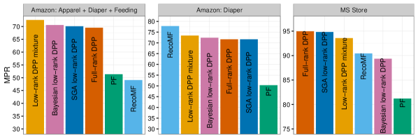
Figure 3: Mean Percentile Rank (MPR)

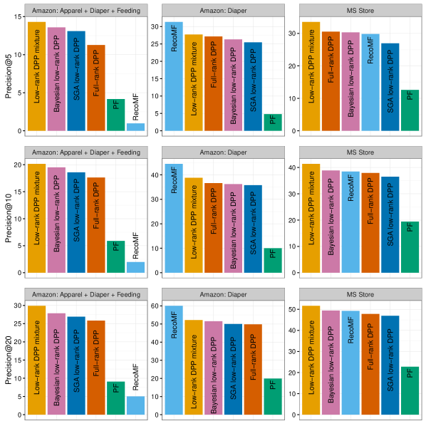
Figure 4: Precision@$k$

3.3 Metrics

In the following evaluation we consider three measures:

1. Mean Percentile Rank (MPR) - To compute this metric we rank the items according to their probabilities of completing the missing set $Y_{n-1}$. Namely, given an item $i$ from the candidates set $\mathcal{C}$, we denote by $p_{i}$ the probability $P\Large(Y_{n}\cup\{i\}|Y_{n-1}\Large)$. The Percentile Rank (PR) of the missing item $j$ is defined by $\text{PR}_{j}=\frac{\sum_{j^{\prime}\in\mathcal{C}}\mathbb{I}\Large(p_{j}\geq p_{j^{\prime}}\Large)}{|\mathcal{C}|}\times 100\%$, where $\mathbb{I}\Large(\cdot\Large)$ is an indicator function and $|\mathcal{C}|$ is the number of items in the candidates set. The Mean Percentile Rank (MPR) is the average PR of all the instances in the test-set: $\text{MPR}=\frac{\sum_{t\in\mathcal{T}}\text{PR}_{t}}{|\mathcal{T}|}$, where $\mathcal{T}$ is the set of test instances. MPR is a recall-oriented metric commonly used in studies that involve implicit recommendation data [13, 20]. $\text{MPR}=100$ always places the held-out item for the test instance at the head of the ranked list of predictions, while $\text{MPR}=50$ is equivalent to random selection.

2. Precision@$k$ - We define this metric as $\text{precision@}k=\frac{\sum_{t\in\mathcal{T}}\mathbb{I}[\text{rank}_{t}\leq k]}{|\mathcal{T}|}$, where $\text{rank}_{t}$ is the predicted rank of the held-out item for test instance $t$. In other words, precision@$k$ is the fraction of instances in the test set for which the predicted rank of the held-out item falls within the top $k$ predictions.

3. Popularity-weighted precision@$k$ - Datasets used to evaluate recommendation systems typically contain a popularity bias [30], where users are more likely to provide feedback on popular items. Due to this popularity bias, conventional metrics such as MPR and precision@$k$ are typically biased toward popular items. Using ideas from [30], we this metric as $\text{popularity-weighted precision@}k=\\ \frac{\sum_{t\in\mathcal{T}}w_{t}\mathbb{I}[\text{rank}_{t}\leq k]}{\sum_{t\in\mathcal{T}}w_{t}}$, where $w_{t}$ is the weight assigned to the held-out item for test instance $t$, defined as $w_{t}\propto\frac{1}{C(t)^{\beta}}$, where $C(t)$ is the number of occurrences of the held-out item for test instance $t$ in the training data, and $\beta\in[0,1]$. The weights are normalized, so that $\sum_{j\in\mathcal{Y}}w_{j}=1$. This popularity-weighted precision@$k$ measure assumes that item popularity follows a power-law. By assigning more weight to less popular items, for $\beta>0$, this measure serves to bias precision@$k$ towards less popular items. For $\beta=0$, we obtain the conventional precision@$k$ measure.

3.4 Predictive Performance

Figures 3 and 4 show the performance of each method and dataset for the MPR and precision@$k$ metrics. For these plots we selected the value of $K$, the number of trait dimensions, that provided the best performance on the precision@5 metric for each dataset. For the Amazon datasets, we use $K=30$ for the models that utilize low-rank DPPs and $K=40$ for the RecoMF and PF models. For the MS Store dataset, we use $K=60$ for the Bayesian low-rank DPP and low-rank DPP mixture models, $K=15$ for the SGA low-rank DPP model (the size of the largest observed basket in this dataset is 15 items), $K=40$ for RecoMF, and $K=90$ for PF.

We see that the low-rank DPP mixture model outperforms all other DPP models on precision@$k$ for all datasets, often by a sizeable margin. With the exception of the Amazon Diaper dataset, the low-rank DPP mixture model also provides significantly better precision@$k$ performance than competing non-DPP models. The low-rank DPP mixture model also provides consistently high MPR performance on all datasets. We attribute the strong predictive performance of the low-rank DPP mixture model to effective use of the increased capacity of this model afforded by the mixture components.

In Figure 5 we examine the performance of several models on precision@5 for the MS Store dataset as a function of the number of trait dimensions, $K$. We see that at even for $K=15$ the low-rank DPP mixture model is competitive with all other models, and at $K=60$ the mixture model significantly outperforms all other models, with a relative improvement of 10.6% over the score of the second-best model on this metric.

Figure 6 shows how the popularity-weighted precision@5 performance of three of the best performing models on the MS Store dataset varies as we adjust the value of the $\beta$ parameter used in the popularity-weighted precision@$k$ metric. Recall that $\beta$ controls the weight assigned to less popular items, and that for $\beta=0$ we obtain the standard precision@$k$ metric. For values of $\beta\leq 0.4$ the low-rank DPP mixture model provides leading or competitive performance, which shows that the increased model capacity provided by the mixture model allows for improved recommendations for less popular items in addition to popular items. For larger values of $\beta$, RecoMF provides the best performance. This behavior may be explained by the scheme for sampling negatives by popularity in RecoMF [26], which tends to improve recommendations for less popular items. The optimal setting of $\beta$ for approximating actual user satisfaction in a real-world application will depend on the particular application and user population. A small-scale user study conducted with the Netflix data [30] found that $\beta=0$ and $\beta=0.33$ best approximated user preferences for the application in that study.

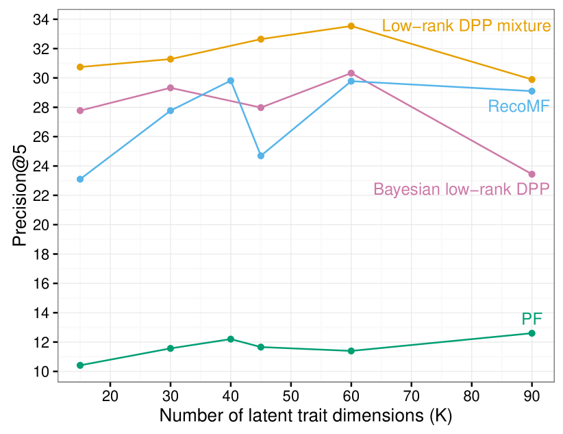
Figure 5: Precision@5 performance of the low-rank DPP mixture model, Bayesian low-rank DPP, RecoMF, and PF on the MS Store dataset as a function of the number of latent trait dimensions $K$.

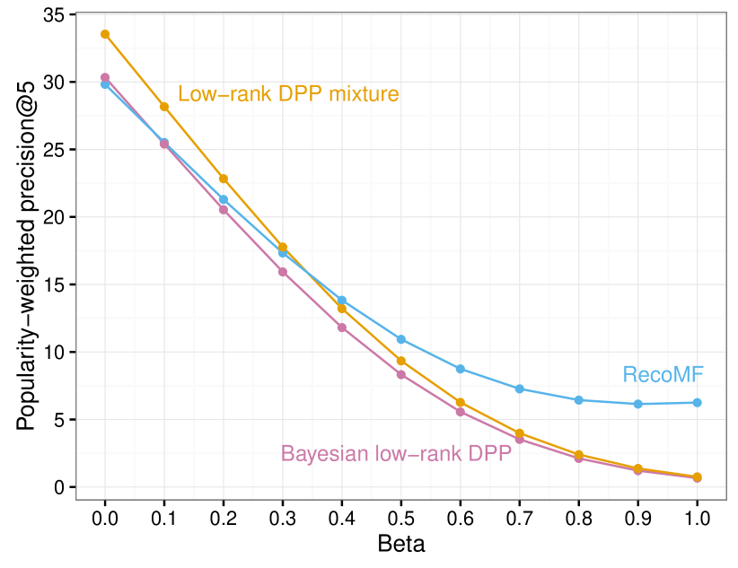
Figure 6: Popularity-weighted precision@5 performance of the low-rank DPP mixture model, Bayesian low-rank DPP, and RecoMF the MS Store dataset as a function of the $\beta$ parameter.

4 Related Work

Several algorithms for learning the DPP kernel matrix from observed data have been proposed [1, 11, 22]. Ref. [11] presented one of the first methods for learning a non-parametric form of the full-rank kernel matrix, which involves an expectation-maximization (EM) algorithm. In [22], a fixed-point optimization algorithm for full-rank DPP learning is described, called Picard iteration. Picard iteration has the advantage of being simple to implement and performing much faster than EM during training. Ref. [8] shows that a low-rank DPP model can be trained far more quickly than Picard iteration and therefore EM, while enabling much faster computation of predictions than is possible with any full-rank DPP model. A Bayesian low-rank DPP model is presented in [9], which provides robust regularization and does not require expensive hyperparameter tuning. The Bayesian low-rank DPP is the fundamental building block for our low-rank DPP mixture model.

Mixture models have been well known in the machine learning and statistics communities for some time. Ref. [6] describes an application of expectation maximization (EM) to mixture models. A variational Bayes implementation of mixture models is described in [2], while [24] describes the use of expectation propagation for mixture models. A Bayesian infinite Gaussian mixture model is described in [27], where an efficient MCMC algorithm is used for inference. Ref. [29] presents a mixture model for collaborative filtering, where user and items are clustered, while allowing each user and item to belong to multiple clusters to account for diversity in user interests and item aspects.

A number of approaches to the basket completion problem that we focus on in this paper have been proposed. Ref. [23] describes a user-neighborhood-based collaborative filtering method, which uses rating data in the form of binary purchases to compute the similarity between users, and then generates a purchase prediction for a user and item by computing a weighted average of the binary ratings for that item. A technique that uses logistic regression to predict if a user will purchase an item based on binary purchase scores obtained from market basket data is described in [19]. Additionally, other collaborative filtering approaches could be applied to the basket completion problem, such as the one-class matrix factorization model in [26] and Poisson factorization [12], as we illustrate in this paper.

5 Conclusions

We have presented a Bayesian low-rank DPP mixture model that represents observed subsets as a mixture of several component low-rank DPPs. Through the use of a stochastic MCMC learning algorithm that operates on minibatches of training data, we are able to avoid costly updates that would require full passes through the entire dataset as required by conventional MCMC learning algorithms. With an extensive evaluation on several real-world shopping basket datasets, we have shown that our mixture model effectively addresses the capacity constraints of conventional DPP models and provides significantly better predictive performance than these models. Our model also significantly outperforms state-of-the-art methods based on matrix factorization in many cases.

6 Acknowledgements

We thank Gal Lavee and Shay Ben Elazar for many helpful discussions. We thank Nir Nice for supporting this work.

References

- [1] R. H. Affandi, E. Fox, R. Adams, and B. Taskar. Learning the parameters of determinantal point process kernels. In ICML, pages 1224–1232, 2014.
- [2] C. M. Bishop. Pattern recognition and machine learning. 2006.
- [3] A. J. Chaney. Social Poisson factorization (SPF). https://github.com/ajbc/spf, 2015.
- [4] A. J. Chaney, D. M. Blei, and T. Eliassi-Rad. A probabilistic model for using social networks in personalized item recommendation. In RecSys, pages 43–50, 2015.
- [5] T. Chen, E. Fox, and C. Guestrin. Stochastic gradient hamiltonian monte carlo. In ICML, pages 1683–1691, 2014.
- [6] A. P. Dempster, N. M. Laird, and D. B. Rubin. Maximum likelihood from incomplete data via the em algorithm. Journal of the royal statistical society. Series B (methodological), pages 1–38, 1977.
- [7] S. Duane, A. D. Kennedy, B. J. Pendleton, and D. Roweth. Hybrid monte carlo. Physics letters B, 195(2):216–222, 1987.
- [8] M. Gartrell, U. Paquet, and N. Koenigstein. Low-rank factorization of determinantal point processes for recommendation. arXiv preprint arXiv:1602.05436, 2016.
- [9] M. Gartrell, U. Paquet, and N. Koenigstein. Bayesian low-rank determinantal point processes. In RecSys, 2016 (to appear).
- [10] J. Gillenwater. Approximate inference for determinantal point processes. PhD thesis, University of Pennsylvania, 2014.
- [11] J. A. Gillenwater, A. Kulesza, E. Fox, and B. Taskar. Expectation-maximization for learning determinantal point processes. In NIPS, pages 3149–3157, 2014.
- [12] P. Gopalan, J. M. Hofman, and D. M. Blei. Scalable recommendation with hierarchical Poisson factorization. In UAI, 2015.
- [13] Y. Hu, Y. Koren, and C. Volinsky. Collaborative filtering for implicit feedback datasets. In ICDM, pages 263–272, 2008.
- [14] H. Ishwaran and M. Zarepour. Dirichlet prior sieves in finite normal mixtures. Statistica Sinica, pages 941–963, 2002.
- [15] A. Kulesza and B. Taskar. Structured determinantal point processes. In NIPS, pages 1171–1179, 2010.
- [16] A. Kulesza and B. Taskar. Learning determinantal point processes. In UAI, 2011.
- [17] A. Kulesza and B. Taskar. Determinantal point processes for machine learning. Foundations and Trends in Machine Learning, 5(2-3):123–286, 2012.
- [18] J. T. Kwok and R. P. Adams. Priors for diversity in generative latent variable models. In NIPS, pages 2996–3004, 2012.
- [19] J.-S. Lee, C.-H. Jun, J. Lee, and S. Kim. Classification-based collaborative filtering using market basket data. Expert Systems with Applications, 29(3):700–704, 2005.
- [20] Y. Li, J. Hu, C. Zhai, and Y. Chen. Improving one-class collaborative filtering by incorporating rich user information. In CIKM, pages 959–968, 2010.
- [21] O. Macchi. The coincidence approach to stochastic point processes. Advances in Applied Probability, pages 83–122, 1975.
- [22] Z. Mariet and S. Sra. Fixed-point algorithms for learning determinantal point processes. In ICML, pages 2389–2397, 2015.
- [23] A. Mild and T. Reutterer. An improved collaborative filtering approach for predicting cross-category purchases based on binary market basket data. Journal of Retailing and Consumer Services, 10(3):123–133, 2003.
- [24] T. P. Minka. Expectation propagation for approximate bayesian inference. In UAI, pages 362–369, 2001.
- [25] R. M. Neal. Mcmc using hamiltonian dynamics. Handbook of Markov Chain Monte Carlo, 2:113–162, 2011.
- [26] U. Paquet and N. Koenigstein. One-class collaborative filtering with random graphs. In WWW, pages 999–1008, 2013.
- [27] C. E. Rasmussen. The infinite gaussian mixture model. In NIPS, volume 12, pages 554–560, 1999.
- [28] J. Rousseau and K. Mengersen. Asymptotic behaviour of the posterior distribution in overfitted mixture models. Journal of the Royal Statistical Society: Series B (Statistical Methodology), 73(5):689–710, 2011.
- [29] L. Si and R. Jin. Flexible mixture model for collaborative filtering. In ICML, pages 704–711, 2003.
- [30] H. Steck. Item popularity and recommendation accuracy. In RecSys, pages 125–132, 2011.