Eye Formation in Rotating Convection

Abstract

We consider rotating convection in a shallow, cylindrical domain. We examine the conditions under which the resulting vortex develops an eye at its core; that is, a region where the poloidal flow reverses and the angular momentum is low. For simplicity, we restrict ourselves to steady, axisymmetric flows in a Boussinesq fluid. Our numerical experiments show that, in such systems, an eye forms as a passive response to the development of a so-called eyewall, a conical annulus of intense, negative azimuthal vorticity that can form near the axis and separates the eye from the primary vortex. We also observe that the vorticity in the eyewall comes from the lower boundary layer, and relies on the fact the poloidal flow strips negative vorticity out of the boundary layer and carries it up into the fluid above as it turns upward near the axis. This process is effective only if the Reynolds number is sufficiently high for the advection of vorticity to dominate over diffusion. Finally we observe that, in the vicinity of the eye and the eyewall, the buoyancy and Coriolis forces are negligible, and so although these forces are crucial to driving and shaping the primary vortex, they play no direct role in eye formation in a Boussinesq fluid.

1 Introduction

One of the most striking features of atmospheric vortices, such as tropical cyclones, is that they often develop a so-called eye; a region of reversed flow in and around the axis of the vortex. Much has been written about eye formation, particularly in the context of tropical cyclones, but the key dynamical processes are still poorly understood (Pearce, 2005a; Smith, 2005; Pearce, 2005b). Naturally occurring vortices in the atmosphere are, of course, complicated objects, whose overall dynamics can be strongly influenced by, for example, planetary rotation, stratification, latent heat release through moist convection, and turbulent diffusion. Indeed the structure of eyes in tropical cyclones is almost certainly heavily influenced by both moist convection and stratification. However, the ubiquitous appearance of eyes embedded within large-scale vortices suggests that the underlying mechanism by which they first form may be independent (partially if not wholly) of such complexities. Indeed eye-like structures are observed in other atmospheric vortices such as tornadoes (Lugt, 1983, and references therein) or polar lows (Rasmussen & Turner, 2003), which are particularly interesting as they consist of large-scale convective cyclonic structures observed in high latitudes polar regions. To put the idea of a simple hydrodynamic mechanism to the test we consider what is, perhaps, the simplest system in which eyes may form; that of steady axisymmetric convection in a rotating Boussinesq fluid. We thus neglect the effects of stratification, and of moist convection. Our underlying assumption is that some atmospheric phenomena could be simple enough to be modelled in a uniform Boussinesq fluid. Indeed, a recent study by Guervilly et al. (2014) noted that Boussinesq convection can yield, as in the atmosphere, the formation of large scale cyclonic vortices.

In this work, we consider a rotating, cylindrical domain in which the lower surface is a no-slip boundary, the upper surface stress free, and the motion driven by a prescribed vertical flux of heat. In a frame of reference rotating with the lower boundary, the Coriolis force induces swirl in the convecting fluid, which in turn sets up an Ekman-like boundary layer on the lower surface. The primary flow in the vertical plane is then radially inward near the lower boundary and outward at the upper surface. As the fluid spirals inward, it carries its angular momentum with it (subject to some viscous diffusion) and this results in a region of particularly intense swirl near the axis. The overall flow pattern is as shown schematically in Figure 1.

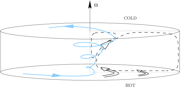
Figure 1: Cartoon showing the global flow pattern in rotating convection. The motion in the vertical plane consists of the primary vortex, the eye-wall and the eye, while the azimuthal motion consists of regions of high angular momentum near the axis and low (or even negative) angular momentum at larger radii (the vertical axis is stretched by a coefficient $5$ for readability).

In the vertical plane the primary vortex has a clockwise motion, and so has positive azimuthal vorticity. If an eye forms, however, its motion is anticlockwise in the vertical plane (Figure 1), and so the eye is associated with negative azimuthal vorticity. A key question, therefore, is: where does this negative vorticity come from? We shall show that it is not generated by buoyancy, since such forces are locally too weak. Nor does it arise from so-called vortex tilting, despite the local dominance of this process, because vortex tilting cannot produce any net azimuthal vorticity. Rather, the eye acquires its vorticity from the surrounding fluid by cross-stream diffusion, and this observation holds the key to eye formation in our simple system.

The region that separates the eye from the primary vortex is usually called the eyewall, and we shall see that this thin annular region is filled with intense negative azimuthal vorticity. So eye formation in our model problem is really all about the dynamics of creating an eyewall. In this paper we use numerical experiments to investigate the processes by which eyes and eyewalls form in our model system. We identify the key dynamical mechanisms and force balances, and provide a simple criterion which needs to be met for an eye to form.

2 Problem Specification and Governing Equations

We consider the steady flow of a Boussinesq fluid in a rotating, cylindrical domain of height $H$ and radius $R$, with $R\gg H$. The aspect ratio is denoted as $\varepsilon=H/R$. The flow is described in cylindrical polar coordinates, $(r,\phi,z)$, where the lower surface, $z=0$, and the outer radius, $r=R$, are no-slip boundaries. The upper surface, $z=H$, is impermeable but stress free. The motion is driven by buoyancy with a fixed upward heat flux maintained between the surfaces $z=0$ and $z=H$. In static equilibrium there is a uniform temperature gradient, ${\rm d}{\rm T}_{0}/{\rm d}z=-\beta$. We decompose ${\rm T}={\rm T}_{0}(z)+\theta$, where $\theta$ is the perturbation in temperature from the linear profile. In order to maintain a constant heat flux the thermal boundary conditions on the surfaces $z=0$ and $z=H$ are $\partial\theta/\partial z=0$, while the outer radial boundary is thermally insulating, $\partial\theta/\partial r=0$. The flow domain and boundary conditions are summarised in Figure 2.

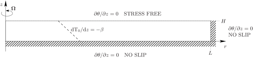
Figure 2: Flow domain and boundary conditions.

We adopt a frame of reference that rotates with the boundaries. Denoting $\Omega$ the background rotation rate, g the gravitational acceleration, $\nu$ the kinematic viscosity of the fluid, $\kappa$ its thermal diffusivity, and $\alpha$ its thermal expansion coefficient, the governing equations are

$$\frac{{\rm D}\mbox{\bf u}}{{\rm D}t}=-\frac{1}{\rho_{0}}\,\mbox{\boldmath$\nabla$}p-2\mbox{\boldmath$\Omega$}\times\mbox{\bf u}+\nu\,\mbox{\boldmath$\nabla$}^{2}\mbox{\bf u}-\alpha\,\theta\,\mbox{\bf g}\,,\qquad\mbox{\boldmath$\nabla$}\cdot\mbox{\bf u}=0\,, e f$$ (1,)

and

$$\frac{{\rm D}\theta}{{\rm D}t}=\kappa\,\mbox{\boldmath$\nabla$}^{2}\theta+\beta\,{\rm u}_{z}\,, h$$ (1)

(e.g. Chandrasekhar, 1981; Drazin, 2002). We further restrict ourselves to axisymmetric motion, so that we may decompose the velocity field into poloidal and azimuthal velocity components, $\mbox{\bf u}_{p}=({\rm u}_{r},0,{\rm u}_{z})$ and $\mbox{\bf u}_{\phi}=(0,{\rm u}_{\phi},0)$, which are separately solenoidal. The azimuthal component of (2$a$) then becomes an evolution equation for the specific angular momentum in the rotating frame, $\Gamma=r{\rm u}_{\phi}$,

$$\frac{{\rm D}\Gamma}{{\rm D}t}=-2r\,\Omega\,{\rm u}_{r}+\nu\mbox{$\nabla_{\star}^{2}$}(\Gamma)\,,$$ (2)

where

$$\mbox{$\nabla_{\star}^{2}$}=r\frac{\partial}{\partial r}\left(\frac{1}{r}\frac{\partial}{\partial r}\right)+\frac{\partial^{2}}{\partial z^{2}}$$

is the Stokes operator. Moreover the curl of the poloidal components yields an evolution equation for the azimuthal vorticity, $\mbox{\boldmath$\omega$}_{\phi}=\mbox{\boldmath$\nabla$}\times\mbox{\bf u}_{p}\,,$

$$\frac{{\rm D}}{{\rm D}t}\left(\frac{\omega_{\phi}}{r}\right)=\frac{\partial}{\partial z}\left(\frac{\Gamma^{2}}{r^{4}}\right)+\frac{2\,\Omega}{r}\frac{\partial{\rm u}_{\phi}}{\partial z}-\frac{\alpha g}{r}\,\frac{\partial\theta}{\partial r}+\frac{\nu}{r^{2}}\mbox{$\nabla_{\star}^{2}$}\left(r\omega_{\phi}\right)\,.$$ (3)

We recognize the curl of the Coriolis, buoyancy and viscous forces on the right of (3). The axial gradient in $\Gamma^{2}/r^{4}$ is, perhaps, a little less familiar as a source of azimuthal vorticity. However, this arises from the contribution of $\mbox{\boldmath$\nabla$}\times\left(\mbox{\bf u}_{\phi}\times\mbox{\boldmath$\omega$}_{p}\right)\,,$ where $\mbox{\boldmath$\omega$}_{p}=\mbox{\boldmath$\omega$}-\mbox{\boldmath$\omega$}_{\phi}\,,$ to the vorticity equation and represents the self-advection (spiralling up) of the poloidal vorticity-lines by axial gradients in swirl (e.g. Davidson, 2013). The scalar equations (2) and (3) are formally equivalent to (2$a$), with $\Gamma$ and $\omega_{\phi}$ uniquely determining the instantaneous velocity distribution. Finally, it is convenient to introduce the Stokes stream-function, $\psi$, which is defined by $\mbox{\bf u}_{p}=\mbox{\boldmath$\nabla$}\times\left[\left(\psi/r\right)\mbox{\bf e}_{\phi}\right]$ and related to the azimuthal vorticity by $r\omega_{\phi}=-\mbox{$\nabla_{\star}^{2}$}\psi\,.$

3 Global Dynamics

We perform numerical simulations in the form of an initial value problem which is run until a steady state is reached. We solve equations (1$h$), (2) and (3) in which the length has been scaled with the height $H$ of the system, the time with $\Omega^{-1}\,,$ and the temperature with $H\beta\,.$ The dimensionless control parameters of the system are the Ekman number ${\rm E}={\nu}/{\Omega H^{2}}\,,$ the Prandtl number ${\rm Pr}={\nu}/{\kappa}\,,$ and the Rayleigh number ${\rm Ra}={\alpha g\beta H^{4}}/{\nu\kappa}\,.$

We use second-order finite differences and an implicit second-order backward differentiation (BDF2) in time. The number of radial and axial cells is $1000\times 500$, and in each simulation grid resolution studies were undertaken to ensure numerical convergence. The aspect ratio of the computational domain is set at $\varepsilon=0.1$, a ratio inspired by tropical storms (for which $H\simeq 10$km, and $R\simeq 100$km). The Ekman number ${\rm E}$ is set to $0.1$, which is a sensible turbulent estimate for tropical cyclones. The values of $\Pr$ and ${\rm Ra}$ will be varied through this study to control the strength of the convection.

We shall consider flows in which the local Rossby number ${\rm Ro}={\rm u}_{\phi}/{\Omega H}\,,$ is of the order unity or less at large radius, $r\simeq L\,,$ but is large near the axis, $r\simeq H\,,$ which is not untypical of a tropical cyclone and turns out to be the regime in which an eye and eyewall form in our numerical simulations. We shall also take a suitably defined Reynolds number, ${\rm Re}\,,$ to be considerably larger than unity, though not so large that the laminar flow becomes unsteady. A moderately large Reynolds number also turns out to be crucial to eye formation.

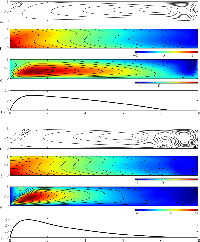
Figure 3: Steady state solution in the $(r,z)$-plane for the parameters ${\rm Pr}=0.5$ and ${\rm Ra}=1.5\times 10^{4}$ in (a–d), and for ${\rm Pr}=0.1$ and ${\rm Ra}=2\times 10^{4}$ in (e–h). (a,e) The stream-function distribution, (b,f) the total temperature ${\rm T}={\rm T}_{0}(z)+\theta$, (c,g) the azimuthal velocity, ${\rm u}_{\phi}$, (d,h) the radial variation of ${\rm Ro}$.

In order to focus thoughts, let us start by considering two specific cases: $\Pr=0.5\,,\,\,{\rm Ra}=1.5\times 10^{4}\,,$ and $\Pr=0.1\,,\,\,{\rm Ra}=2\times 10^{4}\,.$ These two cases are represented in Fig. 3. In both cases, the primary flow in the vertical plane is radially inward near the lower boundary and outward at the upper surface. The steady state stream-function distributions are shown in Fig. 3a,e. It is evident that in both cases an eye has formed near the axis, but it is much more pronounced in the later case. Fig. 3b,f show the corresponding distributions of total temperature. The poloidal flow sweeps heat towards axis at low values of $z$, causing a build-up of heat near the axis with a corresponding cooler region at larger radii. The resulting negative radial gradient in ${\rm T}$ drives the main poloidal vortex, ensuring that it has positive azimuthal vorticity in accordance with (3). Fig. 3c,g present the distributions of the azimuthal velocity. The Coriolis force induces swirl in the convecting fluid. As the fluid spirals inward, it carries its angular momentum with it (subject to some viscous diffusion) and this results in a region of particularly intense swirl near the axis. It also shows a substantial region of negative (anti-cyclonic rotation) at large radius, something that is also observed in tropical cyclones (e.g. Frank, 1977). In order to quantify the strength of the azimuthal flow, we introduce a Rossby number which is a function of radius ${\rm Ro}(r)={\left({\rm u}_{\phi}\right)_{\rm max}}/{\Omega H}\,,$ where $\left({\rm u}_{\phi}\right)_{\rm max}$ is the maximum value of azimuthal velocity at any one radial location. The Rossby number as a function of radius is represented in Fig. 3d,h. The eye is obtained when the local Rossby number, is of the order unity at large radius, $r\simeq L$, but is large near the axis, $r\simeq H$. Given the increase of ${\rm Ro}$ near the axis, the Coriolis force can be neglected in the vicinity of the eye. Note that, in the second case (Fig. 3e,f,g,h), the Rossby number is much larger, and the eye much more pronounced than in the first case (Fig. 3a,b,c,d).

To summarise, in both cases, the buoyancy force evidently drives motion in the poloidal plane, which in turn induces spatial variations in angular momentum, $\Gamma$, through the Coriolis force, $2\Omega r{\rm u}_{r}$, in (2). The flow spirals radially inward along the lower boundary and outward near $z=H$, as shown in Fig. 1. The Coriolis force then ensures that the angular momentum, $\Gamma$, rises as the fluid spirals inward along the bottom boundary, but falls as it spirals back out along the upper surface towards $r=L$. The swirl of the flow as it approaches the axis is thus controled both by the Ekman number and by the aspect ratio of the domain. With our choice of the parameters, particularly high levels of azimuthal velocity built up near the axis, with a correspondingly large value of ${\rm Ro}$ in the vicinity of the eyewall. In some sense, then, the global flow pattern is both established and shaped by the buoyancy and Coriolis forces, yet, as we shall discuss, these forces are negligible in the viscinity of the eye.

4 Global Versus Local Dynamics

4.1 The anatomy of eyewall formation

The large value of ${\rm Ro}$ near the axis means that the Coriolis force is locally negligible in the region where the eye and eyewall form, and it turns out that this is true also of the buoyancy force in our Boussinesq simulations. Thus the very forces that establish the global flow pattern play no significant role in the local dynamics of the eye. It is worth considering, therefore, the simplified version of (2) and (3) which operate near the axis,

$$\frac{{\rm D}\Gamma}{{\rm D}t}\simeq\nu\mbox{$\nabla_{\star}^{2}$}(\Gamma)\,,$$ (4)

and

$$\frac{{\rm D}}{{\rm D}t}\left(\frac{\omega_{\phi}}{r}\right)\simeq\frac{\partial}{\partial z}\left(\frac{\Gamma^{2}}{r^{4}}\right)+\frac{\nu}{r^{2}}\mbox{$\nabla_{\star}^{2}$}\left(r\omega_{\phi}\right)\,.$$ (5)

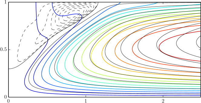
Figure 4: Contours of constant angular momentum (color) superimposed on the streamlines (black) in the inner quarter of the flow domain ($(r,z)$-plane), for $\Pr=0.1$ and ${\rm Ra}=2\times 10^{4}$.

The eye is characterised by anticlockwise motion in the $(r,z)$-plane ($\omega_{\phi}<0$), in contrast to the global vortex that is clockwise ($\omega_{\phi}>0$). It is also characterised by low levels of angular momentum. A natural question to ask, therefore, is where this negative azimuthal vorticity comes from. Since $\Gamma$ is small in the eye, $\omega_{\phi}/r$ is locally governed by a simple advection diffusion equation in which the source term is negligible, and so the negative azimuthal vorticity in the eye has most probably diffused into the eye from the eyewall. This kind of slow cross-stream diffusion of vorticity into a region of closed streamlines is familiar from the Prandtl-Batchelor theorem (Batchelor, 1956), and in this sense the eye is a passive response to the accumulation of negative $\omega_{\phi}$ in the eyewall. If this is substantially true, and we shall see that it is, then the key to eye formation is the generation of significant levels of negative azimuthal vorticity in the eyewall, and so the central questions we seek to answer is how, and under what conditions, the eyewall acquires this negative vorticity.

Given that the Reynolds number is large, it is tempting to consider the inviscid limit and attribute the growth of negative $\omega_{\phi}$ to the first term on the right of (5). That is, axial gradients in $\Gamma$ can act as a local source of azimuthal vorticity, and indeed this mechanism has been invoked by previous authors in the context of tropical cyclones (e.g. Pearce, 2005a; Smith, 2005; Pearce, 2005b). The idea is that, in steady state, if viscous diffusion is ignored in the vicinity of the eyewall, (4) and (5) locally reduce to

$$\Gamma=\Gamma\left(\psi\right)\,,$$ (6)

and

$$\mbox{\bf u}\cdot\mbox{\boldmath$\nabla$}\left(\omega_{\phi}/r\right)=\frac{\partial}{\partial z}\left(\frac{\Gamma^{2}}{r^{4}}\right)=-2\frac{\Gamma\Gamma^{\prime}\left(\psi\right)}{r^{3}}{\rm u}_{r}\,.$$ (7)

To the extent the viscosity can be ignored, $\Gamma\left(\psi\right)$ increases to a maximum at roughly mid-height, where $\psi$ is a maximum, and then drops off as we approach the upper boundary. Thus $\Gamma^{\prime}\left(\psi\right)>0$, and so according to (7) positive vorticity is induced as the streamlines curve inward and upward, while negative vorticity is created after the streamlines turn around and ${\rm u}_{r}$ reverses sign. Since the eyewall is associated with the upper region, where the flow is outward, it is natural to suppose that the negative vorticity in the eyewall arises from precisely this process. However, in the case of a Boussinesq fluid, this term cannot produce any net negative azimuthal vorticity in the eyewall, essentially because the term on the right of (7) is a divergence. To see why this is so, we rewrite (7) as

$$\mbox{\boldmath$\nabla$}\cdot\left[\left(\omega_{\phi}/r\right)\mbox{\bf u}\right]=\mbox{\boldmath$\nabla$}\cdot\left[\left(\Gamma^{2}/r^{4}\right)\mbox{\bf e}_{z}\right]\,,$$ (8)

and integrate this over a control volume in the form of a stream-tube in the $r-z$ plane composed of two adjacent streamlines that pass through the eyewall. If the stream-tube within the control volume starts and ends at a fixed radius somewhat removed from the eyewall, then the right-hand divergence integrates to zero. The flux of vorticity into the control volume (the stream-tube) is therefore the same as that leaving. In short, the azimuthal vorticity generated in the lower regions where the streamlines curve inward and upward is exactly counterbalanced by the generation of negative vorticity in the upper regions where the flow is radially outward. Such a process cannot result in any negative azimuthal vorticity in the eyewall. Returning to (5) we conclude that the only possible source of net negative vorticity in the eyewall is the viscous term, and this drives us to the hypothesis that the negative vorticity in the eyewall has its origins in the lower boundary layer. That is, negative azimuthal vorticity is generated at the lower boundary and then advected up into eyewall where it subsequently acts as the source for a slow cross-stream diffusion of negative vorticity into the eye. Of course, as the streamlines pass up into, and then through, the eyewall there is also a generation of first positive and then negative azimuthal vorticity by the axial gradients in $\Gamma^{2}/r^{4}$, but these two contributions exactly cancel, and so cannot contribute to the negative vorticity in the eyewall.

The above description is put to the test in Fig. 4 to Fig. 7. A more detailed view of the angular momentum distribution and streamlines in the region adjacent to the eye and eyewall is provided in Fig. 4. In the region to the right of the eye, the contours of constant angular momentum are roughly aligned with the streamlines, in accordance with (6). Note that, although the contours of constant $\Gamma$ roughly follow the streamlines, the two sets of contours are not entirely aligned. This is mostly a result of cross-stream diffusion, particularly near the eyewall, although it also partially arises from the (relatively weak) Coriolis force.

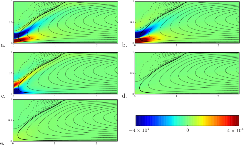
Figure 5: Colour maps of the distribution of the various forces in the azimuthal vorticity equation (3) in the inner part of the flow domain ($(r,z)$-plane): (a) the convective derivative of azimuthal vorticity; (b) the term associated with axial gradients in $\Gamma$; (c) diffusion; (d) the Coriolis term; and (e) buoyancy. Parameters: $\Pr=0.1\,,\ {\rm Ra}=2\times 10^{4}$.

Fig. 5 shows the distribution and relative magnitudes of the various forces in the azimuthal vorticity equation across the inner part of the flow domain. The buoyancy and Coriolis terms, though important for the large scale dynamics, are locally negligible (panels 5(d) and 5(e)), while diffusion is largely limited to the boundary layer, the eyewall, and a region near the axis where the flow turns around (panel 5c). Note also that $\partial\left(\Gamma^{2}/r^{4}\right)/\partial z$ is small within the eye (panel 5b) but there are intense regions of equal and opposite $\partial\left(\Gamma^{2}/r^{4}\right)/\partial z$ below the eyewall, which are matched by corresponding regions of equal and opposite $\mbox{\bf u}\cdot\mbox{\boldmath$\nabla$}\left(\omega_{\phi}/r\right)$ in panel 5a. These figures appear to validate that (5) is the relevant equation in this domain. It is interesting that the very forces that shape the global flow, i.e. the Coriolis and buoyancy forces, play no role in the vicinity of the eye.

This can be further highlighted by introducing the variable $\tau$, defined as a parametric coordinate along an iso-$\psi$. It corresponds to the position at a given time $\tau$ for a particle advected along a streamline; it stems from $\left(\left.{{\rm d}z}/{{\rm d}\tau}\right)\right|_{\psi={\rm cst}}={\rm u}_{z}\,.$ The constant of integration is set such that $\tau=0$ for the maximum of $\omega_{\phi}/r$. Fig. 6 shows forces in the azimuthal vorticity equation, as a function of position on the streamline that passes through the centre of the eyewall (thick streamline in Fig. 5). To first order there is an approximate balance between the advection of $\omega_{\phi}/r$ and $\partial\left(\Gamma^{2}/r^{4}\right)/\partial z$, though there is a significant contribution from the diffusion of vorticity within the eyewall. Both the Coriolis and buoyancy terms are completely negligible. In short, the force balance is that of (5).

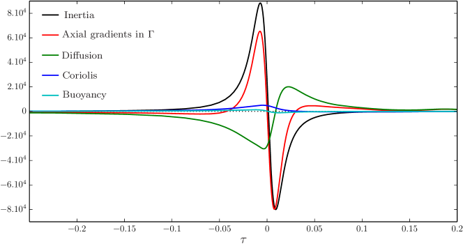
Figure 6: The variation of the terms in the azimuthal vorticity equation (3) with position on the streamline that passes through the centre of the eyewall. The convective derivative on the left-hand side of (3) is black, the term associated with axial gradients in $\Gamma$ is red, the viscous term is green, and the Coriolis and buoyancy terms (blue and light blue) are indistinguishable from the $x$-axis. Parameters: $\Pr=0.1\,,\ {\rm Ra}=2\times 10^{4}$.

The main features of the eyewall are most clearly seen in Fig. 7a, which shows the distribution of azimuthal vorticity, $\omega_{\phi}/r$, superimposed on the streamlines. The exceptionally strong levels of azimuthal vorticity in and around the eyewall is immediately apparent, and indeed it is tempting to define the eyewall as the outward sloping region of strong negative azimuthal vorticity which separates the eye from the primary vortex. There are two other important features of Fig. 7a. First, a large reservoir of negative azimuthal vorticity builds up in the lower boundary layer, as it must. Second, between the lower boundary and the eyewall there is a region of intense positive azimuthal vorticity. Fig. 7b. shows the variation of $\omega_{\phi}/r$ along the streamline that passes through the centre of the eyewall, as indicated by the thick black line in Fig. 7a. As the streamline passes along the bottom boundary layer, $\omega_{\phi}/r$ becomes progressively more negative. There is then a sharp rise in $\omega_{\phi}/r$ as the streamline pulls out of the boundary layer and into a region of positive $\partial\Gamma/\partial z$, followed by a corresponding drop as the streamline passes into the region of negative $\partial\Gamma/\partial z$. Crucially, the rise and subsequent fall in $\omega_{\phi}/r$ caused by axial gradients in angular momentum exactly cancel, and so the fluid emerges into the eyewall with the same level of vorticity it had on leaving the boundary layer.

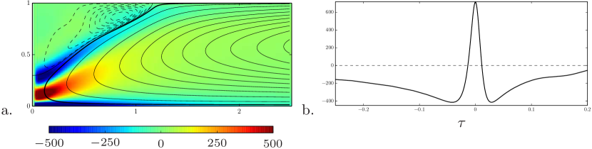
Figure 7: (a) Colour map of $\omega_{\phi}/r$ superimposed on the streamlines in the inner quarter of the domain ($(r,z)$-plane). (b) The variation of $\omega_{\phi}/r$ along the streamline that passes through the centre of the eyewall (as indicated by the thick black line in a). Parameters: $\Pr=0.1\,,\ {\rm Ra}=2\times 10^{4}$.

Finally we consider in Fig. 8 and Fig. 9 the distribution of the various contributions to the angular momentum equation (2). Fig. 8 shows the variation of these terms along the streamline that passes through the centre of the eyewall, as indicated by the thick black line in Figure 5. As before, the origin for the horizontal axis is taken to be the innermost point on the streamline. Clearly, within the eyewall there is a leading-order balance between the advection and diffusion of angular momentum, in accordance with the approximate equation (4), although the Coriolis torque is not entirely negligible. However, within the boundary layer ahead of the eyewall the force balance is quite different, with the Coriolis and viscous forces being in approximate balance, the convective growth of angular momentum being small.

A similar impression may be gained from Fig. 9 which shows, for the inner quarter of the flow domain, the distribution of the various contributions to equation (2). The panel (a) is the convective derivative of $\Gamma$ on the left of (2), the panel (b) is the diffusion term on the right, and the panel (c) is the Coriolis torque. Clearly, the positive Coriolis torque acting near the bottom boundary layer is largely matched by local cross-stream diffusion, the convective growth of angular momentum being small. The negative Coriolis torque acting on the outflow near the upper surface is mostly balanced by $\mbox{\bf u}\cdot\mbox{\boldmath$\nabla$}\Gamma$, resulting in a fall in $\Gamma$. Within the eyewall, the force balance is quite different, since there is a leading-order balance between the advection and diffusion of angular momentum, and the Coriolis torque is very weak. This confirms our previous observations in Fig. 5, and is in accordance with the approximate equation (4).

To summarise, in this particular simulation the eyewall that separates the eye from the primary vortex is characterised by high levels of negative azimuthal vorticity. That vorticity comes not from the term $\partial(\Gamma^{2}/r^{4})/\partial z$, despite its local dominance, but rather from the boundary layer at $z=0$. The eye then acquires its negative vorticity by cross-stream diffusion from the eyewall, in accordance with the Prandtl-Batchelor theorem. Although the global flow is driven and shaped by the buoyancy and Coriolis forces, these play no significant dynamical role in the vicinity of the eye and eyewall. As we shall see, these dynamical features characterise all of our simulations that produce eyes.

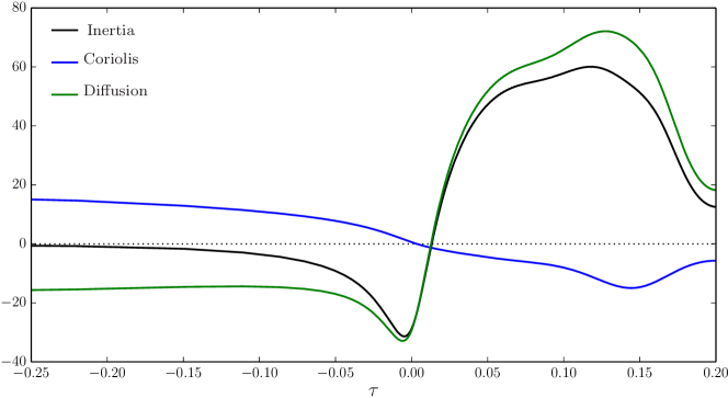
Figure 8: The variation of the various torques in the angular momentum equation (2) with position on the streamline that passes through the centre of the eyewall. The convective derivative on the left-hand side of (2) is black, the viscous diffusion term is green, and the Coriolis term is blue.

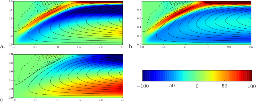
Figure 9: The spatial distribution of the various torques in the angular momentum equation in the inner part of the flow domain ($(r,z)$-plane) : (a) the convective derivative of $\Gamma$, (b) the diffusion term on the right, and (c) the Coriolis torque. Parameters: $\Pr=0.1\,,\ {\rm Ra}=2\times 10^{4}$.

4.2 A comparison of vortices that do and do not form eyes

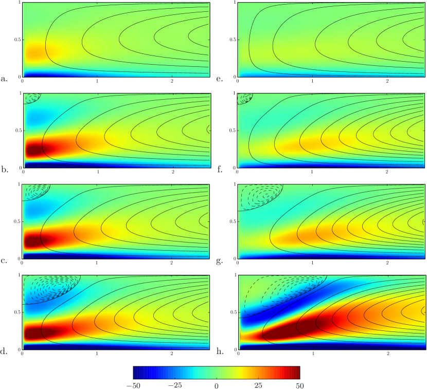
Figure 10: Colour map of $\omega_{\phi}/r$ superimposed on the streamlines in the inner quarter of the domain ($(r,z)$-plane), for ${\rm Pr}=0.3$ and (a) ${\rm Ra}=2\times 10^{3}$, (b) ${\rm Ra}=5.5\times 10^{3}$, (c) ${\rm Ra}=6\times 10^{3}$, (d) ${\rm Ra}=9\times 10^{3}$, and for ${\rm Pr}=0.1$ and (e) ${\rm Ra}=10^{3}$, (f) ${\rm Ra}=1.7\times 10^{3}$, (g) ${\rm Ra}=2\times 10^{3}$, (h) ${\rm Ra}=5\times 10^{3}\,.$ The colour code is the same on all graphs.

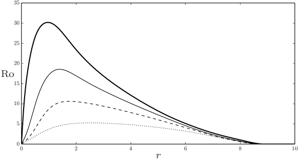
Figure 11: The radial variation of ${\rm Ro}$, for the cases with $\Pr=0.1$ and ${\rm Ra}=10^{3}$ (dotted), ${\rm Ra}=2\times 10^{3}$ (dashed), ${\rm Ra}=5\times 10^{3}$ (thin solid) and ${\rm Ra}=2\times 10^{4}$ (thick solid).

Let us now compare numerical simulations at given values of the Prandtl number ($\Pr=0.3$ and $\Pr=0.1$) and varying Rayleigh numbers. Figure 10 shows the stream-function distribution. Clearly, eyes form in Fig. 10b,c,d,f,g,h. From Table 1 and Fig. 11, we see that the peak value of ${\rm Ro}$ is of the order of $10$ or larger in those cases where an eye forms, which is typical of an atmospheric vortex.

Table 1: Sample of numerical results, ${\rm Re}$ is defined by equation (9).

${\rm Ra}$	max$({\rm Ro})\!\!\!$	${\rm Re}$	Eye?
$\varepsilon=0.1$  ${\rm E}=0.1$  $\Pr=0.1$
1000	5.27	17.78	0
1500	8.32	29.93	0
1650	9.07	33.2	0
1700	9.3	34.27	1
1750	9.53	35.32	1
1800	9.76	36.37	1
2000	10.61	40.44	1
5000	18.56	86.02	1
20000	30.18	178	1
$\varepsilon=0.1$  ${\rm E}=0.1$  $\Pr=0.3$
2000	3.39	18.98	0
4000	5.79	30.48	0
5000	6.72	34.75	0
5500	7.14	36.66	1
6000	7.54	38.44	1
8000	8.96	44.59	1
9000	9.59	47.17	1
$\varepsilon=0.1$  ${\rm E}=0.1$  $\Pr=0.5$
6000	4.38	24.33	0
8000	5.27	28.73	0
10000	6.04	32.53	0
11500	6.58	35.11	0
12000	6.75	35.91	0
13000	7.08	37.46	1
15000	7.72	40.09	1
$\varepsilon=0.1$  ${\rm E}=0.1$  $\Pr=0.8$
8000	3.17	18.19	0
15000	4.81	26.2	0
25000	6.5	35.04	0
27000	6.8	36.59	0
28700	7.04	37.86	0
29300	7.13	38.3	0
29400	7.13	38.37	0
29500	7.15	38.44	0
29650	7.17	38.55	1
29700	7.18	38.58	1

The clearest way to distinguish those flows where an eye forms from those in which it does not is to examine the spatial distribution of the azimuthal vorticity, shown in Fig. 10. In cases with a strong eye (Fig. 10d,h), the distribution of $\omega_{\phi}/r$ is similar to that in Fig. 7a, with regions of strong negative vorticity in the boundary layer and eyewall, and a patch of intense positive vorticity below the eyewall. The negative eyewall vorticity has its origins in the boundary layer, with the moderately large Reynolds number allowing this vorticity to be swept up from the boundary layer into the eyewall. Note, in particular, that the magnitude of vorticity in the eyewall is similar to that in the boundary layer.

Turning to Fig. 10b,c,f,g, which are somewhat marginal, in the sense that the eye is small, we see that overall flow pattern is similar, but that the negative eyewall vorticity is now relatively weak, and in particular significantly weaker than that in the boundary layer. It seems likely that the eyewall vorticity is relatively weak because advection has to compete with cross-stream diffusion as the poloidal flow tries to sweep the boundary layer vorticity up in the eyewall. In short, much of the boundary layer vorticity is lost to the surrounding fluid by diffusion before the fluid reaches the eyewall. Since the eye acquires its vorticity from the eyewall via cross-steam diffusion, the relative weakness of the eyewall vorticity explains the weakness of the resulting eye.

In Fig. 10a,e, where no eye forms, no region of intense negative vorticity forms as the poloidal flow turns and ${\rm u}_{r}$ changes sign. Since there is still a reservoir of negative vorticity in the boundary layer, and the basic shape of the primary vortex is unchanged, we conclude that the Reynolds number is now too low for the flow to effectively sweep the boundary-layer vorticity up into the fluid above.

The comparison of Fig. 10b and Fig. 10f reveals of decreasing the Prandtl number yields stronger inertial effects and thus allows to sustain an eye at lower Rayleigh numbers.

4.3 A criterion for eye formation

The mechanism introduced above works only if the Reynolds number, ${\rm Re}$, is sufficiently large, so that the flow can lift the vorticity out of the boundary layer and into the eyewall before is disperses though viscous diffusion. This suggests that there is a threshold value in ${\rm Re}$ that must be met in order for an eyewall to form. We take this Reynolds number to be based on the maximum value of the inward radial velocity, $|{\rm u}_{r}|_{\rm max}$, at a radial location just outside the region containing the eye and eyewall. We (somewhat arbitrarily) choose the radial location at which $|{\rm u}_{r}|_{\rm max}$ is evaluated to be $r=H$, which does in fact lie just outside the eyewall. Thus ${\rm Re}$ is defined as

$${\rm Re}=\frac{|{\rm u}_{r} |_{\rm max}H}{\nu}\,,$$ (9)

and is chosen to be larger than unity, though not so large that the flow becomes unsteady.

The logic behind this specific definition of ${\rm Re}$ is that the poloidal velocity field in the vicinity of the eyewall is dominated, via the Biot-Savart law, by the flux of vorticity up through the eyewall. This, in turn, is related to the flux of negative azimuthal vorticity in the boundary layer just outside the eyewall region. However, evaluating this flux by integrating $|\omega_{\phi}|$ up through this boundary layer from to the point where $|\omega_{\phi}|=0$ simply gives $|{\rm u}_{r}|_{\rm max}\,.$ We conclude, therefore, that $|{\rm u}_{r}|_{\rm max}$ is the characteristic poloidal velocity in the vicinity of the eyewall, and that ${\rm Re}$ is therefore a suitable measure of the ratio of advection to diffusion of azimuthal vorticity in this region.

Note that, since the buoyancy and Coriolis forces are negligible in the vicinity of the eye and eyewall, the criterion for a transition from eye formation to no eye cannot be controlled explicitly by ${\rm E}$ or ${\rm Ra}$, but rather must depend on ${\rm Re}$ only. So, to study the transition in the numerical experiments, we selected values of ${\rm E}$, ${\rm Pr}$ and ${\rm Ra}$ that yield steady flows with moderately large Reynolds numbers, as defined by (9), and with ${\rm Ro}$ somewhat larger than unity in the vicinity of the axis, i.e. those conditions which are conducive to eye formation. The values of ${\rm Re}$ obtained from our numerical experiments are reported in Figure. 12 and some are listed in Table 1.

A reasonably large Reynolds number also turns out to be crucial to eye formation. There is indeed a critical value of ${\rm Re}$ below which an eye cannot form. Fig. 12a shows ${\rm Re}$ as a function of ${\rm Ra}$ and $\Pr$, with the open symbols representing cases where an eye forms, and closed symbols those where there is no eye. There is clear evidence that the two classes of flow are separated by a plateau in ${\rm Re}$. This is confirmed by the two-dimensional plots of ${\rm Re}$ versus ${\rm Ra}$ and ${\rm Re}$ versus $\Pr$ given in panels (b) and (c). For the model and parameter regime considered here, the transition occurs at ${\rm Re}\simeq 37$, as indicated by the horizontal grey surface in Fig. 12a and the corresponding lines in Fig. 12b,c.

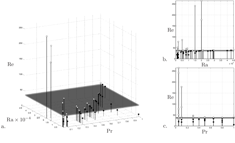
Figure 12: ${\rm Re}$, as defined by (9), as a function of (a) ${\rm Ra}$ and $\Pr$, (b) ${\rm Ra}$ and (c) $\Pr$. Open symbols represent cases where an eye forms, and closed symbols those where there is no eye.

5 Conclusions

We considered axisymmetric steady Boussinesq convection. In the vertical plane the primary vortex has a clockwise motion, and so has positive azimuthal vorticity. In the elongated and rotating domain considered here, the flow is characterised by a strong swirl as it approaches the axis. We have shown that, in this configuration, for sufficiently vigorous flows, an eye can form. Its motion is anticlockwise in the vertical plane, and so the eye is associated with negative azimuthal vorticity. The region that separates the eye from the primary vortex, usually called the eyewall, is characterised by high levels negative azimuthal vorticity. We have shown that it is not generated by buoyancy, since such forces are locally too weak. Nor does it arise from so-called vortex tilting, despite the local dominance of this process, because vortex tilting cannot produce any net azimuthal vorticity. We have shown that this thin annular region is filled with intense negative azimuthal vorticity, vorticity that has been stripped off the lower boundary layer. So that the eye acquires its vorticity from the surrounding fluid by cross-stream diffusion, and this observation holds the key to eye formation in our simple system.

References

- Batchelor (1956) Batchelor, G. K. 1956 On steady laminar flow with closed streamlines at large Reynolds number. Journal of Fluid Mechanics 1, 177.
- Chandrasekhar (1981) Chandrasekhar, S. 1981 Hydrodynamic and hydromagnetic stability. New York: Dover Publications, first printed by Clarendon Press, 1961.
- Davidson (2013) Davidson, P. A. 2013 Turbulence in Rotating, Stratified and Electrically Conducting Fluids. Cambridge Univ. Press.
- Drazin (2002) Drazin, P. G. 2002 Introduction to Hydrodynamic Stability. Cambridge Univ. Press.
- Frank (1977) Frank, W. M. 1977 The Structure and Energetics of the Tropical Cyclone I. Storm Structure. Monthly Weather Review 105, 1119.
- Guervilly et al. (2014) Guervilly, C., Hughes, D. W. & Jones, C. A. 2014 Large-scale vortices in rapidly rotating Rayleigh-Bénard convection. Journal of Fluid Mechanics 758, 407–435.
- Lugt (1983) Lugt, H. J. 1983 Vortex flow in nature and technology. Wiley.
- Pearce (2005a) Pearce, R. 2005a Why must hurricanes have eyes? Weather 60 (1), 19–24.
- Pearce (2005b) Pearce, R. 2005b Comments on “Why must hurricanes have eyes?” revisited. Weather 60 (11), 329–330.
- Rasmussen & Turner (2003) Rasmussen, E. A. & Turner, J. 2003 Polar Lows, MesoscaleWeather Systems in the Polar Regions. Cambridge Univ. Press.
- Smith (2005) Smith, R. K. 2005 “Why must hurricanes have eyes?” revisited. Weather 60 (11), 326–328.