$R$–ratio of electron–positron annihilation into hadrons: higher–order $\pi^{2}$–terms

Abstract

High–energy behavior of $R$–ratio of electron–positron annihilation into hadrons is studied. In particular, it is argued that at any given order of perturbation theory the re–expansion of the $R$–ratio in the ultraviolet asymptotic can be reduced to the form of power series in the naive continuation of the strong running coupling into the timelike domain. The convergence range of the re–expanded $R$–ratio and the corresponding higher–order $\pi^{2}$–terms are discussed.

The perturbative approach to Quantum Chromodynamics constitutes a basic tool for the study of the strong interaction processes in the spacelike (Euclidean) ultraviolet asymptotic. However, the theoretical description of hadron dynamics in the timelike (Minkowskian) domain additionally requires pertinent dispersion relations. The latter not only allow one to handle the strong interaction processes in the timelike domain in a self–consistent way, but also provide intrinsically nonperturbative constraints, which enable one to overcome some inherent difficulties of the QCD perturbation theory and extend its applicability range towards the low energies, see papers [7, 8] and references therein for the details. It is worth noting that the dispersion relations have also proved their efficiency in such issues of theoretical particle physics as the refinement of chiral perturbation theory [9], accurate determination of parameters of resonances [10], assessment of the hadronic light–by–light scattering [11], as well as many others [12, 13, 14, 15, 16, 17, 18, 19, 20, 21, 22, 23, 24, 25].

Various strong interaction processes, including the hadronic contributions to precise electroweak observables, involve the hadronic vacuum polarization function $\Pi(q^{2})$, which is defined as the scalar part of the hadronic vacuum polarization tensor

$$\Pi_{\mu\nu}(q^{2})\!\!\!\! = \!\!\!\!i\!\int\!d^{4}x\,e^{iqx}\bigl{\langle}0\bigl{|}T\bigl{\{}J_{\mu}(x)\,J_{\nu}(0)\bigr{\}}\bigr{|}0\bigr{\rangle}=\qquad$$ (1)

$$= \!\!\!\!\frac{i}{12\pi^{2}}\,(q_{\mu}q_{\nu}-g_{\mu\nu}q^{2})\,\Pi(q^{2}),$$

the corresponding $R(s)$ function

$$R(s)=\frac{1}{\pi}\,{\rm Im}\lim_{\varepsilon\to 0_{+}}\!\Pi(s+i\varepsilon),\qquad s=q^{2}>0,$$ (2)

which is identified with the $R$–ratio of electron–positron annihilation into hadrons, and the Adler function [26]

$$D(Q^{2})=-\frac{d\,\Pi(-Q^{2})}{d\ln Q^{2}},\qquad Q^{2}=-q^{2}>0,$$ (3)

where $Q^{2}=-q^{2}>0$ and $s=q^{2}>0$ stand for the spacelike and timelike kinematic variables, respectively. Though the function $R(s)$ can not be directly accessed within QCD perturbation theory, it can be expressed in terms of the Adler function $D(Q^{2})$ by making use of Eqs. (2) and (3), specifically [27, 28]

$$R(s)=\frac{1}{2\pi i}\lim_{\varepsilon\to 0_{+}}\int\limits_{s+i\varepsilon}^{s-i\varepsilon}D(-\zeta)\,\frac{d\zeta}{\zeta}.$$ (4)

The integration contour on the right–hand side of this equation lies in the region of analyticity of the integrand, see Fig. 1.

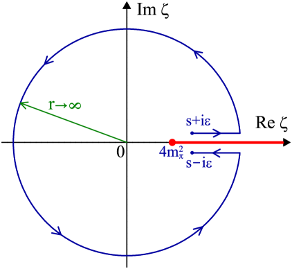
Figure 1: The integration contour in Eq. (4). The physical cut $\zeta\geq 4m_{\pi}^{2}$ of the Adler function $D(-\zeta)$ (3) is shown along the positive semiaxis of real $\zeta$.

In the ultraviolet asymptotic $s\to\infty$ the effects due to the masses of the involved particles can be safely neglected, so that in Eq. (4) one can employ the perturbative approximation of the Adler function [31]

$$D^{(\ell)}_{{\rm pert}}(Q^{2})=1+\sum_{j=1}^{\ell}d_{j}\left[a^{\mbox{\scriptsize$(\ell)$}}_{\mbox{\scriptsize s}}(Q^{2})\right]^{j}$$ (5)

(the common prefactor $N_{\mbox{\scriptsize c}}\sum_{f=1}^{n_{\mbox{\tiny f}}}Q_{f}^{2}$ is omitted throughout, where $N_{\mbox{\scriptsize c}}=3$ stands for the number of colors, $Q_{f}$ denotes the electric charge of $f$–th quark, and $n_{\mbox{\scriptsize f}}$ is the number of active flavors). In Eq. (5) $d_{j}$ stand for the relevant perturbative coefficients ($d_{1}=4/\beta_{0}$, $\beta_{0}=11-2n_{\mbox{\scriptsize f}}/3$), whereas $a^{\mbox{\scriptsize$(\ell)$}}_{\mbox{\scriptsize s}}(Q^{2})$ is the $\ell$–loop perturbative QCD couplant $a^{\mbox{\scriptsize$(\ell)$}}_{\mbox{\scriptsize s}}(Q^{2})=\alpha^{\mbox{\scriptsize$(\ell)$}}_{\mbox{\scriptsize s}}(Q^{2})\,\beta_{0}/(4\pi)$, which satisfies the renormalization group equation ($B_{j}=\beta_{j}/\beta^{j+1}_{0}$)

$$\frac{d\,\ln\bigl{[}a^{\mbox{\scriptsize$(\ell)$}}_{\mbox{\scriptsize s}}(\mu^{2})\bigr{]}}{d\,\ln\mu^{2}}=-\sum_{j=0}^{\ell-1}B_{j}\left[a^{\mbox{\scriptsize$(\ell)$}}_{\mbox{\scriptsize s}}(\mu^{2})\right]^{j+1}.$$ (6)

The use of the perturbative approximation of the Adler function (5) in Eq. (4) casts the latter to (see Ref. [13])

$$R^{(\ell)}(s)=1+\int\limits_{s}^{\infty}\!\rho^{(\ell)}_{{\rm pert}}(\sigma)\,\frac{d\sigma}{\sigma},$$ (7)

where

$$\rho^{(\ell)}_{{\rm pert}}(\sigma)\!=\!\frac{1}{2\pi i}\!\lim_{\varepsilon\to 0_{+}}\Bigl{[}d^{(\ell)}_{{\rm pert}}(-\sigma-i\varepsilon)-d^{(\ell)}_{{\rm pert}}(-\sigma+i\varepsilon)\!\Bigr{]}\;\,$$ (8)

denotes the $\ell$–loop perturbative spectral function, with $d^{(\ell)}_{{\rm pert}}(Q^{2})$ being the strong correction to the Adler function (5).

To properly account for the effects due to continuation of the spacelike perturbative results into the timelike domain one first has to calculate the spectral function (8) and then perform (explicitly or numerically) the integration (7). It is worth noting that the form of the resulting expression for the function $R(s)$ drastically differs from that of the perturbative power series (5). For example, at the one–loop level Eq. (7) reads (see papers [35, 27, 36, 13])

$$R^{(1)}(s)=1+d_{1}\!\left\{\frac{1}{2}-\frac{1}{\pi}\arctan\!\left[\frac{\ln(s/\Lambda^{2})}{\pi}\right]\right\}\!,$$ (9)

where $\Lambda$ is the QCD scale parameter and it is assumed that $\arctan(x)$ is a monotone nondecreasing function of its argument. At the same time, it appears that the re–expansion of Eq. (7) in the ultraviolet asymptotic $s\to\infty$ leads to an approximate expression for the function $R(s)$, which resembles Eq. (5).

In particular, at high energies the $\ell$–loop strong correction to the $R$–ratio (7) can be represented as

$$r^{(\ell)}(s)=\int\limits_{\ln w}^{\infty}\!\rho^{(\ell)}_{y}(y)\,dy,\qquad y=\ln\left(\frac{\sigma}{\Lambda^{2}}\right)\!,$$ (10)

where $w=s/\Lambda^{2}$,

$$\rho^{(\ell)}_{y}(y)=\frac{1}{2\pi i}\,\Bigl{[}d^{(\ell)}_{y}(y-i\pi)-d^{(\ell)}_{y}(y+i\pi)\Bigr{]},$$ (11)

and $d^{(\ell)}_{y}(y)=d^{(\ell)}_{{\rm pert}}\bigl{[}\exp(y)\Lambda^{2}\bigr{]}$. Applying the Taylor expansion to Eq. (11) one arrives at

$$r^{(\ell)}_{{\rm pert}}(s)\!\!\!\! = \!\!\!\!d^{(\ell)}_{{\rm pert}}(|s|)+$$ (12)

$$+ \!\!\!\!\left.\sum_{n=1}^{\infty}\frac{(-1)^{n}\pi^{2n}}{(2n+1)!}\frac{d^{2n}}{dy^{2n}}\,d^{(\ell)}_{y}(y)\right|_{y=\ln w}.$$

The right–hand side of this equation constitutes the sum of the naive continuation ($Q^{2}\to|s|$) of the strong correction to the Adler function into the timelike domain (first line) and an infinite number of the so–called $\pi^{2}$–terms (second line). Note that Eq. (12) is only valid for $\sqrt{s}>\exp(\pi/2)\Lambda$.

The strong correction to the Adler function entering Eq. (12) reads

$$d^{(\ell)}_{y}(y)=\sum_{j=1}^{\ell}d_{j}\left[a^{(\ell)}_{y}(y)\right]^{j}\!,$$ (13)

where $a^{(\ell)}_{y}(y)=a^{\mbox{\scriptsize$(\ell)$}}_{\mbox{\scriptsize s}}\bigl{[}\exp(y)\Lambda^{2}\bigr{]}$. In turn, Eq. (6) implies

$$\frac{d^{n}}{dy^{n}}\,\left[a^{(\ell)}_{y}(y)\right]^{j}\!\!\!\! = \!\!\!\!(-1)^{n}\times$$ (14)

$$\!\!\!\!\times\sum_{k_{1}=0}^{\ell-1}\ldots\sum_{k_{n}=0}^{\ell-1}\,\prod_{t=0}^{n-1}\Bigl{(}j+t+k_{1}+\ldots+k_{t}\Bigr{)}\times$$

$$\!\!\!\!\times\prod_{p=1}^{n}B_{k_{p}}\left[a^{(\ell)}_{y}(y)\right]^{j+n+k_{1}+\ldots+k_{n}}\!,$$

that eventually leads to the following expression for the $\ell$–loop perturbative approximation of $R$–ratio of electron–positron annihilation into hadrons:

$$R^{(\ell)}_{{\rm pert}}(s)\!\!\!\! = \!\!\!\!1+\sum_{j=1}^{\ell}d_{j}\left[a^{(\ell)}_{{\rm s}}(|s|)\right]^{j}-$$ (15)

$$\!\!\!\!-\sum_{j=1}^{\ell}d_{j}\sum_{n=1}^{\infty}\frac{(-1)^{n+1}\pi^{2n}}{(2n+1)!}\sum_{k_{1}=0}^{\ell-1}\ldots\sum_{k_{2n}=0}^{\ell-1}\,\prod_{p=1}^{2n}B_{k_{p}}\times$$

$$\!\!\!\!\times\!\prod_{t=0}^{2n-1}\Bigl{(}j+t+k_{1}+\ldots+k_{t}\Bigr{)}\!\left[a^{(\ell)}_{{\rm s}}(|s|)\right]^{j+2n+k_{1}+\ldots+k_{2n}}\!\!.\quad$$

In particular, this equation testifies that at any given loop level the re–expansion of the $R$–ratio (7) at high energies can be cast to the form of power series in the naive continuation of the strong running coupling into the timelike domain. Additionally, Eq. (15) explicitly demonstrates that the $\pi^{2}$–terms appear starting from the three–loop level only.

Commonly, on the right–hand side of Eq. (15) one discards the $\pi^{2}$–terms of the orders higher than the loop level on hand, that results in

$$R^{(\ell)}_{{\rm pert}}(s)\simeq 1+\!\sum_{j=1}^{\ell}r_{j}\left[a^{\mbox{\scriptsize$(\ell)$}}_{\mbox{\scriptsize s}}(|s|)\right]^{j}\!,\quad r_{j}=d_{j}-\delta_{j}.$$ (16)

It is necessary to emphasize here that Eqs. (15) and (16) are only valid for $\sqrt{s}>\exp(\pi/2)\Lambda\simeq 4.81\,\Lambda$, so that the lower boundary of the convergence range of the re–expanded $R$–ratio (16) may be as high as $(1.5\ldots 2.0)\,$GeV for $\Lambda\simeq(300\ldots 400)\,$MeV. This issue is illustrated by Fig. 2, which displays the one–loop function $R^{(1)}(s)$ (9) (solid curve), its re–expansion

$$R^{(1)}(s)\!\!\!\! \simeq \!\!\!\!1+d_{1}\biggl{[}a^{\mbox{\scriptsize$(1)$}}_{\mbox{\scriptsize s}}(|s|)-\frac{\pi^{2}}{3}\frac{1}{\ln^{3}w}+\frac{\pi^{4}}{5}\frac{1}{\ln^{5}w}-$$ (17)

$$- \!\!\!\!\frac{\pi^{6}}{7}\frac{1}{\ln^{7}w}+\mathcal{O}\left(\frac{1}{\ln^{9}w}\right)\biggr{]},\quad\;s\to\infty$$

truncated at various orders (dashed curves), and the lower boundary of the convergence range of Eq. (17) (vertical line). In Eq. (17) $a^{\mbox{\scriptsize$(1)$}}_{\mbox{\scriptsize s}}(Q^{2})=1/\ln z$ stands for the one–loop perturbative couplant, $z=Q^{2}/\Lambda^{2}$, and $w=s/\Lambda^{2}$. In particular, Fig. 2 shows Eq. (17) truncated at the order $\ln^{-1}z$, which corresponds to the naive continuation of the one–loop perturbative approximation of the Adler function (5) into the timelike domain $D^{(1)}_{{\rm pert}}(|s|)$ (label “a”), at the order $\ln^{-7}z$ (label “b”), and at the order $\ln^{-25}z$ (label “c”). As one can infer from this Figure, the truncation of Eq. (17) at first order (that results in the one–loop expression (16) with $\delta_{1}=0$) turns out to be a rather rough approximation. Specifically, the relative difference between the one–loop strong correction (16), which basically discards all the $\pi^{2}$–terms, and the one–loop strong correction (9), which, on the contrary, incorporates the $\pi^{2}$–terms to all orders, appears to be about $20\,\%$ at $\sqrt{s}=2.5\,$GeV for $n_{\mbox{\scriptsize f}}=3$ active flavors and $\Lambda=350\,$MeV.

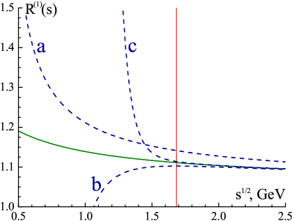
Figure 2: The one–loop function $R^{(1)}(s)$ (9) (solid curve) and its re–expansion (17) (dashed curves) truncated at the orders $\ln^{-1}z$ (curve “a”), $\ln^{-7}z$ (curve “b”), and $\ln^{-25}z$ (curve “c”). Vertical line marks the lower boundary of the convergence range of the re–expansion (17). The values of parameters: $n_{\mbox{\tiny f}}=3$ active flavors, $\Lambda=350\,$MeV.

In the perturbative approximation of the $R$–ratio (16) the coefficients $\delta_{j}$, which embody the corresponding $\pi^{2}$–terms, have been calculated up to the sixth order in papers [37, 38], namely

$$\delta_{1}=0,$$ (18)

$$\delta_{2}=0,$$ (19)

$$\delta_{3}=\frac{\pi^{2}}{3}d_{1},$$ (20)

$$\delta_{4}=\frac{\pi^{2}}{3}\left(\frac{5}{2}d_{1}B_{1}+3d_{2}\right)\!,$$ (21)

$$\delta_{5}\!\!\!\! = \!\!\!\!\frac{\pi^{2}}{3}\left[\frac{3}{2}d_{1}\left(B_{1}^{2}+2B_{2}\right)+7d_{2}B_{1}+6d_{3}\right]-$$ (22)

$$- \!\!\!\!\frac{\pi^{4}}{5}d_{1},$$

$$\delta_{6}\!\!\!\! = \!\!\!\!\frac{\pi^{2}}{3}\biggl{[}\frac{7}{2}d_{1}\left(B_{1}B_{2}+B_{3}\right)+4d_{2}\left(B_{1}^{2}+2B_{2}\right)+$$ (23)

$$+ \!\!\!\!\frac{27}{2}d_{3}B_{1}+10d_{4}\biggr{]}-\frac{\pi^{4}}{5}\left(\frac{77}{12}d_{1}B_{1}+5d_{2}\right)\!.$$

The higher–order coefficients $\delta_{j}$ (16) read

$$\delta_{7}\!\!\!\! = \!\!\!\!\frac{\pi^{2}}{3}\biggl{[}4d_{1}\left(B_{1}B_{3}+\frac{1}{2}B_{2}^{2}+B_{4}\right)+$$ (24)

$$+ \!\!\!\!9d_{2}\left(B_{1}B_{2}+B_{3}\right)+\frac{15}{2}d_{3}\left(B_{1}^{2}+2B_{2}\right)+$$

$$+ \!\!\!\!22d_{4}B_{1}+15d_{5}\biggr{]}-\frac{\pi^{4}}{5}\biggl{[}\frac{5}{6}d_{1}\left(17B_{1}^{2}+12B_{2}\right)+$$

$$+ \!\!\!\!\frac{57}{2}d_{2}B_{1}+15d_{3}\biggr{]}+\frac{\pi^{6}}{7}d_{1},$$

$$\delta_{8}\!\!\!\! = \!\!\!\!\frac{\pi^{2}}{3}\biggl{[}\frac{9}{2}d_{1}\left(B_{1}B_{4}+B_{2}B_{3}+B_{5}\right)+$$ (25)

$$+ \!\!\!\!10d_{2}\left(\!B_{1}B_{3}+\!\frac{B_{2}^{2}}{2}\!+B_{4}\!\right)+\!\frac{33}{2}d_{3}\left(B_{1}B_{2}+\!B_{3}\right)+$$

$$+ \!\!\!\!12d_{4}\left(B_{1}^{2}+2B_{2}\right)+\frac{65}{2}d_{5}B_{1}+21d_{6}\biggr{]}-$$

$$- \!\!\!\!\frac{\pi^{4}}{5}\biggl{[}\frac{15}{8}d_{1}\left(7B_{1}^{3}+22B_{1}B_{2}+8B_{3}\right)+$$

$$+ \!\!\!\!\frac{5}{12}d_{2}\left(139B_{1}^{2}+96B_{2}\right)\!+\!\frac{319}{4}d_{3}B_{1}+35d_{4}\!\biggr{]}\!+$$

$$+ \!\!\!\!\frac{\pi^{6}}{7}\left(\frac{223}{20}d_{1}B_{1}+7d_{2}\right)\!.$$

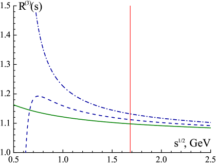
Figure 3: Three–loop function $R^{(3)}(s)$ (Eq. (7), solid curve), its perturbative approximation $R^{(3)}_{{\rm pert}}(s)$ (Eq. (16), dashed curve), and the naive continuation of the three–loop Adler function into the timelike domain $D^{(3)}_{{\rm pert}}(|s|)$ (Eq. (5), dot–dashed curve). Vertical line marks the lower boundary of the convergence range of the perturbative approximation of $R$–ratio (16). The values of parameters: $n_{\mbox{\tiny f}}=3$ active flavors, $\Lambda=350\,$MeV.

It appears that the values of the coefficients $\delta_{j}$ ($j\geq 3$) substantially exceed the values of the corresponding perturbative coefficients $d_{j}$, that drastically affects the perturbative approximation of $R$–ratio (16). For example, for $n_{\mbox{\scriptsize f}}=3$ active flavors $d_{3}=0.559$, whereas $\delta_{3}=1.462$, so that the third–order term in Eq. (16) turns out to be amplified and even sign–reversed ($r_{3}=-0.903$). This issue is illustrated by Fig. 3, which displays the three–loop function $R^{(3)}(s)$ (Eq. (7), solid curve), which includes the $\pi^{2}$–terms to all orders, its perturbative approximation $R^{(3)}_{{\rm pert}}(s)$ (Eq. (16), dashed curve), which retains only the first non–vanishing $\pi^{2}$–term (20), and the naive continuation of the three–loop Adler function into the timelike domain $D^{(3)}_{{\rm pert}}(|s|)$ (Eq. (5), dot–dashed curve), which discards all the $\pi^{2}$–terms. The lower boundary of the convergence range of the perturbative approximation of $R$–ratio (16) at $\sqrt{s}=\exp(\pi/2)\Lambda$ is shown in Fig. 3 by vertical line. It is worth noting also that for $n_{\mbox{\scriptsize f}}=3$ active flavors and $\Lambda=350\,$MeV the relative difference between the strong corrections $d^{(3)}_{{\rm pert}}(|s|)$ (5) and $r^{(3)}(s)$ (7) at $\sqrt{s}=2.5\,$GeV exceeds $20\,\%$, whereas the relative difference between the strong corrections $r^{(3)}_{{\rm pert}}(s)$ (16) and $r^{(3)}(s)$ (7) turns out to be about $10\,\%$.

An evident advantage of the representation of the $R$–ratio of electron–positron annihilation into hadrons in the form of Eq. (7) is that the latter properly accounts for the effects due to continuation of the spacelike perturbative results into the timelike domain and embodies (or “resummates”) the $\pi^{2}$–terms to all orders. The integration in Eq. (7) can easily be performed in the way described in papers [32, 33].

References

- [1] H.M. Fried, Y. Gabellini, T. Grandou, and Y.-M. Sheu, Eur. Phys. J. C 65, 395 (2010); Annals Phys. 338, 107 (2013); H.M. Fried, T. Grandou, and Y.-M. Sheu, ibid. 344, 78 (2014); H.M. Fried, P.H. Tsang, Y. Gabellini, T. Grandou, and Y.-M. Sheu, ibid. 359, 1 (2015).
- [2] Y. Kim, I.J. Shin, and T. Tsukioka, Prog. Part. Nucl. Phys. 68, 55 (2013); S.J. Brodsky, G.F. de Teramond, H.G. Dosch, and J. Erlich, Phys. Rept. 584, 1 (2015).
- [3] V.A. Novikov, M.A. Shifman, A.I. Vainshtein, and V.I. Zakharov, Nucl. Phys. B 174, 378 (1980); Fortsch. Phys. 32, 585 (1984); E. de Rafael, arXiv:hep-ph/9802448; P. Colangelo and A. Khodjamirian, arXiv:hep-ph/0010175; S. Narison, World Sci. Lect. Notes Phys. 26, 1 (1989); Nucl. Phys. B (Proc. Suppl.) 164, 225 (2007); Nucl. Phys. B (Proc. Suppl.) 207, 315 (2010); Nucl. Part. Phys. Proc. 258, 189 (2015).
- [4] G.S. Bali, Phys. Rept. 343, 1 (2001); P. Hagler, ibid. 490, 49 (2010); E. Shintani et al. [JLQCD and TWQCD Collaborations], Phys. Rev. D 79, 074510 (2009); P. Boyle, L. Del Debbio, E. Kerrane, and J. Zanotti, ibid. 85, 074504 (2012); A. Francis, B. Jager, H.B. Meyer, and H. Wittig, ibid. 88, 054502 (2013); S. Aoki et al. [FLAG Working Group], arXiv:1607.00299 [hep-lat].
- [5] A.E. Dorokhov and W. Broniowski, Eur. Phys. J. C 32, 79 (2003); A.E. Dorokhov, Phys. Rev. D 70, 094011 (2004); Nucl. Phys. A 790, 481 (2007); A.E. Dorokhov, A.E. Radzhabov, and A.S. Zhevlakov, Eur. Phys. J. C 71, 1702 (2011); 72, 2227 (2012); 75, 417 (2015); JETP Lett. 100, 133 (2014); arXiv:1608.02331 [hep-ph].
- [6] M. Frasca, Phys. Rev. C 84, 055208 (2011); JHEP 1311, 099 (2013); Eur. Phys. J. Plus 131, 199 (2016); arXiv:1509.05292 [math-ph].
- [7] A.V. Nesterenko and J. Papavassiliou, J. Phys. G 32, 1025 (2006).
- [8] A.V. Nesterenko, Phys. Rev. D 88, 056009 (2013); J. Phys. G 42, 085004 (2015).
- [9] F. Guerrero and A. Pich, Phys. Lett. B 412, 382 (1997); A. Pich and J. Portoles, Phys. Rev. D 63, 093005 (2001); V. Bernard and E. Passemar, Phys. Lett. B 661, 95 (2008).
- [10] R. Garcia–Martin, R. Kaminski, J.R. Pelaez, and J. Ruiz de Elvira, Phys. Rev. Lett. 107, 072001 (2011); R. Garcia–Martin, R. Kaminski, J.R. Pelaez, J. Ruiz de Elvira, and F.J. Yndurain, Phys. Rev. D 83, 074004 (2011).
- [11] G. Colangelo, M. Hoferichter, M. Procura, and P. Stoffer, JHEP 1509, 074 (2015).
- [12] D.V. Shirkov and I.L. Solovtsov, Phys. Rev. Lett. 79, 1209 (1997); Theor. Math. Phys. 150, 132 (2007).
- [13] K.A. Milton and I.L. Solovtsov, Phys. Rev. D 55, 5295 (1997); 59, 107701 (1999).
- [14] G. Cvetic and C. Valenzuela, Braz. J. Phys. 38, 371 (2008); G. Cvetic and A.V. Kotikov, J. Phys. G 39, 065005 (2012); A.P. Bakulev, Phys. Part. Nucl. 40, 715 (2009); N.G. Stefanis, ibid. 44, 494 (2013).
- [15] G. Cvetic, A.Y. Illarionov, B.A. Kniehl, and A.V. Kotikov, Phys. Lett. B 679, 350 (2009); A.V. Kotikov, PoS (Baldin ISHEPP XXI), 033 (2013); A.V. Kotikov and B.G. Shaikhatdenov, Phys. Part. Nucl. 44, 543 (2013); Phys. Atom. Nucl. 78, 525 (2015); A.V. Kotikov, V.G. Krivokhizhin, and B.G. Shaikhatdenov, J. Phys. G 42, 095004 (2015).
- [16] C. Contreras, G. Cvetic, O. Espinosa, and H.E. Martinez, Phys. Rev. D 82, 074005 (2010); C. Ayala, C. Contreras, and G. Cvetic, ibid. 85, 114043 (2012); G. Cvetic and C. Villavicencio, ibid. 86, 116001 (2012); C. Ayala and G. Cvetic, ibid. 87, 054008 (2013); P. Allendes, C. Ayala, and G. Cvetic, ibid. 89, 054016 (2014).
- [17] M. Baldicchi and G.M. Prosperi, Phys. Rev. D 66, 074008 (2002); AIP Conf. Proc. 756, 152 (2005); M. Baldicchi, G.M. Prosperi, and C. Simolo, ibid. 892, 340 (2007); M. Baldicchi, A.V. Nesterenko, G.M. Prosperi, D.V. Shirkov, and C. Simolo, Phys. Rev. Lett. 99, 242001 (2007); M. Baldicchi, A.V. Nesterenko, G.M. Prosperi, and C. Simolo, Phys. Rev. D 77, 034013 (2008).
- [18] A.C. Aguilar, A.V. Nesterenko, and J. Papavassiliou, J. Phys. G 31, 997 (2005); Nucl. Phys. B (Proc. Suppl.) 164, 300 (2007).
- [19] A.V. Nesterenko, Phys. Rev. D 62, 094028 (2000); 64, 116009 (2001); N. Christiansen, M. Haas, J.M. Pawlowski, and N. Strodthoff, Phys. Rev. Lett. 115, 112002 (2015); N. Mueller and J.M. Pawlowski, Phys. Rev. D 91, 116010 (2015); R. Lang, N. Kaiser, and W. Weise, Eur. Phys. J. A 51, 127 (2015).
- [20] K.A. Milton, I.L. Solovtsov, and O.P. Solovtsova, Phys. Lett. B 439, 421 (1998); Phys. Rev. D 60, 016001 (1999); R.S. Pasechnik, D.V. Shirkov, and O.V. Teryaev, ibid. 78, 071902 (2008); R.S. Pasechnik, J. Soffer, and O.V. Teryaev, ibid. 82, 076007 (2010).
- [21] K.A. Milton, I.L. Solovtsov, and O.P. Solovtsova, Phys. Lett. B 415, 104 (1997); K.A. Milton, I.L. Solovtsov, O.P. Solovtsova, and V.I. Yasnov, Eur. Phys. J. C 14, 495 (2000).
- [22] G. Ganbold, Phys. Rev. D 79, 034034 (2009); 81, 094008 (2010); PoS (Confinement X), 065 (2013).
- [23] A. Bakulev, K. Passek–Kumericki, W. Schroers, and N. Stefanis, Phys. Rev. D 70, 033014 (2004); 70, 079906(E) (2004); A. Bakulev, A. Pimikov, and N. Stefanis, ibid. 79, 093010 (2009); N. Stefanis, Nucl. Phys. B (Proc. Suppl.) 152, 245 (2006).
- [24] G. Cvetic, R. Kogerler, and C. Valenzuela, Phys. Rev. D 82, 114004 (2010); J. Phys. G 37, 075001 (2010); G. Cvetic and R. Kogerler, Phys. Rev. D 84, 056005 (2011).
- [25] O. Teryaev, Nucl. Phys. B (Proc. Suppl.) 245, 195 (2013); A.V. Sidorov and O.P. Solovtsova, Nonlin. Phenom. Complex Syst. 16, 397 (2013); Mod. Phys. Lett. A 29, 1450194 (2014).
- [26] S.L. Adler, Phys. Rev. D 10, 3714 (1974).
- [27] A.V. Radyushkin, report JINR E2–82–159 (1982); JINR Rapid Commun. 78, 96 (1996); arXiv:hep-ph/9907228.
- [28] N.V. Krasnikov and A.A. Pivovarov, Phys. Lett. B 116, 168 (1982).
- [29] A.V. Nesterenko and J. Papavassiliou, Phys. Rev. D 71, 016009 (2005); Int. J. Mod. Phys. A 20, 4622 (2005); Nucl. Phys. B (Proc. Suppl.) 152, 47 (2005); 164, 304 (2007).
- [30] A.V. Nesterenko, Nucl. Phys. B (Proc. Suppl.) 186, 207 (2009); arXiv:1110.3415 [hep-ph]; Nucl. Part. Phys. Proc. 258, 177 (2015); AIP Conf. Proc. 1701, 040016 (2016).
- [31] P.A. Baikov, K.G. Chetyrkin, and J.H. Kuhn, Phys. Rev. Lett. 101, 012002 (2008); 104, 132004 (2010); P.A. Baikov, K.G. Chetyrkin, J.H. Kuhn, and J. Rittinger, Phys. Lett. B 714, 62 (2012).
- [32] A.V. Nesterenko, Int. J. Mod. Phys. A 18, 5475 (2003).
- [33] A.V. Nesterenko and C. Simolo, Comput. Phys. Commun. 181, 1769 (2010); 182, 2303 (2011).
- [34] A.P. Bakulev and V.L. Khandramai, Comput. Phys. Commun. 184, 183 (2013); C. Ayala and G. Cvetic, ibid. 190, 182 (2015); 199, 114 (2016).
- [35] B. Schrempp and F. Schrempp, Z. Phys. C 6, 7 (1980).
- [36] A.A. Pivovarov, Nuovo Cim. A 105, 813 (1992).
- [37] J.D. Bjorken, report SLAC–PUB–5103 (1989).
- [38] A.L. Kataev and V.V. Starshenko, Mod. Phys. Lett. A 10, 235 (1995).