Heralded quantum controlled phase gates with dissipative
dynamics in macroscopically-distant resonators

Abstract

Heralded near-deterministic multi-qubit controlled phase gates with integrated error detection have recently been proposed by Borregaard et al. [Phys. Rev. Lett. 114, 110502 (2015)]. This protocol is based on a single four-level atom (a heralding quartit) and $N$ three-level atoms (operational qutrits) coupled to a single-resonator mode acting as a cavity bus. Here we generalize this method for two distant resonators without the cavity bus between the heralding and operational atoms. Specifically, we analyze the two-qubit controlled-Z gate and its multi-qubit-controlled generalization (i.e., a Toffoli-like gate) acting on the two-lowest levels of $N$ qutrits inside one resonator, with their successful actions being heralded by an auxiliary microwave-driven quartit inside the other resonator. Moreover, we propose a circuit-quantum-electrodynamics realization of the protocol with flux and phase qudits in linearly-coupled transmission-line resonators with dissipation. These methods offer a quadratic fidelity improvement compared to cavity-assisted deterministic gates.

I introduction

The ability to carry out quantum gates is one of the central requirements for a functional quantum computer Nielsen and Chuang (2010). For this reason, quantum gates have been extensively studied in theoretical and experimental in various systems. These include (for reviews see Buluta et al. (2011); Xiang et al. (2013) and references therein): superconducting circuits, trapped ions, diamond nitrogen-vacancy centers, semiconductor nanostructures, or linear-optical setups. Despite of such substantial efforts, the environment-induced decoherence still represents a major hurdle in the quest for perfect quantum gates. To protect quantum systems from decoherence, three basic approaches have been explored; namely, quantum error correction, dynamical decoupling, and decoherence-free subspaces (for reviews see Lid ; Devitt et al. (2013) and references therein). Such approaches try to cope with decoherence, and thus, to prevent the leakage of quantum information from a quantum system into its environment.

Alternatively, there exists a very distinct way, where decoherence acts as a resource, rather than as a traditional noise source Bose et al. (1999); Chimczak et al. (2005); Kraus et al. (2008); Verstraete et al. (2009); Krauter et al. (2011). Recent progress in treating open quantum systems has yielded an effective operator formalism Kastoryano et al. (2011); Reiter and Sørensen (2012). As in Ref. Reiter and Sørensen (2012), (i) when the interactions between the ground- and excited-state subspaces of an open system initially in its ground state are sufficiently weak (so it can be considered as perturbations of the two subspaces) and also (ii) when the interactions inside the ground-state subspace are much smaller than those inside the excited-state subspace, one can adiabatically eliminate these excited states in the presence of both unitary and dissipative dynamics, and obtain an effective master equation containing the effective Hamiltonian, as well as the effective Lindblad operators, associated only with the ground states. In addition to reducing the complexity of the time evolution for an open quantum system, this approximation treatment is applicable to the explorations of decay processes, hence may lead to a better performance than that in the case of relying upon coherent-unitary dynamics.

So far, such a formalism has been widely used for dissipative entanglement preparation Kastoryano et al. (2011); Shen et al. (2011); Reiter et al. (2012); Lin et al. (2013); Sweke et al. (2013); Reiter et al. (2013); Su et al. (2014), quantum phase estimation Davis et al. (2016) and other applications Schönleber et al. (2015); Schempp et al. (2015); Dooley et al. (2016); Ramos et al. (2016). In particular, Borregaard et al. presented a heralded near-deterministic method for quantum gates in a single optical cavity Borregaard et al. (2015), with a significant improvement in the error scaling, compared to deterministic cavity-based gates. However, in order to carry out scalable quantum information processing, a distant herald for quantum gates in coupled resonators is of a great importance concerning both experimental feasibility and fundamental tests of quantum mechanics.

The goal of this paper is to propose and analyze an approach to heralding controlled quantum gates in two macroscopically distant resonators, by generalizing the single-resonator method of Borregaard et al. Borregaard et al. (2015). We use an auxiliary quartit atom, which is located in one resonator and driven by two coherent fields, to distantly herald controlled phase gates acting on the two lowest levels of qutrit atoms, which are located in the other resonator. These controlled phase operations studied here include the two-qubit controlled-Z gate (controlled-sign gate) and its multi-qubit-controlled version referred to as a Toffoli-like gate. We also propose a realization of these gates using superconducting artificial atoms in a dissipative circuit quantum electrodynamics (QED) system.

Circuit-QED systems, which are composed of superconducting artificial atoms coupled to superconducting resonators, offer promising platforms for quantum engineering and quantum-information processing You and Nori (2005); Clarke and Wilhelm (2008); DiCarlo et al. (2010); Buluta et al. (2011); Lucero et al. (2012); Georgescu et al. (2014). Although artificial and natural atoms are similar in various properties including, for example, discrete anharmonic energy levels You and Nori (2003); Blais et al. (2004); You and Nori (2011), superconducting atoms have some substantial advantages over natural atoms. These include: (i) The spacing between energy levels, decoherence rates, and coupling strengths between different circuit elements are tunable by adjusting external parameters, thus, providing flexibility for quantum information processing Buluta et al. (2011); Xiang et al. (2013); (ii) The potential energies of natural atoms have an inversion symmetry, leading to a well-defined parity symmetry for each eigenstate. Thus, an allowable dipole transition requires a parity change, and can only occur between the two eigenstates having different parities. However, the potential energies of superconducting artificial atoms can be controlled Liu et al. (2005) by external parameters and, in turn, the inversion symmetry can be broken or unbroken. When the symmetry is unbroken, each eigenstate of an artificial atom can have a well-defined parity symmetry and, thus, exhibit a transition behavior similar to natural atoms. But when the symmetry is broken then there is no well-defined parity symmetry for each eigenstate and, thus, the microwave-induced single-photon transition between any two eigenstates can be possible. That is, the selection rules can easily be modified Deppe et al. (2008); (iii) The couplings between different circuit elements can be strong, ultrastrong (for reviews see You and Nori (2011); Xiang et al. (2013)), or even deep strong Yoshihara et al. (2017), which, in particular, enable efficient state preparation within a short time and with a high fidelity.

Specifically, based on circuit QED we realize a distant herald for a multi-qubit Toffoli-like gate, whose the fidelity scaling is quadratically improved as compared to unitary-dynamics-based gates in cavities Borregaard et al. (2015); Sørensen and Mølmer (2003); moreover, heralded controlled-Z gates even with more significant improvements can also be achieved by using single-qubit operations. Note that the conditional measurement on the heralding atom is performed to remove the detected errors from the quantum gate. Thus, these detected errors can only reduce the success probability but not the gate fidelity. When the gate is successful, the gate fidelity can still be very high as limited only by the undetected errors. In contrast to previous works, a macroscopically distant herald for quantum gates is proposed in superconducting circuits via the combined effect of the dissipative and unitary dynamics, thereby having the potential advantage of high efficiency in experimental scenarios. By considering only the $d$ lowest energy levels of a superconducting artificial atom, one can use them as a logical qudit for performing quantum operations. In special cases, one can operate with a qubit (for $d=2$), qutrit (for $d=3$), or quartit (ququart, for $d=4$). Here we will analyze these special qudits.

This paper is organized as follows. In Sec. II, we describe a physical model for heralded quantum phase gates and propose a superconducting circuit for its realization. In Sec. III, we derive the effective master equation which is used in Sec. IV to realize a multi-qubit Toffoli-like gate. Working with single-qubit operations, Sec. V then presents a heralded controlled-Z gate. The last section is our summary. A detailed derivation of the effective master equation, which is applied in Sec. III, is given in the Appendix.

II Physical model in superconducting circuits

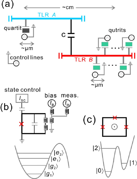
Figure 1: (Color online) (a) Schematic diagram of a superconducting circuit layout, which shows our implementation of a heralded near-deterministic controlled multi-qubit Toffoli-like gate and, in a special case, the two-qubit controlled-Z (CZ) gate. Two transmission-line resonators (TLRs), labeled by $A$ and $B$, are linearly coupled via a capacitor. Resonator $A$ is coupled to a phase quartit (e.g., a four-level qudit) via a capacitance, while resonator $B$ is coupled to $N$ identical flux qutrits (e.g., three-level qudits). Such circuit elements can be controlled via ac and dc signals through the control lines. The distance between the qudit and qutrits can be of order of cm due to the macroscopic length of the resonators. Panel (b) shows an energy-level diagram for a prototypical phase quartit, while panel (c) depicts that diagram for a typical flux qutrit. Here we assume that the energy potential for the quartit is cubic and for the qutrit is an asymmetric double well. Note that both flux and phase qudits can be tuned (for example, by adjusting the flux bias in the qudit loop) to obtain exactly two, three, or four levels. For example, following the method of Refs. Martinis et al. (2002); Neeley et al. (2009), the phase qudit state can be controlled by an ac signal $I_{\rm SC}$, while a dc signal $I_{\rm B}$ is used to bias the circuit. Moreover, a short measurement pulse $I_{\rm M}$ is applied to decrease the barrier in the energy potential well of panel (b) to enable given upper states to tunnel out of the well. These tunneling currents can be detected by another SQUID which, for brevity, is not plotted here. Thus, the proposed quantum gates can be realized, based solely on flux or phase qudits, or other superconducting qudits. The successful operation of this Toffoli-like gate is heralded by the detection of the quartit in its ground state $|g_{1}\rangle$.

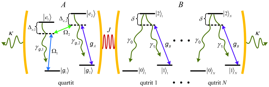
Figure 2: (Color online) Energy-level diagram showing allowed transitions and couplings in the circuit-QED system depicted in Fig. 1. Two single-mode resonators, labeled by $A$ and $B$ are coupled with a strength $J$. An auxiliary, quartit atom, which acts as a heralding device, is confined in the resonator $A$. Two microwave fields drive off-resonantly the transitions $|g_{1}\rangle\rightarrow|e_{1}\rangle$ and $|e_{1}\rangle\rightarrow|e_{2}\rangle$ of the auxiliary quartit, with strengths $\Omega_{1}$ and $\Omega_{2}$, respectively. Moreover, the states $|g_{2}\rangle$ and $|e_{2}\rangle$ are coupled by the resonator mode $a_{A}$ with strength $g_{A}$. In the resonator $B$, there are confined $N$ qutrit atoms, for which the two lowest-energy levels can be treated as qubits. For each qutrit atom, only the state $|1\rangle$ is coupled to $|2\rangle$ by the resonator mode $a_{B}$ with strength $g_{B}$. Upon restricting our discussion to sufficiently weak microwave drive $\Omega_{1}$, we could adiabatically eliminate the excited states of the total system to yield an effective Lindblad-type master equation, which involves the ground states only. The resulting dynamics allows for the realization of the controlled-phase gates, which can successfully occur if the auxiliary quartit in the state $|g_{1}\rangle$ is measured.

Table 1: Basic notations used in this paper. Here, $x=1,2$ and $z=0,1,2$.

notation	Meaning
$\omega_{g\left(e\right),x}$	$|g_{x}\rangle$-($|e_{x}\rangle$-) level frequency
$\omega_{z}$	$|z\rangle$-level frequency
$\omega_{c}$	Common resonance frequency of resonators $A$ and $B$
$\omega_{m,x}$	Microwave drive $x$ frequency
$\Omega_{x}$	Microwave $x$ driving amplitude strength
$g_{A}$ ($g_{B}$)	Coupling strength between the quartit (qutrit) atom and resonator $A$ ($B$)
$J$	Inter-resonator coupling strength
$\gamma_{g,x}$	Decay rate from level $|e_{x}\rangle$ to $|g_{x}\rangle$
$\gamma_{x-1}$	Decay rate from level $|2\rangle$ to $|x-1\rangle$
$\gamma$	Total decay rate, $\gamma=\gamma_{0}+\gamma_{1}$, of each qutrit atom
$\kappa$	Resonator decay rate
$C_{B}$	Atom-resonator cooperativity, $C_{B}=g_{B}^{2}/\left(\kappa\gamma\right)$,
$\Delta_{e,1}$	Microwave detuning, $\Delta_{e,1}=\omega_{e,1}-\omega_{g,1}-\omega_{m,1}$
$\Delta_{e,2}$	Microwave detuning, $\Delta_{e,2}=\omega_{e,2}-\omega_{g,1}-\omega_{m,1}-\omega_{m,2}$
$\delta$	Resonator detuning, $\delta=\omega_{2}-\omega_{1}-\omega_{m,1}-\omega_{m,2}-\omega_{g,1}+\omega_{g,2}$

The basic idea underlying our protocol is schematically illustrated in Figs. 1 and 2. Figure 1 shows our proposal of the circuit-QED implementation of the protocol based on superconducting qudits, while the corresponding energy-level diagrams of the qudits are depicted in Fig. 2. Specifically, we consider two superconducting transmission-line resonators $A$ and $B$, connected by a capacitor Fitzpatrick et al. (2016). The coupling Hamiltonian, of strength $J$, for the two resonators can be expressed as (hereafter we set $\hbar=1$)

$$H_{AB}=J(a_{A}a_{B}^{{\dagger}}+a_{A}^{{\dagger}}a_{B}),$$ (1)

where $a_{A}$ ($a_{B}$) is the annihilation operator of the resonator $A$ ($B$). We assume that superconducting artificial atoms, which are treated as qudits (i.e., $d$-level quantum systems) Neeley et al. (2009); Nori (2009), are coupled to the resonators. Specifically, a superconducting phase quartit is directly confined inside the resonator $A$, and is used as an auxiliary quartit atom to herald the success of quantum gates. Such a quartit consists of two ground levels $|g_{1}\rangle$ and $|g_{2}\rangle$, as well as two excited levels $|e_{1}\rangle$ and $|e_{2}\rangle$, depicted in Fig. 1(b). Because the potential energy of the phase quartit is al- ways broken, the quartit levels have no well-defined parity symmetry Martinis (2009); Neeley et al. (2009); Liu (2014). Thus, we can couple any two levels by applied fields. We assume that the transition between $|g_{2}\rangle$ and $|e_{2}\rangle$ is coupled to the resonator $A$ by an inductance, with a Hamiltonian

$$H_{A}=g_{A}\left(a_{A}|e_{2}\rangle\langle g_{2}|+\text{H.c.}\right),$$ (2)

where $g_{A}>0$ is a coupling strength.

In a similar manner, we couple the resonator $B$ to $N$ $\Lambda$-type qutrits, for example, superconducting flux three-level atoms Yu et al. (2004); Liu et al. (2005). Each qutrit consists of two ground levels $|0\rangle$ and $|1\rangle$, together with one excited level $|2\rangle$, depicted in Fig. 2(c). The lowest two levels of an atomic qutrit are treated as qubit states. With current technologies, superconducting atoms can be made almost identical. Thus, for simplicity, we can assume that these qutrits are identical and have the same coupling, of strength $g_{B}$, to the resonator $B$. Such a coupling can be ensured by adjusting the control signals on the qutrits and by tuning the separation between any two qutrits to be much smaller than the wavelength of the resonator $B$, respectively. The corresponding Hamiltonian is

$$H_{B}=g_{B}\sum\limits_{k=1}^{N}\left(a_{B}|2\rangle_{k}\langle 1|+\text{H.c.}\right).$$ (3)

where $k$ labels the qutrits and $g_{B}>0$ is the coupling strength of the resonator $B$. Note that the direct dipole-dipole coupling between the qutrits has been neglected, owing to their large spatial separations. Nevertheless, these qutrits can interact indirectly via the common field $a_{B}$ of the resonator $B$, analogously to the model of three-level quantum dots in a resonator studied for quantum-information processing in Refs. Imamoǧlu et al. (1999); Miranowicz et al. (2002). Because the Josephson junctions are nonlinear circuits elements You and Nori (2011), and therefore the resulting levels are highly anharmonic compared to the driving strengths as well as to the atom-resonator coupling strengths, all transitions of the quartit and the qutrits can be driven or coupled separately by the control lines, as shown in Fig. 2(a).

We also assume that a microwave field at the frequency $\omega_{m,1}$ drives the $|g_{1}\rangle\leftrightarrow|e_{1}\rangle$ transition, with a driving strength $\Omega_{1}$ and at the same time, the excited states $|e_{1}\rangle$ and $|e_{2}\rangle$ are also coupled by means of a microwave field at the frequency $\omega_{m,2}$, with a coupling strength $\Omega_{2}$. The interaction Hamiltonian describing the effect of these external drives reads as

$$H_{D}=\frac{1}{2}\left(\Omega_{1}e^{i\omega_{m,1}t}|g_{1}\rangle\langle e_{1}|+\Omega_{2}e^{i\omega_{m,2}t}|e_{1}\rangle\langle e_{2}|+\text{H.c.}\right).$$ (4)

Define $\omega_{g,x}$, $\omega_{e,x}$, and $\omega_{z}$ as the frequencies of the atomic levels $|g_{x}\rangle$, $|e_{x}\rangle$, and $|z\rangle$, respectively, with $x=1,2$ and $z=0,1,2$. Thus, the total Hamiltonian for our system is

$$H_{T}=H_{0}+H_{A}+H_{B}+H_{AB}+H_{D},$$ (5)

where

$$H_{0}= \sum_{x=1,2}\left(\omega_{g,x}|g_{x}\rangle\langle g_{x}|+\omega_{e,x}|e_{x}\rangle\langle e_{x}|\right)$$

$$+\sum_{k=1}^{N}\sum_{z=0,1,2}\omega_{z}|z\rangle_{k}\langle z|+\omega_{c}\left(a_{A}^{{\dagger}}a_{A}+a_{B}^{{\dagger}}a_{B}\right),$$ (6)

is the free Hamiltonian.

Upon introducing the symmetric and antisymmetric optical modes, $a_{\pm}=\left(a_{A}\pm a_{B}\right)/\sqrt{2}$, the total Hamiltonian in a proper rotating frame reads $H_{T}=H_{e}+V+V^{{\dagger}}$, with

$$H_{e}= \sum_{k=1}^{N}\left\{\delta|2\rangle_{k}\langle 2|+\frac{g_{B}}{\sqrt{2}}\left[\left(a_{+}-a_{-}\right)|2\rangle_{k}\langle 1|+\text{H.c.}\right]\right\}$$

$$+\Delta_{e,1}|e_{1}\rangle\langle e_{1}|+\Delta_{e,2}|e_{2}\rangle\langle e_{2}|+2Ja_{+}^{{\dagger}}a_{+}$$

$$+\frac{g_{A}}{\sqrt{2}}\left[\left(a_{+}+a_{-}\right)|e_{2}\rangle\langle g_{2}|+\text{H.c.}\right]$$

$$+\frac{\Omega_{2}}{2}\left(|e_{2}\rangle\langle e_{1}|+\text{H.c.}\right),$$ (7)

and

$$V=\frac{\Omega_{1}}{2}|e_{1}\rangle\langle g_{1}|.$$ (8)

Note that we have applied the rotating-wave approximation (RWA), which directly drops the fast oscillating terms of the total Hamiltonian. The detunings are defined as (see Fig. 2):

$$\delta=\omega_{2}-\omega_{1}-\omega_{m,1}-\omega_{m,2}-\omega_{g,1}+\omega_{g,2},$$ (9)

$$\Delta_{e,1}=\omega_{e,1}-\omega_{g,1}-\omega_{m,1},$$ (10)

$$\Delta_{e,2}=\omega_{e,2}-\omega_{g,1}-\omega_{m,1}-\omega_{m,2},$$ (11)

In Eq. (II) we have assumed

$$\omega_{c}=\omega_{2}-\delta-\omega_{1}+J,$$ (12)

such that the three-photon Raman transition between the levels $|g_{1}\rangle\leftrightarrow|e_{1}\rangle\leftrightarrow|e_{2}\rangle\leftrightarrow|g_{2}\rangle$, is resonant when mediated by the antisymmetric mode $a_{-}$, but is detuned by $2J$ when mediated by the symmetric mode $a_{+}$. We further assume that $|e_{1}\rangle$ and $|e_{2}\rangle$ decay to $|g_{1}\rangle$ and $|g_{2}\rangle$, respectively, with rates $\gamma_{g,1}$ and $\gamma_{g,2}$, and for each qutrit atom, $|2\rangle$ can decay either to $|0\rangle$ with a rate $\gamma_{0}$ or to $|1\rangle$ with a rate $\gamma_{1}$. In addition, both resonators are assumed to have the same decay rate $\kappa$. All basic symbols used in this paper are shown in Table 1.

III Master equation

Here we present a standard approach based on the master equation in the Lindblad form to study the dissipative dynamics of our system. The master equation is valid under a few fundamental assumptions which include Carmichael (1993); Scully and Zubairy (1997); Breuer and Petruccione (2007): (A1) the approximation of the weak coupling between the analyzed system and its reservoir (environment), (A2) the Markov approximation, and (A3) the secular approximation. The approximations (A1) and (A2) are often referred to as the Born-Markov approximation. By applying (A2), one assumes that the environmental-memory effects are short-lived, such that the system evolution depends only on its present state. This approximation is valid if the environmental correlation time (which can be evaluated by the decay timescale of the two-time correlation functions of the environmental operators coupled to the system) is much shorter than a typical system-evolution timescale over which the system experiences a significant evolution. For example, the Born-Markov approximation is valid if an environment is large and weakly coupled to a system. The approximation (A3) is applied to cast a given Markovian master equation into the Lindblad form. This corresponds to ignoring fast-oscillating terms in the master equation based on (A1) and (A2). Thus, (A3) is sometimes called the RWA, although it is usually applied at the level of a given master equation, and not necessarily at the level of the system-reservoir interaction Hamiltonian. There are numerous references showing the excellent agreement between the experimental and theoretical results based upon the master equation in the Lindblad form describing the lossy interaction of quantum systems (including superconducting artificial atoms) and resonator fields (see, e.g., Clerk et al. (2010); Gu et al. and references therein). The validity of these approximations for a single-qudit version of our system was also experimentally analyzed in Ref. Lin et al. (2013).

The standard master equation in the Lindblad form for the system described by the Hamiltonian given in Eq. (5), assuming the zero-temperature environment (bath), can be given by Carmichael (1993); Scully and Zubairy (1997); Breuer and Petruccione (2007):

$$\dot{\rho}_{T}\left(t\right) = i\left[\rho_{T}\left(t\right),H_{T}\right]+\frac{1}{2}\sum_{j}\Big{[}2L_{j}\rho_{T}\left(t\right)L_{j}^{{\dagger}}$$ (13)

$$-\rho_{T}\left(t\right)L_{j}^{{\dagger}}L_{j}-L_{j}^{{\dagger}}L_{j}\rho_{T}\left(t\right)\Big{]},$$

where $\rho_{T}\left(t\right)$ is the density operator of the total system. The Lindblad operators associated with the resonator decay and atomic spontaneous emission are accordingly given by

$$L_{\pm}=\sqrt{\kappa}a_{\pm},$$

$$L_{g,x}=\sqrt{\gamma_{g,x}}|g_{x}\rangle\langle e_{x}|,$$ (14)

$$L_{k,x-1}=\sqrt{\gamma_{x-1}}|x-1\rangle\;_{k}\langle 2|,$$

where $k$ labels the qutrit atoms, and $x=1,2$.

We now consider a weak microwave drive $\Omega_{1}$, so that $\left\{\Omega_{1}/\Delta_{e,1},\Omega_{1}/g_{A\left(B\right)}\right\}\ll 1$. In this situation, both the resonator modes and excited atomic states can be adiabatically eliminated if the system is initially in its ground state. Following the procedure in Ref. Reiter and Sørensen (2012), the dynamics is therefore described by the effective Hamiltonian,

$$H_{\text{eff}}=-\frac{1}{2}V^{{\dagger}}\left[H_{\text{NH}}^{-1}+\left(H_{\text{NH}}^{-1}\right)^{{\dagger}}\right]V,$$ (15)

and the effective Lindblad operators,

$$L_{\text{eff}}^{j}=L_{j}H_{\text{NH}}^{-1}V.$$ (16)

Here,

$$H_{\text{NH}}=H_{e}-\frac{i}{2}\sum_{j}L_{j}^{{\dagger}}L_{j}$$ (17)

accounts for the no-jump Hamiltonian, where the sum runs over all dissipative processes as mentioned in Eq. (III). The effective Lindblad master equation then has the form

$$\dot{\rho}\left(t\right)=\; i\left[\rho\left(t\right),H_{\text{eff}}\right]+\frac{1}{2}\sum_{j}\bigg{\{}2L^{j}_{\text{eff}}\,\rho\left(t\right)\left(L_{\text{eff}}^{j}\right)^{{\dagger}}$$

$$-\left[\left(L_{\text{eff}}^{j}\right)^{{\dagger}}L_{\text{eff}}^{j}\,\rho\left(t\right)+\rho\left(t\right)\left(L_{\text{eff}}^{j}\right)^{{\dagger}}L_{\text{eff}}^{j}\right]\bigg{\}},$$ (18)

assuming the reservoir at zero temperature. Here $\rho\left(t\right)$ is the density operator of the quartit and qutrit atoms.

As explained in detail in the Appendix, when working within the limits $\Omega_{2}\ll\Delta_{e,1}$ and $\kappa\ll J$, we can more explicitly obtain the effective Hamiltonian

$$H_{\text{eff}}=|g_{1}\rangle\langle g_{1}|\otimes\sum_{n=0}^{N}\Delta_{n}\mathcal{P}_{n},$$ (19)

where $\mathcal{P}_{n}$ represents a projector onto a subspace characterized by $n$ atomic qutrits in $|1\rangle$, and

$$\Delta_{n}=-\frac{\widetilde{\Omega}^{2}}{4\gamma}\text{Re}\left\{\frac{1}{\mathcal{Z}_{n}}\left(i\widetilde{\delta}+nC_{B}\right)\right\}$$ (20)

refers to an AC stark shift with

$$\mathcal{Z}_{n}=i\widetilde{\delta}\widetilde{\Delta}_{e,2}+C_{B}\left(\alpha\widetilde{\delta}+n\widetilde{\Delta}_{e,2}\right)-n\alpha C_{B}^{2}/G.$$ (21)

Here, we have defined the overall decay rate $\gamma=\gamma_{0}+\gamma_{1}$, of each qutrit atom, the effective drive $\widetilde{\Omega}=\Omega_{1}\Omega_{2}/\left(2\Delta_{e,1}\right)$, and the following dimensionless quantities: the atom-resonator cooperativity $C_{B}=g^{2}_{B}/\left(\kappa\gamma\right)$, the strength $G=J/\kappa$, the complex detunings $\widetilde{\delta}=\delta/\gamma-i/2$, $\widetilde{\Delta}_{e,2}=\Delta_{e,2}/\gamma-i\beta/2$, and the parameters

$$\alpha=\left(g_{A}/g_{B}\right)^{2},\quad\beta=\gamma_{g,2}/\gamma.$$ (22)

In all our numerical simulations we set $\alpha=\beta=1$. The term, $-\Omega^{2}_{1}/\left(4\Delta_{e,1}\right)$, of $\Delta_{n}$ has been removed since it only causes an overall phase. Equation (19) indicates that the time evolution under the effective Hamiltonian gives rise to a dynamical phase imprinted onto each state of the qutrits, while making the state of the quartit atom unchanged. Correspondingly, the effective Lindblad operators are found to be

$$L_{\text{eff}}^{\pm} =|g_{2}\rangle\langle g_{1}|\otimes\sum_{n=0}^{N}r_{\pm,n}\mathcal{P}_{n},$$ (23)

$$L_{\text{eff}}^{g,x} =|g_{x}\rangle\langle g_{1}|\otimes\sum_{n=0}^{N}r_{g_{x},n}\mathcal{P}_{n},$$ (24)

$$L_{\text{eff}}^{k,x-1} =|g_{2}\rangle\langle g_{1}|\otimes\sum_{n=1}^{N}r_{x-1,n}|x-1\rangle_{k}\langle 1|\mathcal{P}_{n},$$ (25)

with $x=1,2$. Here the effective decay rates $r_{\pm,n}$, $r_{g_{x},n}$, and $r_{x-1,n}$ are expressed, respectively, as

$$r_{+,n}=\frac{\widetilde{\Omega}\sqrt{\alpha C_{B}}}{4G\mathcal{Z}_{n}\sqrt{2\gamma}}\left(i\widetilde{\delta}+2nC_{B}\right),$$

$$r_{-,n}=-\frac{\widetilde{\Omega}\sqrt{\alpha C_{B}}}{\mathcal{Z}_{n}\sqrt{2\gamma}}\left[i\widetilde{\delta}-nC_{B}/\left(2G\right)\right],$$

$$r_{g_{1},n}=\frac{\Omega_{1}\sqrt{\gamma_{g,1}}}{2\Delta_{e,1}},$$ (26)

$$r_{g_{2},n}=-\frac{\widetilde{\Omega}\sqrt{\beta}}{2\mathcal{Z}_{n}\sqrt{\gamma}}\left(i\widetilde{\delta}+nC_{B}\right),$$

$$r_{x-1,n}=-\frac{\widetilde{\Omega}\sqrt{\alpha\gamma_{x-1}}}{2\gamma\mathcal{Z}_{n}}C_{B},$$

as derived in the Appendix. According to these effective Lindblad operators, we find that all dissipative processes, except the one corresponding to $L_{\text{eff}}^{g,1}$ independent of $n$, cause the $|g_{1}\rangle\rightarrow|g_{2}\rangle$ decay. The errors induced by this decay are detectable by measuring the state of the quartit atom, and can be removed by conditioning on the quartit atom being measured in $|g_{1}\rangle$. Upon solving the effective master equation of Eq. (III), the probability of detecting the quartit atom in the state $|g_{1}\rangle$ is given by

$$P=\sum_{n=0}^{N}\text{Tr}\left[\left(|g_{1}\rangle\langle g_{1}|\otimes\mathcal{P}_{n}\right)\rho\left(t\right)\right],$$ (27)

where Tr is the trace operation over the subspace spanned by the ground states of the quartit and qutrit atoms, and $\sum_{n=0}^{N}\mathcal{P}_{n}=\mathcal{I}_{G}$ is the identity operator acting on the ground state manifold of qutrit atoms. Such a detection could be performed using the method developed in Refs. Martinis et al. (2002); Neeley et al. (2009) for a phase qudit, which we have briefly described in the caption of Fig. 1. We note that also other schemes for the detection of phase and flux qudit states can be applied including the dispersive read-out methods Wallraff et al. (2005); Mallet et al. (2009); Chen et al. (2012). After this measurement, the conditional density operator of the qutrits is then

$$\rho_{\text{qutrit}}\left(t\right)=\frac{1}{P}\sum_{n,n^{\prime}=0}^{N}e^{-i\left(\Delta_{n}-\Delta_{n^{\prime}}\right)t}e^{-\left(\Gamma_{n}+\Gamma_{n^{\prime}}\right)t/2}\\ \times\mathcal{P}_{n}\left[\langle g_{1}|\rho\left(0\right)|g_{1}\rangle\right]\mathcal{P}_{n^{\prime}},$$ (28)

with the following total decay rate:

$$\Gamma_{n}=|r_{+,n}|^{2}+|r_{-,n}|^{2}+|r_{g2,n}|^{2}+n\left(|r_{0,n}|^{2}+|r_{1,n}|^{2}\right).$$ (29)

Thus, by measuring the quartit atom and referring to the $P$ as the success probability, we could realize heralded quantum controlled phase gates as discussed below. In this approach, the detectable errors only reduce the success probability, instead of reducing the gate fidelity. If we successfully measure the quartit in $|g_{1}\rangle$, then the resulting gate has a very high fidelity, which is limited only by the undetectable errors induced, for example, by the differences between the decay rates $\Gamma_{n}$ for different states of the qutrit atoms. Thus, the underlying key idea is to remove the detectable errors by a heralding measurement and, then, to achieve quantum gates with very high fidelities in two macroscopically-distant resonators.

Table 2: The action of a heralded multi-qubit Toffoli-like gate. Note that $\Delta_{0}\neq\Delta_{1}=\Delta_{2}=\cdots=\Delta_{N}$, and we have also ignored an overall phase, $\exp(-i\pi)$, of the output states.

$n$	Input states	$\xrightarrow{\text{Time evolution}}$	Output states
$0$	$|000\cdots 0\rangle$	$\xrightarrow{\exp{\left(-i\Delta_{0}t_{\text{Toff}}\right)}}$	$-|000\cdots 0\rangle$
1	$|100\cdots 0\rangle$	$\xrightarrow{\exp{\left(-i\Delta_{1}t_{\text{Toff}}\right)}}$	$|100\cdots 0\rangle$
	$|010\cdots 0\rangle$		$|010\cdots 0\rangle$
	$\vdots$		$\vdots$
	$|0\cdots 001\rangle$		$|0\cdots 001\rangle$
2	$|110\cdots 0\rangle$	$\xrightarrow{\exp{\left(-i\Delta_{2}t_{\text{Toff}}\right)}}$	$|110\cdots 0\rangle$
	$|101\cdots 0\rangle$		$|101\cdots 0\rangle$
	$\vdots$		$\vdots$
	$|0\cdots 011\rangle$		$|0\cdots 011\rangle$
$\vdots$	$\vdots$	$\vdots$	$\vdots$
$N$	$|111\cdots 1\rangle$	$\xrightarrow{\exp{\left(-i\Delta_{N}t_{\text{Toff}}\right)}}$	$|111\cdots 1\rangle$

Table 3: The action of the heralded controlled-Z gate. Note that $\Delta_{0}$, $\Delta_{1}$, and $\Delta_{2}$ are not equal to each other. Thus, some unitary operations should be applied on qubits to achieve their proper phase evolution.

$n$	Input states	$\xrightarrow{\text{Time evolution}}$	Output states
$0$	$|00\rangle$	$\xrightarrow{\exp{\left(-i\Delta_{0}t_{\text{CZ}}\right)}}$	$|00\rangle$
1	$|10\rangle$	$\xrightarrow{\exp{\left(-i\Delta_{1}t_{\text{CZ}}\right)}}$	$|10\rangle$
	$|01\rangle$		$|01\rangle$
2	$|11\rangle$	$\xrightarrow{\exp{\left(-i\Delta_{2}t_{\text{CZ}}\right)}}$	$-|11\rangle$

IV Heralded multi-qubit
Toffoli-like gate

In this section we will demonstrate a heralded near-deterministic multi-qubit Toffoli-like gate, which is defined as the multi-qubit controlled-Z gate. Thus, the action of our Toffoli-like gate on $N$ qubits in a state $\mbox{$|\psi\rangle$}=\mbox{$|q_{1},q_{2},...,q_{N}\rangle$}$ is given by $\mbox{$|\psi\rangle$}\rightarrow(-1)^{\left(q_{1}\oplus 1\right)\left(q_{2}\oplus 1\right)\cdots\left(q_{N}\oplus 1\right)}\mbox{$|\psi\rangle$}$. In our case these logical qubits correspond to the two lowest states of the qutrits in the resonator $B$. The successful action of this Toffoli-like gate is heralded by the detection of the quartit in its ground state $|g_{1}\rangle$. Note that the standard three-qubit Toffoli gate is defined as the double-controlled NOT (CCNOT) gate and given by the map Nielsen and Chuang (2010): $\mbox{$|q_{1},q_{2},q_{3}\rangle$}\rightarrow\mbox{$|q_{1},q_{2},q_{3}\oplus q_{1}q_{2}\rangle$}$, rather than the map $\mbox{$|q_{1},q_{2},q_{3}\rangle$}\rightarrow(-1)^{\left(q_{1}\oplus 1\right)\left(q_{2}\oplus 1\right)\left(q_{3}\oplus 1\right)}\mbox{$|q_{1},q_{2},q_{3}\rangle$}$, which is applied here as in, e.g., Ref. Borregaard et al. (2015).

In order to realize our multi-qubit Toffoli-like gate, we can make $\Delta_{n>0}$ independent of $n$, and ensure that $|\Delta_{0}|\ll|\Delta_{n>0}|$. To this end, we tune $\delta=0$ and $\Delta_{e,2}/\gamma=\alpha C_{B}\left(R+1/G\right)$, where

$$R=\sqrt{\frac{1}{2}\left(\frac{1}{G^{2}}+\frac{\beta}{\alpha C_{B}}+\frac{1}{C_{B}}\right)}.$$ (30)

In the limit of $\min\{G,C_{B}\}\gg 1$, this choice can lead to

$$\Delta_{0} = -\frac{\widetilde{\Omega}^{2}}{4\gamma}\frac{1}{\alpha C_{B}}\left(R+1/G\right),$$ (31)

$$\Delta_{n>0} = -\frac{\widetilde{\Omega}^{2}}{4\gamma}\frac{1}{\alpha C_{B}R},$$ (32)

which satisfies the condition $|\Delta_{0}|\ll|\Delta_{n>0}|$. Therefore, our $N$-qubit Toffoli-like gate can be achieved by applying a driving pulse of duration $t_{\text{Toff}}=\pi/|\Delta_{n>0}|$. Up to an overall phase, such a gate flips the phase of the qubit state with all qubits in $|0\rangle$, but has no effect on the other qubit states. However, the particular detunings $\delta$ and $\Delta_{e,2}$ also yield

$$\Gamma \equiv \Gamma_{0}=\Gamma_{1}=\frac{\widetilde{\Omega}^{2}}{2\gamma}\frac{1}{\alpha C_{B}},$$ (33)

$$\Gamma_{n>1} = \frac{\widetilde{\Omega}^{2}}{4\gamma}\frac{1}{\alpha C_{B}}\left(2-\frac{1-1/n}{C_{B}R^{2}}\right),$$ (34)

again in the limit of $\min\{G,C_{B}\}\gg 1$. According to Eq. (27), the decay factor $\exp[-\left(\Gamma_{n}+\Gamma_{n^{\prime}}\right)/2]$ cannot be completely removed conditional on the quartit being measured in $|g_{1}\rangle$, thus, leading to gate errors.

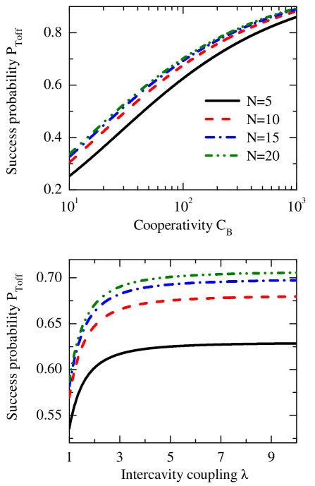
Figure 3: (Color online) Success probability, $P_{\text{Toff}}$, of our multi-qubit Toffoli-like gate as a function of (a) the cooperativity $C_{B}$ or (b) the inter-resonator-coupling strength $\lambda$, and for $N=5$ (solid black curves), $10$ (dashed red curves), $15$ (dashed-dotted blue curves), and $20$ (dashed-double dotted olive curves) three-level atoms. Here, we have assumed that $\lambda=5$ in (a) and $C_{B}=100$ in (b). In both panels, the damping rates are set as $\gamma_{g,1}=\gamma_{g,2}=\gamma$, $\gamma_{0}=\gamma_{1}=0.5\gamma$, $g_{A}=g_{B}$, $C_{B}=g_{B}^{2}/\left(\kappa\gamma\right)$, $\lambda=J/\left(\kappa\sqrt{C_{B}}\right)$, and $\alpha=\beta=1$.

In order to quantify the quality of this gate, we need to define a conditional fidelity as

$$F_{\text{Toff}}=\langle\phi|\rho_{\text{qubit}}\left(t_{\text{Toff}}\right)|\phi\rangle,$$ (35)

where $|\phi\rangle$ is assumed to be the desired state after the gate operation. Correspondingly, the gate error is characterized by $1-F_{\text{Toff}}$. Considering a generic initial state of the quartit and qutrit atoms,

$$|\Phi\rangle_{\text{ini}}=|g_{1}\rangle\left[\frac{1}{2^{N/2}}\prod_{k=1}^{N}\left(|0\rangle+|1\rangle\right)_{k}\right],$$ (36)

the success probability and the conditional fidelity is given by

$$P_{\text{Toff}} =\frac{1}{2^{N}}\sum_{n=0}^{N}C_{N}^{n}\exp\left(-\Gamma_{n}t_{\text{Toff}}\right),$$ (37)

$$F_{\text{Toff}} =\frac{1}{2^{2N}P_{\text{Toff}}}\left[\sum_{n=0}^{N}C_{N}^{n}\exp\left(-\Gamma_{n}t_{\text{Toff}}/2\right)\right]^{2},$$ (38)

respectively, with $C_{N}^{n}=N!/\left[n!\left(N-n\right)!\right]$ being the binomial coefficient. Again in the limit $\left\{G,C_{B}\right\}\gg 1$, we have $\Gamma_{n}t_{\text{T}}\ll 0$, which in turn results in

$$P_{\text{Toff}} =1-T_{p}\frac{\pi}{\sqrt{C_{B}}},$$ (39)

$$F_{\text{Toff}} =1-T_{f}\frac{\pi^{2}}{C_{B}},$$ (40)

where the scaling factors $T_{p}$ and $T_{f}$ are written as

$$T_{p}=2r+\frac{1}{r}\left[\frac{1}{2^{N}}\left(1+S_{1}\right)-1\right],$$ (41)

$$T_{f}=\frac{1}{2^{N+2}r^{2}}\left[\left(1+S_{2}\right)-\frac{1}{2^{N}}\left(1+S_{1}\right)^{2}\right],$$ (42)

respectively. Here, $r=\sqrt{\left(1/\lambda^{2}+\beta/\alpha+1\right)/2}$ with $\lambda=G/\sqrt{C_{B}}$, and $S_{x}=\sum_{n=1}^{N}C_{N}^{n}/n^{x}$ for $x=1,2$. Together with a success probability

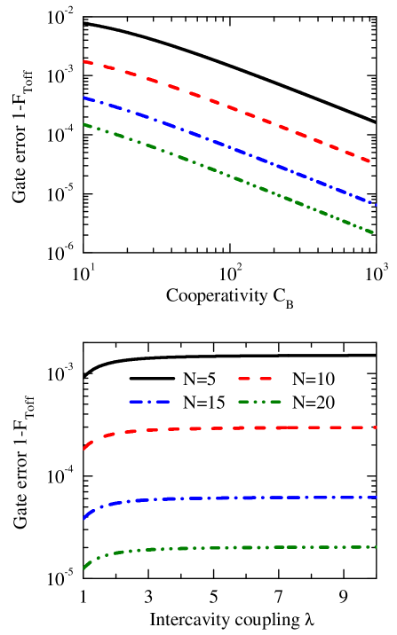
Figure 4: (Color online) Analytical results for the gate error (gate infidelity), $1-F_{\text{Toff}}$, of our multi-qubit Toffoli-like gate as a function of (a) the cooperativity $C_{B}$ or (b) the inter-resonator coupling strength $\lambda$, and for $N=5$ (solid black curves), $10$ (dashed red curves), $15$ ( dashed-dotted blue curves), and $20$ (dashed-double dotted olive curves) three-level atoms (qutrits). The other parameters are also set to be the same as in Fig. 3. There the success probability is in a one-to-one correspondence with the gate error here.

$$P_{\text{Toff}}\propto 1-1/\sqrt{C_{B}}.$$ (43)

Thus, the proposed protocol for our multi-qubit Toffoli-like gate has an error scaling as

$$1-F_{\text{Toff}}\propto 1/C_{B},$$ (44)

which is a quadratic improvement as compared to gate protocols making use of coherent unitary dynamics in cavities Sørensen and Mølmer (2003), as explained in Ref. Borregaard et al. (2015). The latter gate suffers errors from the resonator decay and atomic spontaneous emission. Instead our protocol exploits the combined effect of the unitary and dissipative processes, thus, resulting in the above improvement. In fact, the atom-resonator cooperativity $C_{B}$ could experimentally reach $>10^{4}$ in superconducting circuits Xiang et al. (2013); Niemczyk et al. (2010), thus, making the gate error very close to zero and the success probability close to unity.

The success probability is plotted as a function of either the cooperativity $C_{B}$ or the inter-resonator coupling $J$, illustrated in Fig. 3. There we have assumed that $\gamma_{g,1}=\gamma_{g,2}$, $\gamma_{0}=\gamma_{1}=0.5\gamma$, and the quartit atom is the same as the qutrit atoms, such that $\alpha=\beta=1$. Similarly, we also plot the corresponding gate error in Fig. 4. As expected, we find that increasing the cooperativity not only makes the success probability very high [see Fig. 3(a)], but it also makes the gate error very low [see Fig. 4(a)]. For example, the success probability of up to $\sim 0.9$ and the gate error of up to $\sim 2.0\times 10^{-6}$ can be achieved when $N=20$, $\lambda=5$ and $C_{B}=10^{3}$. Within the limit $\lambda\gg 1$, the $|g_{1}\rangle\leftrightarrow|e_{1}\rangle\leftrightarrow|e_{2}\rangle\leftrightarrow|g_{2}\rangle$ three-photon Raman transition off-resonantly mediated by means of the symmetric mode $a_{+}$ could be neglected, yielding $r\rightarrow\sqrt{\left(\beta/\alpha+1\right)/2}$; hence, according to Eqs. (39) and (40), the gate error is limited by an upper bound [see Fig. 4(b)], along with the corresponding success probability also upper bounded [see Fig. 3(b)].

V Heralded controlled-Z gate

Let us now consider the heralded near-deterministic realization of the two-qubit controlled-Z (CZ) gate. This gate is also known as the two-qubit controlled-sign gate, controlled-phase-flip gate, or controlled-phase gate. Specifically, the action of the CZ gate in our system can be explained as follows: Conditioned on the detection of the quartit in its ground state $|g_{1}\rangle$, the CZ gate flips the phase of the state $|11\rangle$ of an arbitrary two-qubit pure state $\mbox{$|\psi\rangle$}=c_{0}\mbox{$|00\rangle$}+c_{1}\mbox{$|01\rangle$}+c_{1}\mbox{$|01\rangle$}+c_{1}\mbox{$|11\rangle$}$ or any mixture of such states, where $c_{k}$ are the complex normalized amplitudes and the qubit states correspond to the two lowest-energy levels of the two qutrits in the resonator $B$.

It follows from Eq. (28) that, in order to completely remove the gate error, the decay rate $\Gamma_{n}$ needs to be independent of the qutrits. To this end, we retune the detunings $\delta$ and $\Delta_{e,2}$ to be

$$\frac{\delta}{\gamma} =\frac{1}{2\left(2D+G^{-1}\right)},$$ (45)

$$\frac{\Delta_{e,2}}{\gamma} =\alpha C_{B}\left(D+G^{-1}\right),$$ (46)

where $D=\sqrt{\left[1/G^{2}+\beta/\left(\alpha C_{B}\right)\right]/2}$. Thus, in the limit $\left\{G,C_{B}\right\}\gg 1$, retuning $\delta$ and $\Delta_{e,2}$ as above yields an $n$-independent decay rate

$$\Gamma_{n}=\Gamma,$$ (47)

for all $n$, while Eq. (33) is valid only for $n=0,1$. The corresponding energy shifts are given by

$$\Delta_{0}=-\frac{\Gamma D}{2},$$ (48)

and

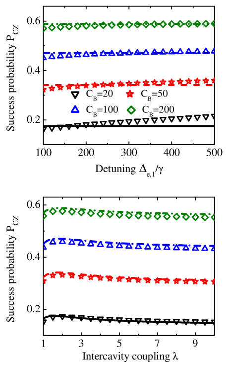
Figure 5: (Color online) Numerical simulations (marked by symbols) for the success probability, $P_{\text{CZ}}$, of the heralded CZ gate, and for the cooperativity $C_{B}=20$ (black down-triangles), $50$ (red stars), $100$ (blue up-triangles), and $200$ (olive diamonds). The success probability is displayed versus the detuning $\Delta_{e,1}$ given in terms of the overall decay rate $\gamma$ in (a), as well as versus the inter-resonator coupling strength $\lambda$ in (b). For comparison, we also plot the analytical success probability (curves), and find that the analytical results are in good agreement with the exact numerics. Here, we have assumed $\lambda=1.84$ in (a) and $\Delta_{e,1}=150\gamma$ in (b). In both panels we have set that $\gamma_{g,1}=\gamma_{g,2}=\gamma$, $\gamma_{0}=\gamma_{1}=0.5\gamma$, $\kappa=10\gamma$, $g_{A}=g_{B}$, $C_{B}=g_{B}^{2}/\left(\kappa\gamma\right)$, $\lambda=J/\left(\kappa\sqrt{C_{B}}\right)$, $\alpha=\beta=1$, $\Omega_{1}=\Delta_{e,1}/(10C_{B}^{1/4})$, and $\Omega_{2}=4\gamma C_{B}^{1/4}$.

$$\Delta_{n>0}=-\frac{\widetilde{\Omega}^{2}}{2\gamma}\frac{n\left(2D+1/G\right)}{\alpha C_{B}\left(4nD^{2}+2nD/G+1/C_{B}\right)}.$$ (49)

Subsequently, according to Eq. (28), the conditional density operator of the qutrits becomes

$$\rho_{\text{qutrit}}\left(t\right)=\sum_{n,n^{\prime}=0}^{N}e^{-i\left(\Delta_{n}-\Delta_{n^{\prime}}\right)t}\\ \mathcal{P}_{n}\left[\langle g_{1}|\rho\left(0\right)|g_{1}\rangle\right]\mathcal{P}_{n^{\prime}},$$ (50)

where the decay factor, $\exp\left(-\Gamma t\right)$, has been eliminated through a measurement conditional on the quartit atom being detected in the state $|g_{1}\rangle$. Together with single-qubit operations, we can utilize the dynamics described by the $\rho_{\text{qutrit}}\left(t\right)$ of Eq. (50) to implement a heralded CZ gate for $N=2$.

For this purpose, the duration of the driving pulse is chosen to be

$$t_{\text{CZ}}=\pi|\Delta_{2}-2\Delta_{1}+\Delta_{0}|^{-1},$$ (51)

and the unitary operation on each qubit, applied after the pulse, has the following action

$$\mathcal{U}|0\rangle=e^{i\Delta_{0}t_{\text{CZ}}/2}|0\rangle,\quad\mathcal{U}|1\rangle=e^{i\left(2\Delta_{1}-\Delta_{0}\right)t_{\text{CZ}}/2}|1\rangle,$$ (52)

so as to ensure the right phase evolution. The resulting gate is either to flip the phase of the qubit state $|11\rangle$, or to leave the otherwise qubit states unchanged. The associated success probability for any initial pure state is

$$P_{\text{CZ}}=\exp\left(-\Gamma t_{\text{CZ}}\right),$$ (53)

which can, as long as $\left\{G,C_{B}\right\}\gg 1$, be approximated as

$$P_{\text{CZ}}=1-Z_{p}\frac{\pi}{\sqrt{C_{B}}},$$ (54)

with a scaling factor

$$Z_{p}=2d+\frac{3}{2\left(2d+1/\lambda\right)}+\frac{1}{4d\left(2d+1/\lambda\right)^{2}},$$ (55)

where $d=\sqrt{\left(1/\lambda^{2}+\beta/\alpha\right)/2}$. If assuming that the desired state is $|\psi\rangle$, we can calculate the conditional fidelity for this gate via

$$F_{\text{CZ}}=\langle\psi|\left(\mathcal{U}\otimes\mathcal{U}\right)\rho_{\text{qutrit}}\left(t_{\text{CZ}}\right)\left(\mathcal{U}\otimes\mathcal{U}\right)^{{\dagger}}|\psi\rangle,$$ (56)

and then can directly find $F_{\text{CZ}}=1$. This implies that with the single-qubit operation, we achieve a more significant improvement than that shown in Eq. (44), and, thus, by decreasing $\Omega_{1}$ and increasing $\Delta_{e,1}$, an arbitrarily small gate error can even be achievable.

In order to confirm the heralded CZ gate, we now perform numerical simulations exactly using, instead of the effective master equation in Eq. (III), the full zero-temperature master equation, given by Eq. (13), for the density operator $\rho_{T}\left(t\right)$ of the total system initially in

$$|\Psi\rangle_{\text{ini}}=|\Phi\rangle_{\text{ini}}\otimes|\text{vac}\rangle,$$ (57)

with $|\text{vac}\rangle$ being the vacuum state of the coupled resonators and $|\Phi\rangle_{\text{ini}}$ is given in Eq. (36). The numerical simulations calculate the success probability $P_{\text{CZ}}$, the conditional density operator $\rho_{\text{qutrit}}\left(t_{\text{CZ}}\right)$ and fidelity $F_{\text{CZ}}$ using the expressions below:

$$P_{\text{CZ}}=\sum_{n=0,1,2}\text{Tr}\left[\left(|g_{1}\rangle\langle g_{1}|\otimes\mathcal{P}_{n}\otimes\mathcal{I}\right)\rho_{T}\left(t_{\text{CZ}}\right)\right],$$ (58)

$$\rho_{\text{qutrit}}\left(t_{CZ}\right)=\frac{1}{P_{\text{CZ}}}\text{Tr}_{\text{cav}}\left[\langle g_{1}|\rho_{T}\left(t_{\text{CZ}}\right)|g_{1}\rangle\right],$$ (59)

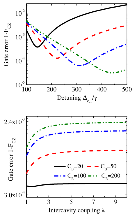
Figure 6: (Color online) Numerical simulations for the gate error, $1-F_{\text{CZ}}$, of the heralded CZ gate, and for the cooperativity $C_{B}=$20, 50, 100, and 200. Upon setting the same parameters as used in Fig. 5, the gate error is displayed versus the detuning $\Delta_{e,1}/\gamma$ in (a), as well as versus the inter-resonator coupling strength $\lambda$ in (b). There is a one-to-one correspondence between the gate error here and the numerically calculated success probability $P_{\text{CZ}}$ in Fig. 5.

$$F_{\text{CZ}}=\langle\psi|\left(\mathcal{U}\otimes\mathcal{U}\right)\rho_{\text{qutrit}}\left(t_{\text{CZ}}\right)\left(\mathcal{U}\otimes\mathcal{U}\right)^{{\dagger}}|\psi\rangle,$$ (60)

where Tr and $\text{Tr}_{\text{cav}}$ are trace operations over the total system and the resonators, respectively, and $\mathcal{I}$ is an identity operator related to the two resonators. For the simulations, we assume that $\gamma_{g,1}=\gamma_{g,2}$, $\gamma_{0}=\gamma_{1}=0.5\gamma$, and $\alpha=\beta=1$; moreover, we take $\kappa=10\gamma$, $\Omega_{1}=\Delta_{e,1}/(10C_{B}^{1/4})$, $\Omega_{2}=4\gamma C_{B}^{1/4}$, and determine the detunings $\delta$ and $\Delta_{e,2}$ according to Eqs. (45) and (46), respectively. Then, we calculate the success probability $P_{\text{CZ}}$ and the gate error $1-F_{\text{CZ}}$, as a function of either the detuning $\Delta_{e,1}$ or the inter-resonator coupling $J$, for different cooperativities Johansson et al. (2012, 2013). The numerical results (marked by symbols) are plotted in Fig. 5 for the success probability and in Fig. 6 for the gate error. The analytical success probability, which we use curves to represent, is also plotted in Fig. 5, and shows good agreement with the exact results. In Fig. 6(a) we find that as the detuning $\Delta_{e,1}$ increases, the gate error first decreases and then increases. This is because, in addition to suppressing the error from the $|e_{1}\rangle\rightarrow|g_{1}\rangle$ decay (see the Appendix), such an increase in $\Delta_{e,1}$, however, increases the driving strength $\Omega_{1}=\Delta_{e,1}/(10C_{B}^{1/4})$, and hence the non-adiabatic error. There is a trade-off between the two errors. Again within the limit $\lambda\gg 1$, the off-resonant Raman transition could be removed as before, yielding $d\rightarrow\sqrt{\beta/\left(2\alpha\right)}$. As a result, one finds that the scaling factor, given by Eq. (55), is equal to

$$Z_{p}\rightarrow 2d+\frac{3}{4d}+\frac{1}{16d^{3}}.$$ (61)

Hence, when $\lambda$ is sufficiently large, both the success probability and the gate error will be independent of $\lambda$, illustrated in Figs. 5(b) and 6(b). It should be noted that to calculate the success probability in Fig. 5(a), and the gate error in Fig. 6(a), we have chosen $\lambda=1.84$, because this value can lead to the shortest driving pulse for the two-qubit gate if $\alpha=\beta$.

Finally, we note that the energy shifts, $\Delta_{n}$, for both Toffoli-like and CZ gates involve only the ground states, because the effective master equation (III) is obtained by adiabatically eliminating the excited states. According to the effective Hamiltonian of Eq. (19), a quantum state, with $n$, of the qutrit atoms has an energy shift, $\Delta_{n}$. Consequently, a dynamical phase, $\exp(-i\Delta_{n}t)$, can be imposed by choosing the appropriate evolution times for a given quantum state. Thus, the quantum gates, including the multi-qubit Toffoli-like (see Table II) and two-qubit CZ gates (Table III), are realized by choosing appropriate evolution times.

VI conclusions

We have described a method for performing a heralded near-deterministic controlled phase gates in two distant resonators in the presence of decoherence, including the two-qubit controlled-Z (CZ) gate and its multi-qubit-controlled generalization known, which can be referred to as a Toffoli-like gate. Our proposal is a generalization of the single-resonator method introduced by Borregaard et al. Borregaard et al. (2015). The method in our paper uses an auxiliary microwave-driven four-level atom (quartit) inside one resonator to serve as both an intra-resonator photon source and a detector, and, thus, to control and also herald the gates on atomic qutrits inside the other resonator. In addition to the quantum gate fidelity scalings, which are superior to traditional cavity-assisted deterministic gates, this method demonstrates a macroscopically-distant herald for controlled quantum gates, and at the same time avoids the difficulty in individually addressing a microwave-driven atom. We note that the original method of Ref. Borregaard et al. (2015) is based on the heralding and operational atoms coupled to the same resonator mode acting as a cavity bus. Here, we are not applying this cavity bus.

The operator formalism used in our paper to calculate the effective Hamiltonian [i.e., Eq. (15)] and the effective Lindblad operators [i.e., Eq. (16)] follows the approach in Ref. Reiter and Sørensen (2012). The dynamical behavior of the system can be fairly-well approximated by the effective master equation. For example, the results obtained respectively by using the full and effective master equations in Figs. 4 and 6 in Ref. Reiter and Sørensen (2012), or in Figs. 5 and 6 in our paper, are in good agreement. The physics of this approximation can be understood by the simple qutrit atom in Fig. 2. A direct picture is that the three-level atom in state $|0\rangle$ is first excited to the state $|2\rangle$, then can go to the state $|1\rangle$ by an atomic decay, or can go back to the state $|0\rangle$ also by another atomic decay. If starting in the state $|1\rangle$, the atom has a similar behavior. Roughly speaking, there exists an indirect interaction between the states $|0\rangle$ and $|1\rangle$, as well as the direct interaction between the states $|0\rangle$, $|1\rangle$, and the state $|2\rangle$, mediated by the atomic decays. Thus, after adiabatically eliminating the state $|2\rangle$, the energy shifts of the states $|0\rangle$, $|1\rangle$, and even a direct interaction between them, would be induced by the atomic decays. Upon combining the above processes, mediated by the atom decays with the coherent drives and other interactions, the effective master equation was obtained here in analogy to that in Ref. Reiter and Sørensen (2012).

We have also proposed a circuit-QED system with superconducting qutrits and quartits implementing the proposed protocol as shown in Fig. 1. Our circuit includes two coupled transmission-line resonators, which are linearly coupled via a SQUID. These resonators can be coupled to qudits via a capacitance. For example, we assumed a phase quartit coupled to one of the resonators serving a herald, and $N$ identical flux qutrits coupled to the other resonator for performing the controlled phase gates. Typically, the length of a transmission-line resonator can be of up to the order of cm Sillanpää et al. (2007), but the size of a superconducting atoms is of $\sim\mu$m Xiang et al. (2013).

We assume realistic parameters from experiments with superconducting quantum circuits Niemczyk et al. (2010); Sillanpää et al. (2007). Specifically: $\gamma/2\pi=10$ MHZ, $\kappa/2\pi=6$ MHz, $C_{A}=C_{B}=170$ ($\alpha=\beta=1$), $\Delta_{e,1}/2\pi=420$ MHz, $\Omega_{1}/2\pi=70$ MHz, $\lambda=1.84$, $J/2\pi=144$ MHz, and $\Omega_{2}/2\pi=87$ MHz. The implementation of the CZ gate with these parameters can result in a success probability of $\sim 0.55$, a gate error of $\sim 0.006$, and a gate time of $\sim 6~{}\mu$s. These gate performance parameters are quite good for a coupled-resonator system. Indeed by increasing the capacitance of the capacitor between the TLRs, it is possible to achieve a stronger $J$ Fitzpatrick et al. (2016) and, thus, a smaller gate error and a shorter gate time. Furthermore, the decoherence time $T_{2}$ of a flux qubit can be improved to $\sim 85~{}\mu$s Yan et al. (2016), which is much larger than $6~{}\mu$s. This justifies neglecting such decoherence effect on the flux qutrits. But for a phase qubit, $T_{2}$ reaches $\sim 1~{}\mu$s, which is smaller than $6~{}\mu$s Martinis (2009). Nevertheless, the phase quartit in our protocol works only as an auxiliary atom to herald the quantum gate by measuring the $|g_{1}\rangle$ population on which the decoherence, quantified $T_{2}$, has no effect. Hence, such decoherence of both phase quartit and flux qutrits can be effectively neglected in our protocol.

Another possible implementation can be based on ultracold atoms coupled to nanoscale optical cavities. In this situation, the atoms ${}^{87}\text{Rb}$ can be used for both quartit and qutrit atoms Borregaard et al. (2015); Thompson et al. (2013); Tiecke et al. (2014). Furthermore, nanoscale optical cavities have been realized by the use of defects in a two dimensional photonic crystal, and one can place such nanocavities very close to each other to directly couple them by evanescent fields Notomi et al. (2008), or one can use a common waveguide (a quantum bus) to indirectly couple such cavities Sato et al. (2012).

Although we have chosen to discuss the specific case of two coupled resonators, this description may be extended to a coupled-cavity array Hartmann et al. (2008); Zhou et al. (2008a, b); Lu et al. (2014); Qin and Nori (2016). Hence, it would enable applications such as scalable quantum information processing and long-distance quantum communication.

VII acknowledgments

W.Q. is supported by the Basic Research Fund of the Beijing Institute of Technology under Grant No. 20141842005. X.W. is supported by the China Scholarship Council (Grant No. 201506280142). A.M. and F.N. acknowledge the support of a grant from the John Templeton Foundation. F.N. was also partially supported by the RIKEN iTHES Project, the MURI Center for Dynamic Magneto-Optics via the AFOSR award number FA9550-14-1-0040, the IMPACT program of JST, CREST grant No. JPMJCR1676, a Grant-in-Aid for Scientific Research (A), the Japan Society for the Promotion of Science (KAKENHI), JSPS-RFBR grant No. 17-52-50023.

*

Appendix A Derivation of effective master equation

In this Appendix, we will derive the effective master equation by using the method in Ref. Reiter and Sørensen (2012). We start with the total Hamiltonian $H_{T}$ in the main text. Upon introducing the symmetric and antisymmetric modes, $a_{\pm}=\left(a_{A}\pm a_{B}\right)/\sqrt{2}$, of the coupled resonators, and then switching into a rotating frame with respect to

$$H_{\text{rot}}= \sum_{k=1}^{N}\left[\left(\omega_{c}+\omega_{1}-J\right)|2\rangle_{k}\langle 2|+\sum_{z=0,1}\omega_{z}|z\rangle_{k}\langle z|\right]$$

$$+\bar{\omega}|e_{1}\rangle\langle e_{1}|+\left(\bar{\omega}+\omega_{m,2}\right)|e_{2}\rangle\langle e_{2}|$$

$$+\sum_{x=1,2}\omega_{g,x}|g_{x}\rangle\langle g_{x}|+\left(\omega_{c}-J\right)\left(a_{+}^{{\dagger}}a_{+}+a_{-}^{{\dagger}}a_{-}\right),$$ (62)

where $\bar{\omega}=\omega_{m,1}+\omega_{g,1}$, the total Hamiltonian is transformed to

$$H_{T}=H_{e}+V+V^{{\dagger}},$$ (63)

as given in the main text. With the Lindblad operators in Eq. (III), we obtain the no-jump Hamiltonian of the form

$$H_{\text{NH}}= \sum_{k=1}^{N}\left\{\bar{\delta}|2\rangle_{k}\langle 2|+\frac{g_{B}}{\sqrt{2}}\left[\left(a_{+}-a_{-}\right)|2\rangle_{k}\langle 1|+\text{H.c.}\right]\right\}$$

$$+\bar{\Delta}_{e,1}|e_{1}\rangle\langle e_{1}|+\bar{\Delta}_{e,2}|e_{2}\rangle\langle e_{2}|+\bar{J}a_{+}^{{\dagger}}a_{+}$$

$$-\frac{i\kappa}{2}a_{-}^{{\dagger}}a_{-}+\frac{g_{A}}{\sqrt{2}}\left[\left(a_{+}+a_{-}\right)|e_{2}\rangle\langle g_{2}|+\text{H.c.}\right]$$

$$+\frac{\Omega_{2}}{2}\left(|e_{2}\rangle\langle e_{1}|+\text{H.c.}\right),$$ (64)

where $\bar{\Delta}_{e,1}=\Delta_{e,1}-i\gamma_{g,1}/2$, $\bar{\Delta}_{e,2}=\Delta_{e,2}-i\gamma_{g,2}/2$, $\bar{\delta}=\delta-i\gamma/2$, and $\bar{J}=2J-i\kappa/2$. Following the formalism in Ref. Reiter and Sørensen (2012), the effective Hamiltonian and Lindblad operators are given, respectively, by

$$H_{\text{eff}}=\frac{1}{2}V^{{\dagger}}\left[H_{\text{NH}}^{-1}+\left(H_{\text{NH}}^{-1}\right)^{{\dagger}}\right]V,$$ (65)

$$L_{\text{eff}}^{j}=L_{j}H_{\text{NH}}^{-1}V.$$ (66)

To proceed, we work within the single-excitation subspace and, after a straightforward calculation, obtain

$$\Delta_{n}=-\frac{\Omega_{1}}{2\sqrt{\gamma_{g,1}}}\text{Re}\left(r_{g_{1},n}\right),$$ (67)

$$r_{+,n}=\frac{\Omega_{1}\widetilde{\Omega}_{m}\sqrt{C_{A}}}{4\widetilde{J}\mathcal{X}_{n}\sqrt{2\gamma}}\left(i\widetilde{\delta}+2nC_{B}\right),$$ (68)

$$r_{-,n}=-\frac{\Omega_{1}\widetilde{\Omega}_{m}\sqrt{C_{A}}}{2\mathcal{X}_{n}\sqrt{2\gamma}}\left(\widetilde{\delta}-nC_{B}/\widetilde{J}\right),$$ (69)

$$r_{g_{1},n}= \frac{\Omega_{1}\sqrt{\gamma_{g,1}}}{2\gamma\mathcal{X}_{n}}\bigg{[}i\widetilde{\delta}\widetilde{\Delta}_{e,2}+\left(C_{A}\widetilde{\delta}+nC_{B}\widetilde{\Delta}_{e,2}\right)$$

$$\times\left(1-i/2\widetilde{J}\right)-2nC_{A}C_{B}/\widetilde{J}\bigg{]},$$ (70)

$$r_{g_{2},n}=-\frac{\Omega_{1}\widetilde{\Omega}_{m}\sqrt{\gamma_{g,2}}}{4\gamma\mathcal{X}_{n}}\left\{i\widetilde{\delta}+nC_{B}\left[1-i/(2\widetilde{J})\right]\right\},$$ (71)

$$r_{k,n}=-\frac{\Omega_{1}\widetilde{\Omega}_{m}\sqrt{\gamma_{k}C_{A}C_{B}}}{4\gamma\mathcal{X}_{n}}\left[1+i/(2\widetilde{J})\right],$$ (72)

where $C_{A}=g_{A}^{2}/\left(\kappa\gamma\right)$, $\widetilde{\Delta}_{e,1}=\Delta_{e,1}/\gamma-i\gamma_{g,1}/\left(2\gamma\right)$, $\widetilde{J}=2J/\kappa-i/2$, $\widetilde{\Omega}_{2}=\Omega_{2}/\gamma$, $Z=\widetilde{\Delta}_{e,1}\widetilde{\Delta}_{e,2}-\left(\widetilde{\Omega}_{m}/2\right)^{2}$, $\mathcal{X}_{n}=iZ\widetilde{\delta}+\left(C_{A}\widetilde{\delta}\widetilde{\Delta}_{e,2}+nC_{B}Z\right)\left[1-i/(2\widetilde{J})\right]-2nC_{A}C_{B}\widetilde{\Delta}_{e,1}/\widetilde{J}$, and $k=0,1$. In the limit $\Omega_{2}\ll\Delta_{e,1}$, we can make a Taylor expansion around $\Omega_{2}/\Delta_{e,1}=0$, yielding

$$\Delta_{n}=-\frac{\Omega_{1}^{2}}{4\Delta_{e,1}}-\frac{\widetilde{\Omega}^{2}}{4\gamma}\text{Re}\left\{\frac{1}{\mathcal{Y}_{n}}\left\{i\widetilde{\delta}+nC_{B}\left[1-\frac{i}{2\widetilde{J}}\right]\right\}\right\},$$ (73)

$$r_{+,n}=\frac{\widetilde{\Omega}\sqrt{C_{A}}}{2\widetilde{J}\mathcal{Y}_{n}\sqrt{2\gamma}}\left(i\widetilde{\delta}+2nC_{B}\right),$$ (74)

$$r_{-,n}=-\frac{\widetilde{\Omega}\sqrt{C_{A}}}{\mathcal{Y}_{n}\sqrt{2\gamma}}\left(i\widetilde{\delta}-nC_{B}/\widetilde{J}\right),$$ (75)

$$r_{g_{1},n}=\frac{\Omega_{1}\sqrt{\gamma_{g,1}}}{2\Delta_{e,1}}+\frac{\widetilde{\Omega}\sqrt{\widetilde{\gamma}_{g,1}}}{2\gamma\mathcal{Y}_{n}}\left\{i\widetilde{\delta}+nC_{B}\left[1-\frac{i}{2\widetilde{J}}\right]\right\},$$ (76)

$$r_{g_{2},n}=-\frac{\widetilde{\Omega}\sqrt{\gamma_{g,2}}}{2\gamma\mathcal{Y}_{n}}\left\{i\widetilde{\delta}+nC_{B}\left[1-i/(2\widetilde{J})\right]\right\},$$ (77)

$$r_{k,n}=-\frac{\widetilde{\Omega}\sqrt{\gamma_{k}C_{A}C_{B}}}{2\gamma\mathcal{Y}_{n}}\left[1+i/(2\widetilde{J})\right],$$ (78)

where $\widetilde{\Omega}=\Omega_{1}\Omega_{2}/\left(2\Delta_{e,1}\right)$, $\widetilde{\gamma}_{g,1}=\gamma_{g,1}\Omega^{2}_{2}/\left(4\Delta_{e,1}^{2}\right)$, and $\mathcal{Y}_{n}=i\widetilde{\delta}\widetilde{\Delta}_{e,2}+\left(C_{A}\widetilde{\delta}+nC_{B}\widetilde{\Delta}_{e,2}\right)\left[1-i/(2\widetilde{J})\right]-2nC_{A}C_{B}/\widetilde{J}$. In Eq. (73), the term, $-\Omega_{1}^{2}/\left(4\Delta_{e,1}\right)$, of $\Delta_{n}$ can be removed because it has no effect on the phase gates. Meanwhile, in Eq. (76), we find that the $|e_{1}\rangle\rightarrow|g_{1}\rangle$ decay is suppressed by increasing $\Delta_{e,1}$, such that the second term of $r_{g_{1},n}$ can be removed as long as $\widetilde{\gamma}_{g,1}\ll 1$. Thus, Eqs. (73)–(78), under the assumption that $\kappa\ll J$, reduce to Eqs. (20) and (III) in the main text.

References

- Nielsen and Chuang (2010) M. A. Nielsen and I. L. Chuang, Quantum Computation and Quantum Information (Cambridge University Press, 2010).
- Buluta et al. (2011) I. Buluta, S. Ashhab, and F. Nori, “Natural and artificial atoms for quantum computation,” Rep. Prog. Phys. 74, 104401 (2011).
- Xiang et al. (2013) Z. L. Xiang, S. Ashhab, J. Q. You, and F. Nori, “Hybrid quantum circuits: Superconducting circuits interacting with other quantum systems,” Rev. Mod. Phys. 85, 623 (2013).
- (4) D. A. Lidar and K. B. Whaley, “Decoherence-Free Subspaces and Subsystems”, in Irreversible Quantum Dynamics, F. Benatti and R. Floreanini (Eds.), pp. 83-120 (Springer Lecture Notes in Physics vol. 622, Berlin, 2003).
- Devitt et al. (2013) S. J. Devitt, W. J. Munro, and K. Nemoto, “Quantum error correction for beginners,” Rep. Prog. Phys. 76, 076001 (2013).
- Bose et al. (1999) S. Bose, P. L. Knight, M. B. Plenio, and V. Vedral, “Proposal for teleportation of an atomic state via cavity decay,” Phys. Rev. Lett. 83, 5158–5161 (1999).
- Chimczak et al. (2005) G. Chimczak, R. Tanaś, and A. Miranowicz, “Teleportation with insurance of an entangled atomic state via cavity decay,” Phys. Rev. A 71, 032316 (2005).
- Kraus et al. (2008) B. Kraus, H. P. Büchler, S. Diehl, A. Kantian, A. Micheli, and P. Zoller, “Preparation of entangled states by quantum Markov processes,” Phys. Rev. A 78, 042307 (2008).
- Verstraete et al. (2009) F. Verstraete, M. M. Wolf, and J. I. Cirac, “Quantum computation and quantum-state engineering driven by dissipation,” Nat. Phys. 5, 633–636 (2009).
- Krauter et al. (2011) H. Krauter, C. A. Muschik, K. Jensen, W. Wasilewski, J. M. Petersen, J. I. Cirac, and E. S. Polzik, “Entanglement generated by dissipation and steady state entanglement of two macroscopic objects,” Phys. Rev. Lett. 107, 080503 (2011).
- Kastoryano et al. (2011) M. J. Kastoryano, F. Reiter, and A. S. Sørensen, “Dissipative preparation of entanglement in optical cavities,” Phys. Rev. Lett. 106, 090502 (2011).
- Reiter and Sørensen (2012) F. Reiter and A. S. Sørensen, “Effective operator formalism for open quantum systems,” Phys. Rev. A 85, 032111 (2012).
- Shen et al. (2011) L.-T. Shen, X.-Y. Chen, Z.-B. Yang, H.-Z. Wu, and S.-B. Zheng, “Steady-state entanglement for distant atoms by dissipation in coupled cavities,” Phys. Rev. A 84, 064302 (2011).
- Reiter et al. (2012) F. Reiter, M. J. Kastoryano, and A. S. Sørensen, “Driving two atoms in an optical cavity into an entangled steady state using engineered decay,” New J. Phys. 14, 053022 (2012).
- Lin et al. (2013) Y. Lin, J. P. Gaebler, F. Reiter, T. R. Tan, R. Bowler, A. S. Sørensen, D. Leibfried, and D. J. Wineland, “Dissipative production of a maximally entangled steady state of two quantum bits,” Nature (London) 504, 415–418 (2013).
- Sweke et al. (2013) R. Sweke, I. Sinayskiy, and F. Petruccione, “Dissipative preparation of large W states in optical cavities,” Phys. Rev. A 87, 042323 (2013).
- Reiter et al. (2013) F. Reiter, L. Tornberg, G. Johansson, and A. S. Sørensen, “Steady-state entanglement of two superconducting qubits engineered by dissipation,” Phys. Rev. A 88, 032317 (2013).
- Su et al. (2014) S.-L. Su, X.-Q. Shao, H.-F. Wang, and S. Zhang, “Scheme for entanglement generation in an atom-cavity system via dissipation,” Phys. Rev. A 90, 054302 (2014).
- Davis et al. (2016) E. Davis, G. Bentsen, and M. Schleier-Smith, “Approaching the Heisenberg limit without single-particle detection,” Phys. Rev. Lett. 116, 053601 (2016).
- Schönleber et al. (2015) D. W. Schönleber, A. Eisfeld, M. Genkin, S. Whitlock, and S. Wüster, “Quantum simulation of energy transport with embedded Rydberg aggregates,” Phys. Rev. Lett. 114, 123005 (2015).
- Schempp et al. (2015) H. Schempp, G. Günter, S. Wüster, M. Weidemüller, and S. Whitlock, “Correlated exciton transport in Rydberg-dressed-atom spin chains,” Phys. Rev. Lett. 115, 093002 (2015).
- Dooley et al. (2016) S. Dooley, E. Yukawa, Y. Matsuzaki, G. C. Knee, W. J. Munro, and K. Nemoto, “A hybrid-systems approach to spin squeezing using a highly dissipative ancillary system,” New J. Phys. 18, 053011 (2016).
- Ramos et al. (2016) T. Ramos, B. Vermersch, P. Hauke, H. Pichler, and P. Zoller, “Non-Markovian dynamics in chiral quantum networks with spins and photons,” Phys. Rev. A 93, 062104 (2016).
- Borregaard et al. (2015) J. Borregaard, P. Kómár, E. M. Kessler, A. S. Sørensen, and M. D. Lukin, “Heralded quantum gates with integrated error detection in optical cavities,” Phys. Rev. Lett. 114, 110502 (2015).
- You and Nori (2005) J. Q. You and F. Nori, “Superconducting circuits and quantum information,” Phys. Today 58, 42 (2005).
- Clarke and Wilhelm (2008) J. Clarke and F. K. Wilhelm, “Superconducting quantum bits,” Nature (London) 453, 1031 (2008).
- DiCarlo et al. (2010) L. DiCarlo, M. D. Reed, L. Sun, B. R. Johnson, J. M. Chow, J. M. Gambetta, L. Frunzio, S. M. Girvin, M. H. Devoret, and R. J. Schoelkopf, “Preparation and measurement of three-qubit entanglement in a superconducting circuit,” Nature (London) 467, 574 (2010).
- Lucero et al. (2012) E. Lucero, R. Barends, Y. Chen, J. Kelly, M. Mariantoni, A. Megrant, P. O Malley, D. Sank, A. Vainsencher, J. Wenner, Y. Yin, A. N. Cleland, and J. M. Martinis, “Computing prime factors with a Josephson phase qubit quantum processor,” Nat. Phys. 8, 719 (2012).
- Georgescu et al. (2014) I. M. Georgescu, S. Ashhab, and F. Nori, “Quantum simulation,” Rev. Mod. Phys. 86, 153 (2014).
- You and Nori (2003) J. Q. You and F. Nori, “Quantum information processing with superconducting qubits in a microwave field,” Phys. Rev. B 68, 064509 (2003).
- Blais et al. (2004) A. Blais, R.-S. Huang, A. Wallraff, S. M. Girvin, and R. J. Schoelkopf, “Cavity quantum electrodynamics for superconducting electrical circuits: An architecture for quantum computation,” Phys. Rev. A 69, 062320 (2004).
- You and Nori (2011) J. Q. You and F. Nori, “Atomic physics and quantum optics using superconducting circuits,” Nature (London) 474, 589 (2011).
- Liu et al. (2005) Y. X. Liu, J. Q. You, L. F. Wei, C. P. Sun, and F. Nori, “Optical selection rules and phase-dependent adiabatic state control in a superconducting quantum circuit,” Phys. Rev. Let. 95, 087001 (2005).
- Deppe et al. (2008) F. Deppe, M. Mariantoni, E. P. Menzel, A. Marx, S. Saito, K. Kakuyanagi, H. Tanaka, T. Meno, K. Semba, H. Takayanagi, E. Solano, and R. Gross, “Two-photon probe of the Jaynes-Cummings model and controlled symmetry breaking in circuit QED,” Nat. Phys. 4, 686 (2008).
- Yoshihara et al. (2017) F. Yoshihara, T. Fuse, S. Ashhab, K. Kakuyanagi, S. Saito, and K. Semba, “Superconducting qubit coscillator circuit beyond the ultrastrong-coupling regime,” Nat. Phys. 13, 44–47 (2017).
- Sørensen and Mølmer (2003) A. S. Sørensen and K. Mølmer, “Measurement induced entanglement and quantum computation with atoms in optical cavities,” Phys. Rev. Lett. 91, 097905 (2003).
- Martinis et al. (2002) J. M. Martinis, S. Nam, J. Aumentado, and C. Urbina, “Rabi oscillations in a large Josephson-junction qubit,” Phys. Rev. Lett. 89, 117901 (2002).
- Neeley et al. (2009) M. Neeley, M. Ansmann, R. C. Bialczak, M. Hofheinz, E. Lucero, A. D. O’Connell, D. Sank, H. Wang, J. Wenner, A. N. Cleland, M. R. Geller, and J. M. Martinis, “Emulation of a quantum spin with a superconducting phase qudit,” Science 325, 722–725 (2009).
- Fitzpatrick et al. (2016) M. Fitzpatrick, N. M. Sundaresan, A. C. Y. Li, J. Koch, and A. A Houck, “Observation of a dissipative phase transition in a one-dimensional circuit qed lattice,” arXiv:1607.06895 (2016).
- Nori (2009) F. Nori, “Quantum football,” Science 325, 689–690 (2009).
- Martinis (2009) J. M. Martinis, “Superconducting phase qubits,” Quantum Inf. Process. 8, 81–103 (2009).
- Liu (2014) Y. X. Liu, “Selection rules in superconducting artificial atoms,” AAPPS Bull. 24, 5–8 (2014).
- Yu et al. (2004) Y. Yu, D. Nakada, J. C. Lee, B. Singh, D. S. Crankshaw, T. P. Orlando, K. K. Berggren, and W. D. Oliver, “Energy relaxation time between macroscopic quantum levels in a superconducting persistent-current qubit,” Phys. Rev. Lett. 92, 117904 (2004).
- Imamoǧlu et al. (1999) A. Imamoǧlu, D. D. Awschalom, G. Burkard, D. P. DiVincenzo, D. Loss, M. Sherwin, and A. Small, “Quantum information processing using quantum dot spins and cavity QED,” Phys. Rev. Lett. 83, 4204–4207 (1999).
- Miranowicz et al. (2002) A. Miranowicz, S. K. Özdemir, Y. X. Liu, M. Koashi, N. Imoto, and Y. Hirayama, “Generation of maximum spin entanglement induced by a cavity field in quantum-dot systems,” Phys. Rev. A 65, 062321 (2002).
- Carmichael (1993) H. Carmichael, An Open Systems Approach to Quantum Optics (Springer-Verlag, 1993).
- Scully and Zubairy (1997) M. O. Scully and M. S. Zubairy, Quantum Optics (Cambridge University Press, 1997).
- Breuer and Petruccione (2007) H. P. Breuer and F. Petruccione, The Theory of Open Quantum Systems (Oxford University Press, 2007).
- Clerk et al. (2010) A. A. Clerk, M. H. Devoret, S. M. Girvin, F. Marquardt, and R. J. Schoelkopf, “Introduction to quantum noise, measurement, and amplification,” Rev. Mod. Phys. 82, 1155–1208 (2010).
- (50) X. Gu, A. F. Kockum, A. Miranowicz, Y. X. Liu, and F. Nori, “Microwave photonics on superconducting quantum circuits,” in preparation .
- Wallraff et al. (2005) A. Wallraff, D. I. Schuster, A. Blais, L. Frunzio, J. Majer, M. H. Devoret, S. M. Girvin, and R. J. Schoelkopf, “Approaching unit visibility for control of a superconducting qubit with dispersive readout,” Phys. Rev. Lett. 95, 060501 (2005).
- Mallet et al. (2009) F. Mallet, F. R. Ong, A. Palacios-Laloy, F. Nguyen, P. Bertet, D. Vion, and D. Esteve, “Single-shot qubit readout in circuit quantum electrodynamics,” Nat. Phys. 5, 791–795 (2009).
- Chen et al. (2012) Y. Chen, D. Sank, P. O’Malley, T. White, R. Barends, B. Chiaro, J. Kelly, E. Lucero, M. Mariantoni, A. Megrant, C. Neill, A. Vainsencher, J. Wenner, Y. Yin, A. N. Cleland, and J. M. Martinis, “Multiplexed dispersive readout of superconducting phase qubits,” Appl. Phys. Lett. 101, 182601 (2012).
- Niemczyk et al. (2010) T. Niemczyk, F. Deppe, H. Huebl, E. P. Menzel, F. Hocke, M. J. Schwarz, J. J. Garcia-Ripoll, D. Zueco, T. Hümmer, E. Solano, A. Marx, and R. Gross, “Circuit quantum electrodynamics in the ultrastrong-coupling regime,” Nat. Phys. 6, 772–776 (2010).
- Johansson et al. (2012) J. R. Johansson, P. D. Nation, and F. Nori, “Qutip: An open-source Python framework for the dynamics of open quantum systems,” Comput. Phys. Commun. 183, 1760–1772 (2012).
- Johansson et al. (2013) J. R. Johansson, P. D. Nation, and F. Nori, “Qutip 2: A Python framework for the dynamics of open quantum systems,” Comput. Phys. Commun. 184, 1234–1240 (2013).
- Sillanpää et al. (2007) M. A. Sillanpää, J. I. Park, and R. W. Simmonds, “Coherent quantum state storage and transfer between two phase qubits via a resonant cavity,” Nature (London) 449, 438–442 (2007).
- Yan et al. (2016) F. Yan, S. Gustavsson, A. Kamal, J. Birenbaum, A. P. Sears, D. Hover, T. J. Gudmundsen, D. Rosenberg, G. Samach, S. Weber, J. L. Yoder, T. P. Orlando, J. Clarke, A. J. Kerman, and W. D. Oliver, “The flux qubit revisited to enhance coherence and reproducibility,” Nat. Commun. 7, 12964 (2016).
- Thompson et al. (2013) J. D. Thompson, T. G. Tiecke, N. P. de Leon, J. Feist, A. V. Akimov, M. Gullans, A. S. Zibrov, V. Vuletić, and M. D. Lukin, “Coupling a single trapped atom to a nanoscale optical cavity,” Science 340, 1202–1205 (2013).
- Tiecke et al. (2014) T. G. Tiecke, J. D. Thompson, N. P. de Leon, L. R. Liu, V. Vuletić, and M. D. Lukin, “Nanophotonic quantum phase switch with a single atom,” Nature (London) 508, 241–244 (2014).
- Notomi et al. (2008) M. Notomi, E. Kuramochi, and T. Tanabe, “Large-scale arrays of ultrahigh-Q coupled nanocavities,” Nat. Photon. 2, 741–747 (2008).
- Sato et al. (2012) Y. Sato, Y. Tanaka, J. Upham, Y. Takahashi, T. Asano, and S. Noda, “Strong coupling between distant photonic nanocavities and its dynamic control,” Nat. Photon. 6, 56–61 (2012).
- Hartmann et al. (2008) M. J. Hartmann, F. G. S. L. Brandão, and M. B. Plenio, “Quantum many-body phenomena in coupled cavity arrays,” Laser Photon. Rev. 2, 527–556 (2008).
- Zhou et al. (2008a) L. Zhou, Z. R. Gong, Y.-X. Liu, C. P. Sun, and F. Nori, “Controllable scattering of a single photon inside a one-dimensional resonator waveguide,” Phys. Rev. Lett. 101, 100501 (2008a).
- Zhou et al. (2008b) L. Zhou, H. Dong, Y.-X. Liu, C. P. Sun, and F. Nori, “Quantum supercavity with atomic mirrors,” Phys. Rev. A 78, 063827 (2008b).
- Lu et al. (2014) J. Lu, L. Zhou, L.-M. Kuang, and F. Nori, “Single-photon router: Coherent control of multichannel scattering for single photons with quantum interferences,” Phys. Rev. A 89, 013805 (2014).
- Qin and Nori (2016) W. Qin and F. Nori, “Controllable single-photon transport between remote coupled-cavity arrays,” Phys. Rev. A 93, 032337 (2016).