Molecular simulation of the surface tension of real fluids

Abstract

Molecular models of real fluids are validated by comparing the vapor-liquid surface tension from molecular dynamics (MD) simulation to correlations of experimental data. The considered molecular models consist of up to 28 interaction sites, including Lennard-Jones sites, point charges, dipoles and quadrupoles. They represent 38 real fluids, such as ethylene oxide, sulfur dioxide, phosgene, benzene, ammonia, formaldehyde, methanol and water, and were adjusted to reproduce the saturated liquid density, vapor pressure and enthalpy of vaporization. The models were not adjusted to interfacial properties, however, so that the present MD simulations are a test of model predictions. It is found that all of the considered models overestimate the surface tension. In most cases, however, the relative deviation between the simulation results and correlations to experimental data is smaller than 20 %. This observation corroborates the outcome of our previous studies on the surface tension of 2CLJQ and 2CLJD fluids where an overestimation of the order of 10 to 20 % was found.

I Introduction

Interfacial properties are important for many applications in process engineering, including processes like absorption, wetting, nucleation, cavitation or foaming. Experimental data on the surface tension are available for pure fluids, but the temperature range is usually limited to ambient conditions DIPPR ; DDB . Hence, it is desirable to have models which allow predicting interfacial properties of pure fluids and mixtures over a wide temperature and pressure range. Molecular modelling and simulation can be used for this purpose if the underlying force fields are accurate GMT16 .

In previous work of our group DMVH12 ; MVH12b ; MVH12 ; EVH08a ; EVH08b ; HHHV11 ; EHVH07 ; EVH08c ; SCVLH07 ; SSVH07 ; SVH08 ; HMHHV12 ; VSH01 and recent work by Vrabec and co-workers MGSV13 ; EWSV12 ; EJKMMV14 ; KNWRV12 ; TDRWKSV16 ; TRKDWSV16 a large number of molecular models for real fluids were developed. The molecular model parameters were adjusted to describe the saturated liquid density, vapor pressure and enthalpy of vaporization, which they do well. These models were also used to predict transport properties and they showed very good agreement for the shear viscosity, self diffusion coefficients and thermal conductivity of pure fluids GVH12a ; MVH12 ; EWSV12 ; TDRWKSV16 ; TRKDWSV16 and mixtures GVH12a ; PGHV13 ; GVH11 ; GVH12 ; GJMV16 . Some of the fluids discussed in the present work have recently been used to develop fundamental equation of state based on molecular simulation as well as experimental data, e.g. ethylene oxide TRKKSV15 , phosgene RV15 , hexamethyldisiloxane TDRWKSV16 and octamethylcyclotetrasiloxane TRKDWSV16 . The surface tension was not part of the parameterization and is thus strictly predictive.

In previous work systematic evaluations of the surface tension of the two center Lennard-Jones plus point quadrupole (2CLJQ) and the two center Lennard-Jones plus point dipole (2CLJD) molecular model class were conducted WHH15a ; WHH16 . These models, on average, overestimate surface tension by about 20 % and 12 %, respectively WHH16 ; WSKKHH15 . Other molecular models which have been adjusted to bulk properties, but not to interfacial properties, exhibit similar deviations NWLM11 ; EMRV13 ; ALGAJM11 ; HTM15 ; FLPMM11 ; EV15 ; SSDS09 ; ZLCMSA13 ; CMHHCS12 .

In the present work, existing molecular models are used straightforwardly. No parameters are changed. By molecular dynamics (MD) simulation, predictions of interfacial properties from bulk properties are obtained. Used in this way, molecular modeling can be compared to other approaches for predicting the surface tension from bulk data, such as phenomenological parachor correlations Sugden24 ; HV86 ; GDDR89 ; ZS97 , corresponding-states or critical-scaling expressions ZS97 ; SR95 , which are also phenomenological correlations, and other molecular methods, e.g. square gradient theory GMPBM16 and density functional theory Gross09 ; TG10 on the basis of molecular equations of state GS01 ; GV06 ; VG08 ; ALAGMJ13 .

In the present work, bulk and interfacial properties of real fluids are determined simultaneously from heterogeneous MD simulations. The simulation results are compared with correlations to experimental data, where available.

II Molecular simulation

The molecular models discussed in the present work are taken from previous work of our group DMVH12 ; MVH12b ; MVH12 ; EVH08a ; EVH08b ; HHHV11 ; EHVH07 ; EVH08c ; SCVLH07 ; SSVH07 ; SVH08 ; HMHHV12 ; VSH01 and recent work by Vrabec and co-workers MGSV13 ; EWSV12 ; EJKMMV14 ; KNWRV12 ; TDRWKSV16 ; TRKDWSV16 . The molecular models are internally rigid and consist of several Lennard-Jones sites and superimposed electrostatics. The total potential energy is given by

$$U= \sum_{i=1}^{N-1}\sum_{j=i+1}^{N}\Bigg{\{}\sum_{a=1}^{n_{i}^{\rm LJ}}\sum_{b=1}^{n_{j}^{\rm LJ}}4\epsilon_{ijab}\left[\left(\frac{\sigma_{ijab}}{r_{ijab}}\right)^{12}-\left(\frac{\sigma_{ijab}}{r_{ijab}}\right)^{6}\right]+\sum_{c=1}^{n_{i}^{e}}\sum_{d=1}^{n_{j}^{e}}\frac{1}{4\pi\epsilon_{0}}\Bigg{[}\frac{q_{ic}q_{jd}}{r_{ijcd}}$$

$$+\frac{\mu_{ic}\mu_{jd}}{r_{ijcd}^{3}}\cdot f_{1}(\omega_{i},\omega_{j})+\frac{\mu_{ic}Q_{jd}+\mu_{jd}Q_{ic}}{r_{ijcd}^{4}}\cdot f_{2}(\omega_{i},\omega_{j})+\frac{Q_{ic}Q_{jd}}{r_{ijcd}^{5}}\cdot f_{3}(\omega_{i},\omega_{j})\Bigg{]}\Bigg{\}},$$ (1)

where $\epsilon_{ijab}$ and $\sigma_{ijab}$ are the Lennard-Jones energy and size parameters, $r_{ijab}$ and $r_{ijcd}$ are site-site distances, $q_{ic}$, $q_{jd}$, $\mu_{ic}$, $\mu_{jd}$, $Q_{ic}$ and $Q_{jd}$ are the magnitude of the electrostatic interactions, i.e. the point charges, dipole and quadrupole moments, and $f_{k}(\omega_{i},\omega_{j})$ are dimensionless angle-dependent expressions in terms of the orientation $\omega_{i}$,$\omega_{j}$ of the point multipoles GG84 .

Thermodynamic properties in heterogeneous systems are very sensitive to a truncation of the intermolecular potential ZLCMSA13 ; GMT14 ; WHVH15 ; GMT15 ; WHH15 ; GMSBRF04 . For dispersive interactions, like the Lennard-Jones potential, various long range correction (LRC) approaches exist which are known to be accurate for planar fluid interfaces MWF97 ; MENT03 ; Janecek06 ; VIG07 ; IHMI12 ; TSBI14 ; WRVHH14 . The simulations in the present work use slab-based LRC techniques based on the density profile MWF97 ; Janecek06 ; WRVHH14 . For polar interactions, LRCs based on Ewald summation are typically used for the simulation of vapor-liquid interfaces HE88 ; PPD88 ; EKMW04 ; IHMI12 ; MSG15 . However, a computationally efficient slab-based LRC based on the density profile can also be used for polar molecular models WHH15 . In terms of the thermodynamic results, the different methods deliver a similar degree of accuracy for the two-center Lennard-Jones plus point dipole fluid WHH16 ; MSG15 ; EKMW04 . Therefore, the slab-based LRC technique described in previous workWHH15 is employed here both for dipolar electrostatic interactions and for dispersion.

For the present series of MD simulations, systems were considered where the vapor and liquid phases coexist with each other in direct contact, employing periodic boundary conditions, so that there are two vapor-liquid interfaces which are oriented perpendicular to the $y$ axis. The interfacial tension was computed from the deviation between the normal and the tangential diagonal components of the overall pressure tensor WTRH83 ; IK49 , i.e. the mechanical route,

$$\gamma=\frac{1}{2}\int_{-\infty}^{\infty}\text{d}y\left(p_{\text{N}}-p_{\text{T}}\right).$$ (2)

Thereby, the normal pressure $p_{\text{N}}$ is given by the $y$ component of the diagonal of the pressure tensor, and the tangential pressure $p_{\text{T}}$ was determined by averaging over $x$ and $z$ components of the diagonal of the pressure tensor. The simulations were performed with the MD code ls1 mardyn ls12013 in the canonical ensemble with $N$ = 16,000 particles. Further details on the MD simulations are given in the Appendix.

III Results and Discussion

Tab. 1 gives an overview of the molecular models investigated in the present work. All studied models are rigid, i.e. internal degrees of freedom are no accounted for. The deviations $\delta\rho^{\prime}$ and $\delta p^{\rm S}$, which are reported for the models in Tab. 1, are taken from the corresponding publications and represent relative mean deviations of the simulated values from correlations to experimental data DMVH12 ; MVH12b ; MVH12 ; EVH08a ; EVH08b ; HHHV11 ; MGSV13 ; EHVH07 ; EVH08c ; SCVLH07 ; SSVH07 ; SVH08 ; HMHHV12 ; EWSV12 ; EJKMMV14 ; KNWRV12 ; TDRWKSV16 ; TRKDWSV16 ; VSH01 . The molecular simulations in previous work were performed with the Grand Equilibrium method VH02 .

Fig. 1 shows the simulation results for the vapor pressure of ammonia, methanol, sulfur dioxide and benzene from the present work which were obtained from heterogeneous simulations; cf. the Appendix (Tab. LABEL:NCLJX_tab:data) for a complete presentation of the simulated properties. The present results for the saturated densities and the vapor pressure are in very good agreement with experimental data LS06 ; PPM92 ; RC93 ; THB93 . However, for low temperatures the uncertainties in the vapor density and vapor pressure are relatively high. This is due to the fact that a low temperatures in many cases on average less than one molecule is in the vapor phase, which yields relatively high statistical uncertainties. Similar findings were obtained for the the other fluids studied in the present work. The simulation results obtained for the vapor pressure and the saturated densities for all studied fluids are reported in Tab. LABEL:NCLJX_tab:data together with the data for the surface tension.

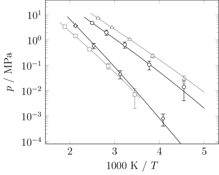
Figure 1: Vapor pressure curves of ammonia, methanol, sulfur dioxide and benzene. Solid lines represent correlations to experimental data LS06 ; PPM92 ; THB93 ; RC93 and symbols are the present simulation results: Sulfur dioxide ($\circ$), benzene ($\square$), ammonia ($\triangle$) and methanol ($\diamond$).

The relative mean deviation $\delta\gamma$ between the simulation data and the experimental data reported in Tab. 1 is calculated in the same way as the deviations for the saturated liquid density and the vapor pressure. It represents the relative mean deviation of the surface tension predicted by the molecular models from Design Institute for Physical Properties (DIPPR) correlations to experimental data

$$\left|\delta\gamma\right|=\sqrt{\frac{1}{K}\sum_{i}^{K}\left(\frac{\gamma^{\rm sim}(T_{i})-\gamma^{\rm exp}(T_{i})}{\gamma^{\rm exp}(T_{i})}\right)^{2}},$$ (3)

between the triple point temperature and 95 % of the critical temperature. By convention, the sign of $\delta\gamma$ is positive if, on average, the model overestimates the surface tension ($\delta\gamma=+\left|\delta\gamma\right|$) and negative otherwise ($\delta\gamma=-\left|\delta\gamma\right|$). Underlying experimental surface tension data are usually not available over the entire temperature range. Only for four compounds - water, methanol, ammonia, heptafluoropropane - experimental data are available over the entire temperature range. In most cases, the surface tension is measured only up to 373 K and the DIPPR correlation extrapolates these results to the critical point DIPPR ; DDB .

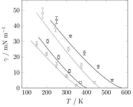
Figure 2: Surface tension as a function of the temperature. Solid lines represent DIPPR correlations to experimental data DIPPR and symbols are the present simulation results: Thiophene ($\triangledown$), ethylene oxide ($\circ$), dimethyl ether ($\square$) and heptafluoropropane ($\triangle$).

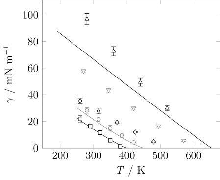
Figure 3: Surface tension as a function of the temperature. Solid lines represent DIPPR correlations to experimental data DIPPR and symbols are the present simulation results: Hydrazine ($\triangle$), methylhydrazine ($\triangledown$), 1,1-dimethylhydrazine ($\diamond$), cyanogen chloride ($\circ$) and cyanogen ($\square$). No experimental data are available for methylhydrazine and 1,1-dimethylhydrazine.

The DIPPR correlations usually agree with available experimental data within 3 %, only for dimethyl sulfide, ortho-dichlorobenzene, heptafluoropropane, cyanogen, decafluorobutane and hexamethyldisiloxane deviations of up to 5 % are reported DIPPR . For three fluids - formaldehyde, methylhydrazine and 1,1-dimethylhydrazine - no experimental data are available. The DIPPR correlations do not match the critical temperature for ethylene glycol and formic acid. Therefore, a straight line is used to connect the DIPPR correlation and the critical point of respective fluids.

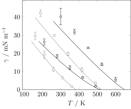
Figure 4: Surface tension as a function of the temperature. Solid lines represent DIPPR correlations to experimental data DIPPR and symbols are the present simulation results: Cyclohexanol ($\triangle$), ethyl acetate ($\square$), hexamethyldisiloxane ($\diamond$) and decafluorobutane ($\circ$).

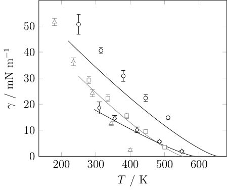
Figure 5: Surface tension as a function of the temperature. Solid lines represent DIPPR correlations to experimental data DIPPR and symbols are the present simulation results: Cyclohexanone ($\circ$), cyclohexane ($\square$), formaldehyde ($\triangle$) and octamethylcyclotetrasiloxane ($\diamond$). No experimental data are available for formaldehyde.

Figs. 2 – 9 show the surface tension for all studied fluids as a function of the temperature. The molecular simulation results are compared with DIPPR correlations to experimental data. For formaldehyde, methylhydrazine and 1,1-dimethylhydrazine no experimental data are available. The predictions of the surface tension agree reasonably well with the experimental data. Fig. 10 shows the surface tension predicted by MD simulation as a function of the experimental surface tension calculated by the DIPPR correlation DIPPR for all studied fluids. The molecular models overestimate the surface tension in all cases. The average deviation between the predictions by the molecular simulation and the experimental data is about 20 %. This is in line with results for the surface tension obtained by molecular simulation in the literature NWLM11 ; EMRV13 ; ALGAJM11 ; HTM15 ; FLPMM11 ; EV15 ; SSDS09 ; ZLCMSA13 ; CMHHCS12 ; WHH16 ; WSKKHH15 . Compared to other methods for predicting the surface tension of low-molecular fluids, molecular modeling and simulation, using models which are adjusted to bulk data, leads to relatively high deviations.

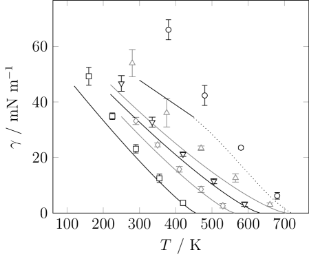
Figure 6: Surface tension as a function of the temperature. Solid lines represent DIPPR correlations to experimental data DIPPR , the dotted line connects the DIPPR correlation with the critical point of ethylene glycol, and symbols are the present simulation results: Ethylene glycol ($\circ$), ortho-dichlorobenzene ($\triangle$), chlorobenzene ($\triangledown$), benzene ($\diamond$) and phosgene ($\square$).

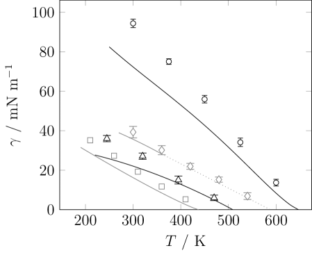
Figure 7: Surface tension as a function of the temperature. Solid lines represent DIPPR correlations to experimental data DIPPR , the dotted line connects the DIPPR correlation with the critical point of formic acid, and symbols are the present simulation results: Water ($\circ$), formic acid ($\diamond$), methanol ($\triangle$), dimethylamine ($\square$).

Several examples illustrate this: The surface tension of benzene is reproduced with a deviation of $\left|\delta\gamma\right|\approx 4\,\%$ using the corresponding-states (CS) correlation by Sastry and Rao SR95 , $\left|\delta\gamma\right|=1\,\%$ with the CS correlation by Zuo and Stenby ZS97 , and $\left|\delta\gamma\right|=8.5\,\%$ from a parachor correlation HV86 ; GDDR89 ; ZS97 ; the molecular model from Huang et al. HHHV11 has $\left|\delta\gamma\right|=11.9\,\%$. For cyclohexane, $\left|\delta\gamma\right|\approx 1\,\%$ is obtained following CS by Sastry and Rao SR95 , $\left|\delta\gamma\right|=0.7\,\%$ with CS by Zuo and Stenby ZS97 , $\left|\delta\gamma\right|=7.4\,\%$ from the parachor correlation HV86 ; GDDR89 ; ZS97 , and $\left|\delta\gamma\right|=10.8\,\%$ with the molecular model from Merker et al. MVH12b . In case of ethyl acetate, a CS correlation yields $\left|\delta\gamma\right|\approx 7\,\%$ SR95 and density functional theory with the PC-SAFT equation of state TG10 reaches $\left|\delta\gamma\right|\approx 4\,\%$, whereas the average relative deviation is $\left|\delta\gamma\right|=10.3\,\%$ for the molecular model from Eckelsbach et al. EJKMMV14 For methanol, the CS correlation by Sastry and Rao SR95 exhibits almost perfect agreement $\left|\delta\gamma\right|<1\,\%$; the molecular model by Schnabel et al. SSVH07 has $\left|\delta\gamma\right|=35.3\,\%$. Zuo and Stenby ZS97 reproduce the surface tension of isobutane with an accuracy of $\left|\delta\gamma\right|=1.6\,\%$ using their CS correlation and with $\left|\delta\gamma\right|=2.5\,\%$ using a parachor correlation HV86 ; GDDR89 ; ZS97 ; in contrast, the molecular model for isobutane from Eckl et al. EVH08b exhibits a deviation of $\left|\delta\gamma\right|=12.5\,\%$.

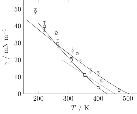
Figure 8: Surface tension as a function of the temperature. Solid lines represent DIPPR correlations to experimental data DIPPR and symbols are the present simulation results: Dimethyl sulfide ($\circ$), hydrogen cyanide ($\triangle$) and sulfur dioxide ($\square$).

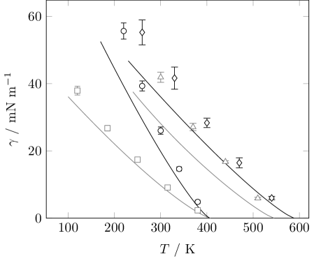
Figure 9: Surface tension as a function of the temperature. Solid lines represent DIPPR correlations to experimental data DIPPR and symbols are the present simulation results: Nitromethane ($\diamond$), acetonitrile ($\triangle$), ammonia ($\circ$) and isobutane ($\square$).

Square gradient theory with the SAFT-VR Mie equation of state, following Garrido et al. GMPBM16 , typically yields deviations of the order of 2 to 3% for the surface tension of low-molecular fluids. However, no direct comparison is possible with any of the present results.

The anisotropic united atom (AUA) force field Toxvaerd90 ; UBDBRF00 was also adjusted to bulk data only. All results for $\gamma$ from simulations with AUA models are therefore predictions of interfacial properties from bulk fluid properties. For benzene, applying the test-area method in Monte Carlo simulations with the AUA-9 sites force field, which was parameterized by Nieto Draghi and collaborators BNU07 ; NBU07 , Biscay et al. BGLM09 report a surface tension which deviates from experimental data by about $\delta\gamma\approx+4\,\%$, compared to $\delta\gamma=+11.9\,\%$ for the Huang et al. HHHV11 model. For cyclohexane BGLM09 , the AUA-9 sites model has $\delta\gamma\approx+5\,\%$, whereas for the Merker et al. MVH12b model, $\delta\gamma=+11.9\,\%$ was found in the present work. The AUA-4 model UBDBRF00 underestimates the surface tension of methanol by $\delta\gamma\approx-12\,\%$, cf. Biscay et al. BGLM11 , which compares favorably to the Schnabel et al. SSVH07 model with $\delta\gamma=+35.3\,\%$. Overall, the AUA force field is more reliable for predicting the surface tension than the models investigated in the present work BGGLM08 ; it has roughly the same accuracy as empirical parachor correlations ZS97 . However, this still makes the AUA force field less accurate than empirical CS correlations SR95 ; ZS97 and semiempirical square gradient theory GMPBM16 .

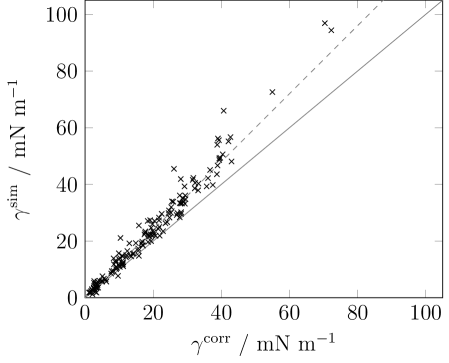
Figure 10: Predicted surface tension over the experimental surface tension based on DIPPR correlations DIPPR for the present molecular simulation results. The solid line represents perfect agreement between simulation and experiment, and the dashed line represents a deviation of 20 %.

Since molecular simulation is also computationally much more expensive than the other approaches, it cannot be recommended to predict interfacial properties from molecular models which were not previously adjusted to or, at least, validated against such data. However, a systematic overestimation of the surface tension has also been observed in density functional theory in combination with physically based equations of state TT91 ; FD93 ; W01 ; Gross09 ; LGBJ10 . To account for this overestimation, an empirical correction expression is often employed, which is formally attributed to the presence of capillary waves and decreases the surface tension. Without this correction term, which was adjusted to fit the experimental surface tension values of the n-alkane series Gross09 , density functional theory would deviate from the surface tension of real fluids in a similar way as the molecular models mentioned above. In square gradient theory, the influence parameter, which controls the magnitude of the surface excess free energy, is also adjusted to surface tension data.

Table 1: Molecular models discussed in the present work. The deviations $\delta\rho^{\prime}$ and $\delta p^{\rm s}$ as given in respective publications and $\delta\gamma$ is the root mean square relative deviation between predictions by the present MD simulations and DIPPR correlations to experimental data DIPPR . For all considered fluids, the molecular models overestimate $\gamma$ on average. # stands for the number of the corresponding sites in the model.

Name	Formula	CAS RN	# LJ	# Charges	# Dipoles	# Quadrupoles	$\delta\rho^{\prime}$	$\delta p^{\rm s}$	$\delta\gamma$	Source
Neon	Ne	7440-01-9	1	-	-	-	0.6	2.5	20.1	Vrabec et al. VSH01
Argon	Ar	7440-37-1	1	-	-	-	0.9	2.1	31.9	Vrabec et al. VSH01
Krypton	Kr	7439-90-9	1	-	-	-	0.9	2.1	27.8	Vrabec et al. VSH01
Xenon	Xe	7440-63-3	1	-	-	-	1.4	1.7	46.9	Vrabec et al. VSH01
Methane	CH4	74-82-8	1	-	-	-	1.0	2.7	19.2	Vrabec et al. VSH01
Acetonitrile	C2H3N	75-05-8	3	-	1	-	0.1	4.7	51.7	Deublein et al. DMVH12
Cyclohexane	C6H12	110-82-7	6	-	-	-	0.3	1.7	10.8	Merker et al. MVH12b
Cyclohexanone	C6H10O	108-94-1	7	-	1	-	0.9	2.7	26.0	Merker et al. MVH12b
Cyclohexanol	C6H10OH	108-93-0	7	3	-	-	0.2	3.0	28.3	Merker et al. MVH12
Ethylene oxide	C2H4O	75-21-8	3	-	1	-	0.4	1.5	16.6	Eckl et al. EVH08a
Isobutane	C4H10	75-28-5	4	-	1	1	0.6	4.2	12.5	Eckl et al. EVH08b
Formaldehyde	CH2O	50-00-0	2	-	1	-	0.9	4.3	-	Eckl et al. EVH08b
Dimethyl ether	C2H6O	115-10-6	3	-	1	-	0.4	2.6	18.9	Eckl et al. EVH08b
Sulfur dioxide	SO2	7446-09-5	3	-	1	1	0.9	4.0	3.4	Eckl et al. EVH08b
Dimethyl sulfide	C2H6S	75-18-3	3	-	1	2	0.7	4.0	18.1	Eckl et al. EVH08b
Thiophene	C4H${}_{1}0$	110-02-1	5	-	1	1	1.2	3.8	22.4	Eckl et al. EVH08b
Hydrogen cyanide	HCN	74-90-8	2	-	1	1	1.0	7.2	51.9	Eckl et al. EVH08b
Nitromethane	CH3NO2	75-52-5	4	-	1	1	0.2	18.7	31.5	Eckl et al. EVH08b
Phosgene	COCl2	75-44-5	4	-	1	1	0.5	2.1	17.2	Huang et al. HHHV11
Benzene	C6H6	71-43-2	6	-	-	6	0.4	3.4	11.9	Huang et al. HHHV11
Chlorobenzene	C6H5Cl	108-90-7	7	-	1	5	0.9	5.0	17.8	Huang et al. HHHV11
Ortho-Dichlorobenzene	C6H4Cl2	95-50-1	8	-	1	4	0.5	6.4	34.3	Huang et al. HHHV11
Cyanogen chloride	NCCl	506-77-4	3	-	1	1	0.3	2.1	15.3	Miroshnichenko et al. MGSV13
Cyanogen	C2N2	460-19-5	4	-	-	1	0.6	13.0	2.5	Miroshnichenko et al. MGSV13
Heptafluoropropane (R227ea)	C3HF7	431-89-0	10	-	1	1	1.0	1.0	7.2	Eckl et al. EHVH07
Ammonia	NH3	7664-41-7	1	4	-	-	0.7	1.6	36.7	Eckl et al. EVH08c
Formic acid	CH2O2	64-18-6	3	4	-	-	0.8	5.1	9.5	Schnabel et al. SCVLH07
Methanol	CH3OH	67-56-1	2	3	-	-	0.6	1.1	35.3	Schnabel et al. SSVH07
Dimethylamine	C2H7N	124-40-3	3	3	-	-	0.4	6.2	28.7	Schnabel et al. SVH08
Ethylene glycol	C2H6O2	107-21-1	4	6	-	-	0.8	4.8	32.6	Huang et al. HMHHV12
Water	H2O	7732-18-5	1	3	-	-	1.1	7.2	30.7	Huang et al. HMHHV12
Hydrazine	N2H4	302-01-2	2	6	-	-	0.5	7.6	29.2	Elts et al. EWSV12
Methylhydrazine	CH6N2	60-34-4	3	3	-	-	0.2	7.0	-	Elts et al. EWSV12
1,1-Dimethylhydrazine	C2H8N2	57-14-7	4	3	-	-	1.3	3.7	-	Elts et al. EWSV12
Ethyl acetate	C4H8O2	141-78-6	6	5	-	-	0.1	4.6	10.3	Eckelsbach et al. EJKMMV14
Decafluorobutane	C4F10	355-25-9	14	14	-	-	0.5	3.5	10.3	Köster et al. KNWRV12
Hexamethyldisiloxane	C6H18OSi2	107-46-0	9	3	-	-	0.5	5.0	12.9	Thol et al. TDRWKSV16
Octamethylcyclotetrasiloxane	C8H24O2Si4	556-67-2	16	8	-	-	0.5	6.0	10.5	Thol et al. TRKDWSV16

The unfavorable performance of molecular models, compared to methods which are more abstract physically and less expensive numerically, is explained by the fact that the molecular models are entirely predictive for interfacial properties. All other methods, i.e. density functional theory, square gradient theory, and phenomenological correlations, were adjusted to surface tension data at least indirectly. Moreover, methods which are based on analytical equations of state, including molecular equations of state, fail in the vicinity of the critical point, so that $\delta\gamma$ diverges at high temperatures. Renormalization group theory has to be employed in these cases to avoid unphysical behavior TG10 ; FLVTG11 ; FLVTG13 . By molecular simulation, the (Ising class) critical scaling behavior of intermolecular pair potentials is correctly captured. Therefore, any fit of force-field parameters to VLE data over a significant temperature range always indirectly adjusts the molecular model to the critical temperature SKHKH16 .

It has been shown before that a better agreement of molecular simulation results with experimental data for the surface tension can be achieved by taking into account experimental data on the surface tension in the parameterization of the molecular models. However, improvements in the quality of the representation of the surface tension have to be traded off against losses in the quality of the representation of bulk fluid properties SKRHKH14 ; WSKKHH15 ; SKHKH16 ; WSHH16 .

IV Conclusion

In the present work, the surface tension of real fluids was determined by MD simulation. The surface tension was evaluated for 38 real fluids which were parameterized to reproduce the saturated liquid density, vapor pressure and enthalpy of vaporization. The agreement between the calculated bulk values in heterogeneous simulations and the experimental data is very good. On the basis of well described phase equilibria the surface tension was predicted. The surface tension is consistently overpredicted by the molecular models. On average the deviation is about +20 %. Such overpredictions have been reported before in the literature. The reasons should be investigated in more detail in future research.

*

Table 2: Molecular simulation results for the vapor-liquid equilibrium of the pure components from the present work. The numbers in parentheses indicate the statistical uncertainties of the last decimal digits.

$T$		$p^{\text{s}}$	$\rho^{{}^{\prime}}$	$\rho^{{}^{\prime\prime}}$	$\gamma$
K		MPa	mol l-1	mol l-1	mN m-1
Acetonitrile
300		0.005(4)	18.885(1)	0.002(1)	41.9(15)
370		0.137(38)	17.013(20)	0.053(12)	27.1(6)
440		0.839(90)	14.810(21)	0.307(58)	15.7(30)
510		2.72(14)	11.84(9)	1.09(15)	5.9(3)
Cyclohexane
280		0.008(6)	9.355(3)	0.003(1)	29.2(12)
335		0.049(8)	8.750(4)	0.017(3)	22.3(13)
390		0.270(33)	8.093(3)	0.090(9)	15.5(10)
445		0.855(34)	7.325(13)	0.273(11)	9.5(7)
510		2.387(93)	6.117(26)	0.834(41)	3.5(4)
Cyclohexanone
250		0.000(0)	9.902(8)	0.000(0)	50.6(38)
315		0.002(2)	9.327(4)	0.001(1)	40.5(12)
380		0.020(6)	8.741(5)	0.006(1)	30.8(21)
445		0.148(22)	8.118(11)	0.042(5)	22.3(13)
510		0.558(37)	7.423(14)	0.146(9)	14.8(6)
Cyclohexanol
300		0.000(0)	9.700(22)	0.000(0)	40.3(62)
375		0.009(7)	9.028(4)	0.003(1)	32.0(13)
450		0.122(20)	8.277(3)	0.034(8)	22.9(4)
525		0.633(24)	7.422(13)	0.165(12)	14.0(7)
600		2.093(91)	6.325(20)	0.575(31)	5.7(11)
Ethylene oxide
180		0.000(0)	23.230(4)	0.000(0)	48.1(33)
245		0.006(4)	21.325(6)	0.004(3)	38.6(23)
310		0.331(68)	19.323(27)	0.145(30)	25.0(13)
375		1.304(57)	16.851(13)	0.495(27)	14.3(19)
440		4.77(40)	13.39(13)	2.16(34)	3.7(11)
Isobutane
120		0.000(0)	12.654(6)	0.000(0)	37.9(13)
185		0.001(1)	11.539(3)	0.001(1)	26.7(8)
250		0.067(17)	10.383(23)	0.032(7)	17.4(5)
315		0.584(10)	8.983(28)	0.263(16)	9.1(7)
380		2.32(12)	7.112(41)	1.13(12)	2.3(4)
Formaldehyde
180		0.001(1)	31.984(54)	0.001(1)	51.6(14)
235		0.030(9)	29.228(5)	0.017(5)	36.3(15)
290		0.331(54)	26.222(77)	0.155(20)	24.2(14)
345		1.66(13)	22.594(39)	0.782(66)	12.7(9)
$T$		$p^{\text{s}}$	$\rho^{{}^{\prime}}$	$\rho^{{}^{\prime\prime}}$	$\gamma$
K		MPa	mol l-1	mol l-1	mN m-1
Dimethyl ether
205		0.016(8)	17.016(5)	0.016(4)	30.0(12)
260		0.205(39)	15.415(53)	0.100(35)	19.8(13)
315		0.95(13)	13.563(13)	0.442(38)	10.9(10)
370		3.34(35)	10.94(12)	1.70(31)	3.6(6)
Sulfur dioxide
220		0.013(8)	24.771(11)	0.007(4)	39.8(29)
265		0.106(39)	22.923(25)	0.049(14)	29.6(27)
310		0.65(17)	20.932(52)	0.278(74)	20.0(14)
355		1.95(46)	18.48(12)	0.83(19)	11.1(9)
400		4.65(26)	14.87(28)	2.30(25)	3.6(10)
Dimethyl sulfide
190		0.001(1)	19.996(5)	0.000(0)	48.6(16)
260		0.036(14)	18.300(17)	0.022(14)	36.1(10)
330		0.342(26)	16.471(18)	0.134(16)	23.6(7)
400		1.70(15)	14.315(56)	0.635(65)	11.8(13)
470		5.32(33)	10.85(26)	2.60(57)	2.1(8)
Thiophene
250		0.002(1)	13.107(7)	0.001(1)	43.6(22)
320		0.035(16)	12.168(6)	0.013(4 )	33.3(7)
390		0.263(37)	11.166(7)	0.084(9)	22.4(13)
460		1.12(11)	10.001(16)	0.342(35)	13.6(10)
530		3.13(29)	8.458(65)	1.01(16)	5.0(8)
Hydrogen cyanide
280		0.038(21)	25.756(38)	0.021(11)	34.0(11)
315		0.122(12)	24.015(12)	0.063(10)	25.5(21)
340		0.343(32)	22.589(23)	0.153(23)	19.2(12)
375		0.949(50)	20.50(12)	0.431(41)	13.2(17)
410		2.03(10)	17.766(69)	1.00(12)	7.6(7)
Nitromethane
260		0.001(1)	19.569(16)	0.001(1)	55.3(37)
330		0.030(7)	18.014(6)	0.014(6)	41.6(34)
400		0.109(22)	16.259(52)	0.044(15)	28.3(14)
470		0.826(69)	14.337(25)	0.266(32)	16.5(15)
540		2.84(26)	11.70(20)	1.06(15)	6.0(9)
Phosgene
160		0.000(0)	17.047(11)	0.000(0)	49.2(32)
225		0.007(7)	15.578(10)	0.004(3)	34.8(17)
290		0.133(34)	14.047(7)	0.058(8)	23.1(21)
355		0.937(36)	12.311(20)	0.367(8)	12.5(12)
420		3.35(33)	9.873(48)	1.46(22)	3.7(7)
$T$		$p^{\text{s}}$	$\rho^{{}^{\prime}}$	$\rho^{{}^{\prime\prime}}$	$\gamma$
K		MPa	mol l-1	mol l-1	mN m-1
Benzene
290		0.007(7)	11.208(13)	0.003(3)	33.2(13)
350		0.092(23)	10.403(7)	0.033(3)	24.3(7)
410		0.423(47)	9.523(3)	0.137(16)	15.7(10)
470		1.441(67)	8.450(19)	0.468(22)	8.5(11)
530		3.337(92)	6.884(36)	1.21(13)	2.6(9)
Chlorobenzene
250		0.004(3)	10.320(8)	0.002(2)	46.7(28)
335		0.011(6)	9.466(11)	0.005(3)	33.3(19)
420		0.122(13)	8.567(23)	0.037(2)	21.9(8)
505		0.79(14)	7.520(30)	0.222(44)	11.7(9)
590		2.91(8)	5.992(20)	0.94(7)	3.2(9)
Ortho-Dichlorobenzene
375		0.003(2)	8.472(5)	0.001(1)	36.1(51)
470		0.097(17)	7.631(3)	0.026(6)	23.4(8)
565		0.701(89)	6.647(16)	0.173(28)	12.6(15)
660		2.79(14)	5.240(33)	0.807(80)	3.0(7)
Cyanogen chloride
280		0.079(21)	19.777(13)	0.036(8)	28.3(21)
315		0.312(36)	18.490(46)	0.135(9)	21.6(16)
350		0.86(17)	17.08(39)	0.361(83)	14.9(21)
385		1.86(43)	15.27(7)	0.79(23)	9.4(17)
420		3.74(36)	12.92(9)	1.86(54)	4.2(7)
Cyanogen
260		0.094(31)	18.030(33)	0.049(21)	21.9(24)
290		0.349(95)	16.866(58)	0.168(25)	16.6(12)
320		0.79(30)	15.546(99)	0.36(17)	11.5(16)
350		2.17(34)	13.820(16)	1.04(26)	5.7(6)
380		4.40(5)	11.15(28)	2.89(40)	1.2(6)
Heptafluoropropane
200		0.002(1)	10.364(13)	0.001(1)	21.9(10)
250		0.063(10)	9.381(8)	0.031(2)	14.8(19)
300		0.466(39)	8.215(3)	0.213(21)	7.7(9)
350		1.776(68)	6.531(20)	0.938(46)	1.8(6)
Ammonia
220		0.029(2)	41.985(19)	0.015(1)	55.1(19)
260		0.233(38)	38.927(14)	0.116(23)	40.1(36)
300		1.029(80)	35.470(30)	0.467(39)	26.2(13)
340		3.080(66)	31.410(26)	1.421(43)	15.2(25)
380		7.23(15)	25.572(21)	3.86(21)	4.8(1)
$T$		$p^{\text{s}}$	$\rho^{{}^{\prime}}$	$\rho^{{}^{\prime\prime}}$	$\gamma$
K		MPa	mol l-1	mol l-1	mN m-1
Formic acid
300		0.014(10)	26.192(5)	0.007(2)	39.3(29)
360		0.072(9)	24.478(9)	0.038(14)	30.2(23)
420		0.333(28)	22.607(11)	0.169(20)	22.0(15)
480		1.14(17)	20.36(17)	0.543(61)	15.3(13)
540		3.20(25)	17.45(14)	1.57(18)	6.7(15)
Methanol
245		0.001(1)	26.175(9)	0.001(1)	36.0(16)
320		0.045(17)	23.958(6)	0.020(7)	27.1(16)
395		0.58(13)	21.317(36)	0.359(49)	14.0(20)
470		3.61(14)	17.318(91)	1.61(26)	6.0(14)
Dimethylamine
210		0.003(1)	16.653(10)	0.002(1)	35.2(13)
260		0.033(11)	15.523(4)	0.016(6)	27.3(4)
310		0.257(24)	14.279(7)	0.109(10)	19.0(2)
360		1.04(10)	12.888(6)	0.407(45)	11.8(9)
410		2.65(74)	10.814(77)	1.07(50)	5.3(18)
Ethylene glycol
380		0.005(3)	16.867(29)	0.002(1)	65.6(21)
480		0.107(60)	15.527(25)	0.028(11)	42.3(36)
580		1.144(52)	13.759(14)	0.268(9)	23.6(31)
680		5.45(58)	10.906(97)	1.44(19)	6.2(12)
Water
300		0.006(5)	56.348(12)	0.002(1)	94.0(21)
375		0.069(16)	52.650(12)	0.024(8)	75.1(13)
450		0.63(10)	48.475(11)	0.31(13)	56.9(19)
525		3.31(16)	43.412(11)	0.94(6)	34.1(21)
600		10.43(20)	36.485(46)	3.28(3)	13.7(20)
Hydrazine
280		0.000(0)	32.321(8)	0.000(0)	96.7(23)
360		0.028(10)	29.955(5)	0.010(5)	72.6(13)
440		0.358(24)	27.220(18)	0.153(19)	49.4(30)
520		2.24(64)	24.063(80)	1.16(33)	29.9(20)
Methylhydrazine
270		0.009(5)	19.384(10)	0.004(3)	57.3(13)
345		0.031(13)	17.944(6)	0.012(3)	43.1(16)
420		0.420(64)	16.358(48)	0.137(40)	29.7(12)
495		1.93(21)	14.598(16)	0.573(51)	16.7(8)
570		5.21(22)	12.21(12)	1.73(13)	5.7(9)
$T$		$p^{\text{s}}$	$\rho^{{}^{\prime}}$	$\rho^{{}^{\prime\prime}}$	$\gamma$
K		MPa	mol l-1	mol l-1	mN m-1
1,1-Dimethylhydrazine
260		0.003(2)	13.783(6)	0.001(1)	35.5(21)
315		0.045(13)	12.833(4)	0.018(6)	27.6(16)
370		0.290(14)	11.806(6)	0.101(9)	19.4(9)
425		1.03(13)	10.603(3)	0.344(40)	11.9(4)
480		2.97(19)	9.026(33)	1.10(12)	4.6(4)
Ethyl acetate
190		0.000(0)	11.726(4)	0.000(0)	42.2(19)
265		0.002(1)	10.709(18)	0.001(1)	29.9(6)
340		0.063(12)	9.636(10)	0.024(3)	19.7(9)
415		0.497(39)	8.379(6)	0.170(6)	10.9(12)
490		2.078(53)	6.584(19)	0.831(37)	3.0(7)
Decafluorobutane
260		0.077(13)	6.848(12)	0.038(7)	11.8(17)
310		0.357(6)	6.021(28)	0.157(5)	6.5(6)
360		1.329(67)	4.852(77)	0.657(43)	1.7(3)
Hexamethyldisiloxane
210		0.000(0)	5.211(31)	0.000(0)	26.3(17)
280		0.002(1)	4.788(5)	0.001(0)	18.4(9)
350		0.047(15)	4.327(8)	0.017(4)	12.1(11)
420		0.299(20)	3.771(10)	0.097(10)	6.7(4)
490		1.161(26)	3.020(25)	0.421(10)	1.8(2)
Octamethylcyclotetrasiloxane
310		0.000(0)	3.135(14)	0.000(0)	18.6(33)
355		0.004(2)	2.970(12)	0.001(0)	14.6(10)
420		0.044(14)	2.709(8)	0.013(4)	10.1(11)
485		0.217(15)	2.403(12)	0.061(4)	5.7(2)
550		0.699(12)	1.985(27)	0.211(7)	1.9(3)

Molecular simulation details

The equation of motion was solved by a leapfrog integrator [95] with a time step of $\Delta t$ = 1 fs. The elongation of the simulation volume normal to the interface was 30 nm and the thickness of the liquid film in the center of the simulation volume was 15 nm to account for finite size effects [96]. The elongation in the other spatial directions was at least 10 nm. The equilibration was executed for 500,000 time steps. The production was conducted for 2,500,000 time steps to reduce statistical uncertainties. The statistical errors were estimated to be three times the standard deviation of five block averages, each over 500,000 time steps. The saturated densities and vapor pressures were calculated as an average over the respective phases excluding the area close to the interface, i.e. the area where the first derivative of the density with respect to the $y$ coordinate deviated from zero significantly.

The cutoff radius was set to 17.5 Å and a center-of-mass cutoff scheme was employed. The Lennard-Jones interactions were corrected with a slab-based long range correction based on the density profile [66]. Electrostatic long-range interactions were approximated by a resulting effective molecular dipole and corrected with a slab-based long range correction based on the density profile [58]. The quadrupolar interactions do not need a long-range correction as they decay by $r^{-10}$, cf. Prausnitz et al. [97]

References

- [1] R. L. Rowley, W. V. Wilding, J. L. Oscarson, Y. Yang, N. A. Zundel, T. E. Daubert, and R. P. Danner. DIPPR Information and Data Evaluation Manager for the Design Institute for Physical Properties. AIChE, 2013. Version 7.0.0.
- [2] DDB - Dortmund Data Bank. 7.3.0.458 (DDB), 1.18.0.122 (Artist). DDBST GmbH, Oldenburg, 2015.
- [3] A. Ghoufi, P. Malfreyt, and D. J. Tildesley. Chem. Soc. Rev., 45(5):1387–1409, 2016.
- [4] S. Deublein, P. Metzler, J. Vrabec, and H. Hasse. Mol. Sim., 39(2):109–118, 2012.
- [5] T. Merker, J. Vrabec, and H. Hasse. Fluid Phase Equilib., 315:77–83, 2012.
- [6] T. Merker, J. Vrabec, and H. Hasse. Soft Mater., 10(1-3):3–24, 2012.
- [7] B. Eckl, J. Vrabec, and H. Hasse. Fluid Phase Equilib., 274(1–2):16–26, 2008.
- [8] B. Eckl, J. Vrabec, and H. Hasse. J. Phys. Chem. B, 112(40):12710–12721, 2008.
- [9] Y.-L. Huang, M. Heilig, H. Hasse, and J. Vrabec. AIChE J., 52(4):1043–1060, 2011.
- [10] B. Eckl, Y.-L. Huang, J. Vrabec, and H. Hasse. Fluid Phase Equilib., 260:177–182, 2007.
- [11] B. Eckl, J. Vrabec, and H. Hasse. Mol. Phys., 106:1039–1046, 2008.
- [12] T. Schnabel, M. Cortada, J. Vrabec, S. Lago, and H. Hasse. Chem. Phys. Lett., 435:268–272, 2007.
- [13] T. Schnabel, A. Srivastava, J. Vrabec, and H. Hasse. J. Phys. Chem. B, 111:9871–9878, 2007.
- [14] T. Schnabel, J. Vrabec, and H. Hasse. Fluid Phase Equilib., 263:144–159, 2008.
- [15] Y.-L. Huang, T. Merker, M. Heilig, H. Hasse, and J. Vrabec. Ind. Eng. Chem. Res., 51(21):7428–7440, 2012.
- [16] J. Vrabec, J. Stoll, and H. Hasse. J. Phys. Chem. B, 105:12126–12133, 2001.
- [17] S. Miroshnichenko, T. Grützner, D. Staak, and J. Vrabec. Fluid Phase Equilib., 354:286–297, 2013.
- [18] E. Elts, T. Windmann, D. Staak, and J. Vrabec. Fluid Phase Equilib., 322–323:79–91, 2012.
- [19] S. Eckelsbach, T. Janzen, A. Köster, S. Miroshnichenko, Y. M. Muñoz Muñoz, and J. Vrabec. In W. E. Nagel, D. B. Kröner, and M. M. Resch, editors, High Performance Computing in Science and Engineering ’14, pages 645–649. Springer, Berlin/Heidelberg, 2014.
- [20] A. Köster, P. Nandi, T. Windmann, D. Ramjugernath, and J. Vrabec. Fluid Phase Equilib., 336:104–112, 2012.
- [21] M. Thol, F. H. Dubberke, G. Rutkai, T. Windmann, A. Köster, R. Span, and J. Vrabec. Fluid Phase Equilib., 416:133–151, 2016.
- [22] M. Thol, G. Rutkai, A. Köster, F. H. Dubberke, T. Windmann, R. Span, and J. Vrabec. J. Chem. Eng. Data, 61(7):2580–2595, 2016.
- [23] G. Guevara Carrión, J. Vrabec, and H. Hasse. Int. J. Thermophys., 33:449–468, 2012.
- [24] S. Pařez, G. Guevara Carrión, H. Hasse, and J. Vrabec. Phys. Chem. Chem. Phys., 15:3985–4001, 2013.
- [25] G. Guevara Carrión, J. Vrabec, and H. Hasse. J. Chem. Phys., 134:074508, 2011.
- [26] G. Guevara Carrión, J. Vrabec, and H. Hasse. Fluid Phase Equilib., 316:46–54, 2012.
- [27] G. Guevara Carrión, T. Janzen, Y. M. Muñoz Muñoz, and J. Vrabec. J. Chem. Phys., 144:124501, 2016.
- [28] M. Thol, G. Rutkai, A. Köster, M. Kortmann, R. Span, and J. Vrabec. Chem. Eng. Sci., 121:87–99, 2015.
- [29] G. Rutkai and J. Vrabec. J. Chem. Eng. Data, 60:2895–2905, 2015.
- [30] S. Werth, M. Horsch, and H. Hasse. Fluid Phase Equilib., 392:12–18, 2015.
- [31] S. Werth, M. Horsch, and H. Hasse. J. Chem. Phys., 144:054702, 2016.
- [32] S. Werth, K. Stöbener, P. Klein, K.-H. Küfer, M. Horsch, and H. Hasse. Chem. Eng. Sci., 121:110–117, 2015.
- [33] J.-C. Neyt, A. Wender, V. Lachet, and P. Malfreyt. J. Phys. Chem. B, 115(30):9421–9430, 2011.
- [34] S. Eckelsbach, S. Miroshnichenko, G. Rutkai, and J. Vrabec. In W. E. Nagel, D. B. Kröner, and M. M. Resch (eds.), High Performance Computing in Science and Engineering ’13, pp. 635–646. Springer, Heidelberg, 2013.
- [35] C. Avendaño, T. Lafitte, A. Galindo, C. S. Adjiman, G. Jackson, and E. A. Müller. J. Phys. Chem. B, 115(38):11154–11169, 2011.
- [36] C. Herdes, T. S. Totton, and E. A. Müller. Fluid Phase Equilib., 406:91–100, 2015.
- [37] N. Ferrando, V. Lachet, J. Pérez Pellitero, A. D. Mackie, and P. Malfreyt. J. Phys. Chem. B, 115(36):10654–10664, 2011.
- [38] S. Eckelsbach and J. Vrabec. Phys. Chem. Chem. Phys., 17:27195–27203, 2015.
- [39] S. K. Singh, A. Sinha, G. Deo, and J. K. Singh. J. Phys. Chem. C, 113(17):7170–7180, 2009.
- [40] R. A. Zubillaga, A. Labastida, B. Cruz, J. C. Martínez, E. Sánchez, and J. Alejandre. J. Chem. Theory Comput., 9(3):1611–1615, 2013.
- [41] C. Caleman, P. J. van Maaren, M. Hong, J. S. Hub, L. T. Costa, and D. van der Spoel. J. Chem. Theory Comput., 8(1):61–74, 2012.
- [42] S. Sugden. J. Chem. Soc., 125:1177–1189, 1924.
- [43] J. A. Hugill and A. J. van Welsenes. Fluid Phase Equilib., 29:383–390, 1986.
- [44] K. A. M. Gasem, P. B. Dulcamara Jr., K. B. Dickson, and R. L. Robinson Jr. Fluid Phase Equilib., 53:39–50, 1989.
- [45] Y.-X. Zuo and E. H. Stenby. Canad. J. Chem. Eng., 75(6):1130–1137, 1997.
- [46] S. R. S. Sastry and K. K. Rao. Chem. Eng. J., 59:181–186, 1995.
- [47] J. M. Garrido, M. M. Piñeiro, F. J. Blas, and E. A. Müller. AIChE J., 62(5):1781–1794, 2016.
- [48] J. Groß. J. Chem. Phys., 131: 204705, 2009.
- [49] X. Tang and J. Groß. J. Supercrit. Fluids, 55(2):735–742, 2010.
- [50] J. Groß and G. Sadowski. Ind. Eng. Chem. Res., 44(4):1244–1260, 2001.
- [51] J. Groß and J. Vrabec. AIChE J., 52(3): 1194–1204, 2006.
- [52] J. Vrabec and J. Groß. J. Phys. Chem. B, 112(1):51–60, 2008.
- [53] C. Avendaño, T. Lafitte, C. S. Adjiman, A. Galindo, E. A. Müller, and G. Jackson. J. Phys. Chem. B, 117(9): 2717–2733, 2013.
- [54] C. G. Gray and K. E. Gubbins. Theory of Molecular Fluids, Vol. 1: Fundamentals. Clarendon, Oxford, 1984.
- [55] F. Goujon, P. Malfreyt, and D.-J. Tildesley. J. Chem. Phys., 140:244710, 2014.
- [56] S. Werth, M. Horsch, J. Vrabec, and H. Hasse. J. Chem. Phys., 142:107101, 2015.
- [57] F. Goujon, P. Malfreyt, and D.-J. Tildesley. J. Chem. Phys., 142:107102, 2015.
- [58] S. Werth, M. Horsch, and H. Hasse. Mol. Phys., 113(23):3750–3756, 2015.
- [59] F. Goujon, P. Malfreyt, J.-M. Simon, A. Boutin, B. Rousseau, and A. H. Fuchs. J. Chem. Phys., 121(24):12559–12571, 2004.
- [60] P. J. in ’t Veld, A. E. Ismail, and G. S. Grest. J. Chem. Phys., 127:144711, 2007.
- [61] R. E. Isele-Holder, W. Mitchell, and A. E. Ismail. J. Chem. Phys., 137:174107, 2012.
- [62] G. Mathias, B. Egwolf, M. Nonella, and P. Tavan. J. Chem. Phys., 118(24):10847–10860, 2003.
- [63] D. Tameling, P. Springer, P. Bientinesi, and A. E. Ismail. J. Chem. Phys., 140:024105, 2014.
- [64] M. Mecke, J. Winkelmann, and J. Fischer. J. Chem. Phys., 107(21):9264–9270, 1997.
- [65] J. Janeček. J. Phys. Chem. B, 110(12):6264–6269, 2006.
- [66] S. Werth, G. Rutkai, J. Vrabec, M. Horsch, and H. Hasse. Mol. Phys., 112(17):2227–2234, 2014.
- [67] J. W. Perram, H. G. Peterson, and S. W. de Leeuw. Mol. Phys., 65(4):875–893, 1988.
- [68] R. W. Hockney and J. W. Eastwood. Computer Simulations Using Particles. Taylor & Francis, Bristol, PA, USA, 1988.
- [69] S. G. Moore, M. J. Stevens, and G. S. Grest. Phys. Rev. E, 91:022309, 2015.
- [70] S. Enders, H. Kahl, M. Mecke, and J. Winkelmann. J. Mol. Liq., 115(1):29–39, 2004.
- [71] J. P. R. B. Walton, D. J. Tildesley, J. S. Rowlinson, and J. R. Henderson. Mol. Phys., 48(6):1357–1368, 1983.
- [72] J. G. Kirkwood and F. P. Buff. J. Chem. Phys., 17(3):338–343, 1949.
- [73] C. Niethammer, S. Becker, M. Bernreuther, M. Buchholz, W. Eckhardt, A. Heinecke, S. Werth, H.-J. Bungartz, C. W. Glass, H. Hasse, J. Vrabec, and M. Horsch. J. Chem. Theory Comput., 10(10):4455–4464, 2014.
- [74] J. Vrabec and H. Hasse. Mol. Phys., 100(21):3375–3383, 2002.
- [75] R. Tillner-Roth, F. Harms-Watzenberg, and H. D. Baehr. DKV-Tagungsbericht, 20:167–181, 1993.
- [76] A. Polt, B. Platzer, and G. Maurer. Chem. Tech. (Leipzig), 44(6):216–224, 1992.
- [77] K. M. de Reuck and R. J. B. Craven. Methanol, International Thermodynamic Tables of the Fluid State - 12. Blackwell Scientific, London, 1993.
- [78] E. W. Lemmon and R. Span. J. Chem. Eng. Data, 51:785–850, 2006.
- [79] S. Toxvaerd. J. Chem. Phys., 93(6):4290–4295, 1990.
- [80] Ph. Ungerer, C. Beauvais, J. Delhommelle, A. Boutin, B. Rousseau, and A. H. Fuchs. J. Chem. Phys., 112(12):5499–5510, 2000.
- [81] P. Bonnaud, C. Nieto Draghi, and Ph. Ungerer. J. Phys. Chem. B, 111(14):3730–3741, 2007.
- [82] C. Nieto Draghi, P. Bonnaud, and Ph. Ungerer. J. Phys. Chem. C, 111(43):15686–15699, 2007.
- [83] F. Biscay, A. Ghoufi, V. Lachet, and P. Malfreyt. Phys. Chem. Chem. Phys., 11(29):6132–6147, 2009.
- [84] F. Biscay, A. Ghoufi, V. Lachet, and P. Malfreyt. J. Phys. Chem. C, 115(17):8670–8683, 2011.
- [85] F. Biscay, A. Ghoufi, F. Goujon, V. Lachet, and P. Malfreyt. J. Phys. Chem. B, 112(44):13885–13897, 2008.
- [86] F Llovell, A. Galindo, F. J. Blas, and G. Jackson. J. Chem. Phys., 133:024704, 2010.
- [87] P. I. Teixeira and M. M. Telo da Gama. J. Phys.: Condens. Matter, 3(1):111–125, 1991.
- [88] J. Winkelmann. J. Phys.: Condens. Matter, 13(21):4739–4768, 2001.
- [89] P. Frodl and S. Dietrich. Phys. Rev. E, 48(5):3741–3759, 1993.
- [90] E. Forte, F. Llovell, L. F. Vega, J. P. M. Trusler, and A. Galindo. J. Chem. Phys., 134:154102, 2011.
- [91] E. Forte, F. Llovell, J. P. M. Trusler, and A. Galindo. Fluid Phase Equilib., 337:274–287, 2013.
- [92] K. Stöbener, P. Klein, M. Horsch, K. Küfer, and H. Hasse. Fluid Phase Equilib., 411:33–42, 2016.
- [93] K. Stöbener, P. Klein, S. Reiser, M. Horsch, K.-H. Küfer, and H. Hasse. Fluid Phase Equilib., 373:100–108, 2014.
- [94] S. Werth, K. Stöbener, M. Horsch, and H. Hasse. Mol. Phys., 2016, accepted.
- [95] D. Fincham. Mol. Sim., 8(3–5):165–178, 1992.
- [96] S. Werth, S. V. Lishchuk, M. Horsch, and H. Hasse. Physica A, 392(10):2359–2367, 2013.
- [97] J. M. Prausnitz, R. N. Lichtenthaler, and E. G. de Azevedo. Molecular Thermodynamics of Fluid-Phase Equilibria. Pearson Education, New Jersey, 1998.
*