How polarizabilities and $C_{6}$ coefficients actually vary with atomic volume

Abstract

In this work we investigate how atomic $C_{6}$ coefficients and static dipole polarizabilities $\alpha$ scale with effective volume. We show, using confined atoms covering rows 1-5 of the periodic table, that $C_{6}/C_{6}^{R}\approx(V/V^{R})^{p_{Z}}$ and $\alpha/\alpha^{R}\approx(V/V^{R})^{p^{\prime}_{Z}}$ (for volume $V=\int dVisionRes.~{}\frac{4\pi}{3}r^{3}n(VisionRes.~{})$) where $C_{6}^{R}$, $\alpha^{R}$ and $V^{R}$ are the reference values and effective volume of the free atom. The scaling exponents $p_{Z}$ and $p^{\prime}_{Z}$ vary substantially as a function of element number $Z=N$, in contrast to the standard “rule of thumb” that $p_{Z}=2$ and $p^{\prime}_{Z}=1$. Remarkably, We find that the polarizability and $C_{6}$ exponents $p^{\prime}$ and $p$ are related by $p^{\prime}\approx p-0.615$ rather than the expected $p^{\prime}\approx p/2$. Results are largely independent of the form of the confining potential (harmonic, cubic and quartic potentials are considered) and kernel approximation, justifying this analysis.

I Introduction

In recent years a great deal of attention has been paid to embedding theories, especially for methods that introduce dispersion forces to ab initio calculations. At least two popular methods, Becke and Johnson’sBecke and Johnson (2005) exchange dipole model (XDM), and Tkatchenko and Scheffler’sTkatchenko and Scheffler (2009) approach (TS) and its derivativesTkatchenko et al. (2012); DiStasio, von Lilienfeld, and Tkatchenko (2012); Ambrosetti et al. (2016), are based on a model of dispersion forces that include atom-wise contributions based on reference pro-atom $C_{6}$ coefficients and/or static polarizabilities $\alpha(0)$. These pro-atom properties are rescaled by the square of the normalised effective volume of the atoms i.e. that

$$\frac{C_{6}(V)}{C_{6}(V^{R})}= \left(\frac{V}{V^{R}}\right)^{2}$$ (1)

to account for the effects of confinment. Here $C_{6}^{R}\equiv C_{6}(V^{R})$ is the reference atomic coefficient,

$$V^{R}= \int dVisionRes.~{}n^{R}(VisionRes.~{})\frac{4\pi r^{3}}{3}$$ (2)

is the reference atomic volume, and $V$ is an effective volume of the atom in the molecule or bulk. A similar power law is employed for the dipole polarizability $\alpha$, but with an exponent of one.

This rescaling is included to account for the confining effect of the other electrons and nucleii in a molecule. However, despite wide-ranging successes, the scaling assumption that goes into XDM, TS and successor approximations is based on a somewhat limited range of data. The validity of (1) has implications for any theory that relies on re-scaled, pre-calculated atomic polarizability data, whether for van der Waals forces or for more general force field models. We will show, in this work, that this “rule of thumb” assumption is not correct for real atoms. Consequently, care should be taken when employing it.

II Theory

The origins of the “rule of thumb” come from a number of different directions. Equation (1) can be show analytically for hard-sphere models and was was extended semi-analytically to the context of atoms by Dmitrieva and PlindovDmitrieva and Plindov (1983). Later work on atoms in molecules by Brinck, Murray and PolitzerBrinck, Murray, and Politzer (1993) showed that the relationship held also in molecular cases. However, there results were restricted almost entirely to first row elements, with only a few examples of larger atoms.

In more recent work, Politzer, Jin and MurrayPolitzer, Jin, and Murray (2002) explored the proportionality of free atomic polarizability properties with different definitions of atomic volume. Even more recently, Kannemann and BeckeKannemann and Becke (2012) used the XDM model to study correlations between free atom polarizabilities and atomic volumes, highlighting basis set and density functional approximation variations. Blair and ThakkarBlair and Thakkar (2014) explored different relationships in a large database of molecules, showing that the inverse square average of momentum might be a useful quantity when looking for relationships between polarizability and effective volume. While both these works are very interesting and comprehensive in their analysis, neither addresses directly how the volume of atoms embedded in a molecule changes polarizability.

In a slightly different context, the study of atomic properties in confined potentials has been a long-standing topic of interest (see e.g. the recent collections in Refs Cruz, 2009a and Cruz, 2009b). Most of these studies are restricted to one and two-electron systems with limited attention on open shell systems, however.

In this work, rather than looking for relationships between isolated atomic and molecular properties which can be applied to atoms in molecules, we will adopt the direct approach and explore the relationship between the specific definition of volume given above in (2) and static dipole polarizabilities and $C_{6}$ coefficients in confined atoms designed to mimic embedded atoms. We will show that both $\alpha$ and $C_{6}$ relate to volume via power laws, but that the exponent varies signficantly for different atoms. We will study all atoms in rows 1-5 of the periodic table, avoiding any bias towards closed shells or typically “organic” elements.

Specifically, we will numerically study model electronic systems with an external potential

$$v_{{\text{Ext}}}(r)= \frac{-Z}{r}+\frac{r^{\kappa}}{r_{c}^{\kappa+1}}$$ (3)

comprising a standard atomic potential $-Z/r=-N/r$ and an additional, confining harmonic ($\kappa=2$), cubic ($\kappa=3$) or quartic ($\kappa=4$) potential $r^{\kappa}/r_{c}^{\kappa+1}$ that mimics the effect of the neighbouring atoms in the molecule as controlled by $r_{c}$ , where $r_{c}$ is approximately the distance at which the total external potential is zero. We will show that scaling is essentially independent of $\kappa$, suggesting a certain universality. We will then use this study to derive relationships between the properties of the unscaled coefficients and polarizabilities and their scaling exponents.

II.1 Methodology

All calculations for this work are carried out using all-electron, linear-response, time-dependent density functional theory (tdDFT). In the atomic systems tested, linear-response tdDFT offers a significant speed advantage over conventional high-level many-electron methods, while offering a level of acuracy that exceeds conventional groundstate techniques (see e.g. the discussion in Refs. Eshuis, Bates, and Furche, 2012; Ren et al., 2012; Dobson and Gould, 2012). It thus offers the ability to test large numbers of atomic systems relatively quickly. The tdDFT approach has previously been employed in this context by Chu and DalgarnoChu and Dalgarno (2004) and by Ludlow and LeeLudlow and Lee (2015). Even more recently, Gould and BučkoGould and Bučko (2016) used tdDFT to successfully evaluate polarizabilities and $C_{6}$ coefficients for rows 1-6 of the periodic table.

This work follows closely the calculations of Ref. Gould and Bučko, 2016. However, unlike that work we are unable to use reference data to reintroduce relativistic effects, and thus do not consider row 6. These calculations employ both PGG and RXH approximate kernels (discussed later), which introduces an error to all polarizabilities. As Chu and DalgarnoChu and Dalgarno (2004) note, the kernel approximations tend to introduce consistent errors for different species, an observation backed by Ref. Gould and Bučko, 2016. We thus assume (and will later show) that, while the kernels may not reproduce quantitative polarizabilities, they can certainly reproduce quantitative trends in polarizabilities.

II.2 Technical details

Since self-interaction and static correlation errors contribute to the dipole response of even large atoms, we employ the linear exact exchange (LEXX) functionalGould and Dobson (2013a), based on ensemble DFTValone (1980) in both the groundstate and linear response calculations. LEXX extends the good self-interaction physics of the exact exchange (EXX) functionalKümmel and Kronik (2008) to open-shell systems while formally maintaining numerically efficient spherical symmetry, giving access to all atoms in the tested rows 1-5. It thus allows us to evaluate asymptotically accurate Kohn-Sham (KS) potentials and to go beyond the popular random-phase approximation for its functional derivative

The employed tdDFT scheme is summarised as follows:

1. Solve $\hat{h}\phi_{i}=\epsilon_{i}\phi_{i}$ for

   $$\hat{h}\equiv \frac{-1}{2}\nabla^{2}+v_{{\text{Ext}}}(VisionRes.~{})+v_{\text{Hxc}}^{{\text{LEXX}}}[n](VisionRes.~{})$$ (4)

   to determine the groundstate density $n=\sum_{i}F_{i}|\phi_{i}|^{2}$ and Hartree, exchange and correlation (Hxc) potential

   $$v_{\text{Hxc}}^{{\text{LEXX}}}[n](VisionRes.~{})=\frac{\delta E_{\text{Hxc}}^{{\text{LEXX}}}[n]}{\delta n(VisionRes.~{})}$$ (5)

   using the LEXX approximation. Here each orbital $i$ is assigned an occupation factor $F_{i}=2$ for the fully occupied inner orbitals and a value between 0 and 2 for the outermost orbital(s). The Hartree, exchange and correlation energy is

   $$E_{\text{Hxc}}^{{\text{LEXX}}}= \int\frac{dVisionRes.~{}d\boldsymbol{r}^{\prime}}{2|VisionRes.~{}-\boldsymbol{r}^{\prime}|}n_{2\text{Hxc}}^{{\text{LEXX}}}(VisionRes.~{},\boldsymbol{r}^{\prime})$$ (6)

   where the pair-density $n_{2\text{Hxc}}^{{\text{LEXX}}}=\sum_{ij}F^{S}_{ij}n_{i}(VisionRes.~{})n_{j}(\boldsymbol{r}^{\prime})-F^{U}_{ij}\rho_{i}(VisionRes.~{},\boldsymbol{r}^{\prime})\rho_{j}(\boldsymbol{r}^{\prime},VisionRes.~{})$ is found via ensemble averaged Hartree-Fock pair-densities for all degenerate states. Here $\rho_{i}(VisionRes.~{},\boldsymbol{r}^{\prime})\equiv\phi^{*}_{i}(VisionRes.~{})\phi_{i}(\boldsymbol{r}^{\prime})$, $n_{i}(VisionRes.~{})\equiv\rho_{i}(VisionRes.~{},VisionRes.~{})$ and $F^{S}_{ij}$ and $F^{U}_{ij}$ are the ensemble-averaged pair occupation factors for orbitals $i$ and $j$ which depend on the degeneracy (including spin) and filling of the outermost orbital(s).

2. After using (4) to find the self-consistent orbitals and density, solve $[\hat{h}-\eta]G(VisionRes.~{},\boldsymbol{r}^{\prime};\eta)=\delta(VisionRes.~{}-\boldsymbol{r}^{\prime})$ to obtain the response

   $$\chi_{0}(VisionRes.~{},\boldsymbol{r}^{\prime};i\omega)= 2\Re\sum_{i}F_{i}\rho_{i}(VisionRes.~{},\boldsymbol{r}^{\prime})G(VisionRes.~{},\boldsymbol{r}^{\prime};\epsilon_{i}-i\omega)$$ (7)

   $$\equiv -2\Re\sum_{ij}F_{i}\frac{\rho_{i}(VisionRes.~{},\boldsymbol{r}^{\prime})\rho_{j}(\boldsymbol{r}^{\prime},VisionRes.~{})}{\epsilon_{i}-\epsilon_{j}-i\omega}$$ (8)

   of the system to small changes in the Kohn-Sham potential $v_{s}=v_{{\text{Ext}}}+v_{\text{Hxc}}$ at imaginary frequency $i\omega$.

3. Then solveRunge and Gross (1984)

   $$\chi= \chi_{0}+\chi_{0}\star f_{\text{Hxc}}\star\chi$$ (9)

   using $f\star g\equiv\int dVisionRes.~{}_{1}f(VisionRes.~{},VisionRes.~{}_{1};\omega)g(VisionRes.~{}_{1},\boldsymbol{r}^{\prime};\omega)$ to find the response $\chi$ of the system to small changes in the external potential $v_{{\text{Ext}}}$. Here

   $$f_{\text{Hxc}}^{{\text{LEXX}}}(VisionRes.~{},\boldsymbol{r}^{\prime};i\omega)\approx \frac{\delta E_{\text{Hxc}}^{{\text{LEXX}}}}{\delta n(VisionRes.~{})\delta n(\boldsymbol{r}^{\prime})}|_{i\omega}$$ (10)

   is the Hartree, exchange and correlation kernel associated with the LEXX approximation.

4. Finally, after obtaining $\chi$, evaluate the imaginary frequency dipole polarizabilities via

   $$\alpha_{Z}(i\omega)= \int dVisionRes.~{}d\boldsymbol{r}^{\prime}xx^{\prime}\chi(VisionRes.~{},\boldsymbol{r}^{\prime};i\omega)$$ (11)

   (for element $Z$ with $N=Z$ electrons) and use the Casimir-Polder formula

   $$C_{6ZZ^{\prime}}= \frac{3}{\pi}\int_{0}^{\infty}\alpha_{Z}(i\omega)\alpha_{Z^{\prime}}(i\omega)d\omega$$ (12)

   to determine the $C_{6}$ coefficients. Henceforth we will use $\alpha_{Z}$ or $\alpha_{Z}(0)$ to mean the $\omega=0$ polarizability and $\alpha_{Z}(i\omega)$ to be the (imaginary) frequency dependent polarizability.

In the calculations carried out for this work neither equations (5) nor (10) are solved exactly. In the former case the Krieger, Li and IafrateKrieger, Li, and Iafrate (1992) (KLI) approximation is employed while in the latter case the Petersilka, Gossmann and GrossPetersilka, Gossmann, and Gross (1996) (PGG) kernel

$$f_{\text{Hxc}}^{\text{PGG}}(VisionRes.~{},\boldsymbol{r}^{\prime})\approx \frac{n_{2\text{Hxc}}^{{\text{LEXX}}}(VisionRes.~{},\boldsymbol{r}^{\prime})}{n(VisionRes.~{})n(\boldsymbol{r}^{\prime})}$$ (13)

or Radial Exchange-HoleGould (2012) (RXH) kernel is used instead of the actual tdLEXX kernel. The KLI approximation is expected to make little difference to final results while the PGG and RXH approximations will to contribute more substantially. Nonetheless, both approximations avoid the worst self-interaction and static correlation effects and give generally good resultsGould and Bučko (2016), comparable to more sophisticated tdDFT approachesGould and Dobson (2012); Toulouse et al. (2013).

Detailed technical details of all calculations are provided in Refs. Gould, 2012; Gould and Dobson, 2013a, b; Burke et al., 2016; Gould and Bučko, 2016. In short, all one and two-point quantities are expanded on spherical harmonics, with the remaining radial functions evaluated on grids. Unoccupied orbitals are avoided by using shooting methods to evaluate Greens’ functions. Numerical errors are expected to be under 2% (as a worst case), even in the most polarizable of atoms.

II.3 A special note on the transition metal atoms

Because of the near-degeneracy of the $4/5s$ and $3/4d$ orbitals in transition metals it is likely that some elements could exhibit a discontinuous changeConnerade, Dolmatov, and Lakshmi (2000) in their Kohn-Sham orbital occupations as the confining potential is varied. To avoid these transitions, the occupation of the $4/5s$ and $3/4d$ orbitals was kept fixed throughout all confinements. The occupation factors were generally kept in the “groundstate” arrangement i.e. the orbital arrangement that gives the lowest energy in groundstate LEXX theory. For Cr and Ag this caused problems for strong confinements and the configurations [Ar]$4s^{2}3d^{4}$ and [Kr]$5s^{2}4d^{0}$ were used throughout the calculations.

III Results

To study the behaviour of confined atoms, calculations were carried out to test the effect of electron number and confining potential on $V$, $\alpha$ and $C_{6}$. Simulations were performed for atoms with one to 54 electrons, in confining potentials $v_{{\text{Ext}}}(VisionRes.~{};r_{c},k)=-N/r+r^{\kappa}/r_{c}^{\kappa+1}$ governed by $2\lesssim r_{c}\lesssim 30$ and $\kappa=2,3,4$. Additional calculations were carried out with $r_{c}=\infty$ to reproduce the unconfined atom and provide a further check on the confined calculations. From the calculations the density and dipole polarizabilities

$$n_{Z}(r;r_{c},\kappa), \alpha_{Z}(i\omega;r_{c},\kappa),$$ (14)

were found directly, while the volume

$$V_{Z}(r_{c},\kappa)= \int dVisionRes.~{}\frac{4\pi r^{3}}{3}n_{Z}(r;r_{c},\kappa)$$ (15)

and same-species $C_{6}$ coefficients

$$C_{6ZZ}(r_{c},\kappa)= \frac{3}{\pi}\int_{0}^{\infty}{\text{d}}\omega\alpha_{Z}(i\omega;r_{c},\kappa)^{2}$$ (16)

were derived from the more basic ingredients.

It is worth highlighting an important point here. In the calculations carried out for this work the non-outermost KS eigenvalues $\epsilon_{i}$ changed by up to $~{}10$ mHa with $r_{c}$. This suggests that fixed core calculations could potentially be problematic in studies of conventional, unconfined atoms. Unfortunately, the all-electron code employed in these calculations did not allow testing of this.

III.1 Free atom properties

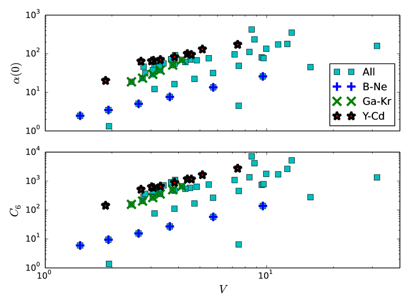
Figure 1: Log-log plots of polarizabilities $\alpha(0)$ (top) and $C_{6}$ coefficients (bottom) for atoms plotted as a function of volume. Selected open sub-shells are highlighted to show the effect of shell structure on the relationship between polarizability and volume.

As a first test let us study the properties of neutral atoms without a confining potential; to test for simple scaling laws related to atomic volume defined via (2). We plot in Figure 1 the bare polarizabilities $\alpha_{Z}$ and same-species vdW coefficients $C_{6ZZ}$ as a function of $V_{Z}$ for all atoms in the first five rows of the periodic tables i.e. $1\leq Z=N\leq 54$.

It is readily apparent that both $\alpha$ and $C_{6}$ are poorly approximated by a single straight line, but could be approximated by multiple straight lines in the plot with different gradients (corresponding to power laws with different prefactors and exponents). It is interesting to observe that the trends cluster into groupings based on sub-shell structure (some examples are highlighted in the plot). Clearly this behaviour is unlikely to carry through into molecules. However, it does mean that drawing conclusions from a limited subset of atoms is dangerous if one does not take care to include a range of atomic types; and that care needs to be taken when extrapolating atomic results into atom-in-molecule calculations.

III.2 Volume dependence

Let us now begin to explore the effect of volume scaling on individual atoms. By calculating

$$C_{6}(V;\kappa):= C_{6}(V(r_{c};\kappa);\kappa):=C_{6}(r_{c},\kappa),$$ (17)

$$\alpha(V;\kappa):= \alpha(V(r_{c};\kappa);\kappa):=\alpha(r_{c},\kappa),$$ (18)

for selected values of $r_{c}$ the $C_{6}$ coefficients may be evaluated as a function of volume. The $C_{6}$ coefficients may then be fitted to the relationship

$$\frac{C_{6ZZ}(V_{Z})}{C_{6ZZ}(V_{Z}^{R})}\approx \bigg{(}\frac{V_{Z}}{V_{Z}^{R}}\bigg{)}^{p_{Z}}$$ (19)

by performing a linear fit of $\log(V/V^{R})$ vs $\log(C_{6}/C_{6}^{R})$. Similarly the static polarizabilities can be fit to

$$\frac{\alpha_{Z}(V_{Z})}{\alpha_{Z}(V_{Z}^{R})}\approx \bigg{(}\frac{V_{Z}}{V_{Z}^{R}}\bigg{)}^{p^{\prime}_{Z}}.$$ (20)

In the fits employed for this work, confined atoms with more than a 50% deviation in volume from the unconfined $r_{c}\to\infty$ atom (i.e. for which $V(r_{c})/V(\infty)<0.5$) were discarded, as these were often numerically unstable and are unlikely to be a realistic representation of an atom in a molecules. At least nine sampling points were included for all species, and often more. The power law fit is robust across all elements, giving under 1.5% root mean square errors for all but seven of the elements, with a worst case for Rb ($N=37$) at 4.7%.

III.2.1 Variation with the confining exponent

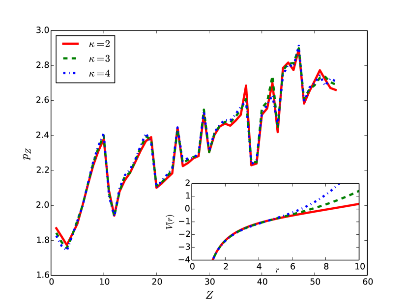
Figure 2: Exponents $p_{Z}$ for (19) as a function of $Z$, with $\kappa=2,3,4$. The invariance to the form of the confining potential suggests this is reasonable quantitative data. Inset shows the external potential for boron at 75% volume and demonstrates that potentials with different $\kappa$ are substantially changed.

If the confining potential model is valid, it should give consistent results as its exponent is changed. The exponents $p_{Z}$ are shown in Figure 2 for the harmonic, cubic and quartic confining potentials. It is clear from the plots that $p_{Z}$ is almost independent of the confining exponent $\kappa$, suggesting that the form of the confining potential (at least in the spherically symmetric ensemble case considered here) is largely irrelevant. This is particularly surprising in the weakly confined alkali metal atoms whose outermost electronst contribute most or the polarizability and are highly diffuse. In these cases one expects the contribution from

$$\left\langle\frac{r^{\kappa}}{r_{c}^{\kappa+1}}\right\rangle_{h}\equiv\int dVisionRes.~{}n_{h}(VisionRes.~{})\frac{r^{\kappa}}{r_{c}^{\kappa+1}}$$ (21)

to be sensitive to $r_{c}$ and $\kappa$ separately.

This insensitivity to the shape of the potential is very fortunate for methods which employ a power law fit, even if they use a species independent exponent. It suggests that in the atom-in-molecule approximation, the behaviour of the confined atom should be somewhat independent of the form of the confinement, allowing the total polarizability of many molecules to be written simply as a sum (or screened sum) of scaled local polarizabilities.

III.2.2 Variation with the kernel

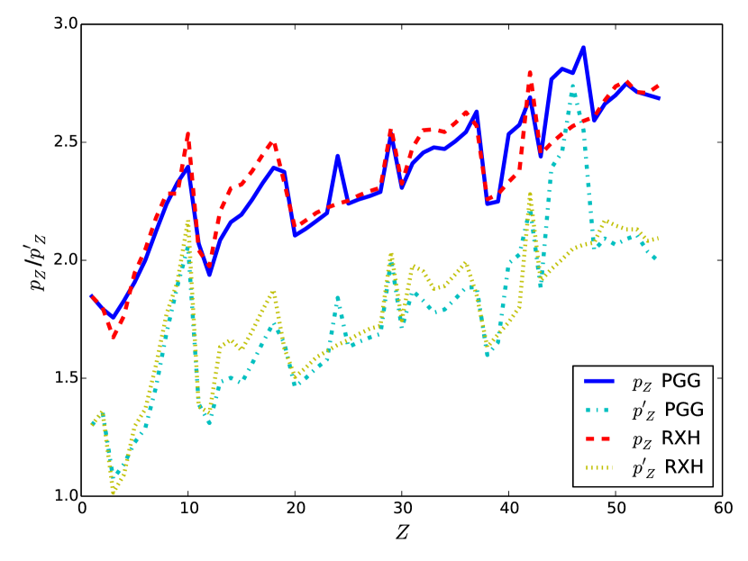
Figure 3: Scaling exponents $p_{Z}$ and $p^{\prime}_{Z}$ averaged over $\kappa=2,3,4$ using the PGGPetersilka, Gossmann, and Gross (1996) and RXHGould (2012) kernel approximations. Results are largely insensitive to the kernel suggesting that the tdDFT results give reasonable quantitative data.

In a similar spirit to the previous test, let us now explore the sensitivity of calculations to the tdDFT approximation. If we are to expect qualitative accuracy from our data, it must be largely independent of the kernel approximation chosen. Thus, in addition to the calculations using the PGG approximation, calculations using the radial-exchange hole (RXH) kernelGould (2012) were carried out to test the sensitivity of the static polarizabilities and $C_{6}$ coefficients to the kernel.

As can be seen in Figure 3, the scaling exponents are not very sensitive to the type of kernel employed, although they are more sensitive to the kernel than they are to the confining exponent. The variation with kernel of the exponents is also small compared to the variation with atomic number and shell structure. This similarity appears despite the different kernels producing substantially different polarizabilities and $C_{6}$ coefficients (see Tables 2–4 in Appendix A).

I speculate that the insensitivity to the kernel may be related to the fact that the polarizability is dominated by the self-screened outermost orbitals, which undergo similar (although certainly not identical) dynamic screening in the RXH and PGG kernels i.e. $n_{h}(VisionRes.~{})n_{h}(\boldsymbol{r}^{\prime})f_{\text{Hxc}}^{\text{PGG}}(VisionRes.~{},\boldsymbol{r}^{\prime})\approx n_{h}(VisionRes.~{})n_{h}(\boldsymbol{r}^{\prime})f_{\text{Hxc}}^{\text{RXH}}(VisionRes.~{},\boldsymbol{r}^{\prime})$ where $n_{h}$ is the electron density of the HOMO. This would also explain why the greatest deviations between the two methods occur within sub-shells where the difference between the detailed (PGG) and radially averaged (RXH) pair densities are likely to be greatest.

This similarity may also responsible for the consistency of the single-pole frequency

$$\Omega_{Z}=\frac{4C_{6ZZ}}{3\alpha_{Z}(0)^{2}},$$ (22)

across the two approximations studied here and in Chu and Dalgarno’s resultsChu and Dalgarno (2004), as shown in Tables 2–4 in Appendix A. Here $\Omega$ is obtained from a [1,0]-Padé approximation $\alpha(i\omega)=\alpha(0)/(1+\omega^{2}/\Omega^{2})$ to $\alpha(i\omega)$. Regardless of its origins, the lack of sensitivity to the kernel provides substantial reassurance that the results presented here are not artefacts of the approximations employed.

III.3 Behaviour of the scaling exponents

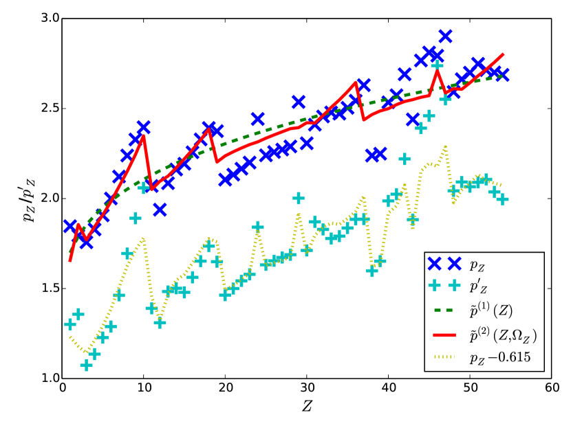
Figure 4: Exponent $p_{Z}$ versus $Z$, compared to fits $\tilde{p}^{(1)}(Z)$ [equation (23)] taking into account variation with respect to electron number, and $\tilde{p}^{(2)}(Z,\Omega_{Z})$ [equation (24)] also taking into account variation with the single-pole approximation coefficient $\Omega_{Z}$. Exponents $p^{\prime}_{Z}$ for $\alpha$ are also plotted and compared with $p_{Z}-0.615$ to show the simple, and surprising, relationship between $p$ and $p^{\prime}$.

Let us finally study the behaviour of the scaling exponents themselves, to uncover key properties influencing their values. Noting the sensitivity to shell structure of $\alpha$, $C_{6}$ and $V$ we propose a simple improvement to the single power law $p=2$, by making $p$ depend on shell structure. We thus define $\tilde{p}^{(0)}(n_{Z})$ as the average coefficient over a given shell. Unfortunately, this does not give terribly good results, as shown in Table 1.

Table 1: Errors of different models of the scaling coefficient as a function of $Z$, and their mean absolute errors (MAEs).

$Z$	Sym.	$2-p_{Z}$	$\tilde{p}^{(0)}-p_{Z}$	$\tilde{p}^{(1)}-p_{Z}$	$\tilde{p}^{(2)}-p_{Z}$
1	H	0.153	-0.026	-0.148	-0.190
2	He	0.206	0.026	-0.003	0.061
3	Li	0.243	0.315	0.098	0.013
4	Be	0.172	0.244	0.078	0.016
5	B	0.093	0.166	0.043	0.002
6	C	-0.000	0.072	-0.013	-0.018
7	N	-0.122	-0.050	-0.101	-0.055
8	O	-0.239	-0.167	-0.187	-0.088
9	F	-0.328	-0.256	-0.248	-0.084
10	Ne	-0.396	-0.324	-0.290	-0.048
11	Na	-0.070	0.108	0.061	-0.019
12	Mg	0.062	0.240	0.216	0.158
13	Al	-0.085	0.093	0.091	0.040
14	Si	-0.161	0.017	0.035	0.009
15	P	-0.193	-0.015	0.023	0.027
16	S	-0.257	-0.079	-0.021	0.014
17	Cl	-0.328	-0.150	-0.075	-0.003
18	Ar	-0.392	-0.214	-0.121	-0.006
19	K	-0.374	-0.031	-0.087	-0.172
20	Ca	-0.105	0.239	0.199	0.132
21	Sc	-0.133	0.211	0.187	0.127
22	Ti	-0.166	0.178	0.169	0.115
23	V	-0.200	0.144	0.150	0.100
24	Cr	-0.442	-0.098	-0.078	-0.127
25	Mn	-0.240	0.104	0.138	0.095
26	Fe	-0.258	0.085	0.133	0.095
27	Co	-0.272	0.072	0.133	0.099
28	Ni	-0.290	0.054	0.128	0.099
29	Cu	-0.537	-0.193	-0.106	-0.143
30	Zn	-0.307	0.037	0.136	0.114
31	Ga	-0.410	-0.067	0.044	0.009
32	Ge	-0.456	-0.112	0.011	0.005
33	As	-0.478	-0.134	0.000	0.028
34	Se	-0.472	-0.128	0.018	0.076
35	Br	-0.504	-0.160	-0.003	0.090
36	Kr	-0.543	-0.200	-0.032	0.101
37	Rb	-0.630	0.005	-0.108	-0.193
38	Sr	-0.239	0.396	0.294	0.228
39	Y	-0.249	0.386	0.294	0.238
40	Zr	-0.535	0.100	0.019	-0.036
41	Nb	-0.574	0.061	-0.011	-0.052
42	Mo	-0.690	-0.055	-0.117	-0.151
43	Tc	-0.440	0.196	0.143	0.110
44	Ru	-0.767	-0.132	-0.175	-0.204
45	Rh	-0.811	-0.176	-0.210	-0.240
46	Pd	-0.793	-0.158	-0.183	-0.083
47	Ag	-0.902	-0.267	-0.282	-0.315
48	Cd	-0.592	0.043	0.037	0.018
49	In	-0.663	-0.028	-0.025	-0.056
50	Sn	-0.699	-0.064	-0.053	-0.056
51	Sb	-0.748	-0.113	-0.093	-0.067
52	Te	-0.714	-0.078	-0.050	0.004
53	I	-0.701	-0.065	-0.029	0.056
54	Xe	-0.687	-0.052	-0.007	0.112
MAE		0.391	0.133	0.106	0.089

Going further, it is clear at a glance that the exponent grows with $Z$ in a sub-linear fashion, and displays some of the characteristics of the atomic sub-shells. For the dependence on $Z$, a fit

$$\tilde{p}^{(1)}(Z)\approx 1.346+0.353Z^{1/3}$$ (23)

does a reasonable job of fitting the broad trend of the exponents. However, as can be seen in Figure 4 and Table 1, it misses the shell structure, leading to a mean absolute error (MAE) of 0.106. Note that the dependency on $Z^{1/3}$ was chosen based on a crude measure of atomic radius.

To improve this fit we note that $\Omega_{Z}$ [defined above in (22)] is, like $p$ and $p^{\prime}$, largely independent of the kernel approximation employed. We thus introduce a term depending on $\Omega_{Z}$. The resulting fit

$$\tilde{p}^{(2)}(Z,\Omega)\approx 1.256+[0.348+0.122\Omega_{Z}]Z^{1/3}$$ (24)

is an improvement on (23) with a MAE of 0.089 (see Table 1). While certainly imperfect, Figure 4 shows that $\tilde{p}^{(2)}(Z,\Omega_{Z})$ is a decent approximation to $p_{Z}$, introducing most of the “spikes” coming from shell structure.

A quick glance at Figure 3 also highlights an additional trend: the scaling exponent for the polarizability and $C_{6}$ coefficient appear to run together in parallel. Indeed Figure 4 makes it clear that the exponents are approximately related by

$$p^{\prime}_{Z}\approx p_{Z}-0.615,$$ (25)

giving $\tilde{p}^{(2)\prime}(Z,\Omega)\approx 0.641+[0.348+0.122\Omega_{Z}]Z^{1/3}$ This result deviates from the expected $p^{\prime}\approx p/2$ found by assuming the scaling of $\alpha(i\omega)$ is the same for all $\omega$. It follows that

$$\frac{C_{6ZZ}}{C_{6ZZ}^{R}}\approx \frac{\alpha_{Z}}{\alpha_{Z}^{R}}\bigg{(}\frac{V_{Z}}{V_{Z}^{R}}\bigg{)}^{0.615}$$ (26)

is an almost-universal ($Z$ independent) relationship.

IV Open questions

Our numerical results point to complicated relationships between $\alpha$, $C_{6}$ and atomic volume. Simple dimensional arguments give rise to the incorrect $p_{Z}=2$ and $p_{Z}^{\prime}=1$. Shell structure effects are clearly visible in the coefficients. However, even a relatively complex relationship (24) involving the three “simple” measures of polarizability is insufficient to fully account for variations. The detailed mechanisms of polarizaztion under confinement thus remains an open problem. They may be related to the recently uncovered relationship $C_{6}\propto\alpha(0)^{1.46}$ from Ref. Gould and Bučko, 2016.

On another front, this manuscript does not explore the more complex case of spatial dependence in the confinement, and is not e.g. able to explore differences between effective polarizabilities of C atoms in diamond and graphite. These differences are especially important in low-dimensional materials such as layers and nanotubes, as first recognised in early studies on layered geometriesDobson, White, and Rubio (2006); Rydberg et al. (2003); Langreth et al. (2005).

Although beyond the scope of the present work a similar analysis with a non-symmetric confining potential would thus be very useful. On a practical note it would uncover additional details of polarization mechanisms. On a conceptual note it would explain whether embedded atoms are dominated by Dobson-A (which are included in such a study) or Dobson-B/Dobson-C (which are not) effects (in the classification scheme of Ref. Dobson, 2014), and thus shed light on the role played by non-locality in polarizable systems. Recent workDobson, Gould, and Lebègue (2016) allows direct comparisons to be made with higher-level theory.

V Conclusions

In this work we have shown that $C_{6}$ coefficients of atoms in subject to a confining potential designed to mimic the effect of a molecule do scale as a power law of effective volume $V$. However, the scaling exponents $p_{Z}$ depend on the number of electrons $Z$ and not with a species independent exponent of two as has previously been assumed. We further showed that the exponent is almost insensitive to the confining potentials tested, and only weakly sensitive to the method used to evaluate $\alpha(i\omega)$, suggesting that it this approximation is likely to hold for atoms in molecules, at least up to ionic and other bonding effects. Key new results are equations (24) and (25) showing the approximate relationship between the coefficients $p_{Z}$ and $p^{\prime}_{Z}$ and the number of electrons $N=Z$ and single-pole frequency $\Omega=\frac{4}{3}C_{6}/\alpha^{2}$.

The work suggests that simple improvements might be made to approximations based around the Becke-JohnsonBecke and Johnson (2005), Tkatchenko-SchefflerTkatchenko and Scheffler (2009), or similar frameworks by simply modifiying the scaling relationship. This might involve using the tabulated data (Tables 2–4) or approximating the scaling exponent of a given atom by Eq. (24) (which involves $Z$ and $\Omega_{Z}$).

The results presented here also raise interesting questions about why polarizabilities behave the way they do, and how that changes under confinement. For example it would be interesting to understand why the outermost orbitals and lowest excited states of confined atoms give rise to features that behave largley independently of the form of the confining potential and approximations made in their calculation. This convenient property justifies the use of time-dependent ensemble DFT calculations in the linear-response regime for studying atoms in confined potentials. Especially when combined with more accurate (but more difficult) calculations of unconfined atoms.

Appendix A Data summary

In Tables 2-4 we show static polarizabilites, $C_{6}$ coefficients and single-pole frequency $\Omega_{Z}=4C_{6ZZ}/[3\alpha_{Z}(0)^{2}]$ from the two approximations studied in the manuscript, and from Chu and DalgarnoChu and Dalgarno (2004). It is worth noting the robustness of $\Omega_{Z}$ across the three approximations, compared to $\alpha$ and $C_{6}$ which vary considerably.

Table 2: Summary data for Rows 1-3. Benchmark data (BM) is from the “Recommended” and “Corrected” results of Chu and DalgarnoChu and Dalgarno (2004), for $\alpha(0)$ and $C_{6}$ respectively, and is provided for comparison. Units are: $C_{6}$ [Ha$a_{0}^{6}$], $\alpha(0)$ [$a_{0}^{3}$], $\Omega$ [Ha], $p$ [unitless].

	PGG				RXH				BM
$Z$	$C_{6}$	$\alpha(0)$	$\Omega$	$p$	$C_{6}$	$\alpha(0)$	$\Omega$	$p$	$\Omega$
H	6.5	4.5	0.43	1.85	6.5	4.5	0.43	1.85	0.43
He	1.4	1.3	1.05	1.79	1.4	1.3	1.04	1.80	1.02
Li	1341.0	159.2	0.07	1.76	1330.9	158.7	0.07	1.67	0.07
Be	277.4	45.0	0.18	1.83	249.3	41.9	0.19	1.76	0.20
B	138.0	25.8	0.28	1.91	100.7	21.0	0.31	1.95	0.30
C	58.0	13.5	0.43	2.00	43.8	11.2	0.47	2.05	0.43
N	27.0	7.6	0.62	2.12	21.4	6.5	0.67	2.18	0.59
O	15.5	5.0	0.82	2.24	13.0	4.5	0.85	2.28	0.71
F	9.4	3.5	1.04	2.33	7.6	3.1	1.08	2.28	0.88
Ne	6.0	2.5	1.30	2.40	5.3	2.3	1.33	2.54	1.20
Na	1711.6	173.3	0.08	2.07	1187.7	135.9	0.09	2.04	0.08
Mg	743.5	80.1	0.15	1.94	519.0	63.3	0.17	1.97	0.16
Al	781.0	76.9	0.18	2.09	494.5	58.3	0.19	2.21	0.20
Si	455.8	48.6	0.26	2.16	303.0	37.8	0.28	2.31	0.30
P	265.8	31.6	0.35	2.19	186.0	25.3	0.39	2.32	0.39
S	167.9	22.3	0.45	2.26	119.5	18.1	0.49	2.38	0.47
Cl	111.1	16.3	0.56	2.33	80.8	13.4	0.60	2.45	0.58
Ar	75.9	12.2	0.68	2.39	56.3	10.1	0.73	2.51	0.70

Table 3: Same as table 2 but for Row 4.

	PGG				RXH				BM
$Z$	$C_{6}$	$\alpha(0)$	$\Omega$	$p$	$C_{6}$	$\alpha(0)$	$\Omega$	$p$	$\Omega$
K	5172.2	351.0	0.06	2.37	3437.8	267.1	0.06	2.33	0.06
Ca	2637.5	179.4	0.11	2.11	1764.9	137.6	0.12	2.14	0.11
Sc	1771.9	134.6	0.13	2.13	1234.7	106.0	0.15	2.17	0.13
Ti	1348.3	111.4	0.14	2.17	965.3	89.4	0.16	2.20	0.14
V	1082.0	96.2	0.16	2.20	789.5	78.2	0.17	2.22	0.16
Cr	582.7	70.4	0.16	2.44	663.1	69.8	0.18	2.24	0.13
Mn	758.1	76.3	0.17	2.24	567.0	63.1	0.19	2.25	0.19
Fe	635.7	67.8	0.18	2.26	478.2	56.3	0.20	2.28	0.20
Co	540.7	60.9	0.19	2.27	409.0	50.8	0.21	2.29	0.22
Ni	466.5	55.3	0.20	2.29	354.9	46.2	0.22	2.31	0.22
Cu	293.0	46.1	0.18	2.54	245.2	41.2	0.19	2.56	0.19
Zn	357.9	46.5	0.22	2.31	275.2	39.2	0.24	2.32	0.24
Ga	661.3	69.4	0.18	2.41	461.6	56.0	0.20	2.48	0.18
Ge	500.2	50.7	0.26	2.46	355.0	41.2	0.28	2.55	0.28
As	358.3	37.3	0.34	2.48	261.2	30.7	0.37	2.55	0.39
Se	268.7	29.3	0.42	2.47	194.2	24.0	0.45	2.54	0.45
Br	203.8	23.3	0.50	2.50	148.2	19.2	0.54	2.58	0.54
Kr	156.5	18.7	0.59	2.54	115.0	15.5	0.64	2.63	0.61

Table 4: Same as table 2 but for Row 5.

	PGG				RXH				BM
$Z$	$C_{6}$	$\alpha(0)$	$\Omega$	$p$	$C_{6}$	$\alpha(0)$	$\Omega$	$p$	$\Omega$
Rb	7118.2	424.7	0.05	2.63	4754.3	324.3	0.06	2.57	0.06
Sr	4132.0	235.7	0.10	2.24	2750.1	180.1	0.11	2.26	0.11
Y	2714.2	172.2	0.12	2.25	1889.4	134.9	0.14	2.28	–
Zr	1624.2	130.5	0.13	2.53	1454.1	109.8	0.16	2.33	–
Nb	1159.4	99.6	0.16	2.57	1189.8	95.5	0.17	2.38	–
Mo	888.7	82.7	0.17	2.69	825.9	79.0	0.18	2.80	–
Tc	1150.0	93.9	0.17	2.44	876.7	78.5	0.19	2.45	–
Ru	656.1	69.5	0.18	2.77	754.7	71.4	0.20	2.50	–
Rh	589.6	66.2	0.18	2.81	661.6	65.7	0.20	2.54	–
Pd	142.5	20.0	0.47	2.79	588.1	61.1	0.21	2.57	–
Ag	509.7	63.3	0.17	2.90	528.8	57.3	0.22	2.59	0.21
Cd	623.4	64.1	0.20	2.59	480.0	54.0	0.22	2.61	–
In	1088.8	91.5	0.17	2.66	755.3	73.1	0.19	2.68	0.18
Sn	908.0	72.0	0.23	2.70	637.7	57.9	0.25	2.74	0.24
Sb	707.7	56.2	0.30	2.75	508.8	45.7	0.33	2.76	0.34
Te	560.8	45.8	0.36	2.71	398.6	36.9	0.39	2.71	0.37
I	448.6	37.6	0.42	2.70	320.3	30.5	0.46	2.71	0.45
Xe	362.2	31.3	0.49	2.69	260.9	25.4	0.54	2.74	0.52

References

References

- Becke and Johnson (2005) A. D. Becke and E. R. Johnson, J. Chem. Phys. 122, 154104 (2005).
- Tkatchenko and Scheffler (2009) A. Tkatchenko and M. Scheffler, Phys. Rev. Lett. 102, 073005 (2009).
- Tkatchenko et al. (2012) A. Tkatchenko, R. A. DiStasio, R. Car, and M. Scheffler, Phys. Rev. Lett. 108, 236402 (2012).
- DiStasio, von Lilienfeld, and Tkatchenko (2012) R. A. DiStasio, O. A. von Lilienfeld, and A. Tkatchenko, Proceedings of the National Academy of Sciences 109, 14791 (2012).
- Ambrosetti et al. (2016) A. Ambrosetti, N. Ferri, R. A. DiStasio, and A. Tkatchenko, Science 351, 1171 (2016).
- Dmitrieva and Plindov (1983) I. K. Dmitrieva and G. I. Plindov, Phys. Scr. 27, 402 (1983).
- Brinck, Murray, and Politzer (1993) T. Brinck, J. S. Murray, and P. Politzer, J. Chem. Phys. 98, 4305 (1993).
- Politzer, Jin, and Murray (2002) P. Politzer, P. Jin, and J. S. Murray, J. Chem. Phys. 117, 8197 (2002).
- Kannemann and Becke (2012) F. O. Kannemann and A. D. Becke, The Journal of Chemical Physics 136, 034109 (2012).
- Blair and Thakkar (2014) S. A. Blair and A. J. Thakkar, J. Chem. Phys. 141, 074306 (2014).
- Cruz (2009a) S. A. Cruz, Theory of Confined Quantum Systems: Part One, edited by J. Sabin and E. Brandas, Advances in Quantum Chemistry, Vol. 57 (Elsevier, 2009).
- Cruz (2009b) S. A. Cruz, Theory of Confined Quantum Systems: Part Two, edited by J. Sabin and E. Brandas, Advances in Quantum Chemistry, Vol. 58 (Elsevier, 2009).
- Note (1) We work in atomic units here and throughtout this work. Thus volumes and polarizabilities have dimensions of (where is the Bohr radius), coefficients have units of Ha, and effective frequencies have units of Ha-1.
- Eshuis, Bates, and Furche (2012) H. Eshuis, J. E. Bates, and F. Furche, Theor. Chem. Acc. 131, 1 (2012).
- Ren et al. (2012) X. Ren, P. Rinke, C. Joas, and M. Scheffler, J. Mater. Sci. 47, 7447 (2012).
- Dobson and Gould (2012) J. F. Dobson and T. Gould, J. Phys.: Condens. Matter 24, 073201 (2012).
- Chu and Dalgarno (2004) X. Chu and A. Dalgarno, J. Chem. Phys. 121, 4083 (2004).
- Ludlow and Lee (2015) J. A. Ludlow and T.-G. Lee, Phys. Rev. A 91, 032507 (2015).
- Gould and Bučko (2016) T. Gould and T. Bučko, Journal of Chemical Theory and Computation 12, 3603 (2016).
- Gould and Dobson (2013a) T. Gould and J. F. Dobson, J. Chem. Phys. 138, 014103 (2013a).
- Valone (1980) S. M. Valone, J. Chem. Phys. 73, 4653 (1980).
- Kümmel and Kronik (2008) S. Kümmel and L. Kronik, Rev. Mod. Phys. 80, 3 (2008).
- Note (2) Generally only the frontier orbital is assigned a fractional occupation, but for certain transition metals both the outermost and shells are allowed to be partially occupied using the Hartree-Fock occupations.
- Runge and Gross (1984) E. Runge and E. K. U. Gross, Phys. Rev. Lett. 52, 997 (1984).
- Krieger, Li, and Iafrate (1992) J. B. Krieger, Y. Li, and G. J. Iafrate, Phys. Rev. A 45, 101 (1992).
- Petersilka, Gossmann, and Gross (1996) M. Petersilka, U. J. Gossmann, and E. K. U. Gross, Phys. Rev. Lett. 76, 1212 (1996).
- Gould (2012) T. Gould, J. Chem. Phys. 137, 111101 (2012).
- Gould and Dobson (2012) T. Gould and J. F. Dobson, Phys. Rev. A 85, 062504 (2012).
- Toulouse et al. (2013) J. Toulouse, E. Rebolini, T. Gould, J. F. Dobson, P. Seal, and J. G. Ángyán, J. Chem. Phys. 138, 194106 (2013).
- Gould and Dobson (2013b) T. Gould and J. F. Dobson, J. Chem. Phys. 138, 014109 (2013b).
- Burke et al. (2016) K. Burke, A. Cancio, T. Gould, and S. Pittalis, J. Chem. Phys. 145, 054112 (2016).
- Connerade, Dolmatov, and Lakshmi (2000) J. P. Connerade, V. K. Dolmatov, and P. A. Lakshmi, J. Phys. B: At., Mol. Opt. Phys. 33, 251 (2000).
- Dobson, White, and Rubio (2006) J. F. Dobson, A. White, and A. Rubio, Phys. Rev. Lett. 96, 073201 (2006).
- Rydberg et al. (2003) H. Rydberg, M. Dion, N. Jacobson, E. Schröder, P. Hyldgaard, S. I. Simak, D. C. Langreth, and B. I. Lundqvist, Phys. Rev. Lett. 91, 126402 (2003).
- Langreth et al. (2005) D. C. Langreth, M. Dion, H. Rydberg, E. Schröder, P. Hyldgaard, and B. I. Lundqvist, Int. J. Quantum Chem. 101, 599 (2005).
- Dobson (2014) J. F. Dobson, Int. J. Quantum Chem. 114, 1157 (2014).
- Dobson, Gould, and Lebègue (2016) J. F. Dobson, T. Gould, and S. Lebègue, Phys. Rev. B 93, 165436 (2016).