Cycles and Intractability in a Large Class
of Aggregation Rules

Abstract

We introduce the $(j,k)$-Kemeny rule – a generalization of Kemeny’s voting rule that aggregates $j$-chotomous weak orders into a $k$-chotomous weak order. Special cases of $(j,k)$-Kemeny include approval voting, the mean rule and Borda mean rule, as well as the Borda count and plurality voting. Why, then, is the winner problem computationally tractable for each of these other rules, but intractable for Kemeny? We show that intractability of winner determination for the $(j,k)$-Kemeny rule first appears at the $j=3$, $k=3$ level. The proof rests on a reduction of max cut to a related problem on weighted tournaments, and reveals that computational complexity arises from the cyclic part in the fundamental decomposition of a weighted tournament into cyclic and cocyclic components. Thus the existence of majority cycles – the engine driving both Arrow’s impossibility theorem and the Gibbard-Satterthwaite theorem – also serves as a source of computational complexity in social choice.

1 Introduction

In their seminal paper, ? (?) showed that determining the optimal Kemeny ranking in an election is $\mathit{NP}$-hard; ? (?) later showed completeness for $P^{\mathit{NP}}_{||}$. We introduce the $(j,k)$-Kemeny rule, a generalization wherein ballots are weak orders with $j$ indifference classes (“$j$-chotomous” weak orders) and the outcome is a weak order with $k$ indifference classes. Different values of $j$ and $k$ yield rules of interest in social choice theory as special cases, including approval voting, the mean rule and Borda mean rule (see ?; ?; ?), the Borda count voting rule, and plurality voting.

Why, then, is winner determination computationally tractable for each of these other rules, but not tractable for Kemeny? We show that these other rules each satisfy $j\leq 2$ or $k\leq 2$, while winner intractability for the $(j,k)$-Kemeny rule first appears at the $j=3$, $k=3$ level. This follows from our central result: the well-known $\mathit{NP}$-complete max cut problem for undirected graphs can be polynomially reduced to max 3-OP (“OP” for “Ordered Partition”), a version of max cut for weighted directed graphs or tournaments in which vertices are partitioned into three pieces rather than two, and pieces are ordered. In this connection, it’s worth remarking that $(3,3)$-Kemeny is a new rule – one that seems potentially useful in some contexts. Imagine that a small subcommittee is screening job applicants into three categories: those whose files are strong and should be read by the larger committee, those who are not appropriate for the position, and a middle group of applicants worth further consideration if everyone in the top group turns out to be unavailable. If each member of the subcommittee privately sorts in this fashion, then $(3,3)$-Kemeny seems to be an appropriate way to aggregate those individual views into a collective recommendation.

The proof reveals that computational complexity arises from the cyclic component in the orthogonal decomposition $\overrightarrow{w}=\overrightarrow{w}_{\emph{cycle}}+\overrightarrow{w}_{\emph{cocycle}}$ of the weighted tournament induced by a profile, in which $\overrightarrow{w}_{\emph{cycle}}$ serves as a measure of underlying tendency towards a cycle of majority preference, while $\overrightarrow{w}_{\emph{cocycle}}$ resists that tendency (see ?; ?). Thus majority cycles – the engines driving both Arrow’s impossibility theorem and the Gibbard-Satterthwaite theorem – also serve as a source of computational complexity in social choice.

The rest of the paper is organized as follows: Section 2 introduces some notation and key concepts, while Section 3 briefly reviews the orthogonal decomposition of a weighted tournament into cyclic and cocyclic components. Readers to whom the decomposition is new may wish to read the exposition by ? (?), which includes additional diagrams and worked examples, along with proofs that the two components are orthogonal under the standard Euclidean inner product and that the corresponding vector spaces are complements in the Euclidean space of all possible edge-weightings of a tournament (so that the decomposition always exists and is unique).

Section 4 dissects the relationship between the standard max cut problem for (weighted, undirected) graphs, and our version max $k$-OP for weighted tournaments. While standard max cut is $\mathit{NP}$-complete for vertex partitions into two or more pieces, the directed version is polynomial-time for partitions into two pieces and also for partitions into more pieces when the cyclic component is zero, aka the purely acyclic case. For the general case it is $\mathit{NP}$-complete for partitions into $k\geq 3$ pieces. Table 1 summarizes these results, which appear as Theorems 1 (two hardness results) and 2 (two easiness results). Together, they show that the cyclic component functions as the sole source of intractability in max $k$-OP; the proofs explicate this critical distinction between partitions into two vs. three pieces.

max $k$-OP special case	Complexity
max $2$-OP	$\mathit{P}$                  (Theorem 2.2)
Purely acyclic case of max $k$-OP, $k\geq 3$	$\mathit{P}$                  (Theorem 2.1)
Purely cyclic case of max $k$-OP, $k\geq 3$	$\mathit{NP}$-complete (Theorem 1.1)
Transitive case of max $k$-OP, $k\geq 3$	$\mathit{NP}$-complete (Theorem 1.2)

Table 1: Special cases of max $k$-OP.

We introduce the $(j,k)$-Kemeny rule in Section 5, and observe that a number of familiar aggregation rules are special cases (see Table 2). Calculating outcomes for these rules amounts to optimizing cases of max $k$-OP; thus we can transfer complexity results from Section 4 to the outcome determination problem for these rules. In particular, $j\leq 2$ guarantees that the weighted tournament is purely acyclic ($\overrightarrow{w}_{\emph{cycle}}=\mathbf{0}$) while $k\leq 2$ guarantees that $\overrightarrow{w}_{\emph{cycle}}$ plays no role in the aggregation; neither guarantee applies when $j,k\geq 3$. However, if the profile happens to be purely acyclic, the winner can be computed in polynomial time for any values of $j$ and $k$; for example, the Kemeny voting rule coincides with the Borda count in this scenario.

Several ideas developed here (but not those related to complexity) first appeared in work by ? (?). In the concluding Section 6 we touch on the important, behind-the-scenes role played by notions of generalized scoring rule (implicit in ?, and explicit in ?; ?; ?; ?), and on the distinction between the median procedure and the alternative generalization of Kemeny’s voting rule used in this paper. Hudry has written several papers considering complexity issues for special cases of the median procedure, including the case of aggregating weak orders (see ? and comments in Section 6).

Special case	Equivalence to known rule	Complexity
$(2,2)$-Kemeny	Mean Rule	$\mathit{P}$
$(2,2_{1})$-Kemeny	Approval Voting, with winner as outcome	$\mathit{P}$
$(2,\mathcal{L})$-Kemeny	Approval Voting, with ranking as outcome	$\mathit{P}$
$(2_{1},2_{1})$-Kemeny	Plurality Voting, with winner as outcome	$\mathit{P}$
$(2_{1},\mathcal{L})$-Kemeny	Plurality Voting, with ranking as outcome	$\mathit{P}$
$(\mathcal{L},2)$-Kemeny	Borda Mean Rule	$\mathit{P}$
$(\mathcal{L},2_{1})$-Kemeny	Borda Voting, with winner as outcome	$\mathit{P}$
$(3,3)$-Kemeny	(new rule: aggregates trichotomous weak orders)	$\mathit{NP}$-hard
$(\mathcal{L},\mathcal{L})$-Kemeny	Kemeny Voting, with ranking as outcome	$\mathit{NP}$-hard

Table 2: Special cases of $(j,k)$-Kemeny winner determination. In an abuse of notation, we allow $j$ or $k$ to take on the value $2_{1}$ (meaning that the inputs or outputs are univalent orders – dichotomous weak orders whose top set is a singleton) or $\mathcal{L}$ (meaning that inputs or outputs are linear orders). For voting rules that assign scores to candidates, such as approval voting, the outcome of the election can be expressed in the form of a winner (candidate with highest score) or in the form of a ranking (in decreasing order of score). The Mean Rule outcome ranks all alternatives with above average approval score over all those with below average score and the Borda Mean Rule acts similarly, but with Borda scores replacing approval scores (for details see ?; see ? for a recent axiomatic characterization of the Borda Mean Rule).

2 Preliminaries

A tournament $(V,E)$ is a complete, antisymmetric directed graph, wherein $V$ is a finite set of vertices and $E\subseteq V\times V$ is a set of directed edges (or arcs) satisfying that for each $x,y\in V$ with $x\neq y$ exactly one of the pairs $(x,y)$ or $(y,x)$ belongs to $E$; we depict $(x,y)\in E$ as an arrow $x\rightarrow y$. For the remainder of the paper we will put arrows over symbols for tournaments and their components, to distinguish them from related but distinct objects associated with undirected graphs; for example, in Section 4 the vertex sets $V$ and $\overrightarrow{V}$ are related but different. A weighted tournament $\overrightarrow{\mathcal{H}}=(\overrightarrow{V},\overrightarrow{E},\overrightarrow{w})$ is equipped with an edge-weight assignment $\overrightarrow{w}$ of numerical weights to the edges, which can be interpreted as the flow of some substance through the channels of a network. The antisymmetric extension of $\overrightarrow{w}$ assigns the value $\overrightarrow{w}^{\emph{ext}}(b,a)=-\overrightarrow{w}(a,b)$ for each $(b,a)\notin\overrightarrow{E}$. For example, a $5$ on the $a\rightarrow b$ edge could indicate a flow of $5$ amps of electricity in a wire from $a$ to $b$ (or, as we discuss next, a flow of net preference arising from a profile of weak order relations). A weight of negative $5$ on $a\rightarrow b$ would tell us that $5$ units are flowing in the opposite direction, from $b$ to $a$, with $\overrightarrow{w}^{\emph{ext}}(b,a)=+5$. Thus, we view the initial edge orientation as an arbitrary choice that serves bookkeeping purposes and does not indicate the actual flow direction. In practice, we will be abusing notation by omitting the ext superscript, conflating $\overrightarrow{w}$ with its antisymmetric extension through the rest of the paper.

A weak order relation $\geq$ on $\overrightarrow{V}$ is a binary relation that is transitive, reflexive, and complete (total); if it is additionally antisymmetric then it is a linear order relation. The induced equivalence relation $\sim$ is defined by $a\sim b$ when $a\geq b$ and $b\geq a$ both hold. The most common interpretation of $a\geq b$, as an expression of (weak) preference for $a$ over $b$, has shaped some of the accompanying terminology; for example, under this interpretation $a\sim b$ expresses indifference, and so equivalence classes under $\sim$ have come to be known as indifference classes. We will employ such more-or-less standard terms, but the reader should not allow this terminology to discourage interpretations other than preference.

The indifference classes partition $\overrightarrow{V}$, and we can identify a weak order $\geq$ with a linear ordering of its indifference classes. Thus, a dichotomous weak order, with exactly two indifference classes, can be expressed in the form $\{T>B\}$, where $T$ is the top class and $B$ is the bottom, while a trichotomous weak order can be written as $\{T>M>B\}$ (which, as a set of ordered pairs, is $\{(x,y)\in\overrightarrow{V}\times\overrightarrow{V}\;|\;x\in T$, or $y\in B$, or $(x,y)\in M\times M\}$. More generally, we will say that a weak order is $j$-chotomous if it has exactly $j$ indifference classes. The univalent orders are the dichotomous weak orders of form $\{\{x\}>\overrightarrow{V}\setminus\{x\}\}$, wherein the top set $T$ is a singleton.

Preference is not the only natural interpretation supported by the aggregation rules we have in mind. For example, a high school teacher might use a dichotomous weak order $\{T>B\}$ to recommend that some of her former pupils – those she places in $T$ – be put in a more advanced mathematics class next year, while the others would benefit from more review. Perhaps several former teachers similarly weigh in with placement recommendations for the same set $\overrightarrow{V}$ of students. In this case, we obtain a profile $\Pi=\{\geq_{i}\}_{i\in N}$ of dichotomous weak orders, where $N$ is the set of teachers.

More generally we are interested in aggregating a profile $\Pi$ of $j$-chotomous weak orders on a set $\overrightarrow{V}$. Such a profile induces a weighted tournament $\overrightarrow{\mathcal{H}}_{\Pi}$ on $\overrightarrow{V}$, in which the weight

$$\overrightarrow{w}(a,b)=|\{i\in N\;|\;a\geq_{i}b\}|-|\{i\in N\;|\;b\geq_{i}a\}|$$

on the $a\rightarrow b$ edge represents the numerical margin by which agents $i$ in $N$ with $a\geq_{i}b$ outnumber those with $b\geq_{i}a$. We will refer to the resulting weighted tournament as the flow of net preference. This is another term arising from the preference interpretation – specifically, the context in which agents are voters in an election and orders in the profile are ballots in the form of linear preference rankings of the candidates, so that $\overrightarrow{w}(a,b)$ represents the signed margin by which the majority express a preference for candidate $a$ over $b$.

This weighted tournament $\overrightarrow{\mathcal{H}}_{\Pi}$ provides only partial information about the original profile $\Pi$, and our analysis here applies only to aggregation rules for which that information suffices to compute the aggregated binary relation. In the voting context, with linear order ballots, these are known as the “C2” rules according to the classification by ? (?). Nonetheless, our results apply to some rules – such as plurality voting – known to be non-C2, as our profiles are not limited to linear orders. For example, given a profile of univalent orders $\{\{x_{i}\}>\overrightarrow{V}\setminus\{x_{i}\}\}$, each representing voter $i$’s plurality ballot for candidate $x_{i}$, the induced weighted tournament does encode all differences in plurality scores among the candidates.

Definition 1

[Pairwise majority relation] Let $\Pi$ be a profile of weak orders on $\overrightarrow{V}$ and $\overrightarrow{\mathcal{H}}_{\Pi}=(\overrightarrow{V},\overrightarrow{E},\overrightarrow{w})$ be the induced weighted tournament. For $a,b\in\overrightarrow{V}$, we write $a>^{\mu}b$ if $\overrightarrow{w}(a,b)>0,$ $a\geq^{\mu}b$ if $\overrightarrow{w}(a,b)\geq 0,$ and $a\sim^{\mu}b$ if $\overrightarrow{w}(a,b)=0.$

When $\Pi$ is a profile of linear orders, $a>^{\mu}b$ tells us that a majority of the individual orders in the profile have $a>_{i}b$, but the term “pairwise majority relation” is something of a misnomer in the broader context of weak orders.

We’ll refer to a sequence

$$a_{1}>^{\mu}a_{2}>^{\mu}\dots>^{\mu}a_{k}>^{\mu}a_{1}$$ (1)

as a majority cycle or Condorcet cycle. Such cycles are ruled out if $>^{\mu}$ is transitive, satisfying $a>^{\mu}b>^{\mu}c\Rightarrow a>^{\mu}c$ for all $a,b,c,\in\overrightarrow{V}$. In general, acyclicity of $>^{\mu}$ is a strictly weaker property (of the underlying weighted tournament or profile) than is transitivity of $>^{\mu}$, or the even stronger property of transitivity of $\geq^{\mu}$. However, under the conditions that prevail in Section 4, all ordinal forms of transitivity and acyclicity are equivalent.

3 The Orthogonal Decomposition of a Weighted Tournament

A weighted tournament $\overrightarrow{\mathcal{H}}$ that assigns weight $1$ to each of the edges in a cycle

$$a_{1}\rightarrow a_{2}\rightarrow\dots\rightarrow a_{k}\rightarrow a_{1}$$

and weight $0$ to all other edges, is called a basic cycle (or loop current in electrical engineering speak); the basic cocycle (or source) $a^{\star}$ at vertex $a$ assigns weight $1$ to each edge $a\rightarrow x$ from $a$ to another vertex, weight negative $1$ to each edge $a\leftarrow x$, and weight $0$ to each edge not incident to $a$. Figure 1 shows examples for a tournament on four vertices.

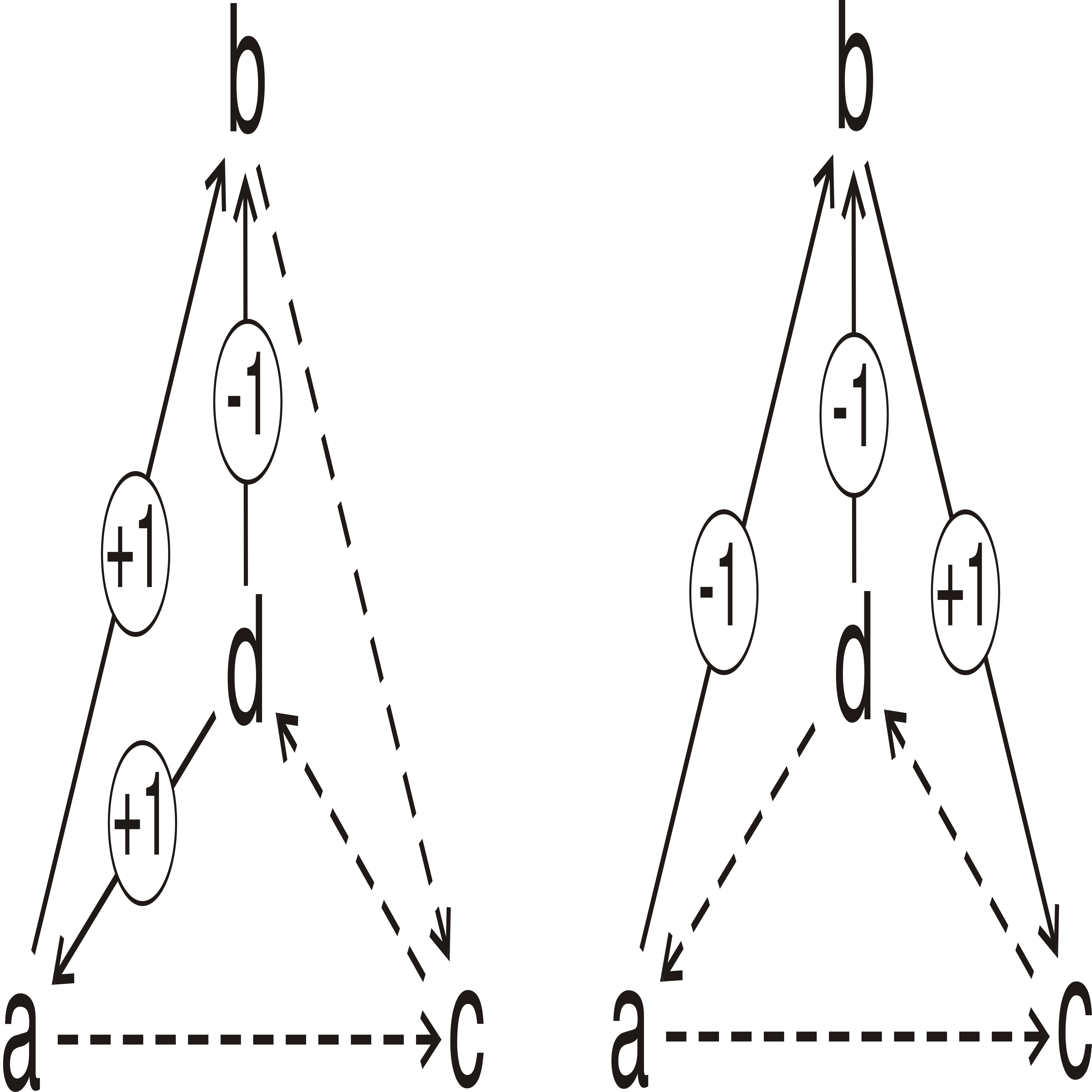
Figure 1: A basic cycle (on the left) and the basic cocycle $b^{\star}$ (on the right). A dashed edge indicates an edge-weight of zero.

Any fixed enumeration of the set $\overrightarrow{E}$ of edges of a tournament will identify each edge-weight assignment $\overrightarrow{w}$ with a point in the vector space $\mathbb{R}^{\frac{m(m-1)}{2}}$ (where $m=|\overrightarrow{V}|$) endowed with the standard inner product (for $\mathbf{u}=(u_{1},u_{2},\dots),$ $\mathbf{v}=(v_{1},v_{2},\dots)$, $\mathbf{u}\cdot\mathbf{v}=u_{1}v_{1}+u_{2}v_{2}+\dots$ – equivalently, multiply weights on corresponding edges, then add these products). With this identification, we obtain subspaces $\mathbf{V}\!_{\emph{cycle}}$ and $\mathbf{V}\!_{\emph{cocycle}}$ as the linear spans, respectively, of all basic cycles and of all basic cocycles.

For any tournament one can show that these two subspaces are orthogonal complements in $\mathbb{R}^{\frac{m(m-1)}{2}}$. Thus each vector $\overrightarrow{w}$ $\in\mathbb{R}^{\frac{m(m-1)}{2}}$ has a unique decomposition $\overrightarrow{w}=\overrightarrow{w}_{\emph{cycle}}+\overrightarrow{w}_{\emph{cocycle}}$ as a sum in which $\overrightarrow{w}_{\emph{cycle}}\in\mathbf{V}\!_{\emph{cycle}}$, $\overrightarrow{w}_{\emph{cocycle}}\in\mathbf{V}\!_{\emph{cocycle}}$, with $\overrightarrow{w}_{\emph{cycle}}\cdot\overrightarrow{w}_{\emph{cocycle}}=0$. See Examples 1 and 2 in this section; ? (?) provide detailed proofs and more examples. We say that $\overrightarrow{w}$ is purely cyclic if $\overrightarrow{w}=\overrightarrow{w}_{\emph{cycle}}$ (with $\overrightarrow{w}_{\emph{cocycle}}=\mathbf{0}$); $\overrightarrow{w}$ is purely acyclic if $\overrightarrow{w}=\overrightarrow{w}_{\emph{cocycle}}$ (with $\overrightarrow{w}_{\emph{cycle}}=\mathbf{0}$). A purely cyclic $\overrightarrow{w}$ always has majority cycles (unless it is the $\mathbf{0}$ vector), while a purely acyclic $\overrightarrow{w}$ never has any – in fact, purely acyclic weighted tournaments satisfy a strong, quantitative form of transitivity (see Definition 5).

Example 1

Consider a tournament on three vertices, with edges initially oriented cyclically: $a_{1}\rightarrow a_{2}\rightarrow a_{3}\rightarrow a_{1}$. The vector space of all edge-weight assignments is then $\mathbb{R}^{3}$; the cyclic subspace $\mathbf{V}\!_{\emph{cycle}}$ consists of all $\overrightarrow{w}$ that assign equal weights to these three edges, forming a one-dimensional line $L$ in $\mathbb{R}^{3}$ (passing through the points $(0,0,0)$ and $(1,1,1)$); and the cocyclic subspace $\mathbf{V}\!_{\emph{cocycle}}$ consists of all $\overrightarrow{w}$ that assign weights to these three edges that sum to $0$, forming a two-dimensional plane perpendicular to $L$.

Suppose the weight function $\overrightarrow{w}$ is of a mix of both components, with neither being zero. In this case, the weighted tournament may or may not exhibit a majority cycle – the situation depends on which component predominates in the sum. If the sign of $\overrightarrow{w}_{\emph{cycle}}+\overrightarrow{w}_{\emph{cocycle}}$ agrees with that of $\overrightarrow{w}_{\emph{cycle}}$ on enough edges, then $\overrightarrow{w}$ will exhibit a cycle, which we will refer to as “overt.” If not, then stripping out the cocyclic component will necessarily reveal a cycle, which had been masked or “hidden” by the cocyclic component. Thus, having no such hidden cycles is equivalent to pure acyclicity, and this condition is strictly stronger than having no overt cycles; for more on “hidden” versus “overt” cycles see Observation 1 and footnote 20.

In electrical engineering, this decomposition serves as the mathematical foundation of Kirchoff’s Laws (?, ) of circuit theory, but its roots lie in one-dimensional homology theory, within algebraic topology (see ?; ?; ?). In particular, the orthogonal projection of $\overrightarrow{w}$ onto $\mathbf{V}\!_{\emph{cocycle}}$ (which yields $\overrightarrow{w}_{\emph{cocycle}}$) coincides with the boundary map of homology. The decomposition was first applied to the flow of net preference by H. P. ? (?) in his characterization of Borda’s voting rule, and was later exploited by ? (?) and by ? (?). Quite recently, it was used by ? (?) to characterize the Mean Rule for the aggregation of dichotomous weak orders, and by ? (?) to characterize maximal lotteries. The relevance of the decomposition to profiles of weak or strict preference ballots can be appreciated from the following observation:

Observation 1

In the decomposition $\overrightarrow{w}=\overrightarrow{w}_{\emph{cycle}}+\overrightarrow{w}_{\emph{cocycle}}$ of any weight function $\overrightarrow{w}$ for a weighted tournament:

1. The cocyclic component $\overrightarrow{w}_{\emph{cocycle}}$ of $\overrightarrow{w}$ assigns to each edge $a\rightarrow b$ the scaled difference $\frac{a^{\beta}-b^{\beta}}{|\overrightarrow{V}|}$ in symmetric Borda scores of the two alternatives; we might say that “the Borda count is the boundary map.”

2. Thus, for a purely acyclic edge-weighting the pairwise majority relation yields a transitive ranking, which agrees with the ranking induced by Borda scores.

3. More generally, these two rankings agree when the cocyclic component is dominant in the sense that $\overrightarrow{w}(a,b)$ always agrees in sign with $\overrightarrow{w}_{\emph{cocycle}}(a,b)$. However, when the cyclic component becomes large enough to reverse a few edge weight signs, but not so many as to introduce Condorcet cycles (“overt” majority cycles), these rankings differ. That difference can be attributed to the “hidden” cycles of the cyclic component.

Example 2

Consider the following profile $\mathcal{T}_{28}$ with $28$ trichotomous weak order inputs on the four-element set $\{a,b,c,d\}$:

• 16 copies of $\{a\}>\{b,c\}>\{d\}$,

• 8 copies of $\{b\}>\{c\}>\{a,d\}$,

• 4 copies of $\{b,c\}>\{d\}>\{a\}$.

The induced weighted tournament is on the left of Figure 2; its weight function $\overrightarrow{w}$ is a vector in $\Re^{6}$. To see why the weight on the $d\rightarrow a$ edge is $-12$ (for example), note that the first $16$ orders have $a>d$, the next $8$ have $a\sim d$ and the last $4$ have $d>a$, for a resulting “net preference for $d$ over $a$” of $-16+0+4=-12$.

Symmetric Borda scores for $\mathcal{T}_{28}$ are $a^{\beta}=20$, $b^{\beta}=32$, $c^{\beta}=16$, and $d^{\beta}=-68$ (see footnote 12). As $|\overrightarrow{V}|=4$, $\frac{a^{\beta}-b^{\beta}}{|\overrightarrow{V}|}=-3=\overrightarrow{w}_{\emph{cocycle}}(a,b)$, whence (by Observation 1.1) the $a\rightarrow b$ edge – for example – of the middle tournament is labeled $-3$ in Figure 2. Edge-weights for $\overrightarrow{w}_{\emph{cycle}}$ are then determined by $\overrightarrow{w}_{\emph{cycle}}(x,y)=\overrightarrow{w}(x,y)-\overrightarrow{w}_{\emph{cocycle}}(x,y)$.

The cocyclic component may now be written as the linear combination

$$5a^{\star}+8b^{\star}+4c^{\star}-17d^{\star}$$

of all four basic cocycles, in which the coefficient of $x^{\star}$ is $\frac{x^{\beta}}{|\overrightarrow{V}|}$; alternately one can use $a^{\star}+b^{\star}+c^{\star}+d^{\star}=\mathbf{0}$ to express $\overrightarrow{w}_{\emph{cocycle}}$ in terms of any three basic cocycles. As shown in Figure 3, $\overrightarrow{w}_{\emph{cycle}}$ can be written as a linear combination

$$7(a\rightarrow b\rightarrow d\rightarrow a)+4(b\rightarrow c\rightarrow d\rightarrow b)+3(a\rightarrow c\rightarrow d\rightarrow a)$$

of three basic cycles. The $-3$ on the $d\rightarrow b$ edge of $\overrightarrow{w}_{\emph{cycle}}$ can then be seen as the sum of $+4$ from $4(b\rightarrow c\rightarrow d\rightarrow b)$ and $-7$ from $7(a\rightarrow b\rightarrow d\rightarrow a)$ (negative because the sense of the cycle opposes that of the directed edge).

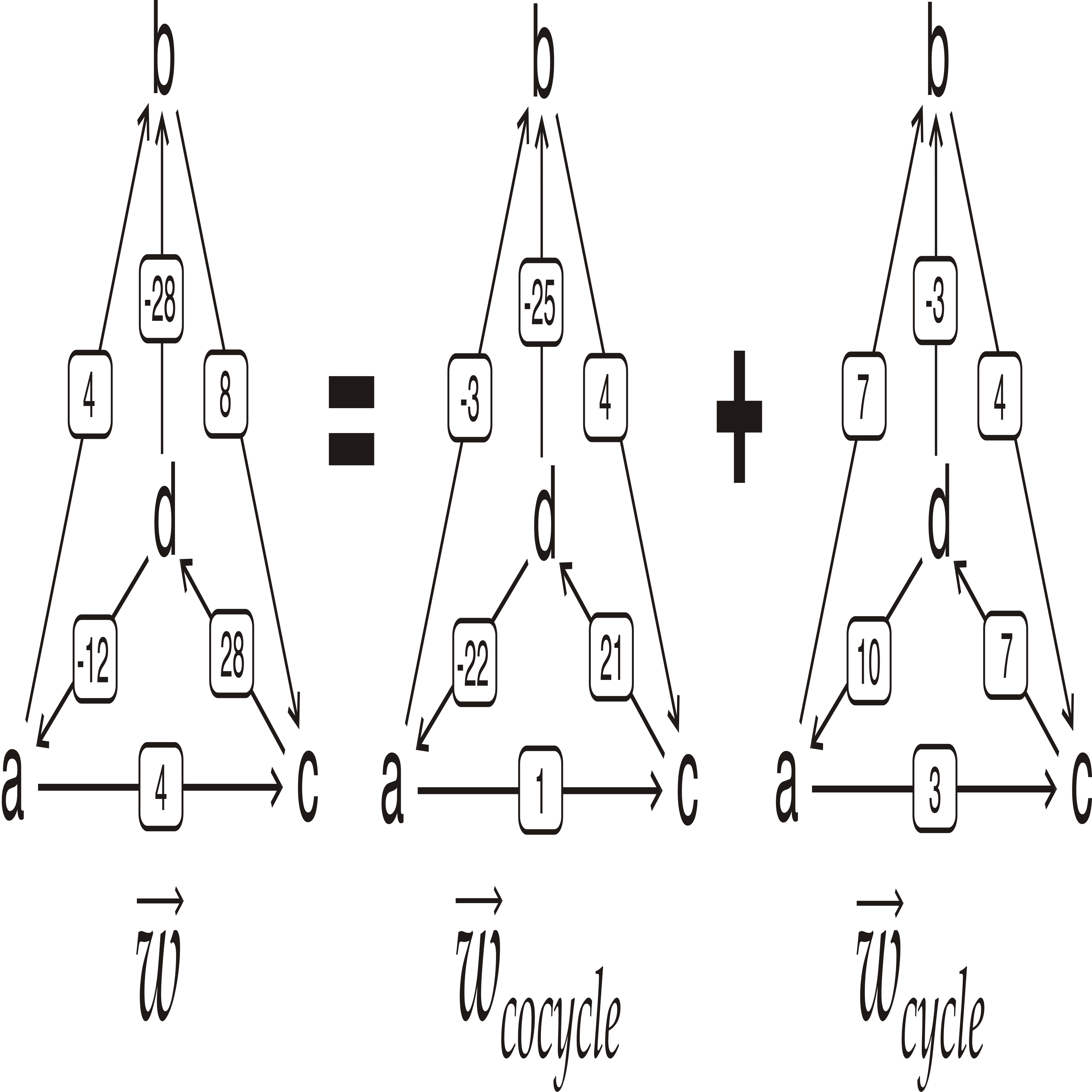
Figure 2: The weighted tournament induced by profile $\mathcal{T}_{28}$, and its decomposition.

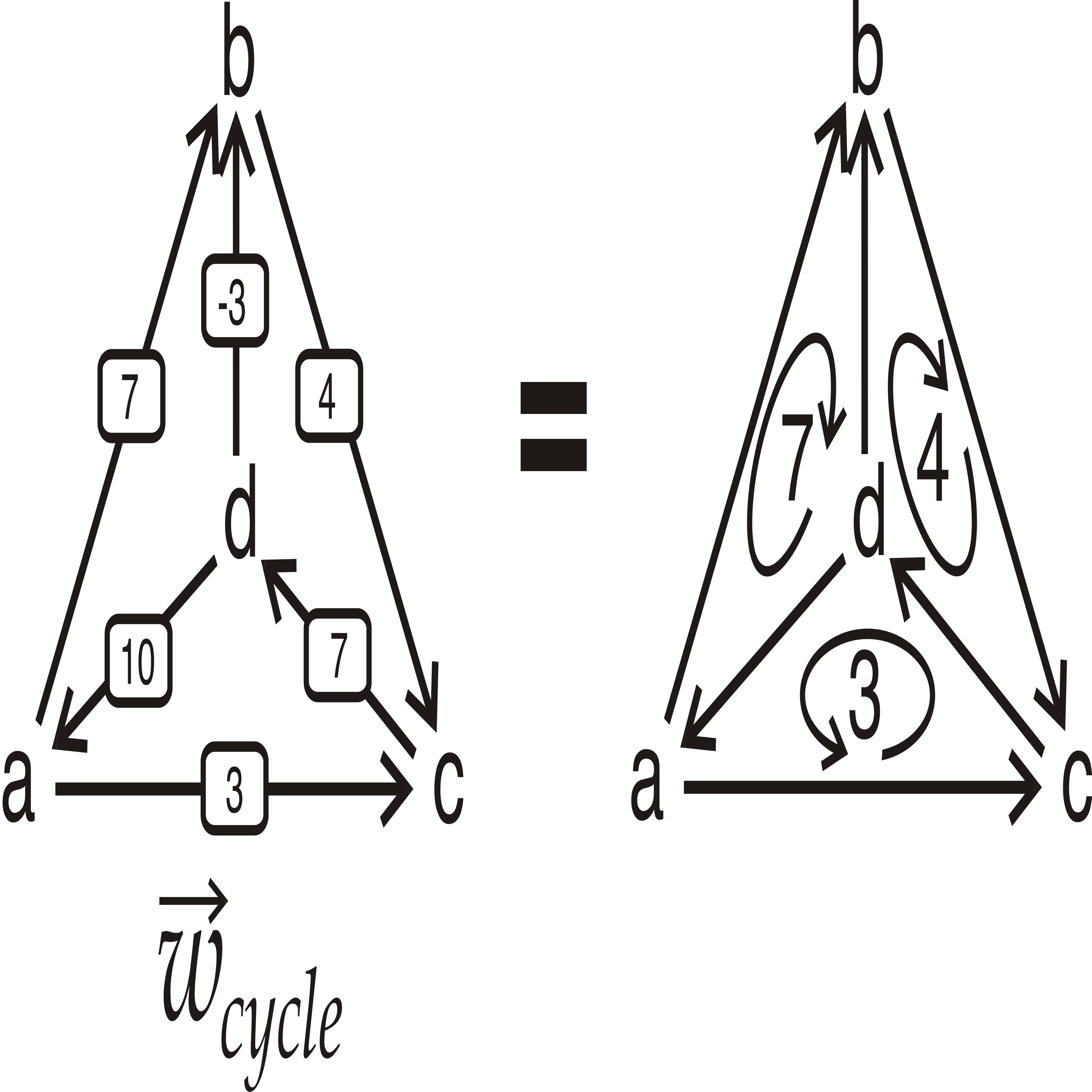
Figure 3: The cyclic component from Figure 2 written as a linear combination of three basic cycles.

4 A Version of Max Cut for Weighted Tournaments

In the well known max cut problem, one starts with an undirected graph $\mathcal{G}=(V,E)$ with finite vertex set $V$. A vertex cut is a partition $\mathcal{P}=\{J,K\}$ of $V$ into two pieces, and is assigned a score $v(\mathcal{P})$ equal to the number of edges $\{a,b\}\in E$ whose vertices are “cut” by $\mathcal{P}$ (meaning $a\in J$ and $b\in K$, or $a\in K$ and $b\in J$). The max cut (decision) problem takes $\mathcal{G}$ along with a positive integer $s$ as input, and asks whether there exists a vertex cut of $\mathcal{G}$ with score at least $s$. It is one of the best known $\mathit{NP}$-complete problems. The corresponding optimization problem seeks a cut of maximal score; any such optimization problem inherits $\mathit{NP}$-hardness when the associated decision problem is $\mathit{NP}$-hard.

For our purposes, a certain generalization will be useful. A vertex $k$-partition $\mathcal{P}$ has $k$ nonempty pieces, with score equal to the number of edges $\{a,b\}\in E$ whose vertices belong to different pieces of $\mathcal{P}$. The max $k$-cut problem then asks whether there exists any $k$-partition meeting or exceeding some specified threshold score, with corresponding optimization problem formulated as one would expect. Our main concern will be with the weighted versions of these problems: in a weighted graph $\mathcal{G}=(V,E,w)$ the function $w$ assigns an edge-weight $w(e)\geq 0$ to each edge $e\in E$ and the score is the sum of the weights assigned to edges that are cut. The decision problem (or optimization problem) is similarly $\mathit{NP}$-complete (respectively, $\mathit{NP}$-hard). For the weighted version there is no loss of generality in assuming $\mathcal{G}$ is complete; just add all the missing edges and assign them weight zero.

We consider a version of max cut for weighted tournaments or directed graphs $\overrightarrow{\mathcal{H}}=(\overrightarrow{V},\overrightarrow{E},\overrightarrow{w})$ for which the real-number edge-weights may be negative, with a linearly ordered partition of the vertices playing the role of a “cut.” For example, we might partition $\overrightarrow{V}$ into two disjoint and nonempty pieces, $T$ (for top) and $B$ (for bottom); the ordered partition $\overrightarrow{\mathcal{P}}=\{T>B\}$ is then equivalent to a dichotomous weak order $\succeq$ on $\overrightarrow{V}$. An ordered tripartition $\{T>M>B\}$ similarly corresponds to a trichotomous weak order on $\overrightarrow{V}$, while a linear order on $V$ is equivalent to an ordered $|\overrightarrow{V}|$-partition, which has as many non-empty pieces as there are vertices, so that each piece is a singleton.

Given a weighted tournament $\overrightarrow{\mathcal{H}}=(\overrightarrow{V},\overrightarrow{E},\overrightarrow{w})$ and an ordered $k$-partition $\overrightarrow{\mathcal{P}}$ corresponding to a $k$-chotomous weak order $\succeq$ on $\overrightarrow{V}$, we say that an edge $(x,y)$ goes down if $x\succ y$, goes up if $y\succ x$, and goes sideways if $x\sim y$. For the example in Figure 4, $(a,c)$, $(a,e)$ and $(d,f)$ go down; $(g,b)$, $(g,d)$ and $(c,b)$ go up; and $(a,b)$ and $(f,e)$ go sideways. The score $\overrightarrow{v}$ of an ordered $k$-partition $\overrightarrow{\mathcal{P}}$ is now defined from the original (not extended) $\overrightarrow{w}$ by:

$$\overrightarrow{v}\!_{\overrightarrow{w}}(\overrightarrow{\mathcal{P}})=\sum_{(x,y)\in\overrightarrow{E}\;\emph{goes down}}\overrightarrow{w}(x,y)\hskip 14.22636pt-\sum_{(u,v)\in\overrightarrow{E}\;\emph{goes up}}\overrightarrow{w}(u,v).$$ (2)

Note that the score is independent of weights on sideways edges. Thus in Figure 4 we have

$$\overrightarrow{v}\!_{\overrightarrow{w}}(\overrightarrow{\mathcal{P}})=[3+4+5]-[1+3+4]=4.$$ (3)

Figure 4: A weighted directed graph and ordered $3$-partition

If we instead interpret $\overrightarrow{w}$ as denoting the antisymmetric extension of the original weight function (see Section 2), equation (2) can be rewritten as:

$$\overrightarrow{v}\!_{\overrightarrow{w}}(\overrightarrow{\mathcal{P}})=\sum_{x\,\succ\,y}\overrightarrow{w}(x,y).$$ (4)

Definition 2

Max $k$-OP (“OP” for “ordered partition”) is the decision problem that takes as input a weighted tournament $\overrightarrow{\mathcal{H}}=(\overrightarrow{V},\overrightarrow{E},\overrightarrow{w})$ for which $\overrightarrow{w}$ is integer-valued, along with an integer $s$, and asks whether there exists an ordered $k$-partition with score at least $s$. The corresponding optimization problem seeks an ordered partition achieving maximal score.

Why propose this particular adaptation of max cut for tournaments? For one thing, max $k$-OP serves as the basis for a generalization (in Section 5) of the Kemeny voting rule that yields a variety of aggregation rules – rules already known to social choice and judgement aggregation – as special cases. A second justification arises from mathematical naturality; solving max $k$-OP is equivalent to finding a vector (from among those representing $k$-chotomous weak orders) that maximizes the inner product with a given, second vector (representing the weight function $\overrightarrow{w}$). The equivalence will be discussed by ? (?).

Our goal is to show that both the purely cyclic and the transitive subcases of max $k$-OP are $\mathit{NP}$-complete for $k\geq 3$, but polynomial-time solvable for $k=2$ and for arbitrary $k$ when $\overrightarrow{w}_{\emph{cycle}}=\mathbf{0}$. A first hardness result reduces max $3$-cut to the purely cyclic sub-case of max $3$-OP, while a second construction reduces max $2$-cut to the transitive sub-case of max $3$-OP. Either reduction alone suffices to show that max $3$-OP is $\mathit{NP}$-complete (as max $3$-OP is easily seen to lie in $\mathit{NP}$), but the two serve different roles. The first establishes that intractability can arise from the cyclic component in isolation – a mix of both components is not required. However, it leaves open the possibility that overt majority cycles alone suffice for the analysis, with no role left for the orthogonal decomposition and its revelation of hidden cycles in explaining why some instances of max $k$-OP are in $P$ while others are $\mathit{NP}$-hard. By showing that the transitive subcase remains $\mathit{NP}$-hard, the second reduction closes off this possibility and (in light of the first easiness result) establishes the essential role of hidden cycles in explaining the hardness boundary in max $3$-OP.

Theorem 1

Let $k\geq 3$.

1. The problem max $k$-OP is $\mathit{NP}$-complete, even in the purely cyclic case.

2. The problem max $k$-OP is $\mathit{NP}$-complete, even in the transitive case.

Our first easiness result shows that the purely acyclic sub-case of max $k$-OP is solvable in polynomial time, for each $k\geq 2$. The second result shows that for the special case $k=2$, the cyclic component has no effect on the the solution to max $k$-OP; we may safely suppress it, at which point the first easiness result applies.

Theorem 2

The following problems are polynomial-time solvable:

1. the purely acyclic case of max $k$-OP (for each fixed $k\geq 2$, and also with $k$ folded in to the input),

2. max $2$-OP.

In combination these two theorems argue that the two components have independent effects on computational complexity.

If we attacked max $k$-OP via brute force search over all ordered $k$-partitions (of the vertex set $\overrightarrow{V}$ of a weighted tournament), then for any fixed $k\geq 2$ we would find that the number of such partitions grows exponentially in the number $|\overrightarrow{V}|$ of vertices. The key idea in the proof of Theorem 2.1 is that this search space can be reduced to one of polynomial size $\mathcal{O}(|\overrightarrow{V}|^{k-1})$ for fixed $k$ and purely acyclic $\overrightarrow{w}$; part 2 follows from part 1, once we show that the cyclic component may be ignored for the special case of ordered partitions into exactly two pieces.

We turn now to the proof of Theorem 1.1, beginning with a polynomial reduction of max $3$-cut to max $3$-OP. The idea is to replace a weighted graph $\mathcal{G}$ with a correspondingly weighted tournament $\overrightarrow{\mathcal{H}_{\mathcal{G}}}$ in such a way that each tripartition $\mathcal{P}$ of $\mathcal{G}$’s vertices corresponds to an ordered tripartition $\overrightarrow{\mathcal{P}}$ of $\overrightarrow{\mathcal{H}_{\mathcal{G}}}$’s vertices satisfying $v(\mathcal{P})=\overrightarrow{v}(\overrightarrow{\mathcal{P}})$. The $\overrightarrow{\mathcal{H}_{\mathcal{G}}}$ construction produces, for each edge $\{a,b\}$ of $\mathcal{G}$, two new vertices (in addition to the original vertices of $\mathcal{G}$) and four edges. More precisely:

Definition 3

Let $\mathcal{G}=(V,E)$ be any complete (finite, undirected) graph and $w\!:\!E\rightarrow\mathbb{R}$ be an associated nonnegative edge-weight function. The induced weighted tournament $\overrightarrow{\mathcal{H}_{\mathcal{G}}}$ is defined as follows:

• For each edge $e=\{a,b\}\in E$ of $\mathcal{G}$, construct two direction vertices $d_{ab}$ and $d_{ba}$ of $\mathcal{H}_{\mathcal{G}}$. Let $D=\{d_{ab}\;|\;\{a,b\}\in E\}$ denote the set of direction vertices and assume $D\cap V=\emptyset$.

• $\overrightarrow{\mathcal{H}_{\mathcal{G}}}$’s vertex set is $\overrightarrow{V}=D\cup V$, with elements of $V$ referred to as ordinary vertices.

• Add all edges of form $a\rightarrow d_{ab}$ and $d_{ab}\rightarrow b$ to $\overrightarrow{\mathcal{H}_{\mathcal{G}}}$, with $\overrightarrow{w}$ assigning to each the original weight $w(\{a,b\})$ of $\{a,b\}$ in $\mathcal{G}$; then add enough arbitrarily directed edges to make $\overrightarrow{\mathcal{H}_{\mathcal{G}}}$ a tournament, with $\overrightarrow{w}$ assigning weight $0$ to each of these.

Notice that each edge $e=\{a,b\}$ of $\mathcal{G}$ thus contributes an $\{a,b\}$ $4$-cycle

$$a\longrightarrow d_{ab}\longrightarrow b\longrightarrow d_{ba}\longrightarrow a$$ (5)

of edges in $\overrightarrow{\mathcal{H}_{\mathcal{G}}}$, each with weight $w(\{a,b\})$. In particular, $\overrightarrow{w}$ is purely cyclic. The combinatorial core of the Theorem 1.1 proof consists of the following:

Lemma 1

(Fitting a four-cycle into three levels) Let $\overrightarrow{\mathcal{P}}=\{T>M>B\}$ be any ordered tripartition of the vertex set $\overrightarrow{V}$ of $\overrightarrow{\mathcal{H}_{\mathcal{G}}}$. Then for each weight $w$ edge $e=\{a,b\}$ of $\mathcal{G}$:

• if $a$ and $b$ belong to the same piece of $\overrightarrow{\mathcal{P}}$ then the net contribution to the score $\overrightarrow{v}(\overrightarrow{\mathcal{P}})$ made by the edges of the $\{a,b\}$ $4$-cycle of line (5) is zero, and

• if $a$ and $b$ belong to any two different pieces of $\overrightarrow{\mathcal{P}}$ then, by appropriately reassigning the direction vertices $d_{ab}$ and $d_{ba}$ among $T$, $M$, and $B$, we can set the net contribution to $\overrightarrow{v}(\overrightarrow{\mathcal{P}})$ made by the edges of the $\{a,b\}$ $4$-cycle equal to $0$, or $+w$, or $-w$, as we prefer.

Proof: Figures 5L, 5C, and 5R (for Left, Center, Right) show three possible ways to assign the four vertices $a,b,d_{ab}$ and $d_{ba}$ to membership in the three pieces of $\overrightarrow{\mathcal{P}}$. In 5R ordinary vertices $a$ and $b$ belong to the same piece (here, piece $M$) of $\overrightarrow{\mathcal{P}}$. Of the four edges in the $\{a,b\}$ 4-cycle, two are up edges and two are down edges; as each edge has weight $w$ the net contribution of these four edges is zero. More generally, whenever $a,b\in M$ it is easy to see that the number of up edges from the $\{a,b\}$ 4-cycle must equal the number of down edges, no matter where $d_{ab}$ and $d_{ba}$ are placed, and that this remains true in case $a,b\in T$ or $a,b\in B$. Thus the net contribution is $0$ whenever the ordinary vertices $a$ and $b$ are in the same piece.

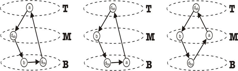
Figure 5: Some possible ways to fit an $\{a,b\}$ $4$-cycle into three levels.

In 5L and 5C, ordinary vertices $a$ and $b$ are in different pieces, and we have placed $d_{ab}$ and $d_{ba}$ so that there are two down edges and one up edge. If each edge has weight $w$ then the net contribution of the four edges shown is $w$. If we exchange the placements of $d_{ab}$ and $d_{ba}$ in 5L (or in 5C), we wind up with two up edges and one down edge for a net contribution of $-w$; if we move $d_{ab}$ and $d_{ba}$ into a common piece, then (as in the previous paragraph) the number of up edges will be equal to the number of down edges, for a net contribution of zero. A moment’s thought will convince the reader that for all cases in which ordinary vertices $a$ and $b$ belong to different pieces, exactly four possibilities – two up edges and one down, two down edges and one up, one down edge and one up, or two down edges and two up – can be achieved by moving $d_{ab}$ and $d_{ba}$ around. This completes the Lemma 1 proof.  

We are now ready to prove Theorem 1, parts 1 and 2.

Proof of Theorem 1.1: Continuing, for the moment, with the special case $k=3$, it suffices to show that given an edge-weighted graph $\mathcal{G}$ and a positive integer $r$ the answer to the decision problem “Does there exist a vertex tripartition $\mathcal{P}=\{J,K,L\}$ of $V$ with $v(\mathcal{P})\geq r$?” is the same as the answer to “Does there exist an ordered tripartition $\overrightarrow{\mathcal{P}}$ of the vertex set $\overrightarrow{V}$ of $\overrightarrow{\mathcal{H}_{\mathcal{G}}}$ with $\overrightarrow{v}(\overrightarrow{\mathcal{P}})\geq r$?”

Lemma 1 makes this easy. Given a tripartition $\mathcal{P}=\{J,K,L\}$ of $V$ with $v(\mathcal{P})=q\geq r$, arbitrarily order $\{J,K,L\}$ as $\{J>K>L\}$, which becomes the ordered partition of $\overrightarrow{\mathcal{H}_{\mathcal{G}}}$’s ordinary vertices. For each weight $w$ edge $\{a,b\}$ of $\mathcal{G}$ cut by $\mathcal{P}$, add each direction vertex $d_{ab}$, $d_{ba}$ to one of the sets in $\{J>K>L\}$, so as to create two down edges and one up edge from the $\{a,b\}$ 4-cycle; for each original uncut edge $\{a,b\}$ of $\mathcal{G}$ add each vertex $d_{ab}$, $d_{ba}$ to one of the sets $\{J>K>L\}$ arbitrarily. It is easy to see that the resulting $\overrightarrow{\mathcal{P}}$ achieves the exact same score: $\overrightarrow{v}(\overrightarrow{\mathcal{P}})=v(\mathcal{P})=q\geq r.$

In the other direction, consider an ordered tripartition $\overrightarrow{\mathcal{P}}=\{V_{1}\cup D_{1}>V_{2}\cup D_{2}>V_{3}\cup D_{3}\}$ of $\overrightarrow{V}$ with $V_{1}\cup V_{2}\cup V_{3}=V$, $D_{1}\cup D_{2}\cup D_{3}=D$, and $\overrightarrow{v}(\overrightarrow{\mathcal{P}})\geq r$. Let $\mathcal{P}=\{V_{1},V_{2},V_{3}\}$, a tripartition of $V$. Each weight $w$ edge $\{a,b\}$ of $\mathcal{G}$ cut by $\mathcal{P}$ contributes $w$ to $v(\mathcal{P})$ and contributes $w$ or $0$ or $-w$ to $\overrightarrow{v}(\overrightarrow{\mathcal{P}})$. Thus $v(\mathcal{P})\geq\overrightarrow{v}(\overrightarrow{\mathcal{P}})\geq r$, as desired. This completes our polynomial reduction of max $3$-cut to max $3$-OP.

Our argument generalizes easily to a polynomial reduction of max $k$-cut to max $k$-OP; in particular, the construction of $\overrightarrow{\mathcal{H}_{\mathcal{G}}}$ does not change at all, while the proof of Lemma 1 generalizes straightforwardly for ordered partitions into $k\geq 3$ pieces.

We will combine this reduction with the following straightforward reduction of max cut to max $k$-cut: to a weighted graph add $k-2$ new vertices, along with new edges joining them to each other and to all old vertices, and place very large weights on all these new edges. A maximal-score partition $\mathcal{P}^{\dagger}$ of the enlarged weighted graph then consists of any maximal score partition $\mathcal{P}$ of the original vertices into two pieces, combined with $k-2$ other sets, each containing one new vertex. Thus $\mathcal{P}$ may be read off from $\mathcal{P}^{\dagger}$.

The combination reduces max cut to (the purely cyclic case of) max $k$-OP, for each $k\geq 3$. As max cut is known to be $\mathit{NP}$-complete, while max $k$-OP (along with its purely cyclic sub-case) is clearly in class $\mathit{NP}$, Theorem 1.1 now follows.  

We turn now to the proof of Theorem 1.2, which reduces max cut to the transitive sub-case of max $k$-OP. Transitivity here refers to the ordinary “qualitative” version, as expressed for a weighted tournament $\overrightarrow{\mathcal{H}}=(\overrightarrow{V},\overrightarrow{E},\overrightarrow{w})$, by:

$$\emph{If }\overrightarrow{w}(x,y)>0\emph{ and }\overrightarrow{w}(y,z)>0\emph{ then }\overrightarrow{w}(x,z)>0,$$ (6)

for all $x,y\in V$ with $x\neq y$ (with $\overrightarrow{w}$ denoting the antisymmetric extension of Section 2).

Proof of Theorem 1.2: Transitive max $3$-OP reduces to transitive max $k$-OP for any (finite) $k\geq 4$, as follows: add $k-3$ new vertices $D_{1},\dots,D_{k-3}$ and put very large weights on all $x\rightarrow D_{j}$ edges for $x\in V$ and all $D_{i}\rightarrow D_{j}$ edges for $i<j$, so that any optimal ordered partition consists of an optimal ordered partition of the original vertices into three pieces, sitting above $k-3$ additional pieces, each of form $\{D_{j}\}$. It suffices, then, to reduce max cut to transitive max $3$-OP.

As in the proof of Theorem 1.1, we specify a polynomial translation that converts a weighted graph $\mathcal{G}=(V,E,w)$ containing $|V|$ vertices (which – without loss of generality – is complete and for which $w(e)$ is a nonnegative integer for each edge $e=\{a,b\}\in E$) into a weighted tournament $\overrightarrow{\mathcal{F}_{\mathcal{G}}}=(\overrightarrow{V},\overrightarrow{E},\overrightarrow{w})$. This time our goals for $\overrightarrow{\mathcal{F}_{\mathcal{G}}}$ are a bit different. Let $C=1+\Sigma_{e\in E}w(e)$ and $\varepsilon=\frac{1}{72|V|^{4}}$. Then our construction will satisfy that:

1. $\overrightarrow{w}$ is transitive in the sense of equation (6), and

2. For each positive integer $r$ the answer to the decision problem “Does there exist a vertex bipartition $\mathcal{P}=\{J,K\}$ of $V$ with $v(\mathcal{P})\geq r$?” is the same as the answer to “Does there exist an ordered tripartition $\overrightarrow{\mathcal{P}}$ of the vertex set $\overrightarrow{V}$ of $\overrightarrow{\mathcal{F}_{\mathcal{G}}}$ with

   $$\overrightarrow{v}(\overrightarrow{\mathcal{P}})\geq\langle\!\langle 3|V|C+r\rangle\!\rangle?"$$ (7)

Here $\langle\!\langle x\rangle\!\rangle$ rounds $x$ to the nearest integer. Given $\mathcal{G}=(V,E)$ and $w\!\!:\!E\rightarrow\Re$ as above, we now define the weighted tournament $\overrightarrow{\mathcal{F}_{\mathcal{G}}}=(\overrightarrow{V},\overrightarrow{E},\overrightarrow{w})$ induced by $\mathcal{G}$ and $w$ as follows:

• Choose any reference linear order $\triangleright$ of $\mathcal{G}$’s vertex set $V$.

• Each vertex $a\in V$ contributes a quadruple of ordinary vertices $a_{1},a_{2},a_{3}$, and $a_{4}$ to $\overrightarrow{V},$ along with three directed “placement” edges (see Figure 6):

  $$a_{1}\longrightarrow a_{2}\longrightarrow a_{3}\longrightarrow a_{4}$$ (8)

  weighted as follows: $\overrightarrow{w}(a_{2},a_{3})=2C$ and $\overrightarrow{w}(a_{1},a_{2})=C=\overrightarrow{w}(a_{3},a_{4})$.

• Each edge $e=\{a,b\}$ of $\mathcal{G}$ having weight $w$ and satisfying $a\,\triangleright\,b$ contributes two additional direction vertices $d_{ab}$ and $d_{ba}$ to $\overrightarrow{V}$, along with four directed “adjustment” edges:

  $$a_{2}\longrightarrow d_{ab}\longrightarrow b_{2}\emph{; }\,\,b_{3}\longrightarrow d_{ba}\longrightarrow a_{3}$$ (9)

  with each such edge assigned weight $w$ (if $w>0$) or weight $\varepsilon$ (if $w=0$).

• To make $\overrightarrow{\mathcal{F}_{\mathcal{G}}}$ into a tournament, we need to add edges between pairs of vertices that are not yet linked in either direction. The direction of each can be chosen carefully (as detailed immediately below) in such a way that no cycles are created. Assign weight $\varepsilon$ to each of these “tiny” edges.

Suppose we temporarily erase all weights on the edges of $\overrightarrow{\mathcal{F}_{\mathcal{G}}}$, and also omit all the tiny edges, retaining the placement and adjustment edges. The resulting unweighted digraph $\mathcal{E}_{\mathcal{G}}$ is acyclic (meaning there are no cycles that respect edge direction), thanks to the use of the reference linear order $\triangleright$; staring at Figure 6 can help explain what’s going on here. Any such acyclic digraph can be extended to an acyclic tournament by adding new edges one-at-a-time. Once these tiny edges are added and assigned positive weight $\varepsilon$, the resulting weighted tournament is transitive, as desired. Moreover, $\varepsilon$ is small enough to guarantee that the total contribution of all weight $\varepsilon$ edges to the score of any ordered tripartition is less than $\frac{1}{2}$ in absolute value. Thus we are safe when, for the remainder of this proof, we simultaneously ignore the presence of weight $\varepsilon$ edges and use of rounding in condition 7.

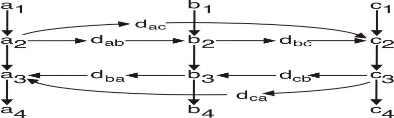
Figure 6: Part of the digraph $\mathcal{E}_{\mathcal{G}}$ showing the (directed) placement and adjustment edges arising from three vertices $a\triangleright b\triangleright c$ (and corresponding undirected edges) of $\mathcal{G}$. Note the absence of cycles.

Any score-maximizing tripartition $\overrightarrow{\mathcal{P}}=\{T>M>B\}$ of $\overrightarrow{\mathcal{F}_{\mathcal{G}}}$ will also maximize that part of the score contributed by the placement edges (which have weight $2C$ or weight $C$), because the value of $C$ is large enough to make any nonzero contribution by a single weight-$C$ edge overwhelm the total contribution of all adjustment edges (which have weights from the original graph $\mathcal{G}$). To maximize the placement edge part of the score it is necessary, for each quadruple $a_{1},a_{2},a_{3},a_{4}$ of ordinary vertices, either to place $a_{1},a_{2}\in T$, $a_{3}\in M$, and $a_{4}\in B$ – in which case we will say that $\overrightarrow{\mathcal{P}}$ places $a$ up – or $a_{1}\in T$, $a_{2}\in M$, and $a_{3},a_{4}\in B$ – in which case $\overrightarrow{\mathcal{P}}$ places $a$ down. Either such arrangement achieves a contribution of $3C$ from $a_{1},a_{2},a_{3},a_{4}$, and it is easy to see that one cannot do better than that. Hence, when seeking to maximize the score of $\overrightarrow{\mathcal{P}}$ we may assume that each original vertex of $\mathcal{G}$ is either placed up or down, for a total contribution of $3|V|C$ from placement edges.

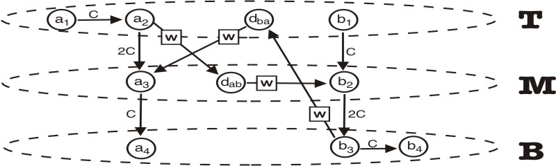
Figure 7: Two quadruples (with $a$ up, $b$ down) and direction vertices (as positioned to achieve a net contribution of $w$ from the adjustment edges).

Assume the weight of some edge $\{a,b\}$ of $\mathcal{G}$ is $w$, and $a\triangleright b$. Figure 5 shows the corresponding quadruples, placed in an ordered $3$-partition $\overrightarrow{\mathcal{P}}$ so that $a$ is up and $b$ down. The direction vertices $d_{ab}$ and $d_{ba}$ have been positioned so that the net contribution made to $\overrightarrow{v}(\overrightarrow{\mathcal{P}})$ by the four corresponding adjustment edges is $w+0-w+w=w$. It is straightforward to check that one cannot achieve a contribution greater than $w$ by moving $d_{ab}$ and $d_{ba}$ into different pieces of $\overrightarrow{\mathcal{P}}$. The situation is the same when $a$ is down and $b$ is up; one can position $d_{ab}$ and $d_{ba}$ to achieve a net contribution of $w$ from the adjustment edges, and no greater contribution is possible. Finally, when $a$ and $b$ are either both up, or both down, the net contribution made by the four corresponding adjustment edges is $0$, regardless of where one positions $d_{ab}$ and $d_{ba}$.

Thus, given a partition $\mathcal{P}=\{U,D\}$ of $\mathcal{G}$’s vertices with a score $v(\mathcal{P})$ of at least $r$ one can construct an ordered $3$-partition $\overrightarrow{\mathcal{P}}$ of $\overrightarrow{\mathcal{F}_{\mathcal{G}}}$’s vertices with score at least $3|V|C+r$ by placing all vertices in $U$ up, all in $D$ down, and positioning the direction vertices to maximize the contribution of adjustment edges, as detailed in the previous paragraph. Conversely, given an ordered $3$-partition $\overrightarrow{\mathcal{P}}$ of $\overrightarrow{\mathcal{F}_{\mathcal{G}}}$’s vertices with score at least $3|V|C+r$, we know that each original vertex must be placed in the up or down position. The considerations of the previous paragraph then imply that by setting $U=\{a\in V\,|\,a\emph{ is up}\}$ and $V=\{b\in V\,|\,b\emph{ is down}\}$ we obtain a partition $\{U,V\}$ of $\mathcal{G}$’s vertices with a score of at least $r$.  

The proof of Theorem 2 rests on a sequence of lemmas and definitions, including the abstract definition of Borda score as the “net weighted out-degree” of a vertex $x$ in a weighted tournament. In the following definitions $\overrightarrow{w}$ denotes the antisymmetric extension, as discussed in Section 2.

Definition 4

Given a vertex $x$ of a weighted tournament $\overrightarrow{\mathcal{H}}=(\overrightarrow{V},\overrightarrow{E},\overrightarrow{w})$, $x$’s Borda score is given by:

$$x^{\beta}=\sum_{y\,\in V}\overrightarrow{w}(x,y)$$ (10)

Definition 5

A weighted tournament $\overrightarrow{\mathcal{H}}=(\overrightarrow{V},\overrightarrow{E},\overrightarrow{w})$ satisfies exact quantitative transitivity if

$$\overrightarrow{w}(x,y)+\overrightarrow{w}(y,z)=\overrightarrow{w}(x,z)$$ (11)

holds for every three distinct vertices $x,y,z\in\overrightarrow{V}$.

Definition 6

A weighted tournament $\overrightarrow{\mathcal{H}}=(\overrightarrow{V},\overrightarrow{E},\overrightarrow{w})$ is difference generated if there exists a function $\Gamma\!\!:\overrightarrow{V}\rightarrow\mathbb{R}$ such that

$$\overrightarrow{w}(x,y)=\Gamma(x)-\Gamma(y)$$ (12)

holds for every two distinct vertices $x,y\in\overrightarrow{V}$. In this case, we can identify the vertices of $\overrightarrow{\mathcal{H}}$ with a sequence of real numbers

$$\gamma_{1}\leq\gamma_{2}\leq\dots\leq\gamma_{m}$$ (13)

enumerating $\Gamma$’s values in non-decreasing order.

We show next that pure acyclicity is equivalent to difference generated-ness as well as to quantitative transitivity:

Lemma 2

The following are equivalent for a weighted tournament $\overrightarrow{\mathcal{H}}=(\overrightarrow{V},\overrightarrow{E},\overrightarrow{w})$:

1. $\overrightarrow{w}$ satisfies exact quantitative transitivity,

2. $\overrightarrow{w}$ is difference generated,

3. $\overrightarrow{w}$ is purely acyclic (equivalently, $w_{\emph{cycle}}=\mathbf{0}$ in the vector orthogonal decomposition $\overrightarrow{w}=\overrightarrow{w}_{\emph{cycle}}+\overrightarrow{w}_{\emph{cocycle}}$; equivalently, $\overrightarrow{w}\in\mathbf{V}_{\emph{cocycle}}$, the cocycle subspace).

Proof of Lemma 2: For $(1)\Rightarrow(2)$, assume $\overrightarrow{w}$ satisfies exact quantitative transitivity. Choose any $x_{0}\in\overrightarrow{V}$, and assign an arbitrary real number (a discrete analogue of a constant of integration) as $\Gamma(x_{0})$’s value. For each $y\in\overrightarrow{V}$ set $\Gamma(y)=\overrightarrow{w}(y,x)+\Gamma(x_{0})$. Then for $y,z\in\overrightarrow{V},$ $\overrightarrow{w}(y,z)=\overrightarrow{w}(y,x)+\overrightarrow{w}(x,z)=\overrightarrow{w}(y,x)-\overrightarrow{w}(z,x)=[\hskip 0.56905pt\overrightarrow{w}(y,x)+\Gamma(x_{0})]-[\hskip 0.56905pt\overrightarrow{w}(z,x)+\Gamma(x_{0})]=\Gamma(y)-\Gamma(z)$. Conversely, if $\overrightarrow{w}$ is difference generated via $\Gamma$ then $\overrightarrow{w}(y,x)+\overrightarrow{w}(x,z)=[\hskip 0.56905pt\Gamma(y)-\Gamma(x)]+[\hskip 0.56905pt\Gamma(x)-\Gamma(z)]=\Gamma(y)-\Gamma(z)=\overrightarrow{w}(y,z)$, so $\overrightarrow{w}$ satisfies exact quantitative transitivity.

If $\overrightarrow{w}$ is purely acyclic then, as an immediate consequence of Observation 11.2 by ? (?), $\overrightarrow{w}$ is difference generated via the function assigning scaled symmetric Borda scores:

$$\Gamma\!:x\mapsto\frac{x^{\beta}}{|\overrightarrow{V}|}.$$ (14)

Conversely, assume $\overrightarrow{w}$ is difference generated via $\Gamma$, and let $x_{1},x_{2},\dots,x_{r},x_{1}$ be any cycle of vertices. The corresponding basic cycle $\sigma$ is an edge-weighting of $\overrightarrow{\mathcal{H}}$ that assigns weight one to each edge $x_{i}\rightarrow x_{i+1}$ or $x_{r}\rightarrow x_{1}$ from the vertex cycle (under the reversal convention), and weight zero to each other edge. Thus

$$\overrightarrow{w}\cdot\sigma=\big{[}\Gamma(x_{1})-\Gamma(x_{2})\big{]}+\big{[}\Gamma(x_{2})-\Gamma(x_{3})\big{]}+\dots+\big{[}\Gamma(x_{r-1})-\Gamma(x_{r})\big{]}+\big{[}\Gamma(x_{r})-\Gamma(x_{1})\big{]}=0.$$ (15)

It follows from linearity of the dot product that $\overrightarrow{w}\cdot\tau=0$ holds for any linear combination of basic cycles – hence $\overrightarrow{w}\perp\mathbf{V}_{\emph{cycle}}$, and $\overrightarrow{w}\in\mathbf{V}_{\emph{cocycle}}$. Thus $\overrightarrow{w}$ is purely acyclic. The argument is like that for Proposition 15 by ? (?).  

The central idea in showing that pure acyclicity renders max $k$-OP polynomial-time solvable (Theorem 2.1) is that one may safely restrict attention to those ordered partitions that respect the order induced by the function $\Gamma$ whose differences generate the edge-weights:

Definition 7

An ordered $k$-partition $\mathcal{P}=\{P_{k}>^{\prime}P_{k-1}>^{\prime}\dots>^{\prime}P_{1}\}$ of a nondecreasing sequence $\gamma_{1}\leq\gamma_{2}\leq\dots\leq\gamma_{m}$ of real numbers is monotone if $i<j\;\Rightarrow\pi(\gamma_{i})\leq^{\prime}\pi(\gamma_{j})$, where $\leq^{\prime}$ refers to the ordering of $\mathcal{P}$’s pieces, and $\pi(\gamma_{i})$ denotes the piece $P_{s}$ for which $\gamma_{i}\in P_{s}$.

Equivalently, monotone partitions are obtained by “cutting” the $\gamma$ sequence from line (13) with $k-1$ dividers $\downarrow_{i}$ :

$$\underline{\gamma_{1},\gamma_{2},\dots,\gamma_{m_{1}}}\;\downarrow_{1}\;\underline{\gamma_{m_{1}+1},\dots,\gamma_{m_{2}}}\;\downarrow_{2}\;\;\;\dots\;\;\;\downarrow_{k-1}\;\underline{\gamma_{m_{k-1}+1},\dots,\gamma_{m}}$$ (16)

Lemma 3

Given a set $S=\{\gamma_{1}\leq\gamma_{2}\leq\dots\leq\gamma_{m}\}$ of real numbers listed in nondecreasing order let $\overrightarrow{\mathcal{H}}=(\overrightarrow{V},\overrightarrow{E},\overrightarrow{w})$ be the weighted tournament on $\overrightarrow{V}=S$ for which $\overrightarrow{w}(\gamma_{i},\gamma_{j})=\gamma_{i}-\gamma_{j}$, for each $i$, $j$ with $1\leq i\neq j\leq m$. There exists a monotone ordered $k$-partition of $\overrightarrow{V}$ that achieves maximal score (among all $k$-partitions of $\overrightarrow{V}$).

Proof of Lemma 3: It is straightforward to show that if some ordered partition $\overrightarrow{\mathcal{P}}$ satisfied $i<j$ with $\pi(\gamma_{i})>^{\prime}\pi(\gamma_{j})$ then swapping $\gamma_{i}$ for $\gamma_{j}$ (by moving $\gamma_{i}$ into the piece to which $\gamma_{j}$ initially belonged, and $\gamma_{j}$ into $\gamma_{i}$’s initial piece) can never decrease $\overrightarrow{\mathcal{P}}$’s score. A sequence of such swaps converts $\overrightarrow{\mathcal{P}}$ into a monotone partition.  

Proof of Theorem 2.1: Given a purely acyclic instance $\overrightarrow{\mathcal{H}}=(\overrightarrow{V},\overrightarrow{E},\overrightarrow{w})$ of max $k$-OP with $m=|\overrightarrow{V}|$ vertices, calculate the Borda scores from line (10). Identify $\overrightarrow{V}$ with these Borda scores $\gamma_{1}\leq\gamma_{2}\leq\dots\leq\gamma_{m}$, arranged in nondecreasing order. An exhaustive search would then compute $\overrightarrow{v}(\overrightarrow{\mathcal{P}})$ for each possible monotone ordered $k$-partition of the $\gamma_{j}$, of which there are at most $(m-1)^{k-1}$ because there are at most $m-1$ options for placing each divider $\downarrow_{i}$ in line (16); output any optimal monotone partition (which is an optimal partition by Lemma 3) and its score. This calculation is in $\mathcal{O}(m^{k-1}\log(mW))$ time (where $W$ is the largest weight), but with standard dynamic programming techniques this improves to $\mathcal{O}(km^{2}\log(mW))$ time (which remains polynomial-time if $k$ is included in the input).  

Proof of Theorem 2.2: For any ordered partition $\overrightarrow{\mathcal{P}}$ of a directed graph, the score $\overrightarrow{v}(\overrightarrow{\mathcal{P}})$ is a linear functional on the vector space of all possible edge weightings $\overrightarrow{w}$, so that $\overrightarrow{v}\!_{\overrightarrow{w}}(\overrightarrow{\mathcal{P}})=\overrightarrow{v}\!_{\overrightarrow{w}_{\emph{cocycle}}}(\overrightarrow{\mathcal{P}})+\overrightarrow{v}\!_{\overrightarrow{w}_{\emph{cycle}}}(\overrightarrow{\mathcal{P}})$. Thus, once we demonstrate that for $2$-partitions $\overrightarrow{v}\!_{\overrightarrow{w}_{\emph{cycle}}}(\overrightarrow{\mathcal{P}})=0$, it follows that $2$-partitions also satisfy $\overrightarrow{v}\!_{\overrightarrow{w}}(\overrightarrow{\mathcal{P}})=\overrightarrow{v}\!_{\overrightarrow{w}_{\emph{cocycle}}}(\overrightarrow{\mathcal{P}})$.

Next, observe that the multiple options for fitting a cycle into three levels of an ordered partition (Lemma 1, Figure 5) are severely constrained for ordered partitions having only two levels. As suggested by the example in Figure 8, for $2$-partitions the number of down edges will always equal the number of up edges. Thus, for the basic cycle $\sigma$ that assigns weight $1$ to each edge that appears in Figure 8, and weight $0$ to every edge not drawn in, $\overrightarrow{v}\!_{\sigma}(\overrightarrow{\mathcal{P}})=0$. By linearity, the same holds for any linear combination of basic cycles, and so we conclude that for ordered $2$-partitions $\overrightarrow{\mathcal{P}}$, $\overrightarrow{v}\!_{\overrightarrow{w}_{\emph{cycle}}}(\overrightarrow{\mathcal{P}})=0$.  

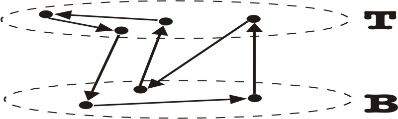
Figure 8: Fitting a cycle into two levels.

5 The $(j,k)$-Kemeny Rule

Suppose that $\{v_{1},\dots,v_{m}\}$ is a (finite) set of $m$ alternatives, and that voters in a finite set $N$ cast weak (or linear) order ballots, resulting in a profile $\Pi=\{\geq_{i}\}_{i\in N}$. The induced weighted tournament $\overrightarrow{\mathcal{H}_{\Pi}}=(\overrightarrow{V},\overrightarrow{E},\overrightarrow{w}_{\Pi})$ is as follows:

• $\overrightarrow{V}=\{v_{1},\dots,v_{m}\}$

• $\overrightarrow{E}=\{(v_{i},v_{j})\,|\,i<j\}$. Remark: This adds one edge for each two vertices.

• $\overrightarrow{w}_{\Pi}(v_{i},v_{j})=|\{t\in N\,|\,v_{i}\geq_{t}v_{j}\}|-|\{t\in N\,|\,v_{j}\geq_{t}v_{i}\}|$. These weights are voters’ net preferences for $v_{i}$ over $v_{j}$.

Definition 8

The $(j,k)$-Kemeny rule takes, as input, a profile $\Pi$ of $j$-chotomous weak orders on a finite set of alternatives, and outputs the $k$-chotomous weak order(s) on the alternatives corresponding to the solution(s) of max $k$-OP for $\overrightarrow{\mathcal{H}_{\Pi}}$. The $(j,\mathcal{L})$-, $(\mathcal{L},k)$- and $(\mathcal{L},\mathcal{L})$-Kemeny rules are defined similarly, with linear ordered ballots when $\mathcal{L}$ appears in the $j$ position, and linearly ordered outputs when $\mathcal{L}$ appears in the $k$ position. A $2_{r}$ in either position refers to r-valent dichotomous weak orders, corresponding to ordered $2$-partitions $\{T>B\}$ for which $|T|=r$.

Note that a dichotomous weak order $\{T>B\}$ can be interpreted as an approval ballot approving all alternatives in $T$. A $1$-valent (aka univalent) order $\{\{x\}>B\}$ can be interpreted as naming $x$ as winner (when it is the output) or as a plurality ballot for $x$ (when it is an input). The $r$-valent case with $r>1$ is also of interest for representing winning committees of exogenously specified size (as in ?; ?; ?). With that understanding, approval voting will be our first example of a special case of $(j,k)$-Kemeny. The list of such special cases contains a number of other familiar rules as well, including all in Table 2 (Section 1). Proofs justifying the Table 2 entries are straightforward, but (for reasons we discuss in the next section) these will appear in a later paper by ? (?). Our proof of Proposition 1 for approval voting should suffice to give the flavor:

Proposition 1

$(2,2_{1})$-Kemeny is approval voting, with outcome the approval winner(s).

Proof of Proposition 1: Consider a profile $\Pi^{\star}$ consisting of a single ballot $\{T>B\}$, corresponding to a single approval ballot of $T$, with induced weighted tournament $\overrightarrow{\mathcal{H}}_{\Pi^{\star}}=(\overrightarrow{V},\overrightarrow{E},\overrightarrow{w}_{\Pi^{\star}})$. It is easy to see that for any two alternatives $x$ and $y$, the weight $\overrightarrow{w}_{\Pi^{\star}}(x,y)$ on the $x\rightarrow y$ edge is the difference $\emph{App}_{\Pi^{\star}}(x)-\emph{App}_{\Pi^{\star}}(y)$ in their approval scores (which will be $+1$, $-1$, or $0$). Now consider a more general profile $\Pi$ with a number of ballots. The weight $\overrightarrow{w}_{\Pi}(x,y)$ on the $x\rightarrow y$ edge of $\overrightarrow{\mathcal{H}_{\Pi}}$ is likewise the difference $\emph{App}_{\Pi}(x)-\emph{App}_{\Pi}(y)$ in approval scores, because it is a sum of the contributions $\emph{App}_{\Pi^{\star}}(x)-\emph{App}_{\Pi^{\star}}(y)$ made by the individual ballots. The score of a univalent ordered partition $\{\{x\}>\overrightarrow{V}\setminus\{x\}\}$ will then be the sum

$$\Sigma_{y\in\overrightarrow{V}\setminus\{x\}}[\emph{App}(x)-\emph{App}(y)],$$

which is maximized when $x$ has a greatest approval score.  

The Theorem 2 results now lift immediately to $(j,k)$-Kemeny, showing:

Theorem 3

The problem of determining the winning ordering for a $(j,k)$-Kemeny election is in $P$ whenever $j$ or $k$ is equal to $2$ (or to $2_{r}$ for $r\geq 1$ any integer), and also whenever $\overrightarrow{w}_{\Pi_{\emph{cycle}}}=0$. In particular, winner determination is in $P$ for the first seven rules of Table 2. Also, for profiles satisfying $\overrightarrow{w}_{\Pi_{\emph{cycle}}}=0$, the $(j,\mathcal{L})$-Kemeny outcome is the linear ranking induced by Borda scores; in particular, the original Kemeny rule agrees with Borda.

We need to be a bit more careful when lifting the $\mathit{NP}$-hardness results from Theorem 1 to the context of $(j,k)$-Kemeny, however. To argue for $\mathit{NP}$-hardness when $j\geq 3$ or $j=\mathcal{L}$, we need to know that the specific weighted tournaments $\overrightarrow{\mathcal{H}_{\mathcal{G}}}$ constructed in the proofs of Theorems 1.2 and 1.3 are induced by some profile $\Pi$ of $j$-chotomous orders ($j\geq 3$), and for some profile of linear orders. Actually, from these proofs it can easily be seen that inducing some scalar multiple $C\overrightarrow{w}$ of the weights as $\overrightarrow{w}_{\Pi}$ would suffice, for each of these types of profile. But given an arbitrary integer-valued $\overrightarrow{w}$ for $V=\{v_{1},v_{2},v_{3},\dots,v_{m}\}$, and working for the moment with $j=3$, we can construct a profile of trichotomous weak orders satisfying $\overrightarrow{w}_{\Pi}=2\overrightarrow{w}$, as follows: the profile with two trichotomous weak orders

$$\Pi=\{v_{1}\}>\{v_{2}\}>\{v_{3},\dots,v_{m}\}\;;\;\{v_{3},\dots,v_{m}\}>\{v_{1}\}>\{v_{2}\}$$ (17)

satisfies $\overrightarrow{w}_{\Pi}(v_{1},v_{2})=2$ and assigns weight $0$ to every other edge. Thus by combining profiles similar to $\Pi$ we can build an arbitrary function $\overrightarrow{w}$ taking even integer values. For $j>3$, modify line 17 by breaking $\{v_{3},\dots,v_{m}\}$ into several pieces, ordered oppositely by the two orderings of $\Pi$. This constructions generalizes those by ? (?) and by ? (?). We have established:

Theorem 4

The problem of determining the winning ordering for a $(j,k)$-Kemeny election is $\mathit{NP}$-hard if $j\geq 3$ and $k\geq 3$ both hold or if $j=\mathcal{L}$ and $k\geq 3$ both hold. In particular winner determination is $\mathit{NP}$-hard for $(3,3)$-Kemeny.

None of our reasoning here shows $\mathit{NP}$-hardness when $k=\mathcal{L}$; in particular, Theorem 4 does not draw hardness conclusions for $(\mathcal{L},\mathcal{L})$-Kemeny (that is, for the original Kemeny rule itself) or for $(j,\mathcal{L})$-Kemeny with $j\geq 3$, because max cut is not polynomially reducible to “max $\mathcal{L}$-cut” (unless $\mathit{P=NP}$, of course). Nonetheless, our argument that computational complexity arises from the cyclic component also applies to the cases missing from Theorem 4. We already know (?) that the original Kemeny rule winner problem is $\mathit{NP}$-hard, and the last clause of Theorem 3 tells us that Kemeny reduces to a computationally easy rule when $\overrightarrow{w}_{\Pi_{\emph{cycle}}}=0$. As for $(j,\mathcal{L})$-Kemeny, we have just shown that for $j\geq 3$ the induced weights $\overrightarrow{w}_{\Pi}$ from profiles of $j$-chotomous weak orders are essentially as general as those arising from linear rankings, so winner determination is as hard as for the original Kemeny rule.

A second interesting question was raised by one of our COMSOC referees: what happens to tractability when the cyclic component is simple? What happens, for example, if $\overrightarrow{w}_{\emph{cycle}}$ can be written as a sum of only one or two simple cycles? We conjecture (but with low confidence) that winner determination for $(3,3)$-Kemeny would become tractable in this case. In this connection, it seems worth mentioning that the dimension of the cocyclic subspace grows linearly with the number of alternatives, while the dimension of the cyclic space grows quadratically. In a sense, then, the cyclic component is inherently the more complicated one, so that sharply limiting its complexity places a rather strong restriction on the underlying profile.

6 Connections:​ the Median Procedure, Generalized Scoring Rules,
     and Future Work

The $(j,k)$-Kemeny procedure presented here is closely related to, but distinct from, the median procedure (?; ?), a better-known general method for aggregating binary relations from one class into a relation from a possibly different class. When applied to the median procedure, several of the Table 2 restrictions yield the exact same aggregation rule as they do when applied to $(j,k)$-Kemeny; this happens, for example, when $j=\mathcal{L}$ or $k=\mathcal{L}$. In particular, the $(\mathcal{L},\mathcal{L})$-median procedure is the Kemeny voting rule, the $(2,\mathcal{L})$-median procedure yields, as outcome, the ranking by approval score, and the $(\mathcal{L},2_{1})$-median procedure yields the Borda winner(s).

But while $(2,2)$-Kemeny yields the mean rule, the $(2,2)$-median procedure does not (it seems unlikely that any reasonable version of the mean rule arises as a median procedure restriction) and the $(2,2_{1})$-median procedure provably differs from approval voting. So what explains the pattern of agreement and disagreement between these two general procedures?

We will address this issue in a planned sequel (?, ), but briefly sketch the analysis here. The median procedure (as well as the Kemeny voting rule) is commonly defined in terms of distance minimization via an appropriate metric $\delta$, but there is an equivalent inner product formulation that is a bit friendlier to the analysis we have in mind. Suppose we wish to aggregate a profile $\Pi=\{R_{i}\}_{i\in N}$ of binary relations belonging to some specified input class $\mathcal{I}$, to obtain a binary relation $S$ belonging to some specified output class $\mathcal{O}$. We represent each binary relation $R$ (on a set $A$ with $|A|=m$) via its symmetric characteristic vector $\mathbf{x}^{R}=(x^{R}_{1},x^{R}_{2},\dots,x^{R}_{m(m-1)})$; here $x^{R}_{i}=1$ if the $i^{\emph{th}}$ ordered pair (in some enumeration of all ordered pairs $(a,b)$ in $A\times A$ satisfying $a\neq b$) is a member of $R$, and $x^{R}_{i}=-1$ otherwise. Now each $R_{i}$ awards $\mathbf{x}^{R_{i}}\cdot\mathbf{x}^{S}$ points to any relation $S\in\mathcal{O}$. Sum these points over all $i\in N$ to obtain the score of $S$; the outcome of the aggregation is the $S\in\mathcal{O}$ with highest score.

This method coincides with the median procedure, as usually defined. Because the method awards points to binary relations rather than to the underlying alternatives in $A$, it constitutes a generalized scoring rule (in the sense of ?; ?; ?).

The difference between the median procedure and $(j,k)$-Kemeny can now be explained in terms of the vector space $\mathbb{R}^{m(m-1)}$ spanned by the characteristic vectors for all possible binary relations on $A$. This space is subject to a second orthogonal decomposition, of $\mathbb{R}^{m(m-1)}$ into symmetric and antisymmetric subspaces $\mathbf{V}\!_{sym}$ and $\mathbf{V}\!_{antisym}$ (see footnote 2). Here $\mathbf{V}\!_{sym}$ is the span of all characteristic vectors $\mathbf{x}^{R}$ of symmetric binary relations (satisfying $(a,b)\in R\Leftrightarrow(b,a)\in R$) and $\mathbf{V}\!_{antisym}$ is the span of vectors $\mathbf{x}^{R}$ of antisymmetric binary relations (satisfying $(a,b)\in R\Leftrightarrow(b,a)\notin R$). Let $asym(\mathbf{x}^{R}$) denote the orthogonal projection of $\mathbf{x}^{R}$ onto $\mathbf{V}\!_{antisym}$.

We obtain an equivalent formulation of $(j,k)$-Kemeny by modifying the inner product version of the median procedure (as defined two paragraphs previous) as follows: use $asym(\mathbf{x}^{R_{i}})\cdot asym(\mathbf{x}^{S})$ in place of the original $\mathbf{x}^{R_{i}}\!\cdot\mathbf{x}^{S}$. The matter of whether some particular restriction of the median procedure agrees with the corresponding restriction for $(j,k)$-Kemeny now comes down to the role of the symmetric component in the aggregation. If either $\mathcal{I}$ or $\mathcal{O}$ live entirely within $\mathbf{V}\!_{antisym}$, the symmetric component has no effect on the aggregation – projection onto $\mathbf{V}\!_{antisym}$ thus has no effect on the points awarded, and the restriction of the median procedure via $\mathcal{I}$ and $\mathcal{O}$ coincides with the corresponding restriction for $(j,k)$-Kemeny. In particular, this is what happens whenever linear rankings are used as $\mathcal{I}$ or as $\mathcal{O}$; it does not happen when $\mathcal{I}$ = $\mathcal{O}$ = the class of dichotomous weak orders.

Thus, while the proofs justifying lines of Table 2 are straightforward, we prefer to postpone these arguments to a planned sequel (?, ), which will focus on the role of orthogonal decomposition in these sorts of procedures and in the families of specific rules that arise as their restrictions. There we will explore more precisely the exact relationships between special cases of the median procedure, and corresponding special cases of $(j,k)$-Kemeny.

Acknowledgments

We thank Matthew Anderson, Markus Brill, Dominik Peters, and Alan D. Taylor for help with content and presentation, and the referees for an earlier (COMSOC 2016 conference) version, for suggesting interesting follow-up questions. Comments by the journal referees significantly improved clarity and organization.

References

- Aziz et al. Aziz, H., Brill, M., Conitzer, V., Elkind, E., Freeman, R., and Walsh, T. (2017). Justified representation in approval-based committee voting. Social Choice and Welfare, 48, 461–485.
- Barthélemy and Monjardet Barthélemy, J. P., and Monjardet, B. (2009). The median procedure in cluster analysis and social choice theory. Mathematical Social Sciences, 1, 235–267.
- Bartholdi et al. Bartholdi, J. I., Tovey, C. A., and Trick, M. A. (1989). Voting schemes for which it can be difficult to tell who won the election. Social Choice and Welfare, 6, 157–165.
- Brandl et al. Brandl, F., Brandt, F., and Seedig, H. G. (2016). Consistent probabilistic social choice. Econometrica, 84(5), 1839–1880.
- Brandl and Peters Brandl, F., and Peters, D. (2017). An axiomatic characterization of the Borda mean rule. In Proceedings of the 11th Multidisciplinary Workshop on Advances in Preference Handling (MPREF), to appear.
- Conitzer et al. Conitzer, V., Rognlie, M., and Xia, L. (2009). Preference functions that score rankings and maximum likelihood estimation. In Proceedings of the Twenty-First International Joint Conference on Artificial Intelligence (IJCAI-09), pp. 109–115.
- Croom Croom, F. (1978). Basic Concepts of Algebraic Topology. New York: Springer-Verlag.
- Debord Debord, B. (1987). Caractérisation des matrices des préférences nettes et méthodes d’aggrégation associées. Mathématiques et sciences humaines, 97, 5–17.
- Duddy and Piggins Duddy, C., and Piggins, A. (2013). Collective approval. Mathematical Social Sciences, 65, 190–194.
- Duddy et al. Duddy, C., Piggins, A., and Zwicker, W. S. (2016). Aggregation of binary evaluations: a Borda-like approach. Social Choice and Welfare, 46, 301–322.
- Elkind et al. Elkind, E., Faliszewski, P., Skowron, P., and Slinko, A. (2017). Properties of multiwinner voting rules. Social Choice and Welfare, 48, 599–632.
- Fishburn Fishburn, P. (1977). Condorcet social choice functions. SIAM Journal on Applied Mathematics, 33, 469–489.
- Hammer et al. Hammer, P. L., Ibaraki, T., and Peled, U. N. (1981). Threshold numbers and threshold completions. Annals of Discrete Math, 11, 125–145.
- Harary Harary, F. (1959). Graph theory and electrical networks. IRE Trans. Circuit Theory, 6(5), 95–109.
- Hemaspaandra et al. Hemaspaandra, E., Spakowski, H., and Vogel, J. (2005). The complexity of Kemeny elections. Theoretical Computer Science, 349, 382–391.
- Hudry Hudry, O. (2012). On the computation of median linear orders, of median complete preorders and of median weak orders. Mathematical Social Sciences (special issue on Computational Foundations of Social Choice), 64, 2–10.
- Kilgour Kilgour, D. M. (2010). Approval balloting for multi-winner elections. In Laslier, J.-F., and Sanver, M. R. (Eds.), Handbook on Approval Voting, pp. 105–124. Springer-Verlag.
- Kirchoff Kirchoff, G. (1847). Über die Auflösung der Gleichungen, auf welche man bei der Untersuchung der linearen vertheilung galvanischer Ströme geführt wird. Annalen der Physik, 148(12).
- MacWilliams MacWilliams, F. J. (1958). An algebraic proof of Kirchoff’s network theorem. Bell Telephone Laboratories Memorandum.
- McGarvey McGarvey, D. C. (1953). A theorem on the construction of voting paradoxes. Econometrica, 21(4), 608–610.
- Myerson Myerson, R. B. (1995). Axiomatic derivation of scoring rules without the ordering assumption. Social Choice and Welfare, 12, 59–74.
- Saari Saari, D. (1994). Geometry of Voting. Springer.
- Xia and Conitzer Xia, L., and Conitzer, V. (2011). A maximum likelihood approach towards aggregating partial orders. In Proceedings of the 22nd International Joint Conference on Artificial Intelligence (IJCAI-11), pp. 446–451.
- Young Young, H. P. (1974). An axiomatization of Borda’s rule. Journal of Economic Theory, 9, 43–52.
- Zwicker Zwicker, W. S. (1991). The voters’ paradox, spin, and the Borda count. Mathematical Social Sciences, 22, 187–227.
- Zwicker Zwicker, W. S. (2008). Consistency without neutrality in voting rules: When is a vote an average?. Mathematical and Computer Modelling (special issue on Mathematical Modeling of Voting Systems and Elections: Theory and Application).
- Zwicker Zwicker, W. S. (2018). Orthogonal decomposition and the aggregation of binary relations. Working Paper.