Superiorized iteration based on proximal point method and its application to XCT image reconstruction

Abstract In this paper, we investigate how to determine a better perturbation for superiorized iteration. We propose to seek the perturbation by proximal point method. In our method, the direction and amount of perturbation are computed simultaneously. The convergence conditions are also discussed for bounded perterbation resilence iteration. Numerical experiments on simulated XCT projection data show that the proposed method improves the convergence rate and the image quality.

Keywords Superiorization of iteration; Proximal point method; XCT image reconstruction; Bounded perturbation resilience

1 Introduction

Linear imaging problems, such as X-ray computed tomography(XCT), single-photon emission computed tomography(SPECT) and magnetic resonance imaging (MRI) can be formulated by

$$Ax=b,$$ (1)

where the imaging matrix $A\in\mathbb{K}^{m\times n}$, the observed data $b\in\mathbb{K}^{m}$, and $x\in\mathbb{K}^{n}$ is the image to be reconstructed[1, 2]. $\mathbb{K}$ can be the real number field $\mathbb{R}$ or the complex number field $\mathbb{C}$.

Iterative methods, such as algebraic reconstruction technique(ART)[3, 4, 5] and expectation maximum(EM)[6], are usually used to solve (1) because of the ill-posedness of $A$ and huge data dimension for practical problems[1, 7]. However, the reconstructed results by iteration methods mentioned above are not satisfied when the $m\ll n$, such as few-angle and sparse-angle XCT. Regularization methods based on optimization are investigated to improve the image quality (see [8, 9, 10] and references therein). However, we are short of efficient algorithm to solve the optimization problem because the dimension is huge for imaging problems[11, 12]. Superiorization of iteration was proposed to seek a desirable result from the application point of view at a relatively low computational cost.

In order to introduce the concept of superiorization, we consider the following constrained optimization problem for (1)

$$\min\phi(x)\quad\text{subject to }\quad Ax=b\text{ and }x\in C_{0},$$ (2)

where the convex function $\phi$ and the convex set $C_{0}$ denote the prior knowledge of the solution $x$. In this paper, we assume that $C_{0}$ is a bounded set in $\mathbb{K}^{n}$ because the desired images are bounded in practice. Let $C_{i}=\{x\in\mathbb{R}^{n}|\langle a^{i},x\rangle=b_{i}\}(i=1,2\cdots,m)$ with $a^{i}$ denoting the $i$-th row of $A$, and the optimization problem (2) can be written as

$$\min\phi(x)\quad\quad\mathrm{subject~{}to}\quad\quad x\in C\triangleq\bigcap_{i=0}^{m}C_{i}.$$ (3)

As mentioned above, we can use ART or EM iteration to find a feasible point in $C$[3, 4, 5, 7], but we are short of efficient algorithm to solve (3), i.e. look for a point $x^{\ast}\in C$ such that $\phi(x^{\ast})\leq\phi(x)\forall x\in C$, since the dimension is huge for imaging problems [11, 12]. The aim of superiorized iteration is to steer the iterates toward a superior point $x^{\star}\in C$ such that $\phi(x^{\star})$ is smaller but not necessarily smallest. There are three reasons to propose and use the superiorization approach.

1. The computational cost to solve the large scale constrained optimization problems is very high, especially when the constraint set $C$ is a complicated convex set(for example $C$ is the intersection of a series of convex sets).

2. We need not to solve the constraint optimization problem (3) precisely since the optimal solution of (2) is possibly not the solution we want in practical problems[12, 4]. For example, the optimal solution often suffers from staircase problem if $\phi$ is the total variation function[13, 14, 15].

3. The convergence rate could be improved by using appropriate perturbed directions and amounts in our opinion.

Superiorization of iterative methods have been used in various image reconstruction problems, such as XCT [11, 16, 10, 17], SPECT [18], bioluminescence tomography [19] and proton computed tomography[20, 21], since it was proposed. Under the assumption that $x^{k+1}=Px^{k}$ converge to a feasible point $x^{\ast}\in C$, the superiorized version of $P$ with respect the objective function $\phi$ (2) can be written as[12]

$$\left\{\begin{array}[]{lcl}y^{k}&=&x^{k}+\beta_{k}v^{k}\\ x^{k+1}&=&Py^{k}\end{array}\right.,$$ (4)

where $v^{k}$ is a descent direction of $\phi$ at $x^{k}$, and $\beta_{k}>0$ such that $\phi(y^{k})\leq\phi(x^{k})$ and $\mathrm{dist}(x^{k+1},C)<\mathrm{dist}(x^{k},C)$[12, 17]. There are two key problems of superiorized iteration (4) to be answered

1. Under what conditions the iteration sequence of (4) is convergent.

2. Is the limit $x^{\star}$in the constraint set $C$ if the sequence is convergent?

3. How to determine better perturbation direction $v^{k}$ and amount $\beta_{k}$ to guarantee the convergence of iteration (4)?

4. Can we attain our aim that $\phi(x^{\star})\leq\phi(x^{\ast})$ where $x^{\star},x^{\ast}$ are the limits of the superiorized iteration sequence and the original iteration sequence without perturbation, respectively.

As far as we know, the studies on superiorized algorithms are about the first two problems[22, 17, 23, 24]. A condition called bounded perturbation resilience(BPR, see section 2 for the definition) of iteration plays an important role in the proof of perturbed version of iteration algorithm. For a BPR iteration $P$, the sequence generated by (4) converges to a feasible point if the perturbation is summable, i.e. $\sum_{k=1}^{\infty}\|\beta_{k}v^{k}\|=\sum_{k=1}^{\infty}|\beta_{k}|<\infty$. Therefore, it is only required that the perturbation is summable for the BPR iteration $P$ to guarantee the convergence of iteration (4). The ART iteration and its variations, such block iteration projection(BIP)[11] and string averaging projection (SAP)[16], were proved to be bounded perturbation resilient when the constraints are consistent. For inconsistent cases, the authors of [17] proved the convergence of the symmetric version of ART under summable perturbations. The convergence and perturbation resilience of dynamic string-averaging projection algorithms were studied in [23] recently. The superiorization of EM algorithm was proposed in [19], and then a modified version and some assumptions for convergence were studied in [18]. Furthermore, the bounded perturbation resilience(BPR) of EM algorithms was proved in [24].

We attempt to study the third problem in this paper. It is obvious that the variables $\{v^{k}\}$ and $\{\beta_{k}\}$ play an important role in he convergence rate and quality of reconstructed images. In the literature, parameters $v^{k}$ and $\beta_{k}$ are determined by two successive steps for each iteration. Firstly, an unit descent direction of $\phi$ at $x^{k}$ is usually as $v^{k}$ [12, 17, 11, 16]. Secondly, the parameters $\beta_{k}$ is adjusted by the criterion that $\phi(x^{k}+\beta_{k}v^{k})\leq\phi(x^{k})$ and $\text{dist}(P(x^{k}+\beta_{k}v^{k}),C)<\text{dist}(x^{k},C)$. Numerical experiments showed that one should adjust $\beta_{k}$ by trial and error such that $\phi(x^{k}+\beta_{k}v^{k})\leq\phi(x^{k})$ and $\text{dist}(P(x^{k}+\beta_{k}v^{k}),C)<\text{dist}(x^{k},C)$. And these operations make the computational cost much more high.

In this paper, we propose a new method to determine the perturbed results $y^{k}$ directly, rather than the middle variables $v^{k}$ and $\beta_{k}$. And the direction and amount of perturbation can be obtained by $\beta_{k}v^{k}=y^{k}-x^{k}$ simultaneously. The proposed method determines the perturbed result $y^{k}$ by optimization method with single regularization parameter. In fact, $y^{k}$ is a proximate point of $x^{k}$ with respect to $\phi$. We can prove that the inequality $\phi(y^{k})\leq\phi(x^{k})$ holds naturally. Therefore, we only need to adjust the regularization parameter in the optimization problem such that $\text{dist}(P(y^{k}),C)<\text{dist}(x^{k},C)$. Therefore, the computation cost could be reduced intuitively. Moreover, numerical experiments on XCT image reconstruction show that the convergence rate and quality of reconstruction images can be improved by the proposed method. Furthermore, the convergence of the proposed algorithm is investigated theoretically. We call the proposed algorithm as $\phi$-proximate point superiorization ($\phi$-PP superiorization) algorithm in the following to emphasize the perturbed point $y^{k}$ is the $\phi$-proximate point of $x^{k}$. As for the fourth problem, there is no progress as far as we known.

The rest of this paper is organized as follows. In section 2, we present the proposed superiorization algorithm and theory analysis. Several numerical experiments are present to demonstrate the efficiency of the proposed superiorization algorithm in section 3. Section 4 contains the conclusions and future works.

2 $\phi$-proximate point($\phi$-PP) superiorization algorithm and theory analysis

2.1 $\phi$-PP superiorization algorithm

Let $P$ be an iteration for the feasible problem $x\in\bigcap_{i=0}^{m}C_{i}$. The superiorized version of $P$ can be illustrated algorithm 1.

Algorithm 1 $\phi$-proximate point superiorzation algorithm

1:  set $k=0$, $x^{0}\in{\mathbb{R}^{n}}$, $\beta_{0}>0$, and $0<\gamma<1$.

2:  while $k\leq{M}$ and $\textrm{Res}(x^{k})\geq{\epsilon}$

3:    logic=true;

4:    while(logic)

5:        $y^{k}=\mathrm{perturb}_{\phi}(x^{k},\beta_{k})$

6:        $x^{k+1}=Py^{k}$

7:        if $\phi(y^{k})\leq\phi(x^{k})$ and $(\textrm{dist}(x^{k+1},C)<\textrm{dist}(x^{k},C))$($\ast$)

8:           logic=false

9:        else

10:          $\beta_{k}={\beta_{k}}{\gamma}$

11:        end(if)

12:     end(while)

13:     $\beta_{k+1}={\beta_{k}}{\gamma}$

14:     $k=k+1$

15:  end(while)

There are two methods to compute $\textrm{dist}(x,C)$[17, 11],

$$\textrm{dist}(x,C)=\sqrt{\sum_{j=1}^{m}\left(\frac{b_{j}-\langle a^{j},x\rangle}{\|a_{j}\|}\right)^{2}},$$ (5)

and

$$\textrm{dist}(x,C)=\sqrt{\sum_{j=1}^{m}\left(b_{j}-\langle a^{j},x\rangle\right)^{2}}\triangleq\text{Res}(x).$$ (6)

The first method is unstable because small changes in the data $x$ result in large changes in the value of dist$(x,C)$ [17]. Therefore, we use the second formula to measure the deviation between the projection of reconstructed image $x$ and the observed data.

In the classical superiorization algorithm( see [11, 16, 17] and references therein), $y^{k}=\textrm{perturb}_{\phi}(x^{k},\beta_{k})=x^{k}+\beta_{k}v^{k}$, where $v^{k}=\left\{\begin{array}[]{cl}-{u^{k}\over\|u^{k}\|},&u^{k}\neq 0\\ 0&u^{k}=0\end{array}\right.$ with $u^{k}\in\partial\phi(x^{k})$ being fixed as a subgradient of $\phi$ at $x^{k}$. Then $\beta_{k}$ is adjusted to make the condition ($\ast$) true. Because the perturbation direction $v^{k}$ is fixed, it is possible to adjust $\beta_{k}$ many times, and the computational cost is increased.

In this paper, we propose to compute the perturbed vector $y^{k}$ directly by solving the following optimization problem

$$y^{k} =\text{perturb}_{\phi}(x^{k},\beta_{k})=\text{arg}\min_{y}\phi(y)+{1\over 2\beta_{k}}\|y-x^{k}\|_{2}^{2}.$$ (7)

Let $\psi(y)=\phi(y)+{1\over 2\beta_{k}}\|y-x^{k}\|_{2}^{2}$, and we have

$$\phi(y^{k})\leq\psi(y^{k})\leq\psi(x^{k})=\phi(x^{k}),$$ (8)

Therefore, the first condition in ($\ast$) is naturally true for the proposed method. Moreover, it is obvious that the perturbation $y^{k}-x^{k}$ by our method is dependent on the parameter $\beta_{k}$, and the perturbation direction and amount change simultaneously along with the change of $\beta_{k}$, while the classic method change the perturbation amount only.

It seems that the optimization problem (7) could increase the computational cost of superiorization algorithm. However, the experiments show that the convergence rate is accelerated by using the proposed perturbation, and the computational cost can be reduced by the same terminated criterion since the number of iteration is smaller. Furthermore, for the commonly used regularization function $\phi$, we have explicit solution or efficient algorithm for the regularization problem (7), such as

Example 1.

$\phi(x)=\|x\|_{0}$, $y^{k}_{i}=\mathrm{hard}_{\phi}(x^{k}_{i},{\beta_{k}})=\left\{\begin{array}[]{cl}x_{i}&|x_{i}|>\beta\\ 0&\textrm{otherwise}\end{array}\right.$;

Example 2.

$\phi(x)=\|x\|_{1}$, $y^{k}_{i}=\mathrm{soft}_{\phi}(x^{k}_{i},{\beta_{k}})=\max\{|x_{i}|-\beta_{k},0\}\textrm{sign}(x_{i})$;

Example 3.

$\phi(x)={1\over 2}\|x\|_{2}^{2}$, $y^{k}_{i}={x_{i}^{k}\over\beta_{k}+1}.$

Example 4.

For the total variation regularization, $\phi(x)=\sum_{i=1}^{n}|\nabla x_{i}|$[13], we can apply fast algorithms, such as dual algorithm [25], splitting Bregman iteration [26], fixed point method[27] and ADMM method[28], to solve (7). In this paper, we the dual algorithm 2 (see [25] for details) to solve the subproblem (7).

Algorithm 2 Dual algorithm for TV-minization [25].

   Let $p^{0,k}=0$, $0<\tau<1/8$ and $N>0$,

   for s=0:(N-1),

$$p_{i,j}^{s+1,k}=\frac{p_{i,j}^{s,k}+\tau(\nabla(\textrm{div}p^{s,k}-x^{s,k}/\beta_{k}))_{i,j}}{1+\tau|(\nabla(\textrm{div}p^{s,k}-x^{s,k}/\beta_{k}))_{i,j}|},$$ (9)

   end(for)

  $y^{k}=x^{k}-\beta_{k}\textrm{div}(p^{N,k})$;

2.2 Convergence of the $\phi$-PP superiorization algorithm

We will investigate the convergence of the $\phi$-PP superiorization algorithm in this subsection. Before illustrating the convergence of algorithm 1, we first review the BPR condition.

Definition 1.

Bounded perturbation resilience [12]: An iterative operator $P:\mathbb{R}^{n}\longrightarrow{\mathbb{R}^{n}}$ is said to be bounded perturbation resilience with respect to a given nonempty set $C\subseteq\mathbb{R}^{n}$ if the following is true: If a sequence $\{x^{k}\}_{k=0}^{\infty}$, obtained by the iterative process

$$x^{k+1}=Px^{k},~{}~{}~{}~{}~{}\textrm{for all}~{}~{}~{}k\geq 0,$$ (10)

converges to a point in $C$ for all $x^{0}\in{\mathbb{R}^{n}}$, then the iterative sequence $\{x^{k}\}_{k=0}^{\infty}$

$$x^{k+1}=P(x^{k}+v^{k}),~{}\textrm{for all}~{}k\geq{0},$$ (11)

also converges to a point in $C$ for all $x^{0}\in{\mathbb{R}^{n}}$ provided that $\displaystyle\mathop{\sum}_{k=1}^{\infty}\|v^{k}\|_{2}<\infty$.

Let $P_{i}$ be the projection operator on $C_{i}(i=0,1,\cdots,m)$, i.e. $P_{i}x=\min_{y\in C_{i}}\|x-y\|_{2}$. For $i=1,2\cdots,m$, we have

$$P_{i}x = x+\frac{b_{i}-\langle{a^{i},x}\rangle}{||a^{i}||^{2}_{2}}(a^{i})^{t},\qquad i=1,2,\cdots,m.$$ (12)

In practice we can select simple convex set $C_{0}$, $C_{0}=\{x\in\mathbb{R}^{n}|0\leq x_{i}\leq L,i=1,2,\cdots,n\}$ for instance, such that $P_{0}x$ have explicit solution. The classic ART iteration and its variations (block iteration projection[4] and successive averaging projection[5] for example) by the $P_{i}(i=0,1,\cdots,m)$ are all nonexpansive and BPR operator [11, 16]. Becuase the desirable solutions of (2) are bounded in practice, we define $P=P_{0}\hat{P}$ with $\hat{P}$ denoting the ART iteration and its variations. Therefore, the iteration sequence $\{x^{k}\}\subset C_{0}$ is bounded, i.e. there is a number $R$ such that $\|x^{k}\|\leq R$ for all $k\in\mathbb{N}$.

Under the assumption that $P$ is BPR iteration(ART iterations and EM iterations for example), we only need to prove $\sum_{k}\|y^{k}-x^{k}\|_{2}<\infty$ to show the convergence of algorithm 1, and we have the following theorem about algorithm 1.

Theorem 1.

Assume that $\phi(x)$ is a nonnegative and closed convex function on $\mathbb{R}^{n}$, $P$ is a continuous and BPR iteration for feasible problem $x\in\bigcap_{i=0}^{n}C_{i}$, and $Px\in C_{0}$ is bounded for all $x\in\mathbb{R}^{n}$. Then, we have

1. The sequence $\{y^{k}\}$ in algorithm 1 is bounded,

2. For a given bounded set $B_{0}\subset\mathbb{R}^{n}$, there is a real number $M>0$ such that $|\partial\phi(x)|<M$ for all $x\in B_{0}$,

3. $\sum_{k=0}^{+\infty}\|y^{k}-x^{k}\|<+\infty$.

In other word, the iteration sequence $\{x_{k}\}$ generated by algorithm 1 converges to a feasible point in $C$ if $P$ is a BPR operator.

Proof.

Statement 1
Firstly, we have the sequence $\{x^{k}\}\subset C_{0}$ is bounded based on the assumption of $P$, and there is a positive number $R$ such that $\|x^{k}\|\leq R$ for all $k\geq 0$. Secondly, $\phi$ is a continuous function on $C_{0}$ [29], and then there are a real number $M_{1}$ such that $\phi(x)\leq M_{1}$ for all $x\in C_{0}$.

Since $y^{k}$ is the solution of (7), by selecting $y=x^{k}$ in (7) we have

$$\phi(y^{k})+\frac{1}{2\beta_{k}}\|y^{k}-x^{k}\|^{2}_{2}\leq\phi(x^{k}).$$ (13)

Therefore, we have

$$\frac{1}{2\beta_{k}}\left(\|y^{k}\|^{2}_{2}-\|x^{k}\|^{2}_{2}\right)\leq\phi(y^{k})+\frac{1}{2\beta_{k}}\|y^{k}-x^{k}\|^{2}_{2}\leq\phi(x^{k})\leq M_{1}.$$ (14)

The equality (14) can be written as

$$\|y^{k}\|\leq\|x^{k}\|+2\beta_{k}\phi(x^{k})\leq R+2\beta_{k}M_{1}.$$ (15)

Because $\{\beta_{k}\}$ is a positive and summable sequence, there exists a positive number $M_{2}=R+2M_{1}\sum_{k=1}^{\infty}\beta_{k}$ such that

$$\|y^{k}\|\leq M_{2}.$$ (16)

Statement 2
For the given bounded set $B_{0}$, let $B_{1}=\{x+y|x\in C_{0},y\in\mathbb{R}^{n}~{}\text{and}~{}\|y\|_{2}\leq 1\}$. Therefore, $B_{0}\subset B_{1}$, and there is a real number $M_{3}>0$ such that $|\phi(y)|\leq M_{3}$ for all $y\in B_{1}$ by the assumption of $\phi$[29]. In order to prove the conclusion, we need to prove there exist a real number $M_{4}$ such that $\max_{\hat{x}\in\partial\phi(x)}\|\hat{x}\|\leq M_{4}$ for $\forall x\in B_{0}$.

Let $x\in B_{0}$ and $\hat{x}\in\partial\phi(x)$. Then for all $z\in\mathbb{R}^{n}$ we have

$$\phi(z)-\phi(x)\geq\langle\hat{x},z-x\rangle.$$ (17)

Furthermore, we can choose an appropriate $y\in B_{1}$ such that $\langle\hat{x},z-x\rangle\geq\|\hat{x}\|$. In fact, if $\hat{x}=0$, it is obvious that $\langle\hat{x},z-x\rangle\geq\|\hat{x}\|$. Otherwise, one can choose $z=x+{\hat{x}\over\|\hat{x}\|}\in B_{1}$ such that $\langle\hat{x},z-x\rangle\geq\|\hat{x}\|$. Therefore, we have

$$\|\hat{x}\|\leq{|\phi(z)|+|\phi(x)|}\leq 2M_{3},$$ (18)

i.e. $\max_{\hat{x}\in\partial\phi(x)}\|\hat{x}\|\leq 2M_{3}$ for $\forall~{}x\in B_{0}$. The second statement is true by selection $M_{4}=2M_{3}$.
Statement 3

Let $y^{k}$ is the solution of (7), and then we have

$$0\in\partial\phi(y^{k})+{1\over\beta_{k}}(y^{k}-x^{k}).$$ (19)

Therefore, the $\phi$-PP perturbation $v^{k}=y^{k}-x^{k}\in\beta_{k}\partial\phi(y^{k})$. Assuming $B_{0}=\{x\in\mathbb{R}^{n}|~{}\|x\|_{2}\leq M_{2}\}$ in the second statement, we have $y^{k}\in B_{0}$ and

$$\sum_{k}\|v^{k}\|=\sum_{k}\beta_{k}\|\partial\phi(y^{k})\|\leq M_{4}\sum_{k}\beta_{k}<\infty.$$ (20)

Moreover, the iteration sequence converges to a feasible point in $C=\bigcap_{i=0}^{n}C_{i}$ if the iteration operator $P$ is BPR. ∎

Remark 1.

Based on the assumption of iteration $P$, the $\phi$-PP superiorized version of ART-like converge to a feasible point. In addition the conclusion can be generalized for EM iteration by imposing some conditions.

3 Numerical experiments for XCT image reconstruction

Although superiorization algorithms can be applied to different image reconstruction methods[4, 18, 19], we present the application of the proposed superiorization algorithm to XCT image reconstruction to verify the efficiency of the $\phi$-PP superiorization algorithm.

In our simulations, we used the total variation(TV) function as the objective function $\phi$ [13, 17, 16, 8]. For a $K\times{L}$ digital image $x$, the discrete total variation of $x$ is defined as

$$TV(x)=\sum_{i=1}^{K-1}\sum_{j=1}^{L-1}\sqrt{(x_{i+1,j}-x_{i,j})^{2}+(x_{i,j+1}-x_{i,j})^{2}}.$$ (21)

Furthermore, we used the classic ART iteration $P=P_{0}P_{m}\cdots P_{1}$ as the iteration operator $P$ in our numerical experiments. In order to compare the proposed superiorization algorithm with the classic superiorization algorithm, we applied the classic superiorization and $\phi$-PP superiorization algorithm to two phantoms (see figure 1). The first one is the $200\times 200$ Shepp-Logan phantom[30], and the second one is the $256\times 256$ head phantom with a ghost which is invisible at 22 specified projection directions [10, 31]. In addition, we compare the performances of the two algorithms for the noiseless and noised data with different projections. In all experiments, the noised projection data was corrupted by additive Gaussian white noise with variance $\sigma^{2}=0.0001$. We record the iterations, running time of program and mean square error (MSE) of different algorithms, where MSE is computed by

$$MSE(x)=\sqrt{{1\over KL}\sum\limits_{i=1,j=1}^{K,L}\left(x_{ij}-x^{0}_{ij}\right)^{2}},$$ (22)

where $x^{0},x$ are the original and estimated images, respectively.

We abbreviate the classic TV-superiorization algorithm as TV-S, and the proposed algorithm as TV-PPS for convenience. In the numerical experiments, we used the initial value $x^{0}=\mathbf{0}$, $\beta_{0}=10$, $\gamma=1/2$, and $\textrm{dist}(x^{k},C)=\text{Res}(x)=\|Ax^{k}-b\|_{2}$ in algorithm 1.

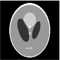
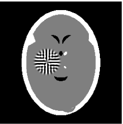
Figure 1: Shepp-Logan phantom (a) and ghost phantom(b).

3.1 Shepp-Logan phantom

Noiseless projection data: The projection data were collected by calculating line integrals across the phantom at 60, 90, 120 directions(equal increments $3^{\circ},2^{\circ}$ and $1.5^{\circ}$ from $0^{\circ}$ to $180^{\circ}$) of 201 equally spaced parallel lines from $-1$ to $1$. Iteration procedures were terminated when $\textrm{Res}(x^{k})\leq{0.01}$ for the noiseless experiments.

The reconstruction images from the noiseless projection data were shown in the Fig. 2. From Fig. 2, we can observe that the classic and the proposed algorithms can reconstruct images from the three projection data. In order to show the advantages of the proposed algorithm visually, the central vertical line of the differences between the reconstructed images and the original image are present in Fig. 3. We can observe that the $\phi$-PP superiorization is more efficient than the classic superiorization in the aspect of suppressing the artifacts in the reconstructed images.

(a) TV-S

(b) TV-S

(c) TV-S

(d) TV-PPS

(e) TV-PPS

(f) TV-PPS

Figure 2: The reconstruction results of Shepp-Logan phantom from 3 noiseless data sets. The images in first row are reconstructed by TV-S algorithm, and the images in second row by TV-PPS algorithm. From left to right, the images in each column are the reconstruction results from 60, 90, and 120 projections.

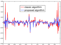
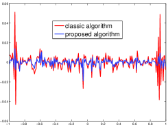
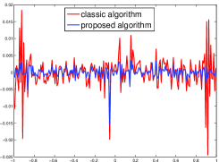
(a)	(b)	(c)

Figure 3: Comparison of profiles. (a), (b), (c) are the profile differences of the central vertical lines of the images in Fig. 2 and the original image.

In order to compare the images in Fig. 2 quantitatively, we tabulated the iterations, MSE, Res and running time(RT) of programs in Table 1. By comparing the numbers in Table 1, we can draw the conclusion that the proposed method can improve the quality of the estimated images and save computation time.

Table 1: The MSE, number of iteration and running time(RT) of the images in Fig.  2

Algorithm	TV-S	TV-PPS	TV-S	TV-PPS	TV-S	TV-PPS
projections	120	120	90	90	60	60
iterations	103	97	75	67	67	44
MSEs	0.0059	0.0022	0.0102	0.0046	0.0181	0.0097
RT(min)	15.179	11.3611	5.5021	5.3384	4.4305	3.0206

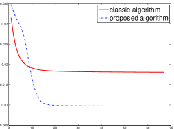
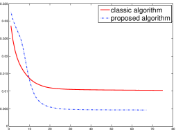
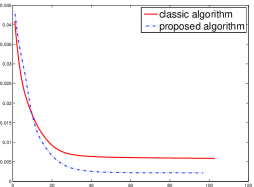
Figure 4: MSE vs. iteration number of the two algorithms for Shepp-Logan phantom, from left to right for 60, 90, and 120 projections.

In order to compare the convergent speed of the proposed algorithms with the classic algorithms visually, we present the evolution of MSE along with the iteration process in Fig. 4 for the 3 projection data. And we can observe that the proposed perturbation can accelerate the convergent rate and improve the reconstructed image qualities.

Noised projection data: In order to show the ability of noise suppressing, we apply the algorithms to noised projection data. For the noise experiments, the iteration procedures were terminated the algorithms when $\textrm{Res}(x^{k})\leq{0.1},0.12,0.14$ for 60, 90 and 120 projections. The reconstruction images were given in Fig. 5, and Table 2 showed the MSE, number of iterations, running time of different images in Fig. 5.

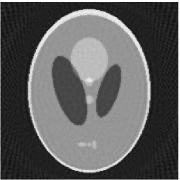
(a) TVS

(b) TVS

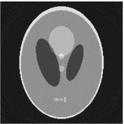
(c) TVS

(d) TV-PPS

(e) TV-PPS

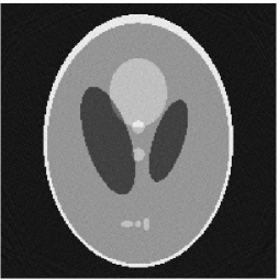
(f) TV-PPS

Figure 5: The reconstruction results of Shepp-Logan phantom from noised projections. From left to right, the images in each column are reconstructed from 60, 90, and 120 projections.

Table 2: The MSE, number of iteration and running time(RT) of images in Fig.  5

Algorithm	TV-S	TV-PPS	TV-S	TV-PPS	TV-S	TV-PPS
projections	120	120	90	90	60	60
iterations	49	49	34	33	25	24
MSEs	0.0134	0.0108	0.0132	0.0085	0.0192	0.0112
RT(min)	5.6175	6.6477	2.8230	2.5867	1.5444	1.4879

By comparing Fig. 5 and Table 2, we can observe the reconstructed images by the proposed superiorization algorithm have higher quality than these by classic superiorization algorithm. Therefore, the performance of the proposed superiorization algorithm is better than the classic superiorized algorithms for noised projection data.

In summary, the proposed superiorization algorithm has faster reconstruction speed than the classic superiorization algorithms, and the MSEs of the reconstruction images by the proposed algorithm are smaller than these of the reconstructed images by the classic superiorization algorithm regardless noiseless and noised projection data. Therefore, the above results demonstrate that the modified superiorization algorithm can accelerate the convergent speed and improve the image qualities.

3.2 Ghost phantom

Noiseless projection data: Since the ghost in this phantom is invisible at 22 directions [10, 11], the reconstruction images usually suffer from artifacts. in our simulations, the projection data were collected in 112 and 82 directions: 90 and 60 with equal angle increments from $0^{\circ}$ to $179^{\circ}$ and 22 specified views in which the ghost is invisible [10]. Iteration procedures were terminated when $\textrm{Res}(x^{k})\leq{0.01}$ for the noiseless projections.

The reconstruction images from the noiseless projection data were shown in the Fig. 6. For comparison, Table 3 present the iterations, MSE, Res and running time(RT) of different reconstruction results.

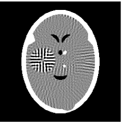
TV-S	TV-S
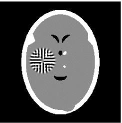
TV-PPS	TV-PPS

Figure 6: The reconstruction results of ghost phantom from noiseless projections. From left to right, images in each column are reconstructed from 82, 112 projections .

Table 3: The MSE, number of iteration and running time(RT) of the images in Fig.  6

Algorithm	TV-S	TV-PPS	TV-S	TV-PPS
projections	112	112	82	82
iterations	24	19	33	32
MSEs	0.0056	0.0026	0.0108	0.0083
RT(min)	16.82	13.89	10.83	10.87

Noised projection data: For the noised projection data, the iteration processes were terminated when $\textrm{Res}(x^{k})\leq 0.15,0.13$ for 82 and 112 projections. The reconstruction images were given in Fig. 7. Table 4 showed the MSEs, iterations and running time of program of the results of images in Fig. 7.

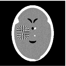
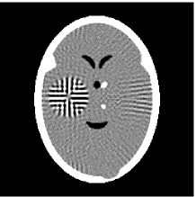
TV-S	TV-S
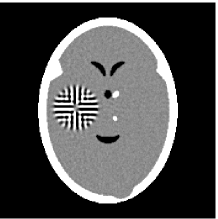
TV-PPS	TV-PPS

Figure 7: The reconstruction results of ghost phantom without noise. From left to right, the images in each row are reconstructed from 112, 82 projections.

Table 4: The MSE, number of iteration and running time(RT) of images in Fig. 7

Algorithm	TVS	TV-PPS	TVS	TV-PPS
projections	112	112	82	82
iterations	3	7	13	13
MSEs	0.0102	0.0080	0.0164	0.0158
RT(min)	2.0529	5.1975	10.382	9.1644

By comparing the images in Fig. 6, 7 and numbers in Table 3, 4, we can obtain the same conclusions that the proposed perturbation can not only improve qualities of reconstructed images, but also can accelerate the convergent speed. However, we can observe that the reconstruction images suffer from artifacts regardless of the classic and the proposed algorithm when the projections is inadequate.

4 Conclusion

We investigated an optimization-based method to determine the perturbation for superiorization algorithms. We analyzed the convergence of the proposed superiorization algorithm. Numerical experiments on different projection data for XCT image reconstruction were conducted to validate the good performance of the proposed perturbation. The experiments show that the perturbation determined by the proposed method can improve the quality of reconstructed images and convergent speed of the superiorization algorithms.

Since the superiorization methodology is a new algorithm for inverse problems, the superiorized iteration needs to be studied further from the mathematical theory and applications[12]. In the future, we will investigate acceleration methods and applications(parallel magnetic resonance imaging problem for instance) of superiorization algorithm.

References

- [1] G. T. Herman, Fundamentals of Computerized Tomography: Image Reconstruction from Projections. Springer, 2 ed., 2009.
- [2] F. Natterer and F. Wubbeling, Mathematical Methods in Image Reconstruction. Philadelphia: Society for Industrial and Applied Mathematics, 2001.
- [3] R. Gordon, R. Bender, and G. T. Herman, “Algebraic reconstruction techniques (ART) for three-dimensional electron microscopy and X-ray photography,” Journal of Theoretical Biology, vol. 29, no. 3, pp. 471–481, 1970.
- [4] A. R and C. Y, “Block-iterative projection methods for parallel computation of solutions to convex feasibility problems,” Linear Algebra and its Applications, vol. 120, p. 165 C75, 1989.
- [5] Y. Censor, T. Elfving, and G. T. Herman, “Averaging strings of sequential iterations for convex feasibility problems,” Studies in Computational Mathematics, no. 01, pp. 101–113, 2001.
- [6] L. A. Shepp and Y. Vardi, “Maximum likelihood restoration for emission tomography,” IEEE Transactions on Medical Imaging, vol. 1, no. 2, pp. 113–122, 1982.
- [7] M. Jiang and G. Wang, “Development of iterative algorithms for image reconstruction,” Journal of X-ray Science and Technology, vol. 10, no. 1/2, pp. 77–86, 2002.
- [8] E. Y. Sidky, C.-M. Kao, and X. Pan, “Accurate image reconstruction from few-views and limited-angle data in divergent-beam ct,” X-Ray Science and Technology, vol. 14, pp. 119–139, 2006.
- [9] E. Y. Sidky, J. H. Jorgensen, and X. Pan, “Convex optimization problem prototyping for image reconstruction in computed tomography with the chambolle-pock algorithm,” Physics in Medicien and Biology, vol. 57, no. 10, pp. 3065–3091, 2012.
- [10] G. T. Herman and R. Davidi, “Image reconstruction from a small number of projections,” Inverse Problems, vol. 24, no. 4, p. 045011, 2008.
- [11] R. Davidi, G. T. Herman, and Y. Censor, “Perturbation-resilient block-iterative projection methods with application to image reconstruction from projections.,” International Transactions in Operational Research, vol. 16, no. 4, pp. 505–524, 2009.
- [12] Y. Censor, R. Davidi, and G. T. Herman, “Perturbation resilience and superiozation of iterative algorithms,” Inverse Problems, vol. 26, no. 6, pp. 065008–065020, 2010.
- [13] L. Rudin, S. Osher, and E. Fatemi, “Nonlinear total variation based noise removal algorithms,” Physica D-nonlinear Phenomena, vol. 60, no. 1, pp. 259–268, 1992.
- [14] M. Lysaker, A. Lundervold, and X. Tai, “Noise removal using fourthorder partial differential equation with applications to medical magnetic resonance images in space and time,” IEEE Transactions on Image Processing, vol. 12, no. 12, p. 1579 C1590, 2003.
- [15] T. Chan, S. Esedoglu, and F. Park, “A fourth order dual method for staircase reduction in texture extraction and image restoration problems,” tech. rep., UCLA CAM Report, 2005.
- [16] D. Butnariu, R. Davidi, G. T. Herman, and I. G. Kazantsev, “Stable convergence behavior under summable perturbations of a class of projection methods for convex feasibility and optimization problems,” IEEE Journal of Selected Topics in Signal Processing, vol. 1, no. 4, pp. 540–547, 2008.
- [17] T. Nikazad, R. Davidi, and G. T. Herman, “Accelerated perturbation-resilient block-iterative projection methods with application to image reconstruction,” Inverse Problems, vol. 28, no. 3, p. 035005, 2012.
- [18] S. Luo and T. Zhou, “Superiorization of em algorithm and its application in singlephoton emission computed tomography(spect),” Inverse Problems and Imaging, vol. 8, no. 1, pp. 223–246, 2014.
- [19] W. Jin, Y. Censor, and M. Jiang, “A heuristic superiorization-like approach to bioluminescence tomography,” in Proceedings of the International Federation for Medical and Biological Engineering (IFMBE), vol. 39, 2012.
- [20] S. N. Penfold, R. W. Schulte, Y. Censor, and A. B. Rosenfeld, “Total variation superiorization schemes in proton computed tomography image reconstruction,” Medical Physics, vol. 37, pp. 5887–5895, 2010.
- [21] R. Davidi, R. W. Schulte, Y. Censor, and L. Xing, “Fast superiorization using a dual perturbation scheme for proton computed tomography,” Transactions of the American Nuclear Society, vol. 106, pp. 73–76, 2012.
- [22] D. Butnariu, R. Davidi, G. T. Herman, and I. G. Kazantsev, “Stable convergence behavior under perturbations of a class of projection methods for convex feasibility and optimization problems,” IEEE Journal of Selected Topic Signal Process, vol. 1, no. 4, pp. 540–547, 2007.
- [23] Y. Censor and A. J. Zaslavski, “Convergence and perturbation resilience of dynamic string-averaging projection methods,” Computational Optimization and Applications, vol. 54, no. 1, pp. 65–76, 2013.
- [24] W. Jin, Y. Censor, and M. Jiang, “Bounded perturbation resilience of projected scaled gradient methods,” Computational Optimization and Applications, vol. 63, no. 2, pp. 365–392, 2015.
- [25] A. Chambolle, “An algorithm for total variation minimization and applications,” Journal of Mathematical Imaging and Vision, vol. 20, no. 1, pp. 89–97, 2004.
- [26] T. Goldstein and S. Osher, “The split Bregman method for -regularized problems,” SIAM Journal on Imaging Sciences, vol. 2, no. 2, pp. 323–343, 2009.
- [27] C. A. Micchelli, L. Shen, and Y. Xu, “Proximity algorithms for image models: denoising,” Inverse Problems, vol. 27, no. 4, pp. 45009–45038(30), 2011.
- [28] W. Yin, S. Osher, D. Goldfarb, and J. Darbon, “Bregman iterative algorithms for -minimization with applications to compressed sensing,” Siam Journal on Imaging Sciences, 2008.
- [29] S. Boyd and L. Vandenberghe, Convex Optimization. New York: Cambridge University Press, 2004.
- [30] L. A. Shepp and B. F. Logan, “The fourier reconstruction of a head section,” IEEE Transactions on Nuclear Science, vol. NS-21, no. 3, pp. 21–43, 1974.
- [31] G. T. Herman, Image Reconstruction from Projections. New York, Academic: The Fundamentals of Computerized Tomography, 1980.