MCnet-16-35

Generation of central exclusive final statest1

Abstract

We present a scheme for the generation of central exclusive final states in the P YTHIA 8 program. The implementation allows for the investigation of higher order corrections to such exclusive processes as approximated by the initial-state parton shower in P YTHIA 8. To achieve this, the spin and colour decomposition of the initial-state shower has been worked out, in order to determine the probability that a partonic state generated from an inclusive sub-process followed by a series of initial-state parton splittings can be considered as an approximation of an exclusive colour- and spin-singlet process.

We use our implementation to investigate effects of parton showers on some examples of central exclusive processes, and find sizeable effects on di-jet production, while the effects on e.g. central exclusive Higgs production are minor.

1 Introduction

Figure 1: The basic diagram for a general central exclusive process $pp\to p+X+p$.

Compared to the fairly clean environment of $\mathrm{e}^{+}\mathrm{e}^{-}$ annihilation, proton collision events are in general very messy, especially at the LHC at high luminosity. Even at lower luminosity where pile-up events are absent, the existence of multiple soft interactions and initial-state parton showers means that any hard sub-process of interest will be obscured by soft and semi-hard hadrons smearing the measurements. However, for some rare events, a central colour-singlet hard sub-process may appear in complete isolation, with rapidity gaps on both sides stretching all the way out to the (quasi-) elastically scattered protons, giving a nice and clean environment to study its properties.

Such Central Exclusive Processes (CEPs) have been extensively studied in the so-called Durham formalism, first described by Khoze, Martin and Ryskin in Khoze:2000cy and reviewed in detail in Harland-Lang:2014lxa . The simplest such process is Higgs production, where two gluons in a colour- and spin-singlet state fuse together via a top-quark loop into a Higgs particle as outlined in figure 1. With an additional virtual exchange of a (semi-hard) gluon, the net colour exchange between the colliding protons can be zero and we may end up with a very simple and clean final state consisting only of two (quasi-) elastically scattered protons along the beam pipe and the Higgs decay products in the central rapidity region.

The formalism can be generalised to any colour-singlet hard sub-process, and the main ingredients to construct the amplitude is the matrix element for this sub-process and the so-called off-diagonal unintegrated parton densities. The latter can be interpreted as the amplitude related to the probability of finding gluons in a proton with equal but opposite transverse momentum, ${\bf q}_{\perp}$, and carrying energy fractions $x$ and $x^{\prime}$ each, one of which is being probed by a hard scale $\mu^{2}$. These densities also include a Sudakov form factor describing the probability that there is no additional initial-state radiation from the incoming gluon between the scales $q_{\perp}$ and $\mu$, which could destroy the rapidity gaps. Additional emissions below $q_{\perp}$ are then suppressed since they cannot resolve the individual colours of the two gluons. A third ingredient is the so-called soft survival probability which gives the probability that there are no additional soft or semi-hard interactions between the colliding protons which could destroy the rapidity gap.

Implementing the Durham formalism for CEP in an event generator is fairly straightforward since the final states are quite simple and clean. The cross section for any sub-process can be decomposed in a central exclusive luminosity function which is folded with a colour-singlet matrix element in a specific spin state. Several implementations have been made Monk:2005ji ; Boonekamp:2011ky ; Harland-Lang:2015cta , and in this paper will present yet another.

Our implementation is provided as an add-on to P YTHIA 8 Sjostrand:2014zea and is inspired by the observation that the Sudakov form factors in the off-diagonal unintegrated parton densities used within the Durham formalism can be interpreted in terms of no-emission probabilities in the parton shower language of P YTHIA 8.

In this way, we can reformulate the cross section for producing a CEP event in terms of a probability that a standard inclusive sub-process generated by P YTHIA 8 at some scale during the parton shower evolution is converted to a colour-singlet, and thereafter be considered a CEP event disallowing further initial-state shower splitting. The main advantage of this approach is that we actually are allowed to include initial-state shower splittings, and thus can approximately model higher order corrections to the original sub-process. In addition, we have the option of using the multiple interactions machinery of P YTHIA 8 to directly model soft survival probability as suggested in Cox:1999dw .

Consider, e.g., the central exclusive production of di-jets. We would start by generating the basic $2\to 2$ hard partonic scattering from the inclusive matrix element. We would then generate an initial-state parton emission from each of the incoming partons. This implicitly includes the probability that no emission has been made at a higher scale than the two generated splittings. If the colour and spin state of the original $2\to 2$ is consistent with a CEP, we basically take the ratio of the corresponding exclusive cross section and the one calculated with the inclusive matrix element, using the generated scales as factorisation scale. This gives us the probability to discard the generated splittings and continue the event as a CEP, or to keep the hardest emission and continue as a normal inclusive event.

If we continue the event as inclusive, we keep the hardest splitting and again generate one initial-state splitting from each side. Now that we have a three-parton final state which must be checked if it can be a candidate for CEP, but otherwise the procedure is repeated. It should be noted that P YTHIA 8 in general does not assign spin states to particles, so the procedure here also involves a spin decomposition of the parton splitting probabilities and the matrix elements to correctly get the probability for this to be a CEP. This will become cumbersome when we go up in parton multiplicity, but is still fairly straightforward.

The fact that we can stop the parton shower at any stage and check if we can convert the generated state exclusive, does not only mean that we can approximate higher order contributions from initial-state radiation. If we continue the parton shower evolution to low scales we are also able to investigate the transition region between the Durham formalism and the resolved Pomeron formalism Ingelman:1984ns which may produce similar final states.

The outline of this paper is as follows. First, we recapitulate the main features of the Durham formalism in section 2. Then we describe the different parts of our implementation in the P YTHIA 8 program, starting in section 3 with the reinterpretation of the exclusive luminosity function in terms of the parton shower no-emission probabilities, and followed by a description (section 4) of the spin and colour decomposition of a given partonic state generated by a parton shower from an inclusive hard matrix element. In section 5 we then present some proof-of-concept results for some sample processes before we conclude with a summary and outlook in section 6.

2 The Durham formalism

Within the Durham model, the amplitude, $\mathcal{A}$, of the central exclusive process in a $pp$ collision,

$$pp\to p+X+p,$$ (1)

can be written as

$$\frac{i\mathcal{A}}{s} = \int\frac{\pi^{2}\,\mathrm{d}^{2}{\bf q}\,\overline{\mathcal{M}}}{{\bf q}^{2}({\bf q}-{\bf p}_{1})^{2}(-{\bf q}-{\bf p}_{2})^{2}}$$ (2)

$$\times f_{g}(x_{1},x_{1}^{\prime},Q_{1}^{2},\mu^{2};t_{1})f_{g}(x_{2},x_{2}^{\prime},Q_{2}^{2},\mu^{2};t_{2})\,,$$

where the integration runs over the two-dimensional transverse momentum of the screening gluon ${\bf q}$ (Fig. 1). The transverse momenta of the outgoing protons are denoted as ${\bf p}_{1}$ and ${\bf p}_{2}$. The scales $Q_{1}^{2}$ and $Q_{2}^{2}$ are within Durham model Harland-Lang:2013ncy defined as

$$Q_{1}^{2} = \min\left[\,{\bf q}^{2},\,({\bf q}-{\bf p}_{1})^{2}\,\right],$$ (3)

$$Q_{2}^{2} = \min\left[\,{\bf q}^{2},\,(-{\bf q}-{\bf p}_{2})^{2}\,\right],$$ (4)

i.e. as the smaller of the virtualities of the screening gluon and the fusing gluon momenta related to the particular proton.

The proton form factors, $F_{N}$, are absorbed into off-diagonal unintegrated PDFs $f_{g}$. These PDFs are assumed to factorise as:

$$f_{g}(x,x^{\prime},Q^{2},\mu^{2};t)=f_{g}(x,x^{\prime},Q^{2},\mu^{2})F_{N}(t),$$ (5)

where $t_{1,2}\approx-{\bf p}_{1,2}^{2}$. The proton form factors in the simplest approach are $F_{N}(t)=\mathrm{e}^{bt/2}$, with $b\approx 4\,\mbox{GeV}^{-2}$. These off-diagonal unintegrated densities depend on the momentum fraction of the fusing (screening) gluon $x$ ($x^{\prime}$) and on two scales: the scale of the hard sub-process $\mu^{2}$; and the scale corresponding to the screening gluon transverse momentum $Q^{2}$.

The kinematic regime relevant for CEP is $Q/\sqrt{s}\sim x^{\prime}\ll x\sim M_{X}/\sqrt{s}$, which allows to integrate out the $x^{\prime}$-dependency of $f_{g}$ and express them using generalised gluon PDFs $H_{g}$ and the Sudakov factor $T_{M}$:

$$f_{g}(x,x^{\prime},Q^{2},\mu^{2}) =$$ (6)

$$\frac{\partial}{\partial\ln Q^{2}}\left[H_{g}\left(\frac{x}{2},\frac{x}{2};Q^{2}\right)\sqrt{T_{M}(Q^{2},\mu^{2})}\right]$$

The Sudakov factor $T_{M}$ describes the probability of no emission from the fusing gluons between scales $Q^{2}$ and $\mu^{2}$. It resumes singularities from virtual diagrams with soft or collinear emissions up to (modified) next-to-leading logarithmic accuracy and ensures that the integral (2) is finite, as the Sudakov factors exponentially suppress low ${\bf q}$ contribution.

$$T_{M}(Q^{2},\mu^{2}) = \exp\bigg{(}-\int_{Q^{2}}^{\mu^{2}}\frac{\mathrm{d}k^{2}}{k^{2}}\frac{\alpha_{s}(k^{2})}{2\pi}$$ (7)

$$\times\int_{0}^{1-\epsilon(k/M_{X})}\!\mathrm{d}z\,\left[zP_{gg}(z)+n_{f}P_{qg}(z)\right]\bigg{)}$$

In this expression both the splitting functions $P_{gg}$, $P_{qg}$ and the running of $\alpha_{s}$ are in the leading order form. The upper bound of the $z$ integration depends on the mass of the exclusive system which makes the Sudakov factor $T_{M}$ also $M_{X}$-dependent as indicated by the subscript, $M$.

The generalised PDF $H_{g}$ Harland-Lang:2013xba can be approximately calculated from the ordinary parton distribution function of gluon $g(x,Q^{2})$ using relation:

$$H_{g}\left(\frac{x}{2},\frac{x}{2};Q^{2}\right)=\frac{4}{\pi}\int_{\frac{x}{4}}^{1}\mathrm{d}y\;x\sqrt{y(1-y)}\;g\left(\frac{x}{4y},Q^{2}\right),$$ (8)

In a much used approximation the generalised PDF, $H_{g}$, is simply proportional to the conventional one

$$H_{g}\left(\frac{x}{2},\frac{x}{2};Q^{2}\right)=R_{g}\,x\,g(x,Q^{2}),$$ (9)

where the constant $R_{g}$ is about $1.3$ for LHC energies Harland-Lang:2013xba .

The sub-process amplitude $\mathcal{M}$ depends on transverse momenta of the fusing gluons ${\bf q}_{1}$ and ${\bf q}_{2}$

$${\bf q}_{1}={\bf q}-{\bf p}_{1}\qquad{\bf q}_{2}=-{\bf q}-{\bf p}_{2}$$ (10)

and on the $gg\to X$ vertex $V_{ij}^{ab}$ which is averaged over identical colour indexes $a=b$.

$$\mathcal{M}=\frac{2}{M_{X}^{2}}\frac{1}{N_{C}^{2}-1}\delta^{ab}q_{1}^{i}q_{2}^{j}V^{ab}_{ij}$$ (11)

The sub-process amplitude is typically known in the helicity basis. In this basis the vertex term $q_{1}^{i}q_{2}^{j}\,V^{aa}_{ij}$ takes form:

$$q_{1}^{i}q_{2}^{j}\,V^{aa}_{ij} =$$ (21)

$$=\left\{\begin{array}[]{ll}-\frac{1}{2}(q^{x}_{1}q^{x}_{2}+q^{y}_{1}q^{y}_{2})\times(A_{++}+A_{--})\\ -\frac{i}{2}(q^{x}_{1}q^{y}_{2}-q^{y}_{1}q^{x}_{2})\times(A_{++}-A_{--})\\ +\frac{1}{2}\left[(q^{x}_{1}q^{x}_{2}-q^{y}_{1}q^{y}_{2})+i(q^{x}_{1}q^{y}_{2}+q^{y}_{1}q^{x}_{2})\right]\times A_{-+}\\ +\frac{1}{2}\left[(q^{x}_{1}q^{x}_{2}-q^{y}_{1}q^{y}_{2})-i(q^{x}_{1}q^{y}_{2}+q^{y}_{1}q^{x}_{2})\right]\times A_{+-}\end{array}\right.$$

$$\equiv\left\{\begin{array}[]{ll}{\cal S}_{0^{+}}({\bf q}_{1},{\bf q}_{2})&\times(A_{++}+A_{--})\\ {\cal S}_{0^{-}}({\bf q}_{1},{\bf q}_{2})&\times(A_{++}-A_{--})\\ {\cal S}_{+2^{+}}({\bf q}_{1},{\bf q}_{2})&\times A_{-+}\\ {\cal S}_{-2^{+}}({\bf q}_{1},{\bf q}_{2})&\times A_{+-}\end{array}\right.,$$

where we have introduced the kinematic spin factors ${\cal S}_{J_{z}}({\bf q}_{1},{\bf q}_{2})$ for future reference with $q_{1}^{i}=q^{i}-p_{1}^{i}$ and $q_{2}^{i}=-q^{i}-p_{2}^{i}$ ($i=x,y$), and the amplitudes, e.g. $A_{++}$, depend on $M_{X}$, the momenta of outgoing particles, the helicities of outgoing particles as well as the helicities of incoming gluons (here both $+1$). The amplitudes also depend on the colours of the particles in the sub-process. Here, the amplitudes $A$ are the result of averaging over colour indexes of the incoming partons in such a way that the exclusive system is a colour singlet.

It is useful to note that in the collinear limit, where ${\bf q}_{1}=-{\bf q}_{2}={\bf q}$ the kinematic factors are simply:

$${\cal S}_{0^{+}}({\bf q},-{\bf q})=\frac{1}{2}{\bf q}^{2},\qquad{\cal S}_{0^{-}}({\bf q},-{\bf q})=0,$$

$$\mbox{and}\qquad{\cal S}_{\pm 2^{+}}({\bf q},-{\bf q})=-\frac{1}{2}{\bf q}^{2}\,\mathrm{e}^{\pm 2i\phi},$$ (22)

where the azimuthal angle of ${\bf q}$ was labelled as $\phi$. The state $J_{z}=0^{-}$ is trivially zero as a consequence of cross product of two collinear vectors. States $|J_{z}|=2$ become zero after integration over $\phi$ because the remaining part of (2) is $\phi$ independent in the collinear limit. Beyond such collinear limit also non spin-singlet states contribute to the cross section, but are suppressed as $\langle{\bf q}^{2}\rangle^{2}/\langle{\bf p}_{1,2}^{2}\rangle^{2}\sim 0.01$ with respect to the spin singlet term Harland-Lang:2015cta (if all helicity amplitudes, $A$, are of the same size).

Note that the formula (2) does not include a soft survival probability which cannot be calculated in a perturbative way. It reduces the CEP cross section at LHC by typically two orders of magnitude and can, e.g., be determined using the eikonal model Harland-Lang:2013xba ; Khoze:2014aca ; Khoze:2002nf .

3 Reinterpretation of the exclusive cross section

3.1 Prerequisites

In the following discussion it will be beneficial to reformulate the CEP amplitude of the Durham model into more straightforward form and rather work directly with the exclusive cross section $\sigma^{exc}$

$$\sigma^{exc} = \int\mathrm{d}y\,\mathrm{d}\ln M^{2}\mathrm{d}^{2}{{\bf p}_{1}}\mathrm{d}^{2}{\bf p}_{2}\,\mathrm{e}^{-b{\bf p}_{1}^{2}}\mathrm{e}^{-b{\bf p}_{2}^{2}}\frac{1}{64\pi^{2}}\frac{1}{2M^{2}}$$

$$\times \quad\bigg{|}\int\frac{\mathrm{d}^{2}{\bf q}\,\,q_{1}^{i}q_{2}^{j}\,V_{ij}^{aa}(M,w,\mu_{R}^{2})}{{\bf q}^{2}({\bf q}-{\bf p}_{1})^{2}(-{\bf q}-{\bf p}_{2})^{2}}$$

$$\times f_{g}^{M}(x_{1},x^{\prime}_{1},Q_{1}^{2},\mu_{F}^{2})f_{g}^{M}(x_{2},x^{\prime}_{2},Q_{2}^{2},\mu_{F}^{2})\;\bigg{|}^{2}\mathrm{d}\Sigma_{w}.$$

The variables $y$ and $M$ denote the rapidity and mass of the exclusive system and are related to the momenta fractions $x_{1}$ and $x_{2}$ by formulas

$$x_{1}=\frac{M}{\sqrt{s}}\;e^{y}\qquad x_{2}=\frac{M}{\sqrt{s}}\;e^{-y}.$$ (24)

The transverse momenta ${\bf p}_{1}$ and ${\bf p}_{2}$ of the scattered protons are assumed to be distributed according the simple one-channel model with the slope of the exponential equal to $b\sim 4\,\mbox{GeV}^{-2}$. The integration inside the absolute value is performed over transverse momentum ${\bf q}$ of the “screening” gluon. The other variables are recognised from the previous section. For completeness the dependency of the off-diagonal generalised PDFs on mass $M$ (via a Sudakov form factor) as well as the arguments of the $V_{ij}^{aa}$ are written explicitly. The kinematics of all outgoing particles of the exclusive system $X$ is denoted by $w$ and $\mathrm{d}\Sigma_{w}$ is the corresponding phase space element. The whole expression is integrated over phase space of these outgoing momenta $w$ which satisfy imposed kinematic cuts.

Inspired by a similar form of the derivative of the exponential function, we factorise the Sudakov factor in expression (6) in front of the bracket which leads to

$$f_{g}^{M}(x,x^{\prime},Q^{2},\mu_{F}^{2})=\sqrt{T_{M}(Q^{2},\mu_{F}^{2})}\;\phi_{M}(x,Q^{2}),$$ (25)

where the newly introduced modified PDF $\phi_{M}$ is defined as:

$$\phi_{M}(x,Q^{2}) = \bigg{[}\frac{\mathrm{d}H_{g}(\frac{x}{2},\frac{x}{2};Q^{2})}{\mathrm{d}\ln Q^{2}}$$

$$+\frac{\alpha_{s}(Q^{2})}{4\pi}H_{g}\left(\frac{x}{2},\frac{x}{2};Q^{2}\right)$$

$$\times\int_{0}^{1-\epsilon\left(\frac{Q}{M}\right)}\mathrm{d}z\left[zP_{gg}(z)+n_{f}(Q)P_{qg}(z)\right]\bigg{]}$$

In the text below, for simplicity, only the dominant spin singlet part will be considered and the following abbreviation is introduced:

$$\mathcal{D}^{2}_{1,2}\,{\bf q}=\frac{\mathrm{d}^{2}{\bf q}}{{\bf q}^{2}({\bf q}-{\bf p}_{1})^{2}(-{\bf q}-{\bf p}_{2})^{2}}({\bf q}-{\bf p}_{1})\cdot(-{\bf q}-{\bf p}_{2}),$$ (27)

where the indexes $1,2$ indicate the dependency of the differential on transverse momenta ${\bf p}_{1}$ and ${\bf p}_{2}$ and the dot represents the scalar product of two-dimensional vectors. In the collinear limit this differential simplifies to $-\mathrm{d}^{2}{\bf q}/{\bf q}^{4}$.

Using these notations and assumptions the formula (3.1) takes form:

$$\sigma^{exc} = \int\mathrm{d}y\,\mathrm{d}\ln M^{2}\mathrm{d}^{2}{{\bf p}_{1}}\mathrm{d}^{2}{\bf p}_{2}\,\mathrm{e}^{-b{\bf p}_{1}^{2}}\mathrm{e}^{-b{\bf p}_{2}^{2}}$$ (28)

$$\times\frac{1}{256\pi^{2}}\frac{1}{2M^{2}}\mathcal{D}^{2}_{1,2}\,{\bf q}\;\mathcal{D}^{2}_{1,2}\,{\bf q}^{\prime}$$

$$\times\phi_{M}(x_{1},Q_{1}^{2})\phi_{M}(x_{2},Q_{2}^{2})\phi_{M}(x_{1},Q_{1}^{\prime 2})\phi_{M}(x_{2},Q_{2}^{\prime 2})$$

$$\times T_{M}^{1/2}(Q_{1}^{2},\mu_{F}^{2})T_{M}^{1/2}(Q_{2}^{2},\mu_{F}^{2})T_{M}^{1/2}(Q_{1}^{\prime 2},\mu_{F}^{2})T_{M}^{1/2}(Q_{2}^{\prime 2},\mu_{F}^{2})$$

$$\times|A_{++}+A_{--}|^{2}\mathrm{d}\Sigma_{w},$$

where ${\bf q}^{\prime}$ is the transverse momentum of the screening gluon in the complex conjugate amplitude.

In the next step, the exclusive cross section (28) will be expressed as a product of the exclusive luminosity and the exclusive cross section. We define the spin-singlet colour-singlet cross section of hard sub-process as:

$$\sigma^{s}(w,\mu_{r}^{2})=\frac{1}{4}\frac{1}{64}\frac{1}{2M^{2}}\sum_{\lambda,j}\left|\sum_{a=1}^{8}\left(A_{++\to\lambda}^{aa\to j}+A_{--\to\lambda}^{aa\to j}\right)\right|^{2},$$ (29)

where the factor $1/4$ follows from the probability to have some particular helicity configuration of the incoming gluons and the coefficient $1/64$ has an analogous meaning for the colours. The term $1/2M^{2}$ represents the “flux factor”. The symmetrisation factor, $N_{s}$, important if identical particles occur in the final state, is assumed to be incorporated in the amplitudes $A$, i.e. amplitudes are scaled by $1/\sqrt{N_{s}}$. Letters $\lambda$ and $j$ denote all possible helicity and colour configurations of the exclusive system.

The exclusive luminosity which corresponds to the exclusive cross section of the hard sub-process (29) is:

$$L_{exc}(M,y,\mu_{F}^{2}) =$$

$$\times\int\frac{1}{\pi^{2}}\mathrm{d}^{2}{{\bf p}_{1}}\mathrm{d}^{2}{\bf p}_{2}\,\mathrm{e}^{-b{\bf p}_{1}^{2}}\,\mathrm{e}^{-b{\bf p}_{2}^{2}}\,\mathcal{D}^{2}_{1,2}\,{\bf q}\;\mathcal{D}^{2}_{1,2}\,{\bf q}^{\prime}$$

$$\times\phi_{M}(x_{1},Q_{1}^{2})\phi_{M}(x_{2},Q_{2}^{2})\phi_{M}(x_{1},Q_{1}^{\prime 2})\phi_{M}(x_{2},Q_{2}^{\prime 2})$$

$$\times T_{M}^{1/2}(Q_{1}^{2},\mu_{F}^{2})T_{M}^{1/2}(Q_{2}^{2},\mu_{F}^{2})$$

$$\times T_{M}^{1/2}(Q_{1}^{\prime 2},\mu_{F}^{2})T_{M}^{1/2}(Q_{2}^{\prime 2},\mu_{F}^{2}).$$

In the collinear limit, where ${\bf p}_{1}$ and ${\bf p}_{2}$ are neglected with respect to ${\bf q}$ and ${\bf q}^{\prime}$, the luminosity can be integrated over ${\bf p}_{1}$ and ${\bf p}_{2}$ and over the azimuthal angles of ${\bf q}$ and ${\bf q}^{\prime}$ which leads to:

$$L_{exc}(M,y,\mu_{F}^{2}) = \frac{\pi^{2}}{b^{2}}\int\!\frac{\mathrm{d}q^{2}}{q^{4}}\frac{\mathrm{d}q^{\prime 2}}{q^{\prime 4}}$$

$$\times\phi_{M}(x_{1},q^{2})\phi_{M}(x_{2},q^{2})\phi_{M}(x_{1},q^{\prime 2})\phi_{M}(x_{2},q^{\prime 2})$$

$$\times T_{M}(q^{2},\mu_{F}^{2})T_{M}(q^{\prime 2},\mu_{F}^{2})$$

$$L_{exc}(M,y,\mu_{F}^{2}) =$$

$$\frac{\pi^{2}}{b^{2}}\bigg{|}\int\frac{\mathrm{d}\ln q^{2}}{q^{2}}\phi_{M}(x_{1},q^{2})\phi_{M}(x_{2},q^{2})\;T_{M}(q^{2},\mu_{F}^{2})\bigg{|}^{2}$$

The integrand in (3.1) is fairly flat if considered as a function of $1/q^{2}$ and $1/q^{\prime 2}$ which makes these variables suitable for Monte Carlo integration, especially because $\mathrm{d}(1/q^{2})=-\mathrm{d}q^{2}/q^{4}$.

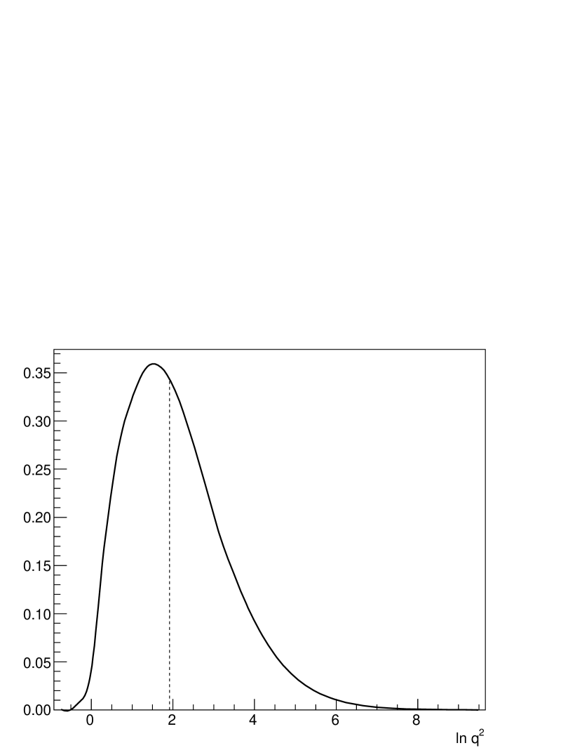
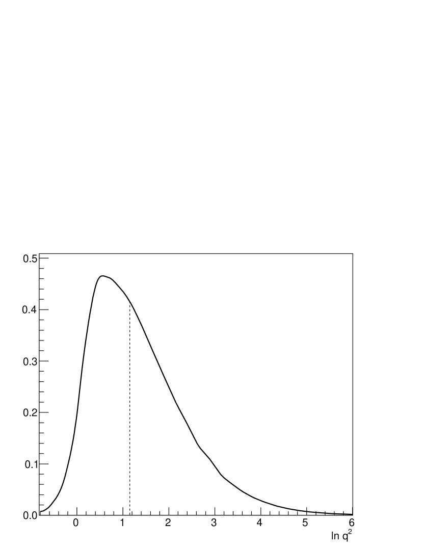
Figure 2: Integrand of formula (3.1) for Higgs production at LHC, $\sqrt{s}=13\,\mbox{TeV}$ and $\mu_{F}=125\,\mbox{GeV}$ (left), and for di-jet production at Tevatron, $\sqrt{s}=1.96\,\mbox{TeV}$ and $\mu_{F}=25\,\mbox{GeV}$ (right). The dashed lines depict the medians of the distributions, which are $2.6\,\mbox{GeV}$ for LHC and $1.8\,\mbox{GeV}$ for Tevatron. We calculated the generalised gluon PDF $H_{g}$ from MMHT2014 LO PDF using formula (8).

The integrand in (3.1) is shown in Fig. 2 for $\ln q^{2}$ as an integration variable. For calculating of the exclusive luminosity the upper limit of integration is set to the factorisation scale $\mu_{F}$, nevertheless the integrand is typically negligible in the high $q$ region. Whereas it dominates for $q$ of $2-3\,\mbox{GeV}$ in case of LHC Higgs production and for even smaller values ($1-2\,\mbox{GeV}$) in case of di-jet production at Tevatron. Values below the starting scale $q_{0}=1\,\mbox{GeV}$ of MMHT2014 LO PDF Harland-Lang:2014zoa can be extracted using a backward DGLAP evolution Botje:2010ay . In reality, it was argued in Khoze:2004yb that for $q\lesssim 0.85\,\mbox{GeV}$ the gluon propagator would be modified by non-perturbative dynamics which effectively suppress such low $q$ contributions. Rather than a sharp cut-off, the damped gluon PDF Harland-Lang:2015cta is used to calculate $\phi_{M}$ below $q_{0}$ in order to suppress the region of low transverse momentum:

$$g(x,q)=g(x,q_{0})\left(\frac{q^{2}}{q_{0}^{2}}\right)^{2+(a_{1}-2)(q^{2}/q_{0}^{2})+a_{2}(q^{2}/q_{0}^{2})^{2}}$$

$$\text{for}\quad q<q_{0}$$ (33)

The coefficients $a_{1,2}$ are chosen in such a way that the function is smooth in $q_{0}$ up to the second derivative.

Finally, the CEP cross section expressed as a convolution of the exclusive luminosity (3.1) and the exclusive cross section of the hard sub-process (29) takes from

$$\sigma^{exc}=\int\mathrm{d}y\,\mathrm{d}\ln M^{2}\;L_{exc}(M,y,\mu_{F}^{2})\,\sigma^{s}(M,w,\mu_{R}^{2})\,\mathrm{d}\Sigma_{w},$$ (34)

in analogy with the formula formula for the inclusive cross section

$$\sigma^{inc}=\int\mathrm{d}y\,\mathrm{d}\ln M^{2}\;L_{inc}(M,y,\mu_{F}^{2})\,\sigma^{i}(M,w,\mu_{R}^{2})\,\mathrm{d}\Sigma_{w},$$ (35)

where the inclusive luminosity $L_{inc}$ is

$$L_{inc}(M,y,\mu_{F}^{2})=x_{1}g(x_{1},\mu_{F}^{2})\;x_{2}g(x_{2},\mu_{F}^{2}).$$ (36)

3.2 Screening gluons in the P YTHIA 8 interleaved parton shower

The way parton showers are included in P YTHIA 8 is through an interleaved process where we normally have three competing processes, which we will denote ISR, FSR and MPI. ISR is an initial-state splitting where one of the incoming partons to the hard sub-process is evolved to lower scale and higher energy fraction, by emitting a parton into the final state; FSR is the final-state splitting of a parton in the final state; while MPI is the appearance of an additional parton–parton interaction. All of these occur at decreasing scale, where the highest scale is given by the kinematics of the hard sub-process. In each step in the shower we then pick a process which has a lower scale than the previous one, and the factorisation property of the no-emission probability means that we can generate one of each of the possible processes independently and simply pick the one which yielded the highest scale in each step.

For simplicity we will here only consider the ISR, concentrating on the initial-state $g\to gg$ splittings, and show how we can reinterpret the formula for CEP as an extra process in the interleaved shower, which transforms an inclusive event into an exclusive one.

First, let’s consider the inclusive processes with no emission from the space-like shower between scales $\mu^{2}$ and $\mu_{F}^{2}$. The scale $\mu_{F}^{2}$ is considered as a starting scale of the backward space-like parton shower. The cross section for such processes take form:

$$\sigma^{inc}(\mu^{2}) = \int\mathrm{d}y\,\mathrm{d}\ln M^{2}\;L_{inc}(M,y,\mu_{F}^{2})$$

$$T_{M}^{x_{1}}(\mu^{2},\mu_{F}^{2})T_{M}^{x_{2}}(\mu^{2},\mu_{F}^{2})\sigma^{i}(M,w,\mu_{r}^{2})\,\mathrm{d}\Sigma_{w},$$

where $T_{M}^{x}$ is the no-emission probability, quantifying the probability that no extra emission from parton are present between two given scales, if the higher scale is taken as a reference. This no-emission term is used in the backward evolution of the space-like showers in Pythia and, for the case of an incoming gluon, it is defined as:

$$T_{M}^{x}(q_{1}^{2},q_{2}^{2}) = \exp\bigg{(}-\int_{q_{1}^{2}}^{q_{2}^{2}}\frac{\mathrm{d}q^{2}}{q^{2}}\frac{\alpha_{s}(q^{2})}{2\pi}$$

$$\times\sum_{a}\int_{x}^{1-\epsilon\left(\frac{q}{M}\right)}\frac{\mathrm{d}z}{z}\frac{f_{a}(\frac{x}{z},q^{2})}{g(x,q^{2})}P_{a\to g}(z)\bigg{)},$$

where the sum runs over gluons and all possible flavours of quarks and anti-quarks. It can be shown that these no-emission probabilities are linked to the standard Sudakov form factors by the relation Krauss:2002up ; Lavesson:2005xu :

$$T_{M}^{x}(q_{1}^{2},q_{2}^{2})=\frac{g(x,q_{1}^{2})}{g(x,q_{2}^{2})}T_{M}(q_{1}^{2},q_{2}^{2})$$ (39)

The cross section $\sigma^{inc}$, differential in the variable $\ln\mu^{2}$, corresponding to the scale of the first parton shower emission is:

$$\frac{\mathrm{d}\sigma^{inc}(\mu^{2})}{\mathrm{d}\ln\mu^{2}}=\int\mathrm{d}y\,\mathrm{d}\ln M^{2}\;L_{inc}(M,y,\mu_{F}^{2})\times$$

$$\frac{\mathrm{d}}{\mathrm{d}\ln\mu^{2}}\Big{(}T_{M}^{x_{1}}(\mu^{2},\mu_{F}^{2})T_{M}^{x_{2}}(\mu^{2},\mu_{F}^{2})\Big{)}$$

$$\sigma^{i}(M,w,\mu_{R}^{2})\,\mathrm{d}\Sigma_{w}$$ (40)

Employing the relation (39) the derivative of the no-emission probabilities can be expressed using the Sudakov factors only:

$$\frac{\mathrm{d}}{\mathrm{d}\ln\mu^{2}}\Big{(}T_{M}^{x_{1}}(\mu^{2},\mu_{F}^{2})T_{M}^{x_{2}}(\mu^{2},\mu_{F}^{2})\Big{)}=T_{M}(\mu^{2},\mu_{F}^{2})^{2}$$ (41)

$$\times\frac{\tilde{g}(x_{1},\mu^{2})x_{2}g(x_{2},\mu^{2})+x_{1}g(x_{1},\mu^{2})\tilde{g}(x_{2},\mu^{2})}{x_{1}g(x_{1},\mu_{F}^{2})x_{2}g(x_{2},\mu_{F}^{2})},$$

where the newly defined distribution function $\tilde{g}$ is:

$$\tilde{g}(x,\mu^{2}) = x\frac{\partial g(x,\mu^{2})}{\partial\ln q^{2}}+xg(x,\mu^{2})$$

$$\times\,\frac{\alpha_{s}(\mu^{2})}{2\pi}\int_{0}^{1-\epsilon(\mu/M)}\mathrm{d}z\left[zP_{gg}(z)+n_{f}(\mu)P_{qg}(z)\right]$$

It allows to re-express the differential cross section (40) using the standard Sudakov form factors:

$$\frac{\mathrm{d}\sigma^{inc}(\mu^{2})}{\mathrm{d}\ln\mu^{2}} = \int\mathrm{d}y\,\mathrm{d}\ln M^{2}$$

$$\Big{[}\tilde{g}(x_{1},\mu^{2})x_{2}g(x_{2},\mu^{2})+x_{1}g(x_{1},\mu^{2})\tilde{g}(x_{2},\mu^{2})\Big{]}$$

$$\qquad\quad\times\;T_{M}(\mu^{2},\mu_{F}^{2})^{2}\,\sigma^{i}(M,w,\mu_{R}^{2})\,\mathrm{d}\Sigma_{w}$$

The inclusive cross section is then simply:

$$\sigma^{inc}=\int^{\mu_{F}^{2}}\mathrm{d}\ln\mu^{2}\,\frac{\mathrm{d}\sigma^{inc}(\mu^{2})}{\mathrm{d}\ln\mu^{2}},$$ (44)

where the lower integration limit is assumed to be so small that the Sudakov factor between this limit and $\mu_{F}^{2}$ is close to zero.

We can now apply a similar procedure to the exclusive cross section where the variable $\mu^{2}$ is now interpreted as the minimal transverse momentum of the screening gluons exchanged during the interaction. Let’s define:

$$\frac{\mathrm{d}L_{exc}(M,y,\mu_{F}^{2},\mu^{2})}{\mathrm{d}\ln\mu^{2}} = \frac{\mathrm{d}}{\mathrm{d}\ln\mu^{2}}\frac{\pi^{2}}{b^{2}}$$

$$\times\;\bigg{|}\int_{\mu^{2}}^{\mu_{F}^{2}}\mathrm{d}\ln q^{2}\;\frac{1}{q^{2}}\phi_{M}(x_{1},q^{2})\phi_{M}(x_{2},q^{2})\;T_{M}(q^{2},\mu_{F}^{2})\bigg{|}^{2}$$

$$=-\frac{\pi^{2}}{b^{2}}\frac{2}{\mu^{2}}\phi_{M}(x_{1},\mu^{2})\phi_{M}(x_{2},\mu^{2})T_{M}(\mu^{2},\mu_{F}^{2})^{2}\times$$

$$\times\int_{\mu^{2}}^{\mu_{F}^{2}}\frac{\mathrm{d}\ln q^{2}}{q^{2}}\phi_{M}(x_{1},q^{2})\phi_{M}(x_{2},q^{2})\frac{1}{T_{M}(\mu^{2},q^{2})}$$

Then the derivative of the exclusive cross section according to this variable is simply:

$$\frac{\mathrm{d}\sigma^{exc}(\mu^{2})}{\mathrm{d}\ln\mu^{2}} = \int\mathrm{d}y\,\mathrm{d}\ln M^{2}$$ (46)

$$\frac{\mathrm{d}L_{exc}(M,y,\mu_{F}^{2},\mu^{2})}{\mathrm{d}\ln\mu^{2}}\,\sigma^{s}(M,w,\mu_{R}^{2})\,\mathrm{d}\Sigma_{w}.$$

The ratio of the integrands in eqs. (46) and (3.2) defines the exclusive probability

$$p_{exc} = \frac{-\frac{1}{T_{M}(\mu^{2},\mu_{F}^{2})^{2}}\frac{\mathrm{d}L_{exc}(M,y,\mu_{F}^{2},\mu^{2})}{\mathrm{d}\ln\mu^{2}}}{\left(\tilde{g}(x_{1},\mu^{2})x_{2}g(x_{2},\mu^{2})+x_{1}g(x_{1},\mu^{2})\tilde{g}(x_{2},\mu^{2})\right)}$$ (47)

$$\times\frac{\sigma^{s}(M,w,\mu_{R}^{2})}{\sigma^{i}(M,w,\mu_{R}^{2})}.$$

This means that we now have for each step in the interleaved shower a probability for a given partonic state to become exclusive by the exchange of a screening gluon. The physical picture is the same as in the Durham model, in that a screening gluon with low transverse momentum cannot affect the colour structure of an emission at a higher scale. It also has the nice property that we become somewhat insensitive to the low transverse momentum behaviour of the parton densities in the integral of the exclusive luminosity.

There is, however, a problem with this approach, in that the $p_{exc}$ is very peaked at small $\mu$, making the generation of the exclusive events very inefficient. Although a weighting procedure could be applied, it would be difficult to incorporate into the current framework of P YTHIA 8. For the purpose of this paper, we have therefore chosen to implement a simpler procedure.

3.3 A simpler approach

Instead of adding the exchange of a screening gluon as an extra process in the interleaved shower, we simply calculate before each shower step, if given state should be made exclusive, using the probability

$$p^{\prime}_{exc}=\frac{L_{exc}(M,y,\mu^{2})}{L_{inc}(M,y,\mu^{2})}\;\frac{\sigma^{\prime s}(M,w,\mu_{R}^{2})}{\sigma^{\prime i}(M,w,\mu_{R}^{2})},$$ (48)

where $\mu^{2}$ is the scale of the latest emission. We note that the integration in $L_{exc}$ now goes down to very low transverse momenta, but it turns out that the results are the same as in the more complicated approach above.

The modified cross section $\sigma^{\prime i}$ is defined as:

$$\sigma^{\prime i}=P_{n}(z_{n})P_{n-1}(z_{n-1})\ldots P_{2}(z_{2})P_{1}(z_{1})\sigma^{i},$$ (49)

where the $P_{i}$ splitting functions in principle could be either initial- or final-state splittings. For modified singlet sub-process cross section the definition is the same, only the formula is corrected for the fact that the incoming gluons are in colour and spin singlet state which, for example, makes $H+\mathrm{jet}$ exclusive cross section equal to zero. Note that for calculation of the modified singlet cross section, not only classical matrix element squared but also amplitudes for all possible helicity configuration must be known. The procedure for calculating $\sigma^{\prime}_{s}$ will be provided in the next section.

The full procedure would be to start the generation of an inclusive process in P YTHIA 8 and calculate the probability in (48) of that process being exclusive. Then, after each ISR or FSR step in the interleaved shower, we would again check if the current state can be made exclusive by (48). If the event is to be considered to be exclusive we would rearrange the colour flow accordingly and insert the quasi-elastically scattered protons, but let the shower continue without the ISR process.

Note that the soft survival probability, which we have so far left out of the exclusive luminosity function, corresponds exactly to the probability of having no additional multi-parton interactions, so any MPI in the interleaved shower (before or after the event has been made exclusive) will mean that the event will stay inclusive.

To make the generation of exclusive events more efficient we have here decided to simplify the procedure even more. A final-state emission does not modify the parton densities used in the luminosity functions, and although they may affect the exclusive cross section, we have here decided to leave them out and generate them separately. Also the calculation of the soft survival probability by vetoing any exclusive event in case the shower gives a MPI is extremely inefficient, and we instead calculate that separately and simply multiply the inclusive cross section with that factor. It should be noted that using the MPI model in P YTHIA 8 presented in Cox:1999dw has not been carefully investigated. It has the interesting feature that the probability for additional scattering depends on the hardness of the primary scattering, since harder processes have larger overlap (smaller impact parameter). It also has a natural dependence on the collision energy. The downside is that it is sensitive to the soft behaviour of MPI model and may vary strongly between different tunings of the parameters. In this paper we will simply use the default tune in P YTHIA 8 and postpone a proper investigation of the procedure to a future publication.

In the end, the procedure will look as follows:

1. Generate the hard sub-process of interest in P YTHIA 8, use the standard inclusive cross section.

2. Use only the initial-state shower in P YTHIA 8.

3. Before generating the next initial-state emission, make the event exclusive with the probability in (48).

4. If the event is made exclusive, switch off the initial-state cascade, rearrange colours, remove the proton remnants, insert the scattered protons and continue with final-state radiation from the exclusive state.

5. If the event stays inclusive, generate the next initial-state emission (continue with step 3).

As an alternative, to enable detailed studies of the exclusive processes we will below also use a procedure where we study a specific number of initial-state splittings or only initial-state splittings above a certain scale, $\mu_{exc}$, in which case we run the initial state shower without modification to get the desired states and only afterwards decide if the states should become exclusive.

This approach is efficient if the ratio $\frac{\sigma^{\prime s}}{\sigma^{\prime i}}$ does not heavily depend on the number of emissions. This is normally the case for higher emission multiplicities in contrast the first few emissions where the interference effects play a role. In the program both approaches are implemented and we use each of them in such a frequency so that the event weights variation is minimal.

3.4 Modified luminosity for all possible helicity configurations

Before proceeding to calculate $\sigma^{\prime s}$ in (48) we have to generalise the expression to include all possible helicity combinations contributing to the exclusive production. First, we define four kinds of the “luminosity amplitudes”, $\mathcal{L}^{(J_{z})}$, for $J_{z}=\{0^{+},0^{-},+2^{+},-2^{+}\}$, using the notation in (21):

$$\mathcal{L}^{(J_{z})} = \int\frac{\mathrm{d}^{2}{\bf q}\quad 2{\cal S}_{J_{z}}({\bf q}_{1},{\bf q}_{2})}{{\bf q}^{2}({\bf q}-{\bf p}_{1})^{2}(-{\bf q}-{\bf p}_{2})^{2}}$$

$$\phi_{M}(x_{1},Q_{1}^{2})\phi_{M}(x_{2},Q_{2}^{2})T_{M}^{1/2}(Q_{1}^{2},\mu_{F}^{2})T_{M}^{1/2}(Q_{2}^{2},\mu_{F}^{2})$$

For the future use, it is more convenient to work with $\mathcal{L}$ directly related to some particular helicity configuration of the partons entering to the hard sub-process. Let’s define

$$\mathcal{L}^{++} = \mathcal{L}^{(0^{+})}+\mathcal{L}^{(0^{-})},\quad\mathcal{L}^{--}=\mathcal{L}^{(0^{+})}-\mathcal{L}^{(0^{-})},$$ (51)

$$\mathcal{L}^{-+} = \mathcal{L}^{(+2^{+})},\qquad\qquad\mathcal{L}^{+-}=\mathcal{L}^{(-2^{+})}.$$ (52)

These relations allow us to rewrite the CEP cross section (3.1) as:

$$\sigma^{exc} = \int\mathrm{d}y\,\mathrm{d}\ln M^{2}\,\mathrm{d}^{2}{{\bf p}_{1}}\mathrm{d}^{2}{\bf p}_{2}\,\mathrm{e}^{-b{\bf p}_{1}^{2}}\mathrm{e}^{-b{\bf p}_{2}^{2}}\frac{1}{256\pi^{2}}\frac{1}{2M^{2}}\times$$ (53)

$$\times \sum_{\lambda,j}\Bigg{|}\sum_{a=1}^{8}\bigg{(}\mathcal{L}^{++}A_{++\to\lambda}^{aa\to j}+\mathcal{L}^{+-}A_{+-\to\lambda}^{aa\to j}+$$

$$\qquad\;+\mathcal{L}^{-+}A_{-+\to\lambda}^{aa\to j}+\mathcal{L}^{--}A_{--\to\lambda}^{aa\to j}\bigg{)}\Bigg{|}^{2}\mathrm{d}\Sigma_{w},$$

where $j$ and $\lambda$ denotes the colour state and helicity state of all final state particles of the hard sub-process. The index $i$ denotes the colour of the fusing gluons.

Finally, it is possible to formally factorise the cross section formula into process independent luminosity part and the cross section part:

$$\sigma^{exc} = \int\mathrm{d}y\,\mathrm{d}\ln M^{2}$$ (54)

$$\int\frac{1}{\pi^{2}}\,\mathrm{d}^{2}{{\bf p}_{1}}\mathrm{d}^{2}{\bf p}_{2}\,\mathrm{e}^{-b{\bf p}_{1}^{2}}\mathrm{e}^{-b{\bf p}_{2}^{2}}\sum_{\begin{subarray}{c}\lambda_{l}\lambda_{r}\\ \lambda^{\prime}_{l}\lambda^{\prime}_{r}\end{subarray}}\mathcal{L}^{\lambda_{l}\lambda_{r}}\mathcal{L}^{*\lambda^{\prime}_{l}\lambda^{\prime}_{r}}$$

$$\times \frac{1}{512M^{2}}\sum_{\begin{subarray}{c}\lambda,j\\ aa^{\prime}\end{subarray}}A_{\lambda_{l}\lambda_{r}\to\lambda}^{aa\to j}A_{\lambda^{\prime}_{l}\lambda^{\prime}_{r}\to\lambda}^{*a^{\prime}a^{\prime}\to j}\;\mathrm{d}\Sigma_{w}$$

$$\equiv \int\mathrm{d}y\,\mathrm{d}\ln M^{2}\,\,L^{exc}\!\left(\begin{subarray}{c}\lambda_{l}\lambda_{r}\\ \lambda^{\prime}_{l}\lambda^{\prime}_{r}\end{subarray}\right)\,\sigma^{s}\!\left(\begin{subarray}{c}\lambda_{l}\lambda_{r}\\ \lambda^{\prime}_{l}\lambda^{\prime}_{r}\end{subarray}\right)\,\mathrm{d}\Sigma_{w},$$

where there is an implicit summation in the last expression over all four helicity indices, and the generalised colour singlet cross section $\sigma^{s}$ incorporates the normalisation factor $\frac{1}{512M^{2}}$. The origin of this factor is explained below equation (29). Notice, that the cross section formula (54) is a direct generalisation of relation (34), where only the spin singlet component was considered.

A more general expression for the probability $p_{exc}$ of event being exclusive is then

$$p_{exc}=\frac{L^{exc}\!\left(\begin{subarray}{c}\lambda_{l}\lambda_{r}\\ \lambda^{\prime}_{l}\lambda^{\prime}_{r}\end{subarray}\right)\,\sigma^{\prime s}\!\left(\begin{subarray}{c}\lambda_{l}\lambda_{r}\\ \lambda^{\prime}_{l}\lambda^{\prime}_{r}\end{subarray}\right)}{L^{inc}\,\sigma^{\prime i}},$$ (55)

where the modified inclusive cross section $\sigma^{\prime i}$ which incorporates the splitting functions is defined by formula (49), whereas the corresponding cross section $\sigma^{\prime s}$ will be derived in the next section. Both luminosities are evaluated at scale of the latest initial-state emission.

4 Approximation of matrix elements using shower splittings

To calculate the central exclusive cross section, the amplitude for every helicity and colour combination of the studied sub-process must be known, rather than the spin- and colour-averaged sub-process cross section. For $2\to 2$ processes the amplitude $A^{\lambda_{l1}\lambda_{r1}\to\lambda_{3}\lambda_{4}}_{a_{l1}a_{r1}\to x_{3}x_{4}}$ depends on the helicities of the incoming ($\lambda_{l1},\lambda_{r1}$) and outgoing particles ($\lambda_{3},\lambda_{4}$) as well as on the colours of the corresponding particles $a_{l1}$, $a_{r1}$, $x_{3}$, $x_{4}$. The additional dependency on particle momenta is not written out explicitly.

It is useful to introduce the “generalised cross section” $\sigma$ of the hard sub-process:

$$\sigma\left(\begin{subarray}{c}a_{l1}a_{r1}\\ a^{\prime}_{l1}a^{\prime}_{r1}\end{subarray}\middle|\begin{subarray}{c}\lambda_{l1}\lambda_{r1}\\ \lambda^{\prime}_{l1}\lambda^{\prime}_{r1}\end{subarray}\right) =$$

$$\frac{1}{512M^{2}}\sum_{\begin{subarray}{c}x_{3}x_{4}\\ \lambda_{3}\lambda_{4}\end{subarray}}A^{\lambda_{l1}\lambda_{r1}\to\lambda_{3}\lambda_{4}}_{a_{l1}a_{r1}\to x_{3}x_{4}}\;\left(A^{\lambda^{\prime}_{l1}\lambda^{\prime}_{r1}\to\lambda_{3}\lambda_{4}}_{a^{\prime}_{l1}a^{\prime}_{r1}\to x_{3}x_{4}}\right)^{*}$$

which is summed over helicities and colours of the final state particles but not over initial-state one. Moreover, the colour and helicity indexes of the incoming particles are in general considered to be different for the amplitude and its complex conjugated. The generalisation of this cross section to $2\to n$ processes is straightforward.

Knowing the generalised cross section, the inclusive cross section takes the form:

$$\sigma^{inc}=\sum_{\begin{subarray}{c}\lambda_{l1}\lambda_{r1}\\ \lambda^{\prime}_{l1}\lambda^{\prime}_{r1}\end{subarray}}\delta_{\lambda_{l1}\lambda^{\prime}_{l1}}\delta_{\lambda_{r1}\lambda^{\prime}_{r1}}\sum_{\begin{subarray}{c}a_{l1}a_{r1}\\ a^{\prime}_{l1}a^{\prime}_{r1}\end{subarray}}\delta_{a_{l1}a^{\prime}_{l1}}\delta_{a_{r1}a^{\prime}_{r1}}$$

$$\times\;\sigma\left(\begin{subarray}{c}a_{l1}a_{r1}\\ a^{\prime}_{l1}a^{\prime}_{r1}\end{subarray}\middle|\begin{subarray}{c}\lambda_{l1}\lambda_{r1}\\ \lambda^{\prime}_{l1}\lambda^{\prime}_{r1}\end{subarray}\right),$$ (57)

where the nominal and complex conjugate indexes were put to be equal by means of delta functions.

The colour singlet spin singlet cross section $\sigma^{S(0^{+})}$ is obtained by an analogous formula (imposing “left” and “right” colours and helicities to be identical):

$$\sigma^{S(0^{+})}=\sum_{\begin{subarray}{c}\lambda_{l1}\lambda_{r1}\\ \lambda^{\prime}_{l1}\lambda^{\prime}_{r1}\end{subarray}}\delta_{\lambda_{l1}\lambda_{r1}}\delta_{\lambda^{\prime}_{l1}\lambda^{\prime}_{r1}}\sum_{\begin{subarray}{c}a_{l1}a_{r1}\\ a^{\prime}_{l1}a^{\prime}_{r1}\end{subarray}}\delta_{a_{l1}a_{r1}}\delta_{a^{\prime}_{l1}a^{\prime}_{r1}}$$

$$\times\;\sigma\left(\begin{subarray}{c}a_{l1}a_{r1}\\ a^{\prime}_{l1}a^{\prime}_{r1}\end{subarray}\middle|\begin{subarray}{c}\lambda_{l1}\lambda_{r1}\\ \lambda^{\prime}_{l1}\lambda^{\prime}_{r1}\end{subarray}\right),$$ (58)

Or using another notation:

$$\sigma^{S(0^{+})}=\sigma^{s}\left(\begin{subarray}{c}++\\ ++\end{subarray}\right)+\sigma^{s}\left(\begin{subarray}{c}--\\ --\end{subarray}\right)+\sigma^{s}\left(\begin{subarray}{c}++\\ --\end{subarray}\right)+\sigma^{s}\left(\begin{subarray}{c}--\\ ++\end{subarray}\right),$$ (59)

where the summation over helicities is made explicit and the generalised colour singlet cross section $\sigma^{s}$, firstly used in (54), is:

$$\sigma^{s}\left(\begin{subarray}{c}\lambda_{l1}\lambda_{r1}\\ \lambda^{\prime}_{l1}\lambda^{\prime}_{r1}\end{subarray}\right)=\sum_{\begin{subarray}{c}a_{l1}a_{r1}\\ a^{\prime}_{l1}a^{\prime}_{r1}\end{subarray}}\delta_{a_{l1}a_{r1}}\delta_{a^{\prime}_{l1}a^{\prime}_{r1}}\;\;\sigma\left(\begin{subarray}{c}a_{l1}a_{r1}\\ a^{\prime}_{l1}a^{\prime}_{r1}\end{subarray}\middle|\begin{subarray}{c}\lambda_{l1}\lambda_{r1}\\ \lambda^{\prime}_{l1}\lambda^{\prime}_{r1}\end{subarray}\right).$$ (60)

The aim of the following sections is to derive an approximative form of the generalised cross section for the case where we have initial-state parton shower splittings from the left and right incoming partons. These emissions are assumed to be strongly ordered in their $p_{\perp}$.

To be specific, let’s consider the gluon emission from the “left” incoming parton. The new generalised cross section will then take the form:

$$\sigma\left(\begin{subarray}{c}a_{l2}a_{r1}\\ a^{\prime}_{l2}a^{\prime}_{r1}\end{subarray}\middle|\begin{subarray}{c}\lambda_{l2}\lambda_{r1}\\ \lambda^{\prime}_{l2}\lambda^{\prime}_{r1}\end{subarray}\right) = f_{a_{l2},e_{1},a_{l1}}f^{*}_{a^{\prime}_{l2},e_{1},a^{\prime}_{l1}}$$

$$P^{gg}_{\lambda^{l}_{e1}}\left(\begin{subarray}{c}z_{l1},\;\phi_{l1}\\ \lambda_{l2}\to\lambda_{l1}\end{subarray}\right)P^{gg*}_{\lambda^{l}_{e1}}\left(\begin{subarray}{c}z_{l1},\;\phi_{l1}\\ \lambda^{\prime}_{l2}\to\lambda^{\prime}_{l1}\end{subarray}\right)\;\hat{\sigma}\left(\begin{subarray}{c}a_{l1}a_{r1}\\ a^{\prime}_{l1}a^{\prime}_{r1}\end{subarray}\middle|\begin{subarray}{c}\lambda_{l1}\lambda_{r1}\\ \lambda^{\prime}_{l1}\lambda^{\prime}_{r1}\end{subarray}\right),$$

where the splitting $g\to gg$ was considered. Einstein summation convention is employed, in particular it is summed over helicity $\lambda^{l}_{e1}$ and colour $e_{1}$ of the emitted gluon.

For splittings that includes quarks, the SU(3) structure constants, $f_{abc}$, must be replaced by the Gell-Mann matrices, $T^{a}_{ij}$, and the splitting amplitude, $P^{gg}$, by the corresponding one.

It is obvious that the spin-momentum and colour parts describing emissions factorise and the resulting generalised cross section after $n-1$ emission from the left parton and $m-1$ emissions from the right parton is given by:

$$\sigma\left(\begin{subarray}{c}a_{ln}a_{rm}\\ a^{\prime}_{ln}a^{\prime}_{rm}\end{subarray}\middle|\begin{subarray}{c}\lambda_{ln}\lambda_{rm}\\ \lambda^{\prime}_{ln}\lambda^{\prime}_{rm}\end{subarray}\right) = T_{l}^{em}\left(\begin{subarray}{c}a_{ln}\to a_{l1}\\ a^{\prime}_{ln}\to a^{\prime}_{l1}\end{subarray}\right)P_{l}^{em}\left(\begin{subarray}{c}\lambda_{ln}\to\lambda_{l1}\\ \lambda^{\prime}_{ln}\to\lambda^{\prime}_{l1}\end{subarray}\right)$$ (62)

$$\times T_{r}^{em}\left(\begin{subarray}{c}a_{rm}\to a_{r1}\\ a^{\prime}_{rm}\to a^{\prime}_{r1}\end{subarray}\right)P_{r}^{em}\left(\begin{subarray}{c}\lambda_{rm}\to\lambda_{r1}\\ \lambda^{\prime}_{rm}\to\lambda^{\prime}_{r1}\end{subarray}\right)$$

$$\times \hat{\sigma}\left(\begin{subarray}{c}a_{l1}a_{r1}\\ a^{\prime}_{l1}a^{\prime}_{r1}\end{subarray}\middle|\begin{subarray}{c}\lambda_{l1}\lambda_{r1}\\ \lambda^{\prime}_{l1}\lambda^{\prime}_{r1}\end{subarray}\right),$$

where the colour emission tensor $T^{em}$ depends on type and order of the splittings and its indexes correspond to nominal ($1-3$) or adjoint ($1-8$) SU(3) representations depending on the type of the first and last parton in the shower. The space-like emission tensor $P^{em}$ depends on type, order and kinematics of the splittings. Both of these tensors will be discussed in the following.

4.1 The colour emission tensor

In case the first parton in the parton shower as well as the parton entering to the hard sub-process are gluons, the general form of the colour emission tensor can be expressed as:

$$T_{gg}^{em}\left(\begin{subarray}{c}x_{2}\to x_{1}\\ x_{4}\to x_{3}\end{subarray}\right) = A_{12}\operatorname{Tr\,}(T^{x_{1}}T^{x_{2}})\operatorname{Tr\,}(T^{x_{3}}T^{x_{4}})$$

$$+ A_{13}\operatorname{Tr\,}(T^{x_{1}}T^{x_{3}})\operatorname{Tr\,}(T^{x_{2}}T^{x_{4}})$$

$$+ A_{14}\operatorname{Tr\,}(T^{x_{1}}T^{x_{4}})\operatorname{Tr\,}(T^{x_{2}}T^{x_{3}})$$

$$+B_{234}\operatorname{Tr\,}(T^{x_{1}}T^{x_{2}}T^{x_{3}}T^{x_{4}})+B_{243}\operatorname{Tr\,}(T^{x_{1}}T^{x_{2}}T^{x_{4}}T^{x_{3}})$$

$$+B_{324}\operatorname{Tr\,}(T^{x_{1}}T^{x_{3}}T^{x_{2}}T^{x_{4}})+B_{342}\operatorname{Tr\,}(T^{x_{1}}T^{x_{3}}T^{x_{4}}T^{x_{2}})$$

$$+B_{423}\operatorname{Tr\,}(T^{x_{1}}T^{x_{4}}T^{x_{2}}T^{x_{3}})+B_{432}\operatorname{Tr\,}(T^{x_{1}}T^{x_{4}}T^{x_{3}}T^{x_{2}}),$$

where $\operatorname{Tr\,}(T^{x_{1}}T^{x_{2}})=\frac{1}{2}\,\delta_{x_{1}x_{2}}$. In our notation the trace prescription is used for gluon colour indexes and delta function for quark colour indexes that means especially that $\operatorname{Tr\,}(T^{x_{1}}T^{x_{1}})=4$ and $\delta_{x_{1}x_{1}}=3$. Consequently, any colour emission tensor between gluon and gluon is fully determined by 9 real numbers irrespectively on the parton shower composition between these two gluons. Especially, the colour emission tensor representing no emissions in the parton shower has only one non-zero coefficient $A_{12}=4$. A colour tensor with one extra gluon emission is related to the original one by linear transformation (provided in appendix A) applied to the coefficients $A_{ij}$, $B_{ijk}$.

In an analogous way, the colour emission tensor can be constructed for the transition between (anti-)quark and (anti-)quark:

$$T_{qq}^{em}\left(\begin{subarray}{c}i_{2}\to i_{1}\\ i^{\prime}_{2}\to i^{\prime}_{1}\end{subarray}\right) = K_{1}\,\delta_{i_{1}i^{\prime}_{1}}\delta_{i_{2}i^{\prime}_{2}}+$$

$$+ K_{2}\,\delta_{i_{1}i^{\prime}_{2}}\delta_{i_{2}i^{\prime}_{1}}+K_{3}\,\delta_{i_{1}i_{2}}\delta_{i^{\prime}_{1}i^{\prime}_{2}}.$$

The case of no emissions will here corresponds to $K_{3}=1$, $K_{1,2}=0$ .

The last alternative is the transition between quarks and gluons which is given by

$$T_{gq}^{em}\left(\begin{subarray}{c}x_{2}\to i_{1}\\ x^{\prime}_{2}\to i^{\prime}_{1}\end{subarray}\right) = D_{ij}\,\delta_{i_{1}i^{\prime}_{1}}\operatorname{Tr\,}T^{x_{2}}T^{x^{\prime}_{2}}+$$

$$+ C_{1}\,(T^{x_{2}}T^{x^{\prime}_{2}})_{i_{1}i^{\prime}_{1}}\;+C_{2}\,(T^{x^{\prime}_{2}}T^{x_{2}})_{i_{1}i^{\prime}_{1}}+$$

$$+ C_{1c}\,(T^{x_{2}}T^{x^{\prime}_{2}})_{i^{\prime}_{1}i_{1}}+C_{2c}\,(T^{x^{\prime}_{2}}T^{x^{\prime}_{2}})_{i^{\prime}_{1}i_{1}}$$

and

$$T_{qg}^{em}\left(\begin{subarray}{c}i_{2}\to x_{1}\\ i^{\prime}_{2}\to x^{\prime}_{1}\end{subarray}\right) = D_{ij}\,\delta_{i_{2}i^{\prime}_{2}}\operatorname{Tr\,}T^{x_{1}}T^{x^{\prime}_{1}}+$$

$$+ C_{1}\,(T^{x_{1}}T^{x^{\prime}_{1}})_{i_{2}i^{\prime}_{2}}\;+C_{2}\,(T^{x^{\prime}_{1}}T^{x_{1}})_{i_{2}i^{\prime}_{2}}+$$

$$+ C_{1c}\,(T^{x_{1}}T^{x^{\prime}_{1}})_{i^{\prime}_{2}i_{2}}+C_{2c}\,(T^{x^{\prime}_{1}}T^{x^{\prime}_{1}})_{i^{\prime}_{2}i_{2}},$$

where in the last expression the coefficients, $C_{1,2}$ are zero if the first parton is a quark and $C_{1c,2c}$ are zero if the first parton is an anti-quark.

In appendix A we provide the complete list of linear transformations, necessary for calculating the colour emission tensor with an extra emission in the beginning of the shower. Considering the initial-state parton shower described by the tensor $T^{em}_{p_{f}p_{h}}$, if the first parton $p_{f}$ is gluon it can be evolved backward to a quark, anti-quark, or a gluon, making this parton the starting one. A quark can be evolved backward to a quark or a gluon and, finally, an anti-quark can be evolved to an anti-quark or a gluon. This gives in total 7 possibilities. The parton $p_{h}$ attached to the hard sub-process can be quark, anti-quark, or gluon making the overall number of possible linear transformation equal to $7\times 3=21$. In reality, some of these transformations are independent of whether the parton is quark or anti-quark which reduces the number of non-identical linear transformations to 13.

In the procedure we have developed, the two colour emission tensors are constructed, one for “left” side and one for “right”. Before starting the backward parton shower evolution these tensors describe the shower with zero emissions and the particular type ($T_{gg}^{em}$ or $T_{qq}^{em}$) is chosen according to the “left” and “right” type of the parton entering to the hard sub-process. After every step in the backward evolution, one of these tensors is modified using the appropriate transformation.

4.2 The spin emission tensor

The leading-order amplitudes corresponding to the possible splitting will depend on the helicities of incoming, outgoing and emitted parton, as well as on the momentum fraction $z$ and the azimuthal angle $\phi$ of the emission. These can all be found in the literature DelDuca:1999iql . Using these splitting amplitudes, the spin emission tensor can be defined, and in the particular case of only one emission, this tensor has a form:

$$P^{1em}\left(\begin{subarray}{c}\lambda_{2}\to\lambda_{1}\\ \lambda^{\prime}_{2}\to\lambda^{\prime}_{1}\end{subarray}\right)=P_{\lambda_{e1}}\left(\begin{subarray}{c}z_{1},\;\phi_{1}\\ \lambda_{2}\to\lambda_{1}\end{subarray}\right)P^{*}_{\lambda_{e1}}\left(\begin{subarray}{c}z_{1},\;\phi_{1}\\ \lambda^{\prime}_{2}\to\lambda^{\prime}_{1}\end{subarray}\right),$$ (67)

which depends on the helicity and “conjugate” helicity of the incoming and outgoing parton. If two emissions are considered this tensor is determined by summing over the intermediate helicity and “conjugate” helicity

$$P^{2em}\left(\begin{subarray}{c}\lambda_{3}\to\lambda_{1}\\ \lambda^{\prime}_{3}\to\lambda^{\prime}_{1}\end{subarray}\right)=P^{1em}\left(\begin{subarray}{c}\lambda_{3}\to\lambda_{2}\\ \lambda^{\prime}_{3}\to\lambda^{\prime}_{2}\end{subarray}\right)P^{1em}\left(\begin{subarray}{c}\lambda_{2}\to\lambda_{1}\\ \lambda^{\prime}_{2}\to\lambda^{\prime}_{1}\end{subarray}\right)$$ (68)

Introducing the helicity index $\bar{\lambda}$ which takes integer values between 1 and 4 and incorporates information about helicity and “conjugate” helicity index the form of the last equation

$$P^{2em}_{\bar{\lambda}_{3}\bar{\lambda}_{1}}=P^{1em}_{\bar{\lambda}_{3}\bar{\lambda}_{2}}\;P^{1em}_{\bar{\lambda}_{2}\bar{\lambda}_{1}}$$ (69)

resembles simple matrix multiplication. To add the emission one therefore only need to multiply the current spin tensor (matrix) with matrix corresponding to the particular emission. The different forms of these matrices for all possible splittings provided in appendix B.

4.3 Amplitude definition

Within the process library the amplitude of each process is defined in the colour trace basis, in a form similar to what used for example in MadGraphMaltoni:2002qb . For the $gg\to gg$ process, which has the most complicated colour topology, the colour trace basis has 6 terms. It means that 6 amplitudes depending on Mandelstam variables $s$, $t$, $u$ must be provided for every helicity combination (together $6\times 16=96$ amplitudes). Fortunately, most of these amplitudes are equal to zero or are identical to each other, e.g. due to parity invariance.

The general form of the amplitude decomposition in the colour trace basis is

$$A^{\lambda}_{a_{l1}a_{r1}\to x_{3}x_{4}} = A^{\lambda}_{1}\,B^{1}_{a_{l1}a_{r1}\to x_{3}x_{4}}+A^{\lambda}_{2}\,B^{2}_{a_{l1}a_{r1}\to x_{3}x_{4}}+$$ (70)

$$+\cdots+A^{\lambda}_{K}\,B^{n}_{a_{l1}a_{r1}\to x_{3}x_{4}},$$

where the $B^{i}$ are the colour basis vectors. The amplitudes $A^{\lambda}_{i}$ depend on Mandelstam variables and helicities of the particles but not on their colours.

To calculate the generalised cross section, $\hat{\sigma}$, defined above, the product of every two basis vectors $M^{ij}$ must be known:

$$M^{ij}\left(\begin{subarray}{c}a_{l1}a_{r1}\\ a^{\prime}_{l1}a^{\prime}_{r1}\end{subarray}\right)=\sum_{x_{3}x_{4}}B^{i}_{a_{l1}a_{r1}\to x_{3}x_{4}}B^{*j}_{a^{\prime}_{l1}a^{\prime}_{r1}\to x_{3}x_{4}}.$$ (71)

This product does not depend on the final state colours but only on the colours and “conjugate” colours of the incoming particles. In analogy with the procedure used for colour emission tensor, each of these products can be expressed as a linear combination of few colour tensors $\mathcal{B}_{\alpha}$ creating basis.

If the partons entering to the sub-process are gluons then the tensors $\mathcal{B}_{\alpha}$ can be one of the following:

$$\operatorname{Tr\,}(T^{a_{l1}}T^{a_{r1}})\operatorname{Tr\,}(T^{a^{\prime}_{l1}}T^{a^{\prime}_{r1}}),\;\;$$

$$\operatorname{Tr\,}(T^{a_{l1}}T^{a^{\prime}_{l1}})\operatorname{Tr\,}(T^{a_{r1}}T^{a^{\prime}_{r1}}),\;\;$$

$$\operatorname{Tr\,}(T^{a_{l1}}T^{a^{\prime}_{l1}})\operatorname{Tr\,}(T^{a_{r1}}T^{a^{\prime}_{r1}})$$

$$\operatorname{Tr\,}(T^{a_{l1}}T^{a_{r1}}T^{a^{\prime}_{l1}}T^{a^{\prime}_{r1}}),\;\;$$

$$\operatorname{Tr\,}(T^{a_{l1}}T^{a_{r1}}T^{a^{\prime}_{r1}}T^{a^{\prime}_{l1}}),\;\;$$

$$\operatorname{Tr\,}(T^{a_{l1}}T^{a^{\prime}_{l1}}T^{a^{\prime}_{r1}}T^{a_{r1}}),\;\;\mbox{or}$$

$$\operatorname{Tr\,}(T^{a_{l1}}T^{a^{\prime}_{r1}}T^{a^{\prime}_{l1}}T^{a_{r1}})$$

and for sub-processes with the incoming quarks or anti-quarks the possible colour tensors $\mathcal{B}_{\alpha}$ are:

$$\delta_{a_{l1},a^{\prime}_{l1}}\delta_{a_{r1},a^{\prime}_{r1}}\,,\;\,\delta_{a_{l1},a^{\prime}_{r1}}\delta_{a_{r1},a^{\prime}_{l1}}\,,\;\,\mbox{or}\;\,\delta_{a_{l1},a_{r1}}\delta_{a^{\prime}_{l1},a^{\prime}_{r1}}.$$ (72)

To be able to calculate the exclusive cross section, the amplitudes $A^{\lambda_{l1}\lambda_{r1}\to\lambda_{3}\lambda_{4}}_{i}$ and the linear decompositions of the $M^{ij}$ into colour tensor basis listed above must be provided for each sub-process (see appendix C for an example). If the coefficients in the decomposition of $M^{ij}$ are denoted as $M^{ij}_{\alpha}$ then the generalised sub-process cross section, $\hat{\sigma}$, takes the form:

$$\hat{\sigma}\left(\begin{subarray}{c}a_{l1}a_{r1}\\ a^{\prime}_{l1}a^{\prime}_{r1}\end{subarray}\middle|\begin{subarray}{c}\lambda_{l1}\lambda_{r1}\\ \lambda^{\prime}_{l1}\lambda^{\prime}_{r1}\end{subarray}\right)=\frac{1}{512M^{2}}\sum_{ij,\,\alpha}M^{ij}_{\alpha}\,\mathcal{B}_{\alpha}\!\left(\begin{subarray}{c}a_{l1}a_{r1}\\ a^{\prime}_{l1}a^{\prime}_{r1}\end{subarray}\right)\times$$

$$\times\sum_{\lambda_{3}\lambda_{4}}A_{i}^{\lambda_{l1}\lambda_{r1}\to\lambda_{3}\lambda_{4}}\!(s,t,u)\;A_{j}^{*\lambda^{\prime}_{l1}\lambda^{\prime}_{r1}\to\lambda_{3}\lambda_{4}}\!(s,t,u)$$ (73)

and the generalised colour-singlet cross section, $\sigma^{s}$, defined in (60), can be calculated (if initial-state radiation is present) using the following formula:

$$\sigma^{s}\left(\begin{subarray}{c}\lambda_{ln}\lambda_{rm}\\ \lambda^{\prime}_{ln}\lambda^{\prime}_{rm}\end{subarray}\right)\;\;\; = \;\;\;P_{l}^{em}\left(\begin{subarray}{c}\lambda_{ln}\to\lambda_{l1}\\ \lambda^{\prime}_{ln}\to\lambda^{\prime}_{l1}\end{subarray}\right)P_{r}^{em}\left(\begin{subarray}{c}\lambda_{rm}\to\lambda_{r1}\\ \lambda^{\prime}_{rm}\to\lambda^{\prime}_{r1}\end{subarray}\right)$$ (74)

$$\times\;\delta_{a_{ln}a_{rm}}\delta_{a^{\prime}_{ln}a^{\prime}_{rm}}\times T_{l}^{em}\left(\begin{subarray}{c}a_{ln}\to a_{l1}\\ a^{\prime}_{ln}\to a^{\prime}_{l1}\end{subarray}\right)\;\,T_{r}^{em}\left(\begin{subarray}{c}a_{rm}\to a_{r1}\\ a^{\prime}_{rm}\to a^{\prime}_{r1}\end{subarray}\right)$$

$$\times\;\hat{\sigma}\left(\begin{subarray}{c}a_{l1}a_{r1}\\ a^{\prime}_{l1}a^{\prime}_{r1}\end{subarray}\middle|\begin{subarray}{c}\lambda_{l1}\lambda_{r1}\\ \lambda^{\prime}_{l1}\lambda^{\prime}_{r1}\end{subarray}\right)$$

The term in the last line does not depend on the colours but only on the helicities and “conjugate” helicities entering into the hard sub-process. To calculate this term, first the contractions between colour emission tensors $T^{em}$ and all members of the $\mathcal{B}_{\alpha}$ basis must be calculated. Using these numbers the coefficients $M^{ij}$ (the colour indexes were contracted) are evaluated and consequently the whole term in the last line of (74). It represents 16 values corresponding to all possible helicity combinations. The full generalised colour singlet cross section, $\sigma^{s}$, is finally obtained by multiplying by the “left” and “right” spin emission matrices $P_{l}^{em}$ and $P_{r}^{em}$.

5 Sample results

In this section we present a few sample results from our implementation of the Durham formalism. We will focus the discussion on the unique feature of our implementation, i.e. possibility of generation the exclusive states with higher particle multiplicities. Currently, the process library includes all hard QCD $2\to 2$ processes; Higgs boson production via $gg\to H$; the single $Z^{0}$ production via $q\bar{q}\to Z^{0}$; and two photon production via $gg\to\gamma\gamma$ and $q\bar{q}\to\gamma\gamma$. The program is modular, however, and new processes can be easily added.

All presented calculations of the CEP cross sections are made for $pp$ collisions at $\sqrt{s}=13\,\mbox{TeV}$ and are based on MMHT2014 LO PDF Harland-Lang:2014zoa . They incorporate hadronisation as well as the final-state radiation. The initial-state shower is evolved down to $\mu_{exc}=1.5\,\mbox{GeV}$ if not said otherwise. All predictions incorporate the soft survival probability estimated using veto on MPI. This probability is around $0.06$ with little kinematic dependency.

5.1 Di-jet production

We start by studying the properties of our Monte Carlo model for di-jet production at the LHC. In contrast to other implementations of the Durham formalism, our program allows for the generation the exclusive di-jet event from any $2\to 2$ QCD hard sub-process, as long as the partons which initiate the space-like parton shower are gluons that can be in a colour singlet state.

The variable which describes the size of the phase space available for the space-like parton shower is $\mu_{exc}$ which is the lowest allowed transverse momentum of the emission. The maximal allowed $p_{\perp}$ of an emission is set to be equal to the hard scale of the sub-process, given by the transverse momentum of the leading jet. For ordinary inclusive events the cut-off scale for the initial-state radiation (ISR) in P YTHIA 8 is around $2\,\mbox{GeV}$. In our discussion, we study the events with transverse momenta of the emissions starting at 1.5 GeV.

The inclusion of possible initial-state splittings in our approach will naturally increase the exclusive cross section for di-jet production, and cause a smearing towards low values in the distribution of $M_{12}/M_{X}$. The $M_{12}/M_{X}$ observable can be seen as an experimental measure of the “exclusivity” of the particular event. $M_{12}$ is here the invariant mass of the two leading jets, and the total mass, $M_{X}$, of the exclusive system $X$ can, in principle, be calculated from the outgoing protons relative momentum loss, $\xi$, as $\sqrt{\xi_{1}\xi_{2}s}$. Without any parton showers this ratio equals to 1 on the parton-level. The final-state radiation and hadronisation can smear this distribution, especially if the jet radius of the jet algorithm is small, since a final state parton may radiate outside the jet cone, giving to the smaller value of the invariant di-jet mass $M_{12}$.

We have here used the “anti-$k_{\perp}$” jet algorithm Cacciari:2008gp with $R=0.7$, a minimum transverse momentum of the jets of 40 GeV, and the absolute value of the pseudorapidity of jets smaller than 2.5. As seen in figure 3 there is indeed a smearing from the final-state radiation (blue curve), but the smearing increases significantly if initial-state radiation is included (black curve). The distribution with initial-state radiation resembles what one would expect form the double Pomeron scattering and the final states generated by these two mechanisms overlap. However, the physical nature of both processes are different since, in DPE, where the Pomeron in the simplest approximation is a $gg$ object, the colour neutralisation of the hard system comes from the Pomeron remnant gluons, while for CEP it is due to an additional gluon exchange. Despite different pictures, the final states could still be indistinguishable, as low-$p_{\perp}$ initial state emission on either side of the hard scattering in CEP could look exactly like Pomeron remnants.

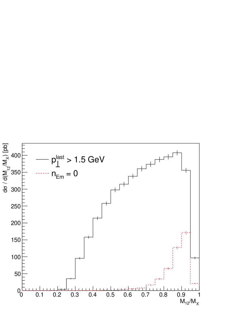
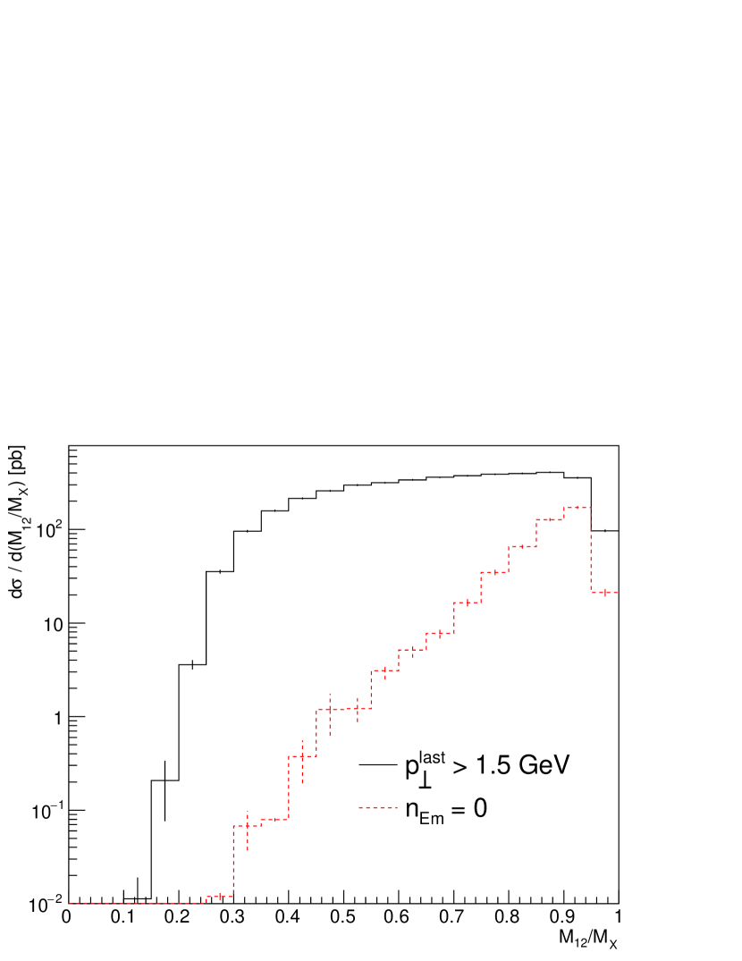
Figure 3: The differential exclusive di-jet cross section for $pp$ collisions at $\sqrt{s}=13\,\mbox{TeV}$ as a function of $M_{12}/M_{X}$. The phase space is defined by $p_{\perp}^{\mathrm{jet}1,2}>40\,\mbox{GeV}$, $|\eta^{\mathrm{jet}1,2}|<2.5$ and $\xi_{1,2}<0.03$. The blue curve represents the cross section with the final-state shower only in contrast to the black curve where the initial-state shower is included as well (down to $1.5\,\mbox{GeV}$). Cross sections with no initial-state radiation correspond to the classical implementation of the Durham formalism.

The exclusive cross section is less sensitive to the space-like emissions if only the events with, for example $M_{12}/M_{X}>0.8$ are accepted as is demonstrated in figure 4.

Here, the left plot shows that the di-jet cross section consists of events either with $p_{\perp}^{\mathrm{last}}\sim 40\,\mbox{GeV}$ where there was typically no space-like emission and $p_{\perp}^{\mathrm{last}}$ was identified with the hard scale of the process, or events with $p^{\mathrm{last}}_{\perp}\sim 3\,\mbox{GeV}$. In this case, there are usually many emissions and $p_{\perp}^{\mathrm{last}}$ denotes the transverse momentum of the latest one with the smallest $p_{\perp}$.

It can be seen the di-jet cross section differential in the $p_{\perp}$ of the last ISR emission peaks for $p^{\mathrm{last}}_{\perp}\sim 3\,\mbox{GeV}$ and decreases for lower transverse momenta.

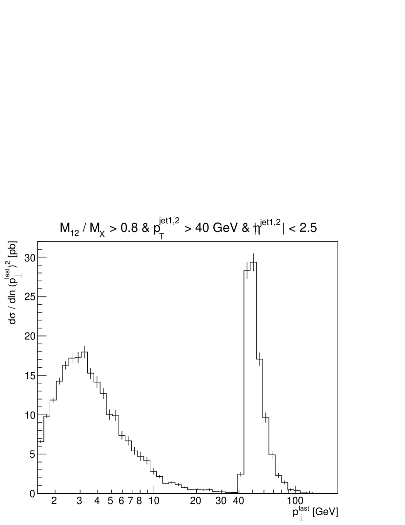
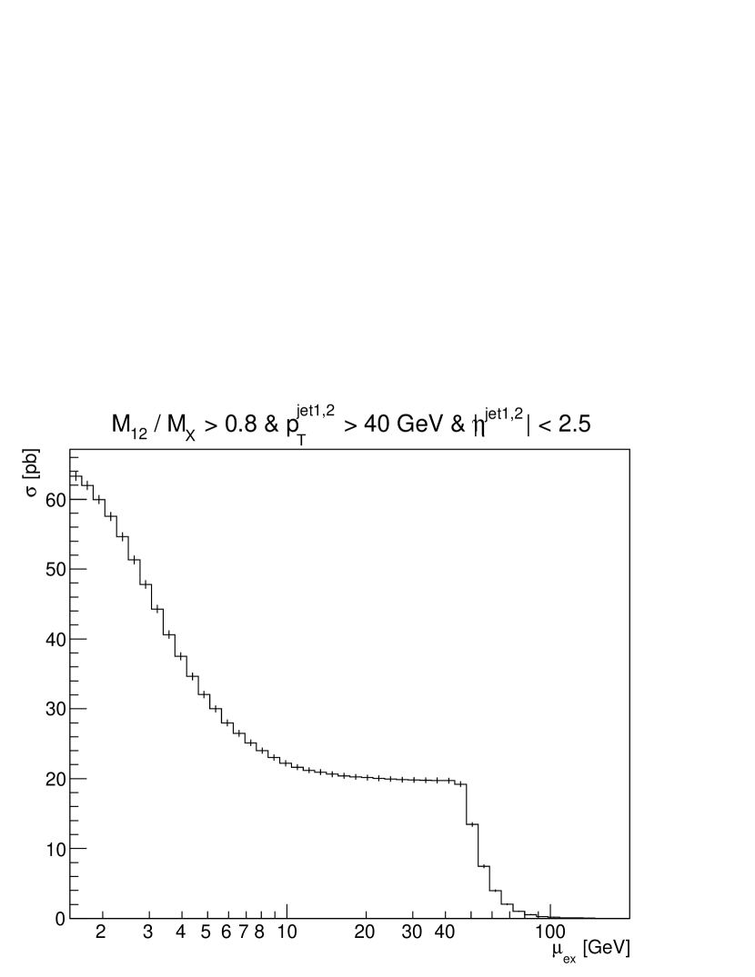
Figure 4: The exclusive di-jet cross section for $pp$ collisions at $\sqrt{s}=13\,\mbox{TeV}$ differential in $\ln(p_{\perp}^{\mathrm{last}})^{2}$ (left). The variable $p_{\perp}^{\mathrm{last}}$ denotes the scale of the “softest” ISR emission. For events absent from any ISR emissions $p_{\perp}^{\mathrm{last}}$ is identified with the scale of the sub-process. The total exclusive cross section as a function of the cut-off scale $\mu_{exc}$ is shown on the right. This scale means that that only events with $p_{\perp}^{\mathrm{last}}>\mu_{exc}$ are accepted. As is seen from the right plot the incorporation of the ISR with $\mu_{exc}=1.5\,\mbox{GeV}$ increases the CEP cross section from $19\,\text{pb}$ to $63\,\text{pb}$. The phase space is defined by $p_{\perp}^{\mathrm{jet}1,2}>40\,\mbox{GeV}$, $|\eta^{\mathrm{jet}1,2}|<2.5$, $M_{12}/M_{X}>0.8$ and $\xi_{1,2}<0.03$.

More comprehensive picture of the situation provides the two-dimensional plot (Fig. 5), where the correlation of the mass ratio and the $p_{\perp}^{\mathrm{last}}$ for a particular event is shown. The depletion of the emissions for $p_{\perp}^{\mathrm{last}}$ slightly below $40\,\mbox{GeV}$ is partially due to the small $gg\to ggg$ colour singlet cross section and partially just a statistical effects given by the low probability of having no further emission below such high $p_{\perp}$. The tree-level $gg\to ggg$ spin-singlet colour-singlet cross section in the analytic form is provided in Harland-Lang:2015faa . This cross section is zero in the “parton-shower” limit where one of the outgoing gluons has small $p_{T}$ compared to the remaining two and $\hat{t}=\hat{u}=-\hat{s}/2$, where the Mandelstam variables are derived from the two hardest gluons whereas the softest one is supposed to be part of the shower. Such behaviour agrees with our calculations based on procedure introduced in section 4.

The cut-off parameter $\mu_{exc}$ can be understood as a variable which describes the transition between perturbative and non-perturbative region. Not only due to the possible overlap with the double Pomeron exchange process but also because the scale $\mu_{exc}$ denotes the minimal allowed $p_{\perp}$ of the ISR emission and the $p_{\perp}$ of the softest emission is simultaneously the highest allowed transverse momentum of the screening gluon. Choosing small $\mu_{exc}$ leads to low $p_{\perp}^{\mathrm{last}}$ and consequently the main contribution to the exclusive luminosity given by integral (3.1) stems from small transverse momenta, i.e. smaller than $1$ GeV, where the perturbative QCD is not justified Khoze:2004yb .

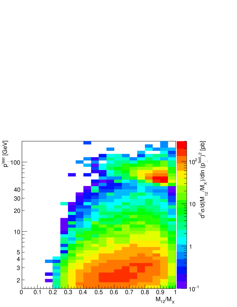
Figure 5: The exclusive di-jet cross section for $pp$ collisions at $\sqrt{s}=13\,\mbox{TeV}$ double differential in $M_{12}/M_{X}$ and $\ln\,(p_{\perp}^{\mathrm{last}})^{2}$. For sake of clarity the vertical axis is denominated directly in $p_{\perp}^{\mathrm{last}}$. The phase space is defined by $p_{\perp}^{\mathrm{jet}1,2}>40\,\mbox{GeV}$, $|\eta^{\mathrm{jet}1,2}|<2.5$ and $\xi_{1,2}<0.03$.

Finally in table 1 we show the contribution to the exclusive cross section from the different possible hard sub-process.

Table 1: The table demonstrates how the particular hard sub-processes in P

YTHIA

8 contribute to the total exclusive cross section of the di-jet production at LHC ($\sqrt{s}=13\,\mbox{TeV}$). The hard processes are defined using the Pythia convention and are accompanied by the Pythia process Id PythiaQCD . The letter $q$ denotes any light quark flavour, therefore, e.g. $gg\to q\bar{q}$ represents the sum of $gg\to u\bar{u}$, $gg\to d\bar{d}$ and $gg\to s\bar{s}$ cross sections. The jets in the di-jet system are required to have $p_{\perp}^{\mathrm{jet}1,2}>40\,\mbox{GeV}$ and $|\eta^{\mathrm{jet}1,2}|<2.5$. In addition the leading protons momentum loss $\xi$ must be $\xi_{1,2}<0.03$. The $\sigma^{n_{Em}=0}_{exc}$ are the exclusive cross sections with no initial-state radiation. The $\sigma_{exc}$ and $\sigma^{M_{12}/M_{X}>0.8}_{exc}$ are the exclusive cross section with allowed initial-state radiation down to $1.5\,\mbox{GeV}$; the last one has an additional constrain $M_{12}/M_{X}>0.8$.

Id	Process	$\sigma^{n_{Em}=0}_{exc}\;[\text{pb}]$	$\sigma_{exc}\;[\text{pb}]$	$\sigma^{M_{12}/M_{X}>0.8}_{exc}\;[\text{pb}]$
$111$	$gg\to gg$	$23$	$173$	$57$
$112$	$gg\to q\bar{q}$	$10.6\times 10^{-3}$	$0.6$	$56\times 10^{-3}$
$113$	$qg\to qg$	$-$	$30$	$5.8$
$114$	$qq^{\prime}\to qq^{\prime}$	$-$	$1.3$	$94\times 10^{-3}$
$115$	$q\bar{q}\to gg$	$-$	$10.5\times 10^{-3}$	$83\times 10^{-6}$
$116$	$q\bar{q}\to q^{\prime}\bar{q}^{\prime}$	$-$	$16\times 10^{-3}$	$0.5\times 10^{-3}$
$121$	$gg\to c^{\prime}\bar{c}^{\prime}$	$4.8\times 10^{-3}$	$0.2$	$21\times 10^{-3}$
$122$	$q\bar{q}\to c^{\prime}\bar{c}^{\prime}$	$-$	$4.5\times 10^{-3}$	$57\times 10^{-6}$
$123$	$gg\to b^{\prime}\bar{b}^{\prime}$	$20\times 10^{-3}$	$0.3$	$51\times 10^{-3}$
$124$	$q\bar{q}\to b^{\prime}\bar{b}^{\prime}$	$-$	$4.4\times 10^{-3}$	$53\times 10^{-6}$
	all	23	205	63

One can see that even with space-like parton showers enabled, the $gg\to gg$ sub-process dominates. The second largest cross section is given by the $qg\to qg$ process which is forbidden without ISR. Consequently, the fraction of di-jet events where at least one of them is quark-induced with respect to the total exclusive di-jet cross section is much higher than $\sim\!10^{-4}$ predicted in Harland-Lang:2014lxa . This fact makes it problematic to use the CEP as a pure source of gluonic jets.

Within the collinear approximation the $gg\to q\bar{q}$ cross section is predicted to be suppressed as $m_{q}^{2}/s$ with respect to the $gg\to gg$ cross section. This is well-known consequence of the spin singlet selection rule. It is interesting that without using such collinear approximation the exclusive production of light flavour $q\bar{q}$ jets is not so heavily suppressed since the $|J_{z}|=2$ contribution, absent in collinear case, has a similar size and is quark-mass independent Harland-Lang:2014lxa . This effect is even stronger if the ISR is included.

Nevertheless, for higher $M_{12}/M_{X}$ the fraction of the heavy flavours jets with respect to the whole CEP’s di-jet sample is still predicted to be lower compared to the DPE which makes such quantity a vital experimental variable for studying the transition region between CEP and DPE as was first done at the Tevatron Aaltonen:2007hs .

In figure 6 we have tried to compare the results from our CEP program for the distribution in $M_{12}/M_{X}$ with data published by the CDF collaboration Aaltonen:2007hs . The comparison is a bit uncertain as the data has not been corrected to the hadron-level, and the acceptance in different regions of phase space is difficult to disentangle. Nevertheless we have checked that our implementation of the DPE gives results similar to what was published in Aaltonen:2007hs for normalised distributions.

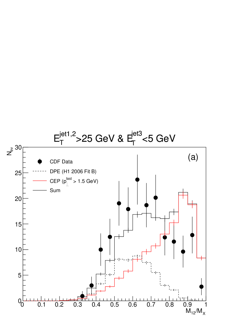
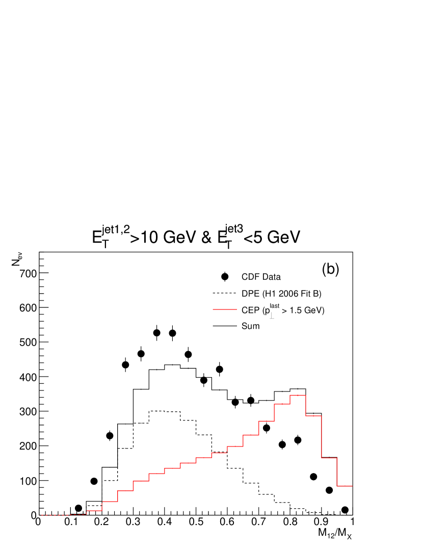
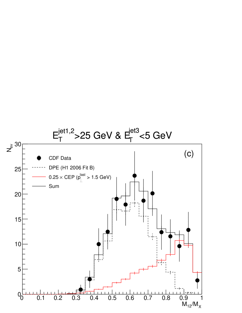
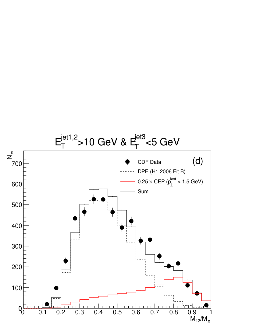
Figure 6: The di-jet event counts binned in $M_{12}/M_{X}$ variable as measured by the CDF collaboration Aaltonen:2007hs in $p\bar{p}$ collisions at energy $\sqrt{s}=1.96\,\mbox{TeV}$. These measured event counts (not corrected for the detector related effects) are compared with the DPE contribution (black dashed line) and CEP contribution (red line) and their sum (black solid line). The normalization of these curves is fixed in such a way that the total predicted event count is the same as in data. In figures c and d the CEP contributions were scaled down by a factor of $0.25$ compared to their nominal value.

Our DPE implementation uses diffractive parton densities, as measured e.g. by HERA. Specifically, we will here use the HERA H1 2006 Fit B DPDFs Aktas:2006hy with, for simplicity, the same soft survival probability as for the CEP process, although we are aware that the soft survival probability may very well be different for the DPE process as compared to the CEP one. Technically the DPE simulation is done in Pythia (with the same setting as for the CEP) by colliding two hadrons, the Pomerons, with energies $\frac{1}{2}\xi_{1}\sqrt{s}$ and $\frac{1}{2}\xi_{2}\sqrt{s}$ and with parton densities described by the HERA DPDFs.

In figure 6a and b we show the results of simply adding our CEP generated events for two different selection cuts (two jets above $10$ and $25$ GeV respectively and no third jet above $5$ GeV). Further selection criteria, identical for both phase spaces are given in Aaltonen:2007hs . We see that the addition of CEP severely overshoots the data in the exclusive region of high $M_{12}/M_{X}$. There are, however, many uncertainties, especially when it comes to the soft survival probability, both for the CEP and DPE contribution. As a demonstration we show in figure 6c and d the effect of introducing a relative normalization factor of $0.25$ between the CEP and DPE contribution, which gives a quite reasonable description of the data. We note that our CEP, as expected, contributes quite noticeably also away from the purely exclusive region. A more detailed study of the differences between our new CEP procedure and the DPE one, especially in the regions of the Pomeron remnants in DPE, may result in observables that could further improve the experimental separation between the two processes.

5.2 Higgs production

The possibility to measure the Higgs boson in the central exclusive production was studied extensively in the last decade Cox:2005if ; Heinemeyer:2007tu . The discussion was mainly focused on the dominant decay channel $gg\to H\to b\bar{b}$ with a standard model branching ratio of $59\%$.

The main advantage of this production mechanism is a huge suppression of the irreducible standard model background from $gg\to b\bar{b}$ due to the $J_{z}=0$ selection rule in CEP. Furthermore, the scalar nature of the Higgs boson means that the ratio of exclusive to inclusive cross sections is relatively enhanced as compared to the background, as the spin and colours have to match also in the inclusive sub-process. Both these effects improve the signal/background ratio for the Higgs boson production compared to the inclusive production.

The main background to the exclusive Higgs boson production comes from the $gg\to gg$ sub-process, which can be substantially suppressed using b-jet tagging techniques. The other experimental challenge is the detection of the scattered protons in the forward detectors in a high pile-up environment where protons from several interactions can simultaneously hit the forward detector within one bunch crossing.

Note, that the cross section of the Higgs boson production in CEP is only around $2\,\text{fb}$, including the calculated soft survival probability of $0.06$, which is about four order lower than the inclusive Higgs cross section $\sim 20\,\text{pb}$. The signal event’s count is further reduced due to selection criteria and inefficiency of the b-jet tagging. In particular, the QCD background must be suppressed by selecting only high $p_{\perp}$ b-jets (comparable to $M_{H}/2$) because the Higgs boson decay is isotropic whereas the QCD jet production is suppressed at high $p_{\perp}$ at least as $1./p_{\perp}^{4}$.

We included the Higgs boson production in the process library of our program to study the production rates compared to the background processes. The simulation incorporates the parton showers as well as hadronisation of the resulting partons into “stable” particles, where the particles with lifetime higher than $0.01\,\text{mm/c}$ are considered to be stable. The inclusion of initial-state showers have negligible effect on the exclusive Higgs cross section but can substantially increase the $gg\to b\bar{b}$ background and spoil the signal significance (see table 1).

We have simulated Higgs production at the LHC at $\sqrt{s}=13$ TeV. The hard scale is set to be equal to the Higgs mass for the signal, and to $p_{\perp}$ of the leading jet for the background, the cut-off for the space-like showers is 1.5 GeV in both cases. To pass the selection cuts, the events are required to contain at least two b-jets with $p_{\perp}$ higher than 50 GeV and, additionally, the ratio $M_{12}/M_{X}$ must be higher than 0.9. As before, the jets are identified using anti-$k_{\perp}$ jet algorithm with $R=0.7$ and a jet is tagged as a b-jet if it contains at least one bottom hadron. For now, the kinematics of the scattered protons is not constrained. The result of these calculations is presented in figure 7, where the dotted lines indicate the fraction of the cross section without space-like emissions. It is obvious that events with space-like emissions play a role only for the $gg\to b\bar{b}$ process and their rate can be probably further reduced using more sophisticated selection techniques. Note that the signal peak is a little bit shifted towards lower values compared to the Higgs mass $m_{H}=125$ GeV, due to the fact that sometimes not all produced particles in the hadronisation of the b-quarks are incorporated into the b-jets.

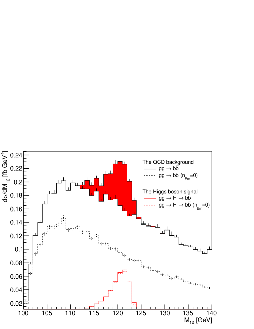
Figure 7: The differential distribution of the invariant mass of two leading b-jets for $pp$ CEP at LHC ($\sqrt{s}=13\,\mbox{TeV}$). To enhance the signal fraction the additional cuts $p^{\mathrm{jet}1,2}_{T}>50\,\mbox{GeV}$ and $M_{12}/M_{X}>0.9$ were applied. The differential cross section stemming from the Higgs decay is given by the red solid curve and the QCD background from $gg\to b\bar{b}$ process is given by the black curve. In addition, the dashed curves indicate the corresponding cross section if initial-state showers are not considered.

In reality, the forward proton spectrometers installed to ATLAS and CMS have a limited acceptance in $\xi$, the lowest measurable value of $\xi$ is projected to be around $0.015$ which restricts the minimal value of the exclusive system mass to $M_{X}=\xi\sqrt{s}=195\,\mbox{GeV}$. This acceptance limit makes the observation of single Higgs boson production without no other activity impossible. On the other hand, there is still a hope of the signal of the Higgs boson accompanied by jets originating from the space-like emissions. To see the size of such cross section we plot the b-jets cross section (both of them must still have $p_{\perp}>50\,\mbox{GeV}$) in the mass window between $116$ and $127\,\mbox{GeV}$ where the signal peak is expected. This cross section is shown in figure 8 as a function of the $M_{12}/M_{X}$ ratio both for signal and background Monte Carlo sample. The ratio of these cross sections roughly matches the signal/background estimate. It is quite good for $M_{12}/M_{X}>0.9$ which is the kinematic phase space shown in figure 7 whereas deteriorates for lower values of $M_{12}/M_{X}$.

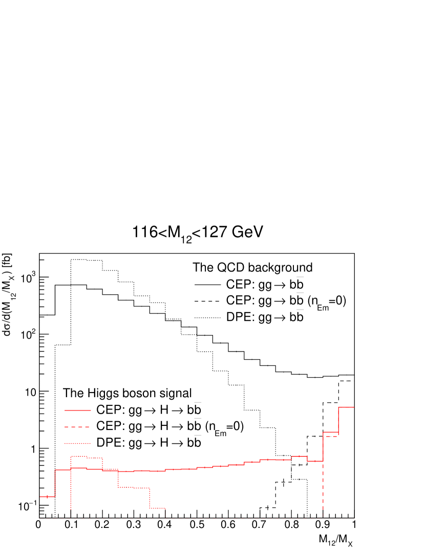
Figure 8: The cross section for the CEP production of two b-jets at LHC with $p_{\perp}^{\mathrm{jet}1,2}>50$ GeV and invariant mass $116<M_{12}<127$ GeV differential in $M_{12}/M_{X}$. The red and black solid lines denote the cross section rising from the Higgs boson decay and the QCD background, respectively. The dashed lines denoted the corresponding cross sections with no initial-state radiation. In addition, the double Pomeron cross sections for Higgs production and the QCD $gg\to b\bar{b}$ process are plotted by the dotted lines.

To reach the acceptance of LHC forward detectors, the mass ratio must be lower than 0.6. Assuming $0.5<M_{12}/M_{X}<0.6$ the signal cross section of the b-jets production is around 0.05 fb and is around 200 times smaller than the QCD background. This small signal cross section and huge background contamination leads to a luminosity of $\sim\!60,000\,\text{fb}^{-1}$ to reach $4$-sigma precision. Although the possibility of measure the Higgs production in this experimental setup is rather academic, our framework allows to determine such cross sections as well as more realistically evaluate the contamination from the QCD background processes.

In figure 8 we also show the corresponding calculation from the DPE process, which becomes significant at low values of $M_{12}/M_{X}$ both for the signal and background, but clearly does not give any increase in the significance.

5.3 $Z^{0}$ production

Considering the acceptance of the forward proton spectrometers of the ATLAS and CMS detectors, which is around $0.015<\xi<0.1$, the mass of $Z^{0}$ resonance is much smaller than the acceptance limit $M_{X}\!\approx\!200\,\mbox{GeV}$. This makes the study of direct production of the $Z^{0}$ within the CEP mechanism even more impossible than the Higgs. Moreover, the $Z^{0}$ is produced by $q\bar{q}\to Z^{0}$ sub-process, which cannot be handled directly in the standard implementations of the Durham model.

However, our model allows for initial-state radiation from the partons entering to the hard sub-process, which can change the identity of incoming quarks to gluons, which can be then treated using the standard Durham exclusive luminosity. To do so, at least one $g\to q\bar{q}$ emission from each side is needed.

Due to the colour singlet nature of the $Z^{0}$ and the fusing quarks, there will probably be a non-negligible cross section for no space like emissions and $q\bar{q}$ CEP luminosity with a screening quark as discussed briefly above. Here, we will make no attempt to evaluate such cross section although our model can, in principle, be extended to cover this production mechanism as well.

The other mechanism for central (semi-)exclusive production of a $Z^{0}$ is through DPE. To estimate such a cross section we use the procedure described in section 5.1, where we again we assume that the DPE soft survival probability is the same as in CEP. Contrary to the CEP where the $M_{X}$ mass is higher than $M_{Z}$ mostly due to space like emissions, in DPE both the space like emissions and the Pomeron remnants contribute to the mass.

We will look at semi-exclusive $Z^{0}\to\mu^{-}\mu^{+}$ production at the LHC at $\sqrt{s}=13$ TeV, requiring a minimum transverse momentum of $30$ GeV for the muons in the pseudorapidity region of $|\eta|<2.5$. Both quasi-elastically scattered protons are required to have $0.015<\xi_{1,2}<0.1$ in accordance to the acceptance of forward proton spectrometers. The electroweak process $q\bar{q}\to\mu\bar{\mu}$ includes both $Z^{0}$ exchange and $\gamma$ exchange as well as the interference terms. We find that the resulting DPE cross section is about ten times higher than for CEP. Quantitatively the CEP cross section is around $3.5$ fb compared to $40$ fb for DPE. The $Z^{0}$ can be produced also via the exclusive photoproduction. The predicted cross section for this process, including $Z^{0}\to\mu^{-}\mu^{+}$ branching ratio, is, however, about $0.3$ fb Motyka:2008ac and would be even smaller if the selection criteria for muons $p_{T}$ and pseudorapidity had been applied.

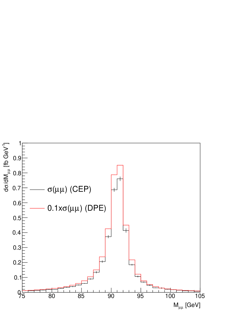
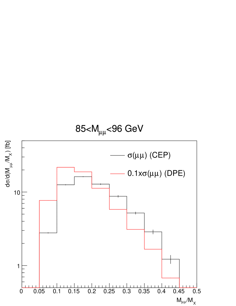
Figure 9: The differential cross section of $pp\to p+\mu^{-}\mu^{+}X^{\prime}+p$ process as a function of the invariant mass of the $\mu^{-}\mu^{+}$ pair (left plot) and of the ratio $M_{\mu\mu}/M_{X}$ (right plot). The black lines show the CEP contribution whereas the DPE result is given by the red lines. The DPE cross sections are normalised by a factor of $0.1$. In the CEP calculations the $\mu_{exc}$ cut-off parameter is set to 1.5 GeV.

The shapes of the $M_{\mu\mu}$ and $M_{\mu\mu}/M_{X}$ distributions are compared in figure 9. The shapes of $M_{\mu\mu}/M_{X}$ are rather similar for both processes, with the DPE curve somewhat shifted towards lower values as compared to the CEP one which prefers more “exclusive” configurations.

6 Conclusions

In this paper we introduced a new Monte Carlo implementation of the Durham formalism to calculate the central exclusive processes in $pp$ and $p\bar{p}$ collisions. Our model is based on P YTHIA 8 generator, and naturally incorporates partonic showers and hadronisation, as well as multi-parton interactions.

The main advantage of our implementation is the possibility to study the effects of initial-state parton radiation on CEPs. This is done by allowing that any inclusively produced sub-process is converted to an exclusive at any stage in the shower. To do this we have implemented a colour and spin decomposition of the initial-state shower in P YTHIA 8 which, together with a similarly decomposed (user supplied) matrix element, can be used to determine the probability that a given partonic state can be exclusive.

We have shown that this way of approximating higher jet multiplicities gives rise to to new, non-trivial, physical consequences. In particular, for exclusive di-jet production, it leads to event topologies with medium values of $M_{12}/M_{X}$ which naturally fill the gap between double Pomeron exchange and pure central exclusive production. Moreover, the incorporation of the parton showers enables the generation of quark-initiated processes such as $Z^{0}$ production.

All predicted cross sections depend on the parameter $\mu_{exc}$, the scale related the transition between the perturbative and non-perturbative region in the parton shower. The actual value of $\mu_{exc}$ will have to be determined from experiment. For the time being we set its value equal to $1.5\,\mbox{GeV}$.

The cross sections also depend on the soft survival probability used. Here we have used the MPI model in P YTHIA 8 to simply estimate the probability of having no additional scatterings, equating this to the soft survival probability. Although this procedure was suggested long ago, it has not been properly investigated, and we intend to return with a detailed study of this model in a future publication.

Currently, the program process library includes QCD $2\to 2$ processes, $H$ production, $Z^{0}$ production and $\gamma\gamma$ production, but it can be easily extended. In particular, it would be interesting to add production of vector mesons ($\rho$, $\phi$, …) and/or quarkonia $\chi_{c,b}$. These processes have large cross sections which make them experimentally accessible even at low luminosities.

Our framework to treat colour and spin states within the partonic shower is rather general and can, in principle, be extended to simulate the central exclusive processes initiated by $q\bar{q}$ fusion, in addition to standard $gg$-initiated processes. Here a screening quark rather than screening gluon is exchanged to cancel the colour flow. Such processes would be especially interesting for e.g. central exclusive $Z^{0}$ production.

It should also be possible to extend our treatment of the colour and spin structure of the parton showers to treat final-state splittings. This would give an additional way of studying approximate higher order effects in the hard sub-process matrix elements.

These and other possible improvements will be discussed in a future publication.

Appendix A Colour emission tensors

In this section the list of all linear transformations which relate the colour emission tensor before and after the emission is given. New coefficients are labelled by the prime symbol. If the expression for any coefficient of the colour emission tensor is missing, this coefficient is zero.

Adding of gluon:

• $g\to(g\to g)$:

  $$A^{\prime}_{12} = -\frac{1}{2}B_{432}-\frac{1}{2}B_{234}$$

  $$A^{\prime}_{13} = +\frac{1}{2}B_{423}+\frac{1}{2}B_{342}+\frac{1}{2}B_{324}+\frac{1}{2}B_{243}+3A_{13}$$

  $$A^{\prime}_{14} = -\frac{1}{2}B_{432}-\frac{1}{2}B_{234}$$

  $$B^{\prime}_{234} = -\frac{1}{2}A_{14}-\frac{1}{2}A_{12}$$

  $$B^{\prime}_{243} = +\frac{3}{2}B_{243}+\frac{1}{2}A_{12}$$

  $$B^{\prime}_{324} = +\frac{3}{2}B_{324}+\frac{1}{2}A_{14}$$

  $$B^{\prime}_{342} = +\frac{3}{2}B_{342}+\frac{1}{2}A_{12}$$

  $$B^{\prime}_{423} = +\frac{3}{2}B_{423}+\frac{1}{2}A_{14}$$

  $$B^{\prime}_{432} = -\frac{1}{2}A_{14}-\frac{1}{2}A_{12}$$

• $g\to(q\to q)\;\;\text{or}\;\;g\to(q\to\bar{q})$:

  $$D^{\prime}_{ij} = K_{1}$$

  $$C^{\prime}_{1} = K_{3}$$

  $$C^{\prime}_{1c} = K_{2}$$

• $g\to(\bar{q}\to q)\;\;\text{or}\;\;g\to(\bar{q}\to\bar{q})$:

  $$D^{\prime}_{ij} = K_{1}$$

  $$C^{\prime}_{1c} = K_{3}$$

  $$C^{\prime}_{2} = K_{2}$$

• $g\to(g\to q)\;\;\text{or}\;\;g\to(g\to\bar{q})$:

  $$D_{ij} = \frac{1}{2}C_{2c}+\frac{1}{2}C_{1c}+\frac{1}{2}C_{2}+\frac{1}{2}C_{1}+3D_{ij}$$

  $$C_{1} = \frac{3}{2}C_{1}$$

  $$C_{1c} = \frac{3}{2}C_{1c}$$

  $$C_{2} = \frac{3}{2}C_{2}$$

  $$C_{2c} = \frac{3}{2}C_{2c}$$

• $g\to(q\to g)$:

  $$A^{\prime}_{13} = D_{ij}$$

  $$B^{\prime}_{243} = C_{2c}$$

  $$B^{\prime}_{324} = C_{1c}$$

• $g\to(\bar{q}\to g)$:

  $$A^{\prime}_{13} = D_{ij}$$

  $$B^{\prime}_{423} = C_{2}$$

  $$B^{\prime}_{342} = C_{1}$$

Adding of quark:

• $q\to(q\to q)\;\;\text{or}\;\;q\to(q\to\bar{q})$:

  $$K^{\prime}_{1} = \frac{1}{2}K_{3}+\frac{1}{2}K_{2}+\frac{4}{3}K_{1}$$

  $$K^{\prime}_{3} = -\frac{1}{6}K_{3}$$

  $$K^{\prime}_{2} = -\frac{1}{6}K_{2}$$

• $q\to(q\to g)$:

  $$D^{\prime}_{ij} = \frac{1}{2}C_{2c}+\frac{1}{2}C_{1c}+\frac{4}{3}D_{ij}$$

  $$C^{\prime}_{1c} = -\frac{1}{6}C_{1c}$$

  $$C^{\prime}_{2c} = -\frac{1}{6}C_{2c}$$

• $q\to(g\to q)\;\;\text{or}\;\;q\to(g\to\bar{q})$:

  $$K^{\prime}_{1} = \frac{5}{18}C_{2c}+\frac{1}{36}C_{1c}+\frac{5}{18}C_{2}+\frac{1}{36}C_{1}+\frac{2}{3}D_{ij}$$

  $$K^{\prime}_{3} = -\frac{1}{6}C_{2}+\frac{7}{12}C_{1}$$

  $$K^{\prime}_{2} = -\frac{1}{6}C_{2c}+\frac{7}{12}C_{1c}$$

• $q\to(g\to g)$:

  $$D^{\prime}_{ij} = +\frac{1}{36}B_{432}+\frac{5}{18}B_{423}+\frac{5}{18}B_{342}+$$

  $$+\frac{1}{36}B_{324}+\frac{1}{36}B_{243}+\frac{1}{36}B_{234}+\frac{2}{3}A_{13}$$

  $$C^{\prime}_{1c} = -\frac{1}{12}B_{432}-\frac{1}{6}B_{342}+\frac{7}{12}B_{324}-$$

  $$-\frac{1}{12}B_{234}+\frac{1}{4}A_{14}$$

  $$C^{\prime}_{2c} = -\frac{1}{12}B_{432}-\frac{1}{6}B_{423}+\frac{7}{12}B_{243}-$$

  $$-\frac{1}{12}B_{234}+\frac{1}{4}A_{12}$$

Adding of anti-quark:

• $\bar{q}\to(\bar{q}\to q)\;\;\text{or}\;\;\bar{q}\to(\bar{q}\to\bar{q})$:

  $$K^{\prime}_{1} = \frac{1}{2}K_{3}+\frac{1}{2}K_{2}+\frac{4}{3}K_{1}$$

  $$K^{\prime}_{3} = -\frac{1}{6}K_{3}$$

  $$K^{\prime}_{2} = -\frac{1}{6}K_{2}$$

• $\bar{q}\to(\bar{q}\to g)$:

  $$D^{\prime}_{ij} = \frac{1}{2}C_{2}+\frac{1}{2}C_{1}+\frac{4}{3}D_{ij}$$

  $$C^{\prime}_{1} = -\frac{1}{6}C_{1}$$

  $$C^{\prime}_{2} = -\frac{1}{6}C_{2}$$

• $\bar{q}\to(g\to q)\;\;\text{or}\;\;\bar{q}\to(g\to\bar{q})$:

  $$K^{\prime}_{1} = +\frac{1}{36}C_{2c}+\frac{5}{18}C_{1c}+\frac{1}{36}C_{2}+\frac{5}{18}C_{1}+\frac{2}{3}D_{ij}$$

  $$K^{\prime}_{3} = -\frac{7}{12}C_{2c}-\frac{1}{6}C_{1c}$$

  $$K^{\prime}_{2} = -\frac{7}{12}C_{2}-\frac{1}{6}C_{1}$$

• $\bar{q}\to(g\to g)$:

  $$D^{\prime}_{ij} = +\frac{1}{36}B_{432}+\frac{1}{36}B_{423}+\frac{1}{36}B_{342}+$$

  $$+\frac{5}{18}B_{324}+\frac{5}{18}B_{243}+\frac{1}{36}B_{234}+\frac{2}{3}A_{13}$$

  $$C^{\prime}_{1} = -\frac{1}{12}B_{432}+\frac{7}{12}B_{342}-\frac{1}{6}B_{324}-$$

  $$-\frac{1}{12}B_{234}+\frac{1}{4}A_{12}$$

  $$C^{\prime}_{2} = -\frac{1}{12}B_{432}+\frac{7}{12}B_{423}-\frac{1}{6}B_{243}-$$

  $$-\frac{1}{12}B_{234}+\frac{1}{4}A_{14}$$

Appendix B Spin emission tensors

In this section the spin emission matrices are provided for all possible kinds of splittings. In reality approximate the higher order matrix element squared, these splitting matrices should incorporate an additional normalisation factor $(4\pi)^{2}\frac{\alpha_{s}}{2\pi}\frac{1-z}{z}\frac{1}{p_{\perp}^{2}}$. Since only the ratio $\frac{\sigma^{\prime s}}{\sigma^{\prime i}}$ is relevant in our framework and the normalisation factors would be the same in numerator and denominator; these factors can be simply omitted as they cancel in the ratio.

Note that the spin averaged splittings $P_{\mathrm{avg}}$ used in relation (49) can be obtained (up to the normalisation arising from the colour part) as a sum of the “corner” elements of the spin emission matrix:

$$P_{\mathrm{avg}}(z)\sim P^{1em}_{11}+P^{1em}_{14}+P^{1em}_{41}+P^{1em}_{44}$$

The spin emission matrices are the following:

$$P^{1em}_{g\to g}=\leavevmode\resizebox{200.0003pt}{}{$\left(\begin{matrix}\frac{1}{z}+\frac{2}{1-z}-1-z-z^{2}&-z(1-z)\,\mathrm{e}^{+2i\phi}&-z(1-z)\,\mathrm{e}^{-2i\phi}&\frac{1}{z}-3+3z-z^{2}\\ -\frac{1-z}{z}\,\mathrm{e}^{-2i\phi}&\frac{2z}{1-z}&0&-\frac{1-z}{z}\,\mathrm{e}^{-2i\phi}\\ -\frac{1-z}{z}\,\mathrm{e}^{+2i\phi}&0&\frac{2z}{1-z}&-\frac{1-z}{z}\,\mathrm{e}^{+2i\phi}\\ \frac{1}{z}-3+3z-z^{2}&-z(1-z)\,\mathrm{e}^{+2i\phi}&-z(1-z)\,\mathrm{e}^{-2i\phi}&\frac{1}{z}+\frac{2}{1-z}-1-z-z^{2}\end{matrix}\right)$}$$

$$P^{1em}_{g\to q}=\leavevmode\resizebox{180.00027pt}{}{$\left(\begin{matrix}z^{2}&-z(1-z)\mathrm{e}^{+2i\phi}&-z(1-z)\mathrm{e}^{-2i\phi}&(1-z)^{2}\\ 0&0&0&0\\ 0&0&0&0\\ (1-z)^{2}&-z(1-z)\mathrm{e}^{+2i\phi}&-z(1-z)\mathrm{e}^{-2i\phi}&z^{2}\end{matrix}\right)$}$$

$$P^{1em}_{q\to g}=\left(\begin{matrix}\frac{1}{z}&0&0&\frac{(1-z)^{2}}{z}\\ -\frac{1-z}{z}\mathrm{e}^{-2i\phi}&0&0&-\frac{1-z}{z}\mathrm{e}^{-2i\phi}\\ -\frac{1-z}{z}\mathrm{e}^{+2i\phi}&0&0&-\frac{1-z}{z}\mathrm{e}^{+2i\phi}\\ \frac{(1-z)^{2}}{z}&0&0&\frac{1}{z}\end{matrix}\right)$$

$$P^{1em}_{q\to q}=\left(\begin{matrix}\frac{1+z^{2}}{1-z}&0&0&0\\ 0&\frac{2z}{1-z}&0&0\\ 0&0&\frac{2z}{1-z}&0\\ 0&0&0&\frac{1+z^{2}}{1-z}\end{matrix}\right)$$

Appendix C Example of the sub-process definition

In this section an example of the sub-process definition is presented for $q\bar{q}\to gg$ process. The amplitude of this process, written in the colour basis, has the following form:

$$A^{\lambda}_{a_{l1}a_{r1}\to x_{3}x_{4}}=A^{\lambda}_{1}\,(T^{x_{3}}T^{x_{4}})_{a_{r1}a_{l1}}+A^{\lambda}_{2}\,(T^{x_{4}}T^{x_{3}})_{a_{r1}a_{l1}},$$

where $\lambda$ denotes helicity state of both incoming and outgoing particles. The indexes $a_{l1}$, $a_{r1}$ and $x_{3}$, $x_{4}$ denote the colour of incoming and outgoing particles and $T^{x_{3,4}}$ are the Gell-Mann matrices.

Within our framework, the colour matrix $M^{ij}$ of the process must be provide by means of three colour basis vectors:

$$\mathcal{B}_{ll^{\prime}} = \delta_{a_{l1}a^{\prime}_{l1}}\delta_{a_{r1}a^{\prime}_{r1}}\qquad\qquad\mathcal{B}_{lr}=\delta_{a_{l1}a_{r1}}\delta_{a^{\prime}_{l1}a^{\prime}_{r1}}$$

$$\mathcal{B}_{lr^{\prime}} = \delta_{a_{l1}a^{\prime}_{r1}}\delta_{a^{\prime}_{l1}a_{r1}}$$

The colour matrix has the following form:

$$M^{11} = \;\frac{7}{12}\mathcal{B}_{ll^{\prime}}+\frac{1}{36}\mathcal{B}_{lr}\quad\,M^{12}=-\frac{1}{6}\mathcal{B}_{ll^{\prime}}+\frac{5}{18}\mathcal{B}_{lr}$$ (75)

$$M^{21} = -\frac{1}{6}\mathcal{B}_{ll^{\prime}}+\frac{5}{18}\mathcal{B}_{lr}\quad\,M^{22}=\frac{7}{12}\mathcal{B}_{ll^{\prime}}+\frac{1}{36}\mathcal{B}_{lr}$$

Therefore, for example, the $M^{11}_{\alpha}$ coefficients for this process are:

$$M^{11}_{ll^{\prime}}=\frac{7}{12}\qquad M^{11}_{lr}=\frac{1}{36}\qquad M^{11}_{lr^{\prime}}=0.$$ (76)

In addition to the colour matrix, the amplitudes for every helicity configuration must be given as well. These amplitudes are:

$$A_{1}^{+-\to+-} = +\frac{1}{\sqrt{2}}\,2g^{2}\frac{1}{s}\sqrt{tu}\,\mathrm{e}^{i\phi}$$ (77)

$$A_{2}^{+-\to+-} = -\frac{1}{\sqrt{2}}\,2g^{2}\frac{u}{s}\sqrt{\frac{u}{t}}\,\mathrm{e}^{i\phi}$$ (78)

$$A_{1}^{+-\to-+} = +\frac{1}{\sqrt{2}}\,2g^{2}\frac{t}{s}\sqrt{\frac{t}{u}}\,\mathrm{e}^{i\phi}$$ (79)

$$A_{2}^{+-\to-+} = -\frac{1}{\sqrt{2}}\,2g^{2}\frac{1}{s}\sqrt{tu}\,\mathrm{e}^{i\phi}$$ (80)

The $s$, $t$ and $u$ are the Mandelstam variables, $\phi$ is the azimuthal angle of first outgoing gluon and $g=\sqrt{4\pi\alpha_{s}}$. The amplitudes related by a parity transformation $-+\to-+$ and $-+\to+-$ can be obtained by the complex conjugation. The amplitudes of other helicity configurations are equal to zero. The normalisation factor $\frac{1}{\sqrt{2}}$ accounts for the identical particles in the final state. The fact that the outgoing particles are identical allows to derive the amplitudes (79-80) for the second helicity configuration $+-\to-+$ from the first one, eq. (77-78), by swapping the final state gluons ($t\leftrightarrow u$).

To summarise, each process in the process library is defined by the helicity amplitudes (77-80) and the corresponding colour matrix (75).

References

- (1) V.A. Khoze, A.D. Martin, M.G. Ryskin, Eur. Phys. J. C14, 525 (2000). DOI 10.1007/s100520000359
- (2) L.A. Harland-Lang, V.A. Khoze, M.G. Ryskin, W.J. Stirling, Int. J. Mod. Phys. A29, 1430031 (2014). DOI 10.1142/S0217751X14300312
- (3) J. Monk, A. Pilkington, Comput. Phys. Commun. 175, 232 (2006). DOI 10.1016/j.cpc.2006.04.005
- (4) M. Boonekamp, A. Dechambre, V. Juranek, O. Kepka, M. Rangel, C. Royon, R. Staszewski, (2011)
- (5) L.A. Harland-Lang, V.A. Khoze, M.G. Ryskin, Eur. Phys. J. C76(1), 9 (2016). DOI 10.1140/epjc/s10052-015-3832-8
- (6) T. Sjöstrand, S. Ask, J.R. Christiansen, R. Corke, N. Desai, P. Ilten, S. Mrenna, S. Prestel, C.O. Rasmussen, P.Z. Skands, Comput. Phys. Commun. 191, 159 (2015). DOI 10.1016/j.cpc.2015.01.024
- (7) B. Cox, J.R. Forshaw, L. Lonnblad, JHEP 10, 023 (1999). DOI 10.1088/1126-6708/1999/10/023
- (8) G. Ingelman, P.E. Schlein, Phys. Lett. B152, 256 (1985). DOI 10.1016/0370-2693(85)91181-5
- (9) L.A. Harland-Lang, V.A. Khoze, M.G. Ryskin, W.J. Stirling, Eur. Phys. J. C73, 2429 (2013). DOI 10.1140/epjc/s10052-013-2429-3
- (10) L.A. Harland-Lang, Phys. Rev. D88(3), 034029 (2013). DOI 10.1103/PhysRevD.88.034029
- (11) V.A. Khoze, A.D. Martin, M.G. Ryskin, Int. J. Mod. Phys. A30(08), 1542004 (2015). DOI 10.1142/S0217751X1542004X
- (12) V.A. Khoze, A.D. Martin, M.G. Ryskin, Eur. Phys. J. C24, 581 (2002). DOI 10.1007/s10052-002-0990-2
- (13) A.S. Kronrod, Soviet Physics Doklady 9, 17 (1964)
- (14) L.A. Harland-Lang, A.D. Martin, P. Motylinski, R.S. Thorne, Eur. Phys. J. C75(5), 204 (2015). DOI 10.1140/epjc/s10052-015-3397-6
- (15) M. Botje, Comput.Phys.Commun. 182, 490 (2011). DOI 10.1016/j.cpc.2010.10.020
- (16) V. Khoze, A. Martin, M. Ryskin, W. Stirling, Eur.Phys.J. C35, 211 (2004). DOI 10.1140/epjc/s2004-01857-6
- (17) F. Krauss, JHEP 08, 015 (2002). DOI 10.1088/1126-6708/2002/08/015
- (18) N. Lavesson, L. Lonnblad, JHEP 07, 054 (2005). DOI 10.1088/1126-6708/2005/07/054
- (19) V. Del Duca, A. Frizzo, F. Maltoni, Nucl. Phys. B568, 211 (2000). DOI 10.1016/S0550-3213(99)00657-4
- (20) F. Maltoni, T. Stelzer, JHEP 02, 027 (2003). DOI 10.1088/1126-6708/2003/02/027
- (21) M. Cacciari, G.P. Salam, G. Soyez, JHEP 04, 063 (2008). DOI 10.1088/1126-6708/2008/04/063
- (22) L.A. Harland-Lang, JHEP 05, 146 (2015). DOI 10.1007/JHEP05(2015)146
-
(23)
T. Sjöstrand, et al.
http://home.thep.lu.se/~torbjorn/
pythia82html/QCDProcesses.html, archived at
http://www.webcitation.org/6l1iOIuiu - (24) T. Aaltonen, et al., Phys. Rev. D77, 052004 (2008). DOI 10.1103/PhysRevD.77.052004
- (25) A. Aktas, et al., Eur. Phys. J. C48, 715 (2006). DOI 10.1140/epjc/s10052-006-0035-3
- (26) C.O. Rasmussen, T. Sjöstrand, JHEP 02, 142 (2016). DOI 10.1007/JHEP02(2016)142
- (27) B.E. Cox, A. De Roeck, V.A. Khoze, T. Pierzchala, M.G. Ryskin, I. Nasteva, W.J. Stirling, M. Tasevsky, Eur. Phys. J. C45, 401 (2006). DOI 10.1140/epjc/s2005-02447-x
- (28) S. Heinemeyer, V.A. Khoze, M.G. Ryskin, W.J. Stirling, M. Tasevsky, G. Weiglein, Eur. Phys. J. C53, 231 (2008). DOI 10.1140/epjc/s10052-007-0449-6
- (29) L. Motyka, G. Watt, Phys. Rev. D78, 014023 (2008). DOI 10.1103/PhysRevD.78.014023